Addressing model over- prediction of ozone influx from the Gulf of Mexico Air Quality Division Jim Smith, Mark Estes and Jocelyn Mellberg Texas Commission on Environmental Quality Ou Nopmongcol and Greg Yarwood Ramboll-Environ Presented at: CMAS 2015
Transcript
Addressing model over-prediction of ozone influx from the Gulf of Mexico
Air Quality Division
Jim Smith, Mark Estes and Jocelyn Mellberg Texas Commission on Environmental Quality
Ou Nopmongcol and Greg Yarwood Ramboll-Environ
Presented at: CMAS 2015
TCEQ Air Quality Division/Ramboll Environ • Smith - Gulf of Mexico Ozone • CMAS - October 5, 2015 • Page 2
Introduction
• Regional photochemical models are known to over-predict ozone concentrations transported onshore from the Gulf of Mexico.
• Chlorine, iodine, and bromine along with numerous compounds containing them are known to participate in ozone formation and/or destruction.
• Halogen chemistry results in significant depletion of ozone in maritime environments.
• Global models also over-predict marine ozone concentrations, adding to bias through derived boundary conditions.
TCEQ Air Quality Division/Ramboll Environ • Smith - Gulf of Mexico Ozone • CMAS - October 5, 2015 • Page 3
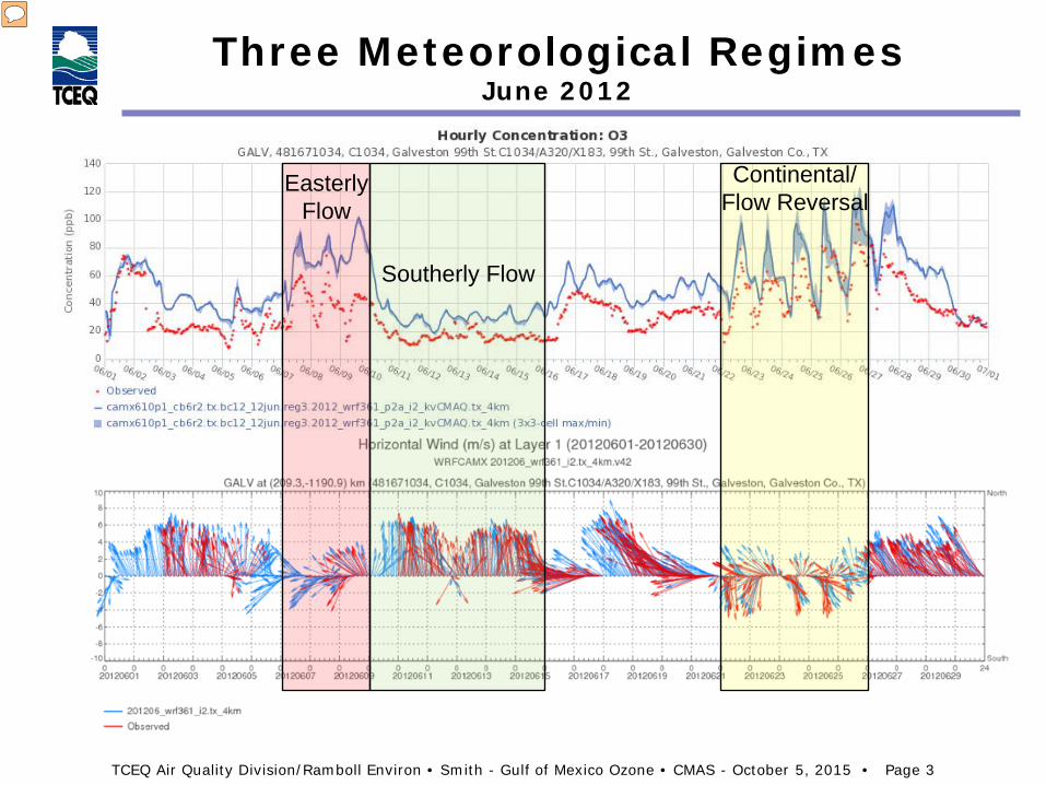
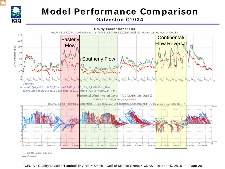
Three Meteorological Regimes June 2012
Easterly Flow
Southerly Flow
Continental/ Flow Reversal
Presenter
Presentation Notes
Examples of three distinct meteorological regimes are highlighted: Easterly flow – model shows some pretty serious over-prediction (25 to over 50 ppb) except for a couple of hours on June 8. Southerly flow – Clean air from Gulf of Mexico, model generally over-predicts by 10-20 ppb Continental Air with Flow Reversal – Model over-predicts but one-hour peaks are generally within the 3X3 grid cell array containing the monitor.
TCEQ Air Quality Division/Ramboll Environ • Smith - Gulf of Mexico Ozone • CMAS - October 5, 2015 • Page 4
Three Meteorological Regimes June 2012
Easterly Flow
Continental/ Flow Reversal
Southerly Flow
June 7-9, 2012 14:00 back trajectories, 50m agl at Galveston
June 10-15, 2012 14:00 back trajectories, 50m agl at Galveston
June 22-26, 2012 14:00 back trajectories, 50m agl at Galveston
Presenter
Presentation Notes
HySplit Back trajectories at 14:00, terminating at 50 m above Galveston monitor, associated with each highlighted regime. In the Easterly Flow regime air originating in southern Louisiana and farther east encounters the surf zone as it approaches Galveston. Southerly flow brings air from the mid to southern Gulf to Galveston, and Continental/Flow Reversal conditions combine continental background air with recirculated local emissions. Ozone contours/back trajectories were developed using TCEQ’s Geo-Referenced Interactive Model Results Evaluation and Analysis Program (GRIMREAPr) – See Doug Boyer’s poster & demonstration during Poster Session 2 Tuesday at 5:30 in the Model Evaluation and Analysis session.
TCEQ Air Quality Division/Ramboll Environ • Smith - Gulf of Mexico Ozone • CMAS - October 5, 2015 • Page 5
Halogen Chemistry in CAMx
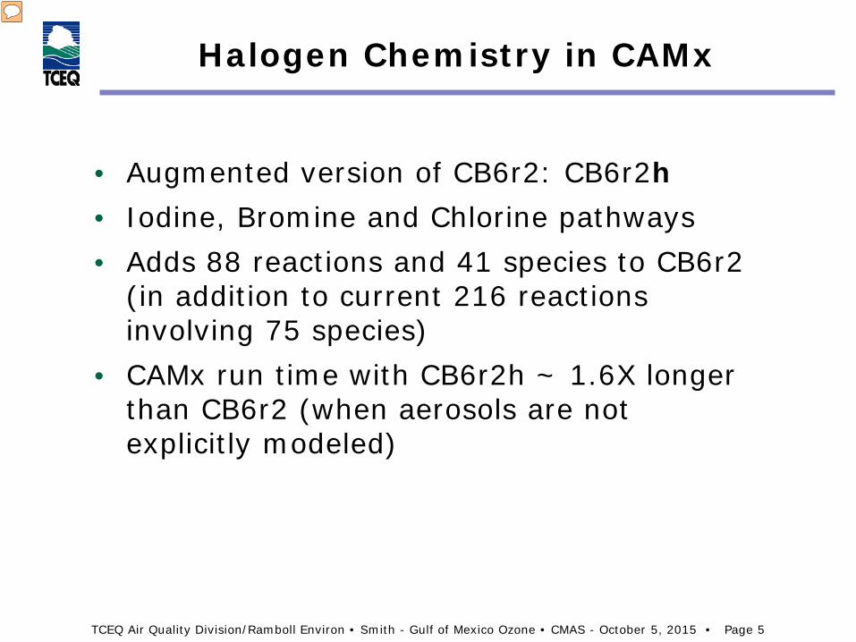
• Augmented version of CB6r2: CB6r2h • Iodine, Bromine and Chlorine pathways • Adds 88 reactions and 41 species to CB6r2
(in addition to current 216 reactions involving 75 species)
• CAMx run time with CB6r2h ~ 1.6X longer than CB6r2 (when aerosols are not explicitly modeled)
Presenter
Presentation Notes
CB6r2 – Carbon-Bond version 6 release 2 CB6r2h – Carbon-Bond version 6 release 2 with halogen chemistry
TCEQ Air Quality Division/Ramboll Environ • Smith - Gulf of Mexico Ozone • CMAS - October 5, 2015 • Page 6
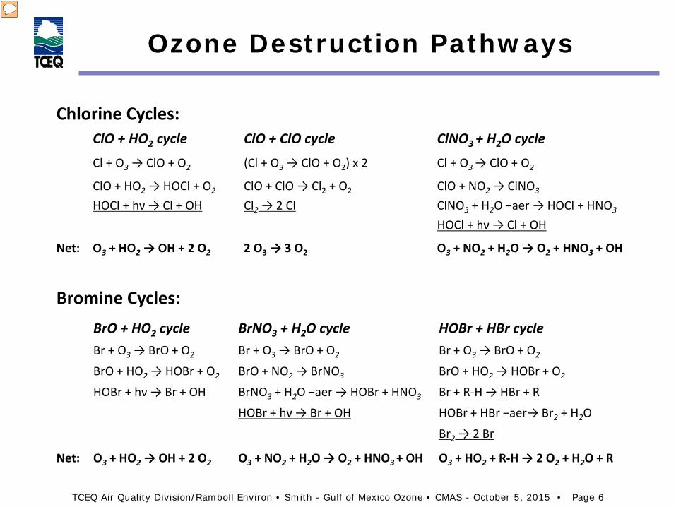
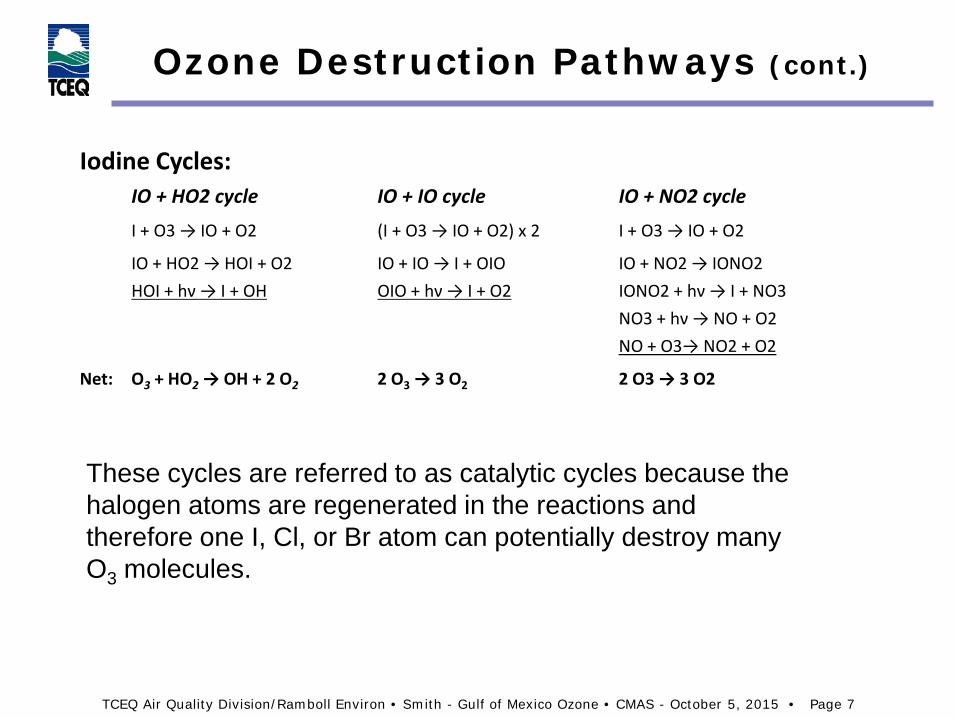
Chlorine, Iodine, and Bromine compounds all participate in reaction cycles which convert ozone into molecular oxygen, leaving the halogens available for additional reactions.
TCEQ Air Quality Division/Ramboll Environ • Smith - Gulf of Mexico Ozone • CMAS - October 5, 2015 • Page 7
I + O3 → IO + O2 (I + O3 → IO + O2) x 2 I + O3 → IO + O2
IO + HO2 → HOI + O2 IO + IO → I + OIO IO + NO2 → IONO2 HOI + hν → I + OH OIO + hν → I + O2 IONO2 + hν → I + NO3
NO3 + hν → NO + O2 NO + O3→ NO2 + O2
Net: O3 + HO2 → OH + 2 O2 2 O3 → 3 O2 2 O3 → 3 O2
These cycles are referred to as catalytic cycles because the halogen atoms are regenerated in the reactions and therefore one I, Cl, or Br atom can potentially destroy many O3 molecules.
TCEQ Air Quality Division/Ramboll Environ • Smith - Gulf of Mexico Ozone • CMAS - October 5, 2015 • Page 8
Halogen Emissions
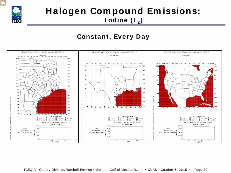
• Molecular iodine (I2, CB6h species I2) emissions from seawater are assigned a constant flux of 4X10⁸ molecules cm-2sec-1.
• Chlorine and bromine-content of sea salt aerosols (SSCL and SSBR, respectively) are assumed to be produced by oceanic turbulence, bubble breaking, and viscous shear and are modeled using the CAMx sea-salt preprocessor.
TCEQ Air Quality Division/Ramboll Environ • Smith - Gulf of Mexico Ozone • CMAS - October 5, 2015 • Page 9
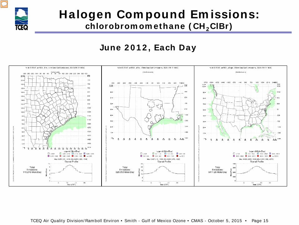
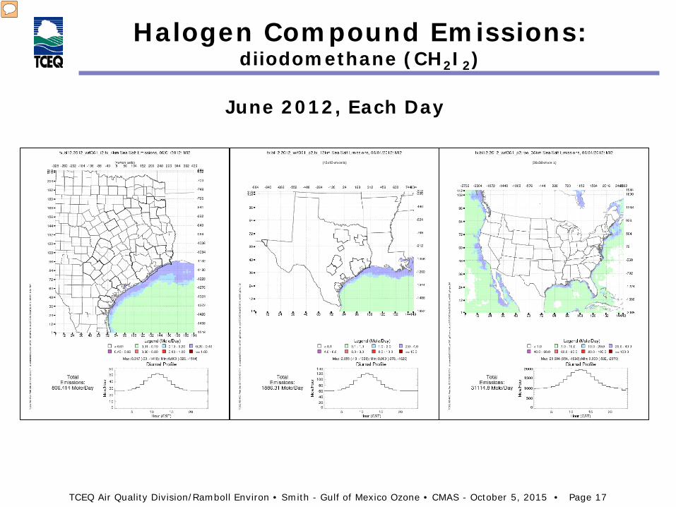
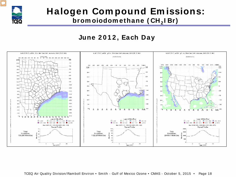
Halogen Emissions
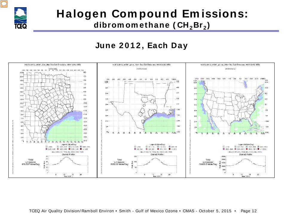
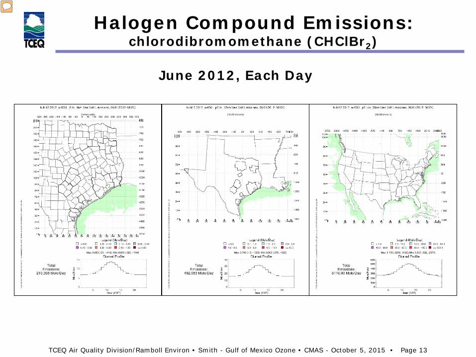
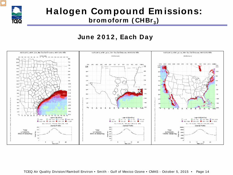
• Halomethanes are generated by organic sources and allocated spatially according to monthly average chlorophyll-a observations from the SeaWIFS satellite. These include: – Iodomethane (CH3I, CH3I) – Diiodomethane (CH2I2, MI2) – Chloroiodomethane (CH2ICl, MIC) – Bromoiodomethane (CH2IBr, MIB) – Chlorobromomethane (CH2BrCl, MBC) – Dibromomethane (CH2Br2, MB2) – Dichlorobromomethane (CHBrCl2,MBC2) – Chlorodibromomethane (CHBr2Cl, MB2C) – Bromoform (CHBr3, MB3)
Presenter
Presentation Notes
SeaWIFS – Sea-viewing Wide Field-of-view Sensor.
TCEQ Air Quality Division/Ramboll Environ • Smith - Gulf of Mexico Ozone • CMAS - October 5, 2015 • Page 10
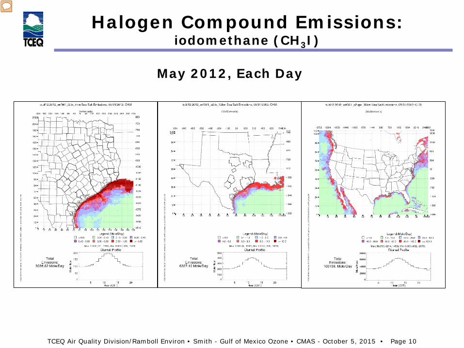
Halogen Compound Emissions: iodomethane (CH3I)
May 2012, Each Day
Presenter
Presentation Notes
Iodomethane is mostly emitted near shorelines where chlorophyll-a is found in the highest concentrations. Note emissions peak at noon local time.
TCEQ Air Quality Division/Ramboll Environ • Smith - Gulf of Mexico Ozone • CMAS - October 5, 2015 • Page 11
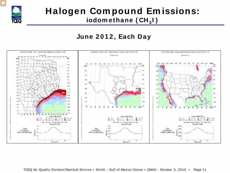
Halogen Compound Emissions: iodomethane (CH3I)
June 2012, Each Day
Presenter
Presentation Notes
June daily emissions of iodomethane shows some differences from May (due to differing monthly average chlorophyll-a measurements from SeaWIFS).
TCEQ Air Quality Division/Ramboll Environ • Smith - Gulf of Mexico Ozone • CMAS - October 5, 2015 • Page 12
Hidden slide: June daily emissions of chloroiodomethane
TCEQ Air Quality Division/Ramboll Environ • Smith - Gulf of Mexico Ozone • CMAS - October 5, 2015 • Page 20
Halogen Compound Emissions: Iodine (I2)
Constant, Every Day
Presenter
Presentation Notes
Iodine is assumed to be emitted continuously at a constant rate over all ocean waters.
TCEQ Air Quality Division/Ramboll Environ • Smith - Gulf of Mexico Ozone • CMAS - October 5, 2015 • Page 23
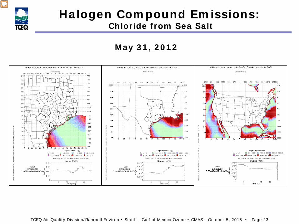
Halogen Compound Emissions: Chloride from Sea Salt
May 31, 2012
Presenter
Presentation Notes
Sea-salt Chloride May 31 2012. Wave action is driven by winds from the meteorological model. Emissions along the coastlines result from breaking waves in the surf zone. Note emissions vary dramatically from hour-to-hour and day-to-day.
TCEQ Air Quality Division/Ramboll Environ • Smith - Gulf of Mexico Ozone • CMAS - October 5, 2015 • Page 24
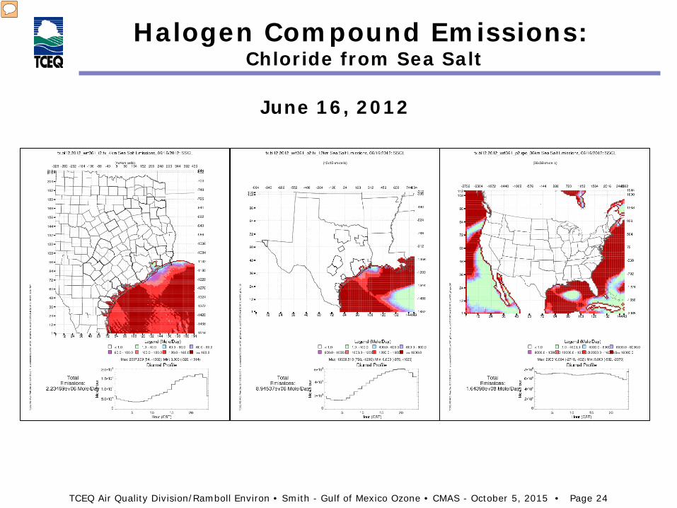
Halogen Compound Emissions: Chloride from Sea Salt
June 16, 2012
Presenter
Presentation Notes
Sea-salt Chloride June 16 2012.
TCEQ Air Quality Division/Ramboll Environ • Smith - Gulf of Mexico Ozone • CMAS - October 5, 2015 • Page 25
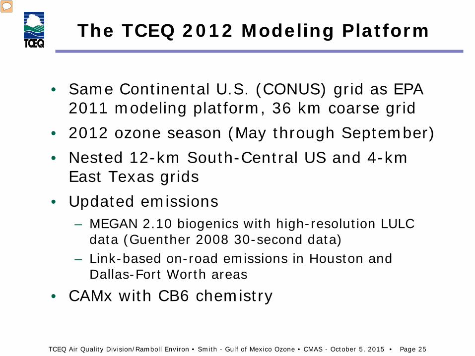
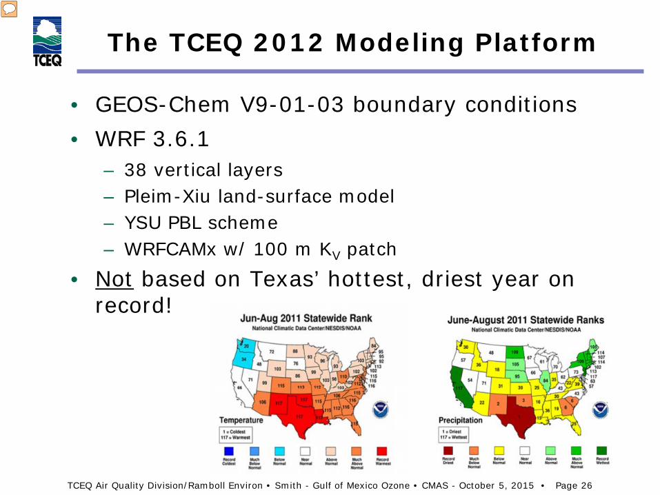
The TCEQ 2012 Modeling Platform
• Same Continental U.S. (CONUS) grid as EPA 2011 modeling platform, 36 km coarse grid
• 2012 ozone season (May through September) • Nested 12-km South-Central US and 4-km
East Texas grids • Updated emissions
– MEGAN 2.10 biogenics with high-resolution LULC data (Guenther 2008 30-second data)
– Link-based on-road emissions in Houston and Dallas-Fort Worth areas
• CAMx with CB6 chemistry
Presenter
Presentation Notes
MEGAN – Model of Emissions from Gas and Nature LULC – Land Use/Land Cover CAMx – Comprehensive Air quality Model with Extensions
TCEQ Air Quality Division/Ramboll Environ • Smith - Gulf of Mexico Ozone • CMAS - October 5, 2015 • Page 26
– 38 vertical layers – Pleim-Xiu land-surface model – YSU PBL scheme – WRFCAMx w/ 100 m KV patch
• Not based on Texas’ hottest, driest year on record!
Presenter
Presentation Notes
The historic 2011 drought far surpassed any of the last 120 years as the hottest and driest year on record. It would be ill-advised to use a 2011 as a base year for State Implementation Planning since an attainment demonstration based on a wildly abnormal year may not be appropriate for years with more normal meteorology. GEOS-Chem – Goddard Earth Observing System model with Chemistry YSU PBL scheme – Yonsei University Planetary Boundary Layer scheme WRFCAMx – Weather Research and Forecasting model (WRF) to CAMx interface program Kv – Vertical diffusivity
TCEQ Air Quality Division/Ramboll Environ • Smith - Gulf of Mexico Ozone • CMAS - October 5, 2015 • Page 27
The TCEQ 2012 Modeling Platform
Texas Ozone Modeling Domains
Presenter
Presentation Notes
Texas 2012 Modeling Platform outer (36 kilometer X 36 kilometer, or just 36 km) grid covers continental US including much of southern Canada and northern Mexico plus Cuba and the Bahamas. The 12 km grid covers all or most of of the surrounding states of most of New Mexico, Oklahoma, Louisiana, Arkansas, and Mississippi, along with parts of other south-central states and a large portion of northern Mexico. The 4 km grid covers eastern Texas except for far South Texas and includes parts of Oklahoma, Louisiana, Arkansas, and Mexico. 38 vertical layers grow progressively thicker as they increase in altitude to approximately 15000 meters.
TCEQ Air Quality Division/Ramboll Environ • Smith - Gulf of Mexico Ozone • CMAS - October 5, 2015 • Page 28
Model Performance Comparison Galveston C1034
Easterly Flow
Southerly Flow
Continental/ Flow Reversal
Presenter
Presentation Notes
Time series shows model performance improves by reducing modeled ozone concentrations by a few ppb under southerly and easterly flow. In the continental/flow reversal case only marginal improvement is seen.
TCEQ Air Quality Division/Ramboll Environ • Smith - Gulf of Mexico Ozone • CMAS - October 5, 2015 • Page 29
Model Performance Comparison Eastern Texas (4 km grid)
Area Number Monitors
Dallas-Fort Worth (DFW) 17
Houston-Galveston- Brazoria (HGB) 46
Beaumont-Port Arthur (BPA) 8
Northeast Texas (NETX) 3
Central Texas (CNTX) 17
Corpus Christi-Victoria (CCV) 10
Other areas 7
Eastern Texas Total (4 km grid) 109
BPA
DFW
CNTX
NETX
HGB CCV
Presenter
Presentation Notes
Six regions of Texas are selected for sub-regional model performance evaluation.
TCEQ Air Quality Division/Ramboll Environ • Smith - Gulf of Mexico Ozone • CMAS - October 5, 2015 • Page 30
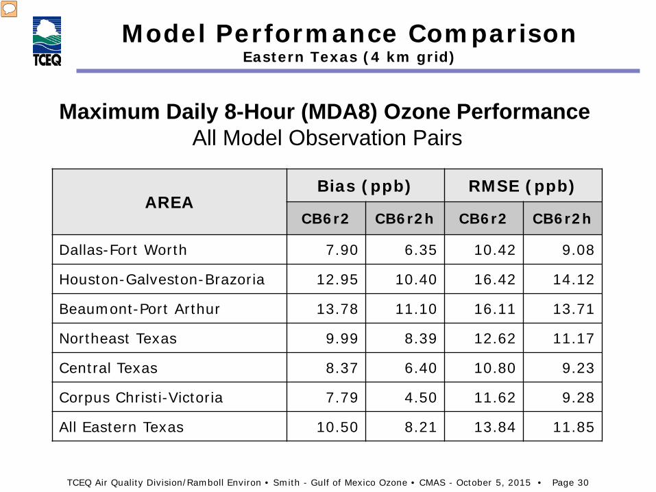
Model Performance Comparison Eastern Texas (4 km grid)
Maximum Daily 8-Hour (MDA8) Ozone Performance All Model Observation Pairs
Presenter
Presentation Notes
Chart shows significant positive bias in 30-day average MDA8 ozone concentrations. Using halogen chemistry reduces bias in every area between 1.5 to 3 ppb, with largest reductions near the coast. Root Mean Squared Error (RMSE) is reduced by up to 2 ppb.
TCEQ Air Quality Division/Ramboll Environ • Smith - Gulf of Mexico Ozone • CMAS - October 5, 2015 • Page 31
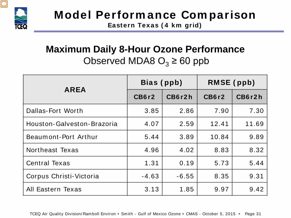
Model Performance Comparison Eastern Texas (4 km grid)
For MDA8 ozone ≥ 60 ppb, model bias and RMSE are considerably lower to begin with but still are positive except for Corpus Christi-Victoria. Model bias and RMSE still show notable improvements except for CCV which shows model performance worsening. May be some missing emission sources in Corpus Christi area. Bottom line is the model is doing a fairly good job predicting the higher MDA8 ozone concentrations, especially using halogen chemistry. Significant bias for lower concentrations, while reduced substantially though halogen chemistry, is still of concern.
TCEQ Air Quality Division/Ramboll Environ • Smith - Gulf of Mexico Ozone • CMAS - October 5, 2015 • Page 32
Marine Boundary Conditions
• Boundary conditions for regional modeling applications are typically extracted from global models such as GEOS-Chem and MOZART.
• Comparison of marine boundary conditions with near-shore monitors indicates that they over-predict ozone over ocean waters.
• Halogen chemistry is being included in newer versions of the global models.
Presenter
Presentation Notes
MOZART – Model of Ozone and Related Tracers
TCEQ Air Quality Division/Ramboll Environ • Smith - Gulf of Mexico Ozone • CMAS - October 5, 2015 • Page 33
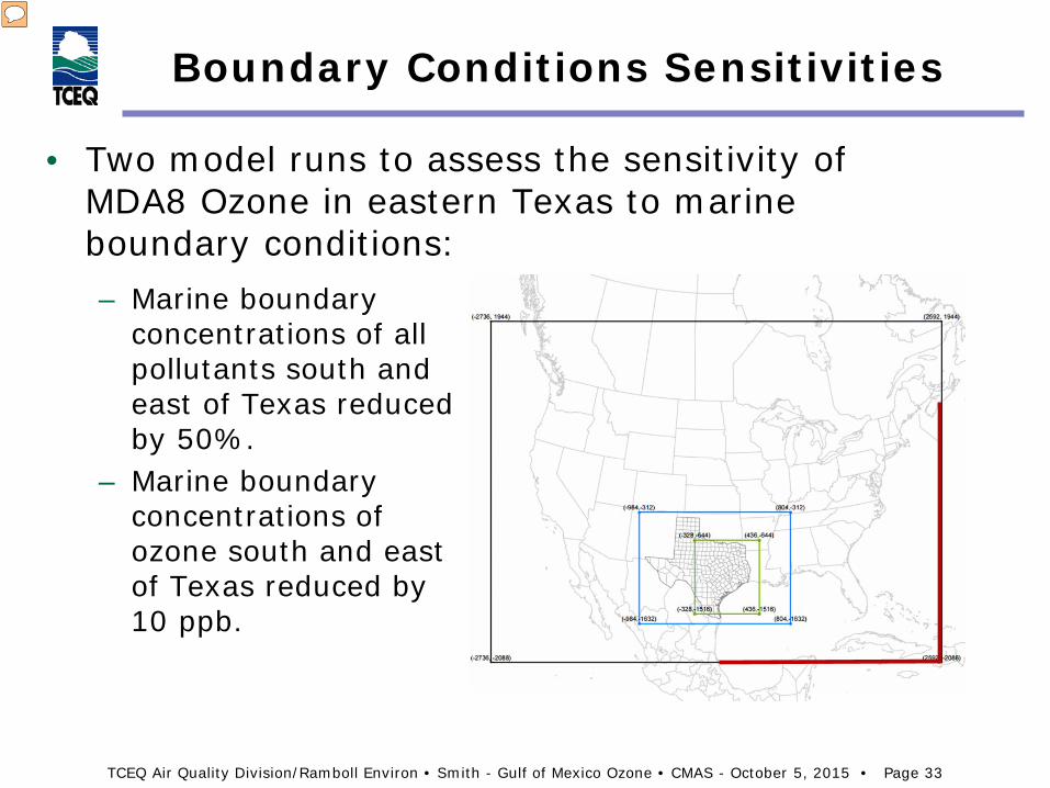
Boundary Conditions Sensitivities
• Two model runs to assess the sensitivity of MDA8 Ozone in eastern Texas to marine boundary conditions: – Marine boundary
concentrations of all pollutants south and east of Texas reduced by 50%.
– Marine boundary concentrations of ozone south and east of Texas reduced by 10 ppb.
Presenter
Presentation Notes
Red line denotes the approximate sections of the domain boundaries where emissions sensitivities were applied.
TCEQ Air Quality Division/Ramboll Environ • Smith - Gulf of Mexico Ozone • CMAS - October 5, 2015 • Page 34
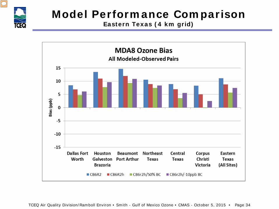
Model Performance Comparison Eastern Texas (4 km grid)
Presenter
Presentation Notes
Chart shows that bias for all model-observation pairs is reduced in every area and across the 4-km domain through using halogen chemistry. It is further reduced by several ppb using the (probably unrealistic) 50% reduction to south and east oceanic boundary conditions. Bias reductions using the 10 ppb across-the-board ozone cuts are more modest but still notable.
TCEQ Air Quality Division/Ramboll Environ • Smith - Gulf of Mexico Ozone • CMAS - October 5, 2015 • Page 35
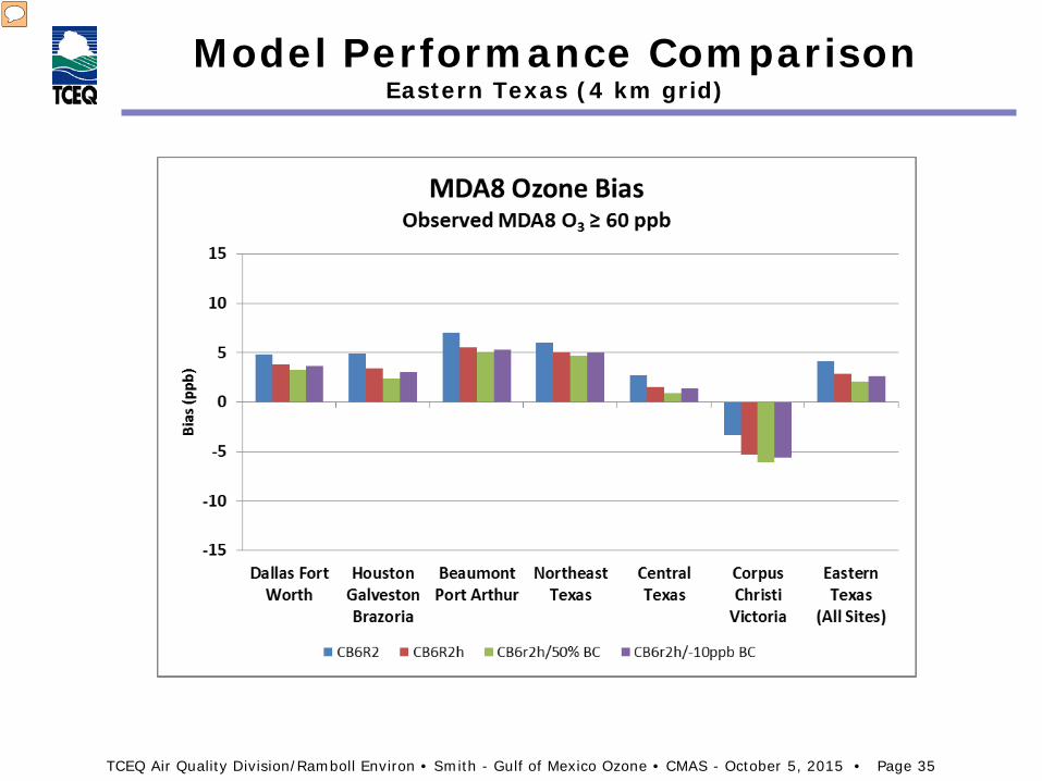
Model Performance Comparison Eastern Texas (4 km grid)
Presenter
Presentation Notes
Chart shows that bias for model-observation pairs with observed MDA8 ≥ 60 ppb concentrations is reduced in every area and across the 4-km domain through using halogen chemistry, but less than is seen for all pairs. Further bias reductions from the boundary condition sensitivity runs are fairly modest.
TCEQ Air Quality Division/Ramboll Environ • Smith - Gulf of Mexico Ozone • CMAS - October 5, 2015 • Page 36
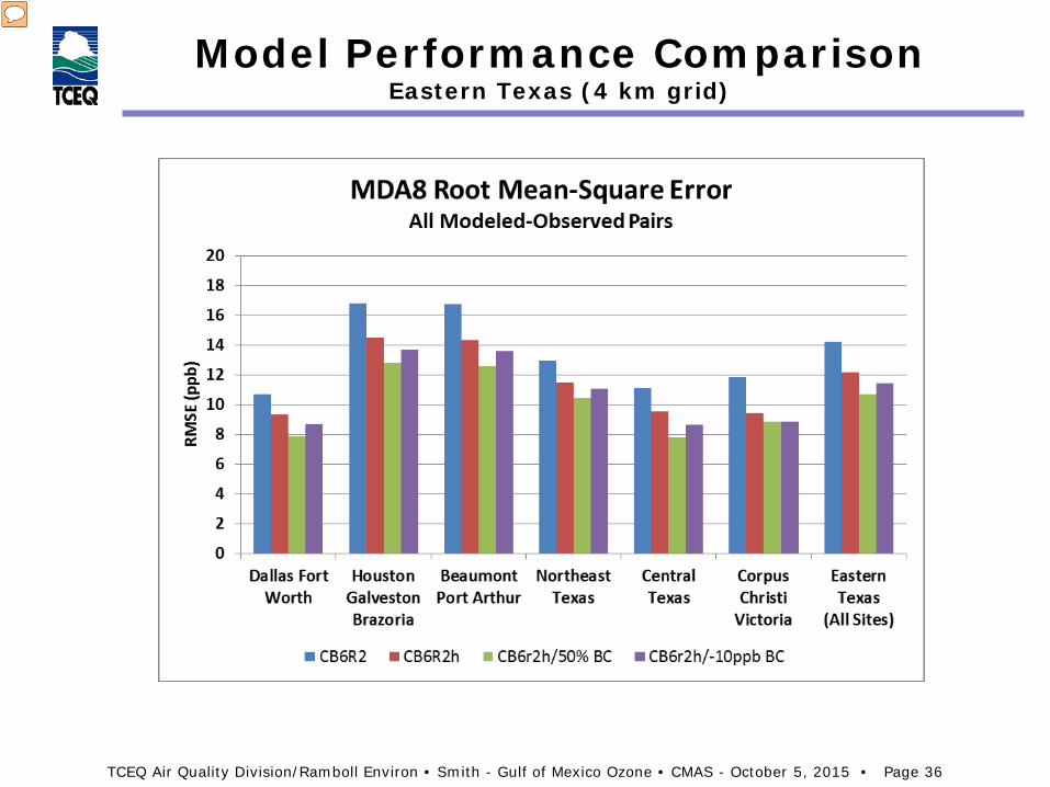
Model Performance Comparison Eastern Texas (4 km grid)
Presenter
Presentation Notes
Chart shows that RMSE for all model-observation pairs is reduced in every area and across the 4-km domain through using halogen chemistry. It is further reduced by several ppb using the (probably unrealistic) 50% reduction to south and east oceanic boundary conditions. RMSE reductions using the 10 ppb across-the-board ozone cuts are more modest but still notable.
TCEQ Air Quality Division/Ramboll Environ • Smith - Gulf of Mexico Ozone • CMAS - October 5, 2015 • Page 37
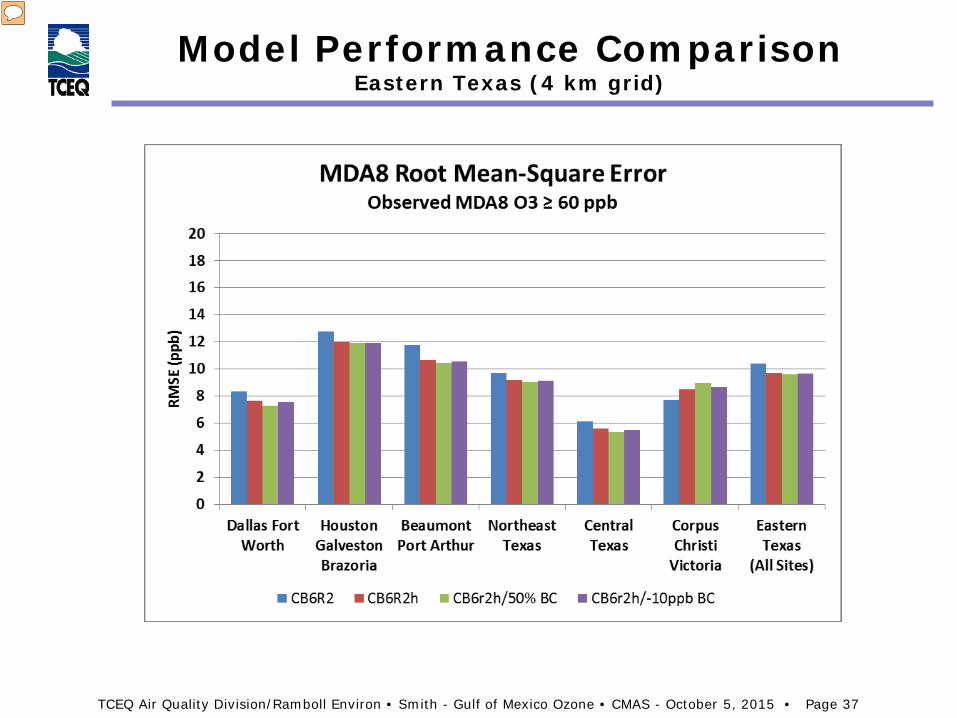
Model Performance Comparison Eastern Texas (4 km grid)
Presenter
Presentation Notes
Chart shows that RMSE for model-observation pairs with observed MDA8 ≥ 60 ppb concentrations is reduced in every area (except Corpus Christi) and across the 4-km domain through using halogen chemistry, but less than is seen for all pairs. Further RMSE reductions from the boundary condition sensitivity runs are fairly modest. Interestingly, the reductions in areas away from the Dallas-Fort Worth area shows greater response to the boundary condition reductions than do Houston-Galveston or Beaumont-Port Arthur. This is likely due to influence from the eastern boundary condition reductions on the DFW area.
TCEQ Air Quality Division/Ramboll Environ • Smith - Gulf of Mexico Ozone • CMAS - October 5, 2015 • Page 38
Conclusions
• Models over-predict ozone concentrations transported onshore from the Gulf of Mexico.
• Model performance can be significantly improved through use of halogen chemistry and through reduced marine boundary conditions.
• Smaller but still significant improvements are seen for MDA8 concentrations ≥ 60 ppb.
• Halogen chemistry increases CAMx execution time by about 60% when explicit aerosols are not being modeled.
TCEQ Air Quality Division/Ramboll Environ • Smith - Gulf of Mexico Ozone • CMAS - October 5, 2015 • Page 39
Future Needs
• Faster halogen chemistry code to reduce long execution times
• Monitoring of halogen products at Galveston (summer, 2016)
• New boundary conditions from a global model with native halogen chemistry (“almost there” in GEOS-Chem)
• Investigation of iodine feedback loop – ozone deposition on ocean waters releases I2, which in turn reacts with ozone
TCEQ Air Quality Division/Ramboll Environ • Smith - Gulf of Mexico Ozone • CMAS - October 5, 2015 • Page 40
Resources
• The TCEQ 2012 modeling platform can be accessed at: https://www.tceq.texas.gov/airquality/airmod/data/tx2012 (currently June is online but other months should be available soon).
• Ozone background references: – Estes, M., D. Johnston, F. Mercado and Smith, J (2014) Regional
background ozone in the eastern half of Texas, Presented at CMAS 2014 http://www.cmascenter.org/conference/2014/agenda.cfm
– Smith, J., F. Mercado and M. Estes (2013). Characterization of Gulf of Mexico Background Ozone Concentrations, Presented at CMAS 2013 http://www.cmascenter.org/conference/2013/agenda.cfm
• Marine halogen chemistry references: – Yarwood, G., J. Jung, U. Nopmongcol and C. Emery (2012) Improving
CAMx Performance in Simulating Ozone Transport from the Gulf of Mexico, Final Report for Work Order No. 582-11-10365-FY12-05
– Yarwood, G., T. Sakulyanontvittaya, U. Nopmongcol and B. Koo (2015). Ozone Depletion by Bromine and Iodine over the Gulf of Mexico, Final Report for Work Order No. 582-11-10365-FY14-12 https://www.tceq.texas.gov/airquality/airmod/project/pj_report_pm.html
– Monks, et al., 2015, Tropospheric ozone and its precursors from the urban to the global scale from air quality to short-lived climate forcer, Atmos. Chem. Phys., 15, 8889–8973, 2015