Addressing Non-CO 2 Gases & Sinks in GHG Scenarios: Experience from Energy Modeling Forum 21 Francisco C. de la Chesnaye US Environmental Protection Agency John P. Weyant Stanford University NIES - EMF Workshop on GHG Stabilization Scenarios, Tsukuba, 22-23 January 2004
Transcript
Addressing Non-CO2 Gases & Sinks in GHG Scenarios: Experience from Energy Modeling
Forum 21
Francisco C. de la ChesnayeUS Environmental Protection Agency
John P. WeyantStanford University
NIES - EMF Workshop on GHG Stabilization Scenarios, Tsukuba, 22-23 January 2004
Outline
º Introduction to the EMF 21 Studyº Data Development on Non-CO2 GHG and Sinksº Results part A: Non-CO2 GHGs º Areas for further work
º Results part B: Recent EMF 21 Scenario Runs
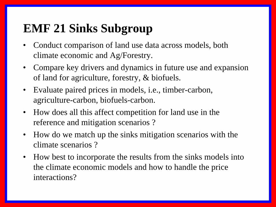
EMF 21 Working Group Objectives
1) Conduct a new comprehensive, multi-gas policy assessment to improve the understanding of the affects of including non-CO2 GHGs (NCGGs) and sinks (terrestrial sequestration) into short- and long-term mitigation policies. Answer the question: How important are NCGGs & Sinks in climate policies?.
2) Advance the state-of-the-art in integrated assessment / economic modeling
3) Strengthen collaboration between NCGG and Sinks experts and modeling teams
4) Publish results in a special issue of the Energy Journal
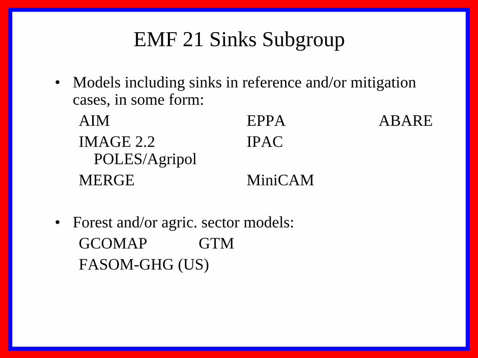
Economy, Technology, & Integrated Assessment Models (18)Asia / Australia ABARE (Guy Jakeman & Brian Fisher) with GTEMEnergy Research Institute China (Jiang Kejun) with IPACIAE Japan (Atsushi Kurosawa) with GRAPEIndian Institute of Management (P. Shukla) with SGM-India National Institute for Environmental Studies, Japan (Junichi Fujino) with AIM
EuropeCEA - IDEI (Marc Vielle) with GEMINI-E3 CICERO - University of Oslo (H.A. Aaheim) with COMBATCntr for European Econ Research-(C. Boehringer & A. Loschel) with EU PACECopenhagen Economics (Jesper Jensen) with the EDGE Model Hamburg Univ. (Richard Tol) with FUNDIIASA (Shilpa Rao) with MESSAGEOldenburg University, Germany (Claudia Kemfert) with WIAGEMRIVM (Detlef van Vuuren, Tom Kram, & Bas Eickhout) with IMAGE UPMF (Patrick Criqui) & CIRAD (Daniel Deybe) with POLES/AGRIPOL
USArgonne Nat Lab (Don Hanson) & EPA (Skip Laitner) with AMIGAEPRI (Rich Richels) & Stanford Univ (Alan Manne) with MERGEMIT (John Reilly) with EPPAPNNL-JGCRI (Jae Edmonds, Hugh Pitcher, & Steve Smith) with SGM & MiniCAM
Non-CO2 GHG ExpertsDina Kruger and Francisco de la Chesnaye, USEPAPaul Freund and John Gale, IEA Greenhouse Gas R&D Programme
Methane & N2OAnn Gardiner, Judith Bates, AEA TechnologyCasey Delhotal, Dina Kruger, Elizabeth Scheehle, USEPAChris Hendriks, Niklas Hoehne, EcofysFluorinated (HGWP) Gases Jochen Harnish, Ecofys, GermanyDeborah Ottinger and Dave Godwin, USEPA
Sinks (Terrestrial Sequestration) Bruce McCarl, Texas A&MKen Andrasko, USEPA & Jayant Sathaye, LBNLRoger Sedjo, RFF & Brent Sohngen, Ohio State Univ Ron Sands, PNNL-JGCRI
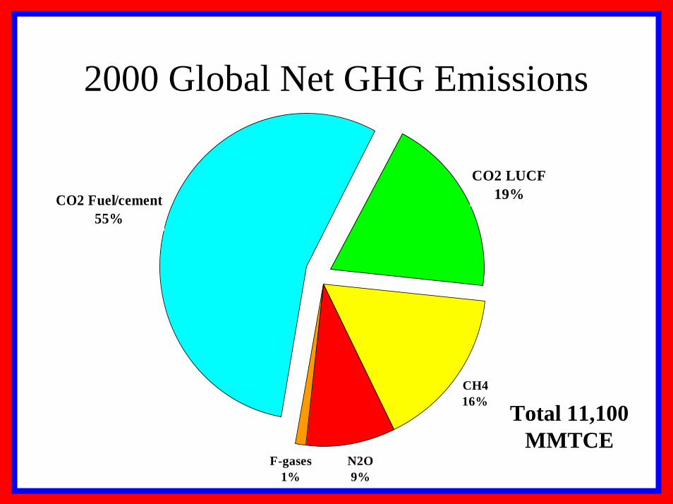
CH416%
N2O9%
F-gases1%
CO2 LUCF19%
2000 Global Net GHG Emissions
CO2 Fuel/cement55%
Total 11,100 MMTCE
Non-CO2 GHG & sequestration data requirements
• Global, consistent non-CO2 GHG emission baselines for 2000 and projections 2020 by region. And key emissions drivers.
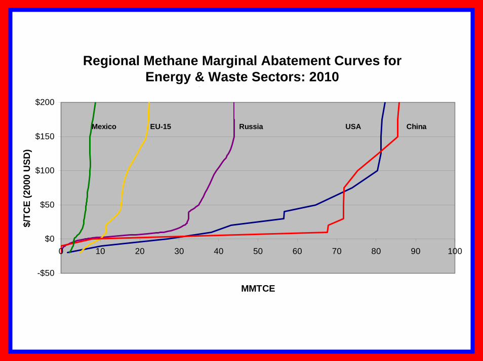
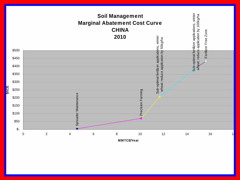
• Comparable marginal abatement curves – by region, by gas, and by sector– sensitivities to energy, material prices – in MMTCE w/ 100-yr GWP & gas specific units– Various discount and tax rates
• Assessment of how marginal abatement curves vary over time, from 2010 to 2100 by decade.
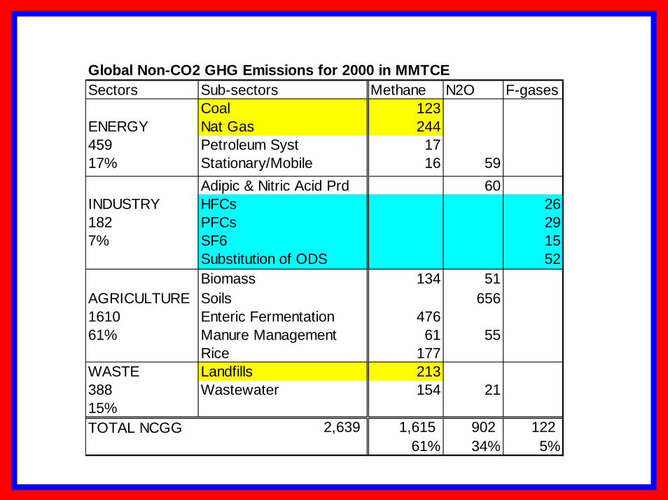
Global Non-CO2 GHG Emissions for 2000 in MMTCESectors Sub-sectors Methane N2O F-gases
Coal 123ENERGY Nat Gas 244459 Petroleum Syst 1717% Stationary/Mobile
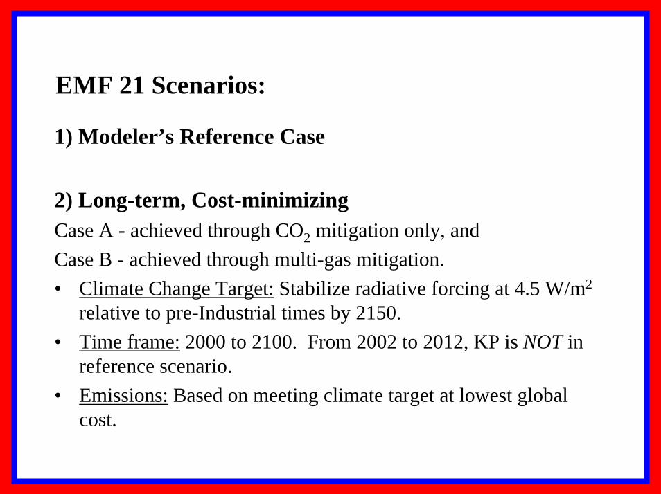
2) Long-term, Cost-minimizingCase A - achieved through CO2 mitigation only, and Case B - achieved through multi-gas mitigation.• Climate Change Target: Stabilize radiative forcing at 4.5 W/m2
relative to pre-Industrial times by 2150. • Time frame: 2000 to 2100. From 2002 to 2012, KP is NOT in
reference scenario.• Emissions: Based on meeting climate target at lowest global
cost.
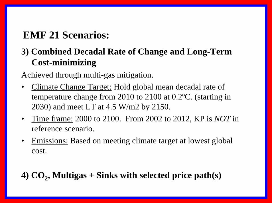
EMF 21 Scenarios:3) Combined Decadal Rate of Change and Long-Term
Cost-minimizingAchieved through multi-gas mitigation. • Climate Change Target: Hold global mean decadal rate of
temperature change from 2010 to 2100 at 0.2ºC. (starting in 2030) and meet LT at 4.5 W/m2 by 2150.
• Time frame: 2000 to 2100. From 2002 to 2012, KP is NOT in reference scenario.
• Emissions: Based on meeting climate target at lowest global cost.
4) CO2, Multigas + Sinks with selected price path(s)
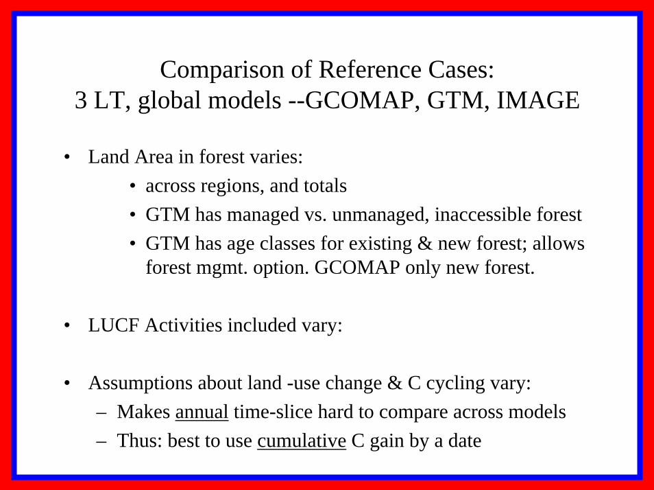
Comparison of Reference Cases:3 LT, global models --GCOMAP, GTM, IMAGE
• Land Area in forest varies: • across regions, and totals• GTM has managed vs. unmanaged, inaccessible forest• GTM has age classes for existing & new forest; allows
forest mgmt. option. GCOMAP only new forest.
• LUCF Activities included vary:
• Assumptions about land -use change & C cycling vary:– Makes annual time-slice hard to compare across models– Thus: best to use cumulative C gain by a date
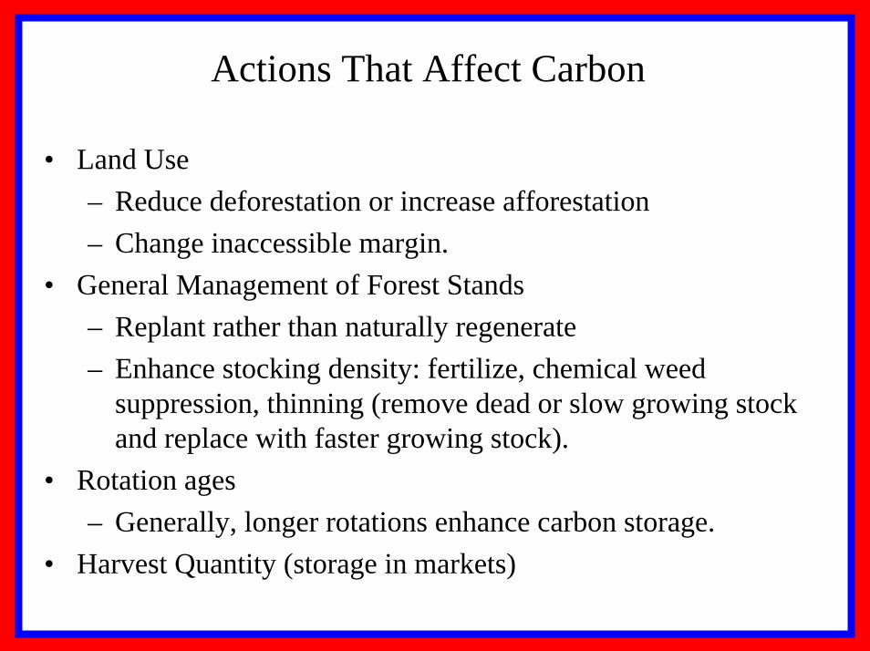
Actions That Affect Carbon
• Land Use – Reduce deforestation or increase afforestation– Change inaccessible margin.
• General Management of Forest Stands – Replant rather than naturally regenerate– Enhance stocking density: fertilize, chemical weed
suppression, thinning (remove dead or slow growing stock and replace with faster growing stock).
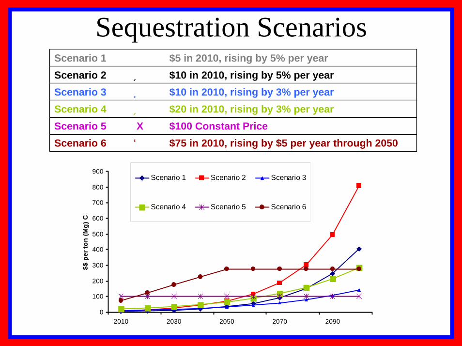
$75 in 2010, rising by $5 per year through 2050●Scenario 6$100 Constant PriceXScenario 5$20 in 2010, rising by 3% per year■Scenario 4$10 in 2010, rising by 3% per year▲Scenario 3$10 in 2010, rising by 5% per year■Scenario 2$5 in 2010, rising by 5% per year♦Scenario 1
0
100
200
300
400
500
600
700
800
900
2010 2030 2050 2070 2090
$$ p
er to
n (M
g) C
Scenario 1 Scenario 2 Scenario 3
Scenario 4 Scenario 5 Scenario 6
ScaleResults for 2100
Price Cum. C Land Temp. Trop.$$ per ton Pg Million ha % %
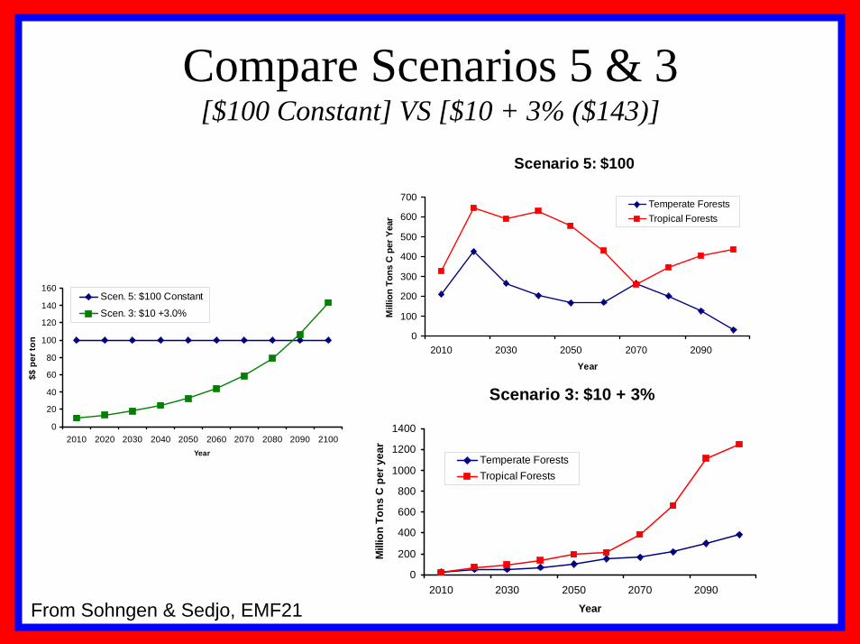
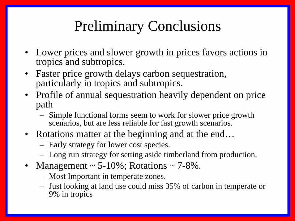
• Lower prices and slower growth in prices favors actions in tropics and subtropics.
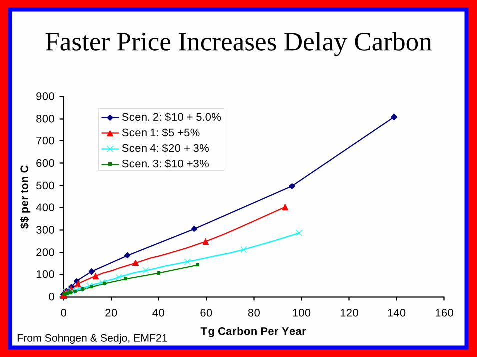
• Faster price growth delays carbon sequestration, particularly in tropics and subtropics.
• Profile of annual sequestration heavily dependent on price path– Simple functional forms seem to work for slower price growth
scenarios, but are less reliable for fast growth scenarios.• Rotations matter at the beginning and at the end…
– Early strategy for lower cost species.– Long run strategy for setting aside timberland from production.
• Management ~ 5-10%; Rotations ~ 7-8%.– Most Important in temperate zones.– Just looking at land use could miss 35% of carbon in temperate or
9% in tropics
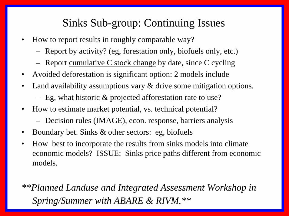
Sinks Sub-group: Continuing Issues• How to report results in roughly comparable way?
– Report by activity? (eg, forestation only, biofuels only, etc.)– Report cumulative C stock change by date, since C cycling
• Avoided deforestation is significant option: 2 models include• Land availability assumptions vary & drive some mitigation options.
– Eg, what historic & projected afforestation rate to use?• How to estimate market potential, vs. technical potential?
– Decision rules (IMAGE), econ. response, barriers analysis• Boundary bet. Sinks & other sectors: eg, biofuels• How best to incorporate the results from sinks models into climate
economic models? ISSUE: Sinks price paths different from economic models.
**Planned Landuse and Integrated Assessment Workshop in Spring/Summer with ABARE & RIVM.**
Carbon Storage in Forests
700
750
800
850
900
950
2000 2020 2040 2060 2080 2100
Year
Bill
ion
Met
ric T
on
Baseline$5 scenario$20 scenario
Carbon Price = $244 per ton
Carbon Price = $61 per ton
Carbon Price = $0 per ton
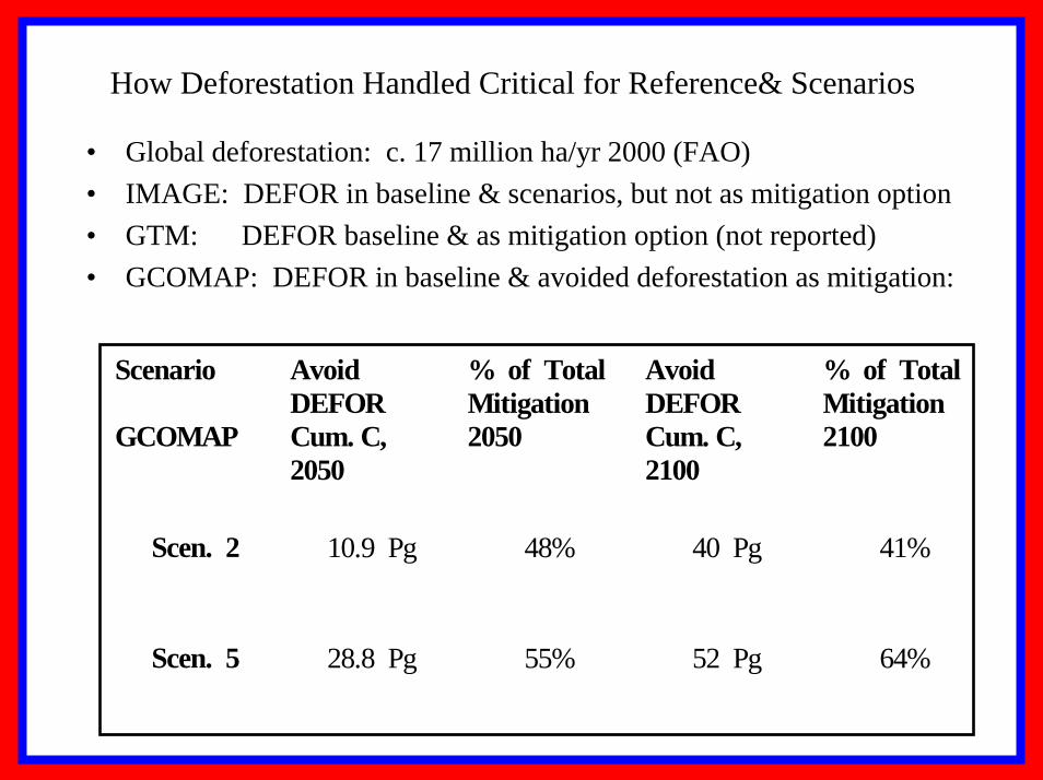
How Deforestation Handled Critical for Reference& Scenarios
• Global deforestation: c. 17 million ha/yr 2000 (FAO)• IMAGE: DEFOR in baseline & scenarios, but not as mitigation option• GTM: DEFOR baseline & as mitigation option (not reported)• GCOMAP: DEFOR in baseline & avoided deforestation as mitigation: