Page 1
ADDRESSING VARIABILITY OF FIBER PREFORM PERMEABILITY
IN PROCESS DESIGN FOR LIQUID COMPOSITE MOLDING
by
Hatice Sinem Sas
A dissertation submitted to the Faculty of the University of Delaware in partial
fulfillment of the requirements for the degree of Doctor of Philosophy in Mechanical
Engineering
Summer 2015
© 2015 Hatice Sinem Sas
All Rights Reserved
Page 2
All rights reserved
INFORMATION TO ALL USERSThe quality of this reproduction is dependent upon the quality of the copy submitted.
In the unlikely event that the author did not send a complete manuscriptand there are missing pages, these will be noted. Also, if material had to be removed,
a note will indicate the deletion.
All rights reserved.
This work is protected against unauthorized copying under Title 17, United States CodeMicroform Edition © ProQuest LLC.
ProQuest LLC.789 East Eisenhower Parkway
P.O. Box 1346Ann Arbor, MI 48106 - 1346
ProQuest 3730200
Published by ProQuest LLC (2015). Copyright of the Dissertation is held by the Author.
ProQuest Number: 3730200
Page 3
ADDRESSING VARIABILITY OF FIBER PREFORM PERMEABILITY
IN PROCESS DESIGN FOR LIQUID COMPOSITE MOLDING
by
Hatice Sinem Sas
Approved: __________________________________________________________
Suresh G. Advani, Ph.D.
Chair of the Department of Mechanical Engineering
Approved: __________________________________________________________
Babatunde A. Ogunnaike, Ph.D.
Dean of the College of Engineering
Approved: __________________________________________________________
James G. Richards, Ph.D.
Vice Provost for Graduate and Professional Education
Page 4
I certify that I have read this dissertation and that in my opinion it meets
the academic and professional standard required by the University as a
dissertation for the degree of Doctor of Philosophy.
Signed: __________________________________________________________
Suresh G. Advani, Ph.D.
Professor in charge of dissertation
I certify that I have read this dissertation and that in my opinion it meets
the academic and professional standard required by the University as a
dissertation for the degree of Doctor of Philosophy.
Signed: __________________________________________________________
James L. Glancey, Ph.D, P.E.
Member of dissertation committee
I certify that I have read this dissertation and that in my opinion it meets
the academic and professional standard required by the University as a
dissertation for the degree of Doctor of Philosophy.
Signed: __________________________________________________________
Rakesh, Ph.D.
Member of dissertation committee
I certify that I have read this dissertation and that in my opinion it meets
the academic and professional standard required by the University as a
dissertation for the degree of Doctor of Philosophy.
Signed: __________________________________________________________
Pavel Simacek, Ph.D.
Member of dissertation committee
Page 5
iv
ACKNOWLEDGMENTS
I would like to express my sincere gratitude to my advisor, Prof. Suresh G.
Advani, for the continuous support, patience, and enthusiasm he has provided during
my Ph.D. journey. I feel extremely lucky to have been mentored by someone with
deep knowledge, solid experience and infinite motivation to learn, teach, investigate
and invent.
I would like to thank Dr. Pavel Simacek for his support and advice on process
modeling and numerical simulation, and agreeing to serve on my dissertation
committee.
I acknowledge and give thanks to my other two committee members, Prof.
James Glancey and Prof. Rakesh for generously devoting time to judge my work and
providing insightful comments.
I would also like to thank many colleagues who worked with me during my
time in Delaware. I had the privilege to work with Jeffrey Lugo and Eric Wurtzel, and
with Louis Agostino and Minyoung Yun. I was lucky to have Richard Readdy for his
help in countless lab and LabVIEW problems. I want to express my gratitude to Dr.
Volkan Eskizeybek for his valuable advice. Also, I am grateful for the support and
friendship of the rest of my research group: Dr. John Gangloff, Thomas Cender, Jiayin
Wang, Dr. Hang Yu, Hong Yu and Michael Yeager.
I would also like to thank all of my office mates in Spencer007, CCM118 and
CCM123 (The Pit). Thank you all for the good times and friendship that we share.
Page 6
v
I would also like to thank the administrative staff of the Mechanical
Engineering Department: Lisa Katzmire, Ann Connor and Letitia Toto and Center for
Composite Materials: Corinne Hamed, Robin Mack, Penny O’Donnell, Therese
Stratton and Megan Hancock. I am thankful for your hard work and smiles.
I would also like to thank all of my dear friends for making the bad times good,
and the good times even better. I want to give special thanks to Sumeyra Yildirim,
Deniz Ozdiktas, and Sezin Zengin for their friendship and support. Also, I am lucky to
have Ozan Erol and Sinan Boztepe both as friends and colleagues in CCM. I am
feeling lucky to have the chance to meet my dearest friend Sevil Buzcu. She made my
Ph.D journey colorful and cheerful. We shared our moments for five years and we will
continue to do so. I am also grateful to my friend Furkan Cayci for the perspectives he
brought into my life. I am also thankful to him for his contribution to my research
using his software skills that made this dissertation complete. I also want to thank Filiz
Yesilkoy for not only being a best friend, but also being an inspiration and motivation
for my studies and my life. She says, “Life is all about asking the right question.” and
I know we will keep looking for questions together.
Lastly, I would like to thank my family. Mom, Dad and my sister Senem,
thanks for your unconditional love and endless support. I am deeply thankful to all of
my family members for their support.
I want to dedicate this dissertation to my grandmother who foresees my future
in academia. We built this dream with her. I know she is watching me from heaven
and will continue to send her blessings.
Rumi says, “Be grateful for whoever comes, because each has been sent as a
guide from beyond.” and I am grateful to everyone who touched my life.
Page 7
vi
TABLE OF CONTENTS
LIST OF TABLES ........................................................................................................ ix
LIST OF FIGURES ........................................................................................................ x ABSTRACT ................................................................................................................. xv
Chapter
1 INTRODUCTION .............................................................................................. 1
1.1 Liquid Composite Molding ....................................................................... 1
1.1.1 Materials used in LCM .................................................................. 2
1.1.1.1 Reinforcements ............................................................... 2 1.1.1.2 Matrices .......................................................................... 4
1.1.2 The LCM Family of Processes ...................................................... 5
1.1.2.1 The Resin Transfer Molding .......................................... 5 1.1.2.2 Vacuum Assisted Resin Transfer Molding ..................... 8
1.1.2.3 Seemann’s Composite Resin Infusion Molding
Process ............................................................................ 8
1.2 Manufacturing Challenges in Vacuum Resin Transfer Molding............. 10
1.2.1 Permeability variation ................................................................. 10
1.2.2 Race-Tracking ............................................................................. 13
1.3 Modeling of LCM Processes ................................................................... 15 1.4 Objective and Dissertation Outline ......................................................... 19
2 PERMEABILITY MEASUREMENT TECHINIQUES .................................. 21
2.1 Historical Background ............................................................................. 21
2.2 Analytical and Predictive Methods ......................................................... 23 2.3 Numerical Methods ................................................................................. 25 2.4 Experimental Measurement Techniques ................................................. 26
2.4.1 Rectilinear Flow .......................................................................... 27
Page 8
vii
2.4.2 Radial Flow ................................................................................. 29 2.4.3 Transverse and Three-Dimensional Flow ................................... 32
2.5 Skew terms .............................................................................................. 34
2.5.1 Introduction ................................................................................. 35 2.5.2 Methodology ................................................................................ 37 2.5.3 Results and Discussion ................................................................ 41 2.5.4 Summary ...................................................................................... 47
3 THROUGH THICKNESS PERMEABILITY ................................................. 48
3.1 Introduction ............................................................................................. 48
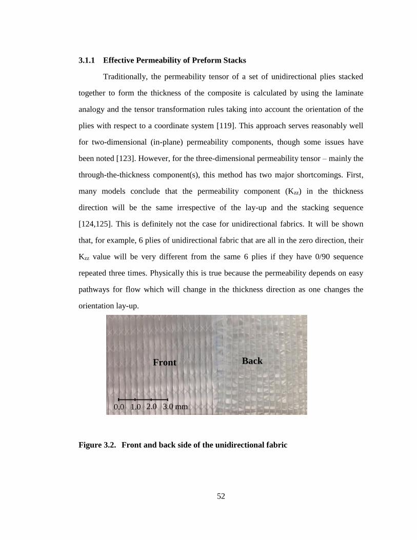
3.1.1 Effective Permeability of Preform Stacks ................................... 52
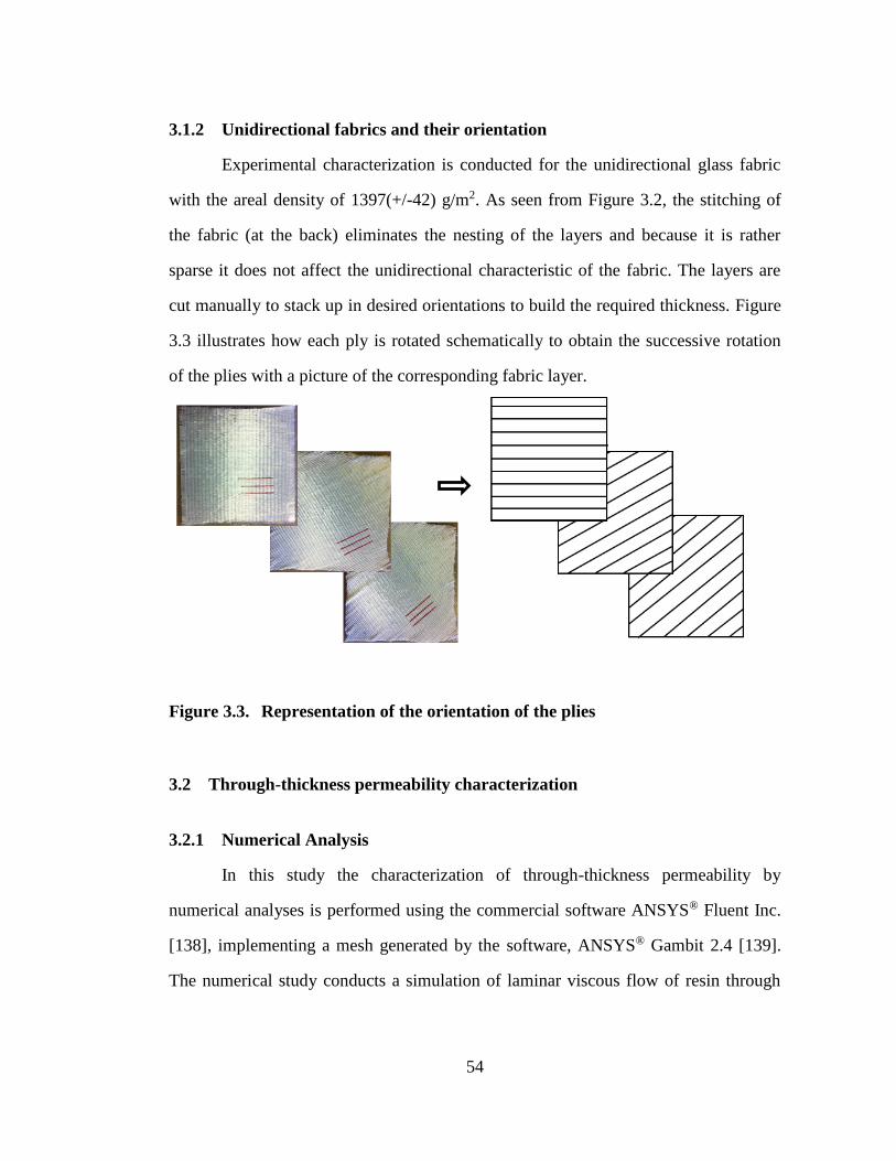
3.1.2 Unidirectional fabrics and their orientation ................................. 54
3.2 Through-thickness permeability characterization ................................... 54
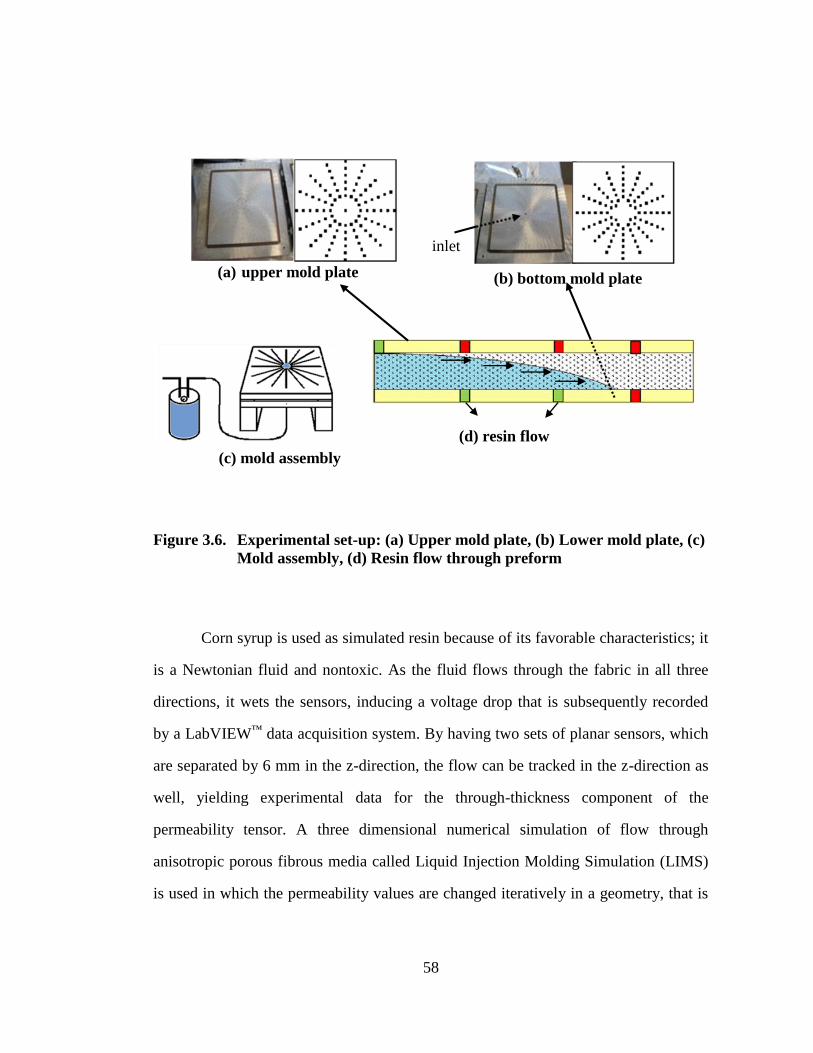
3.2.1 Numerical Analysis ..................................................................... 54 3.2.2 Experimental Validation .............................................................. 57
3.3 Results and Discussion ............................................................................ 59
3.3.1 Experimental Study ..................................................................... 59
3.3.2 Parametric Study ......................................................................... 61
3.4 Summary .................................................................................................. 65
4 CHARACTERIZATION OF LOCAL VARIABILITY OF FABRICS ........... 67
4.1 Introduction ............................................................................................. 67 4.2 Mathematical Implementation ................................................................. 70
4.3 Experimentation ...................................................................................... 77 4.4 Results and Discussion ............................................................................ 80
4.4.1 Characterization of permeability variation .................................. 80 4.4.2 Characterization of the defects within a fabric ............................ 83
4.5 Summary .................................................................................................. 87
5 OPTIMIZED DISTRIBUTION MEDIA LAYOUT ........................................ 88
5.1 Introduction ............................................................................................. 88
5.2 Flow Control Mechanisms for Flow Through Fibrous Domain .............. 88
Page 9
viii
5.3 Methodology and Implementation .......................................................... 90
5.3.1 Discrete Optimization .................................................................. 91
5.3.1.1 Tree Search Algorithms ................................................ 91
5.3.2 Pedagogical Example .................................................................. 93 5.3.3 Algorithm for Optimum DM lay-out ........................................... 97 5.3.4 Partition method .......................................................................... 98
5.4 Experimentation ...................................................................................... 99
5.5 Results and Discussion .......................................................................... 101
5.5.1 Experimental Validation ............................................................ 101 5.5.2 Complex Geometries ................................................................. 106
5.6 Summary ................................................................................................ 111
6 CONCLUSIONS, CONTRIBUTIONS AND FUTURE WORK .................. 112
6.1 Conclusions ........................................................................................... 112 6.2 Contributions of this work ..................................................................... 114
6.3 Future Work ........................................................................................... 116
REFERENCES ........................................................................................................... 118
Appendix
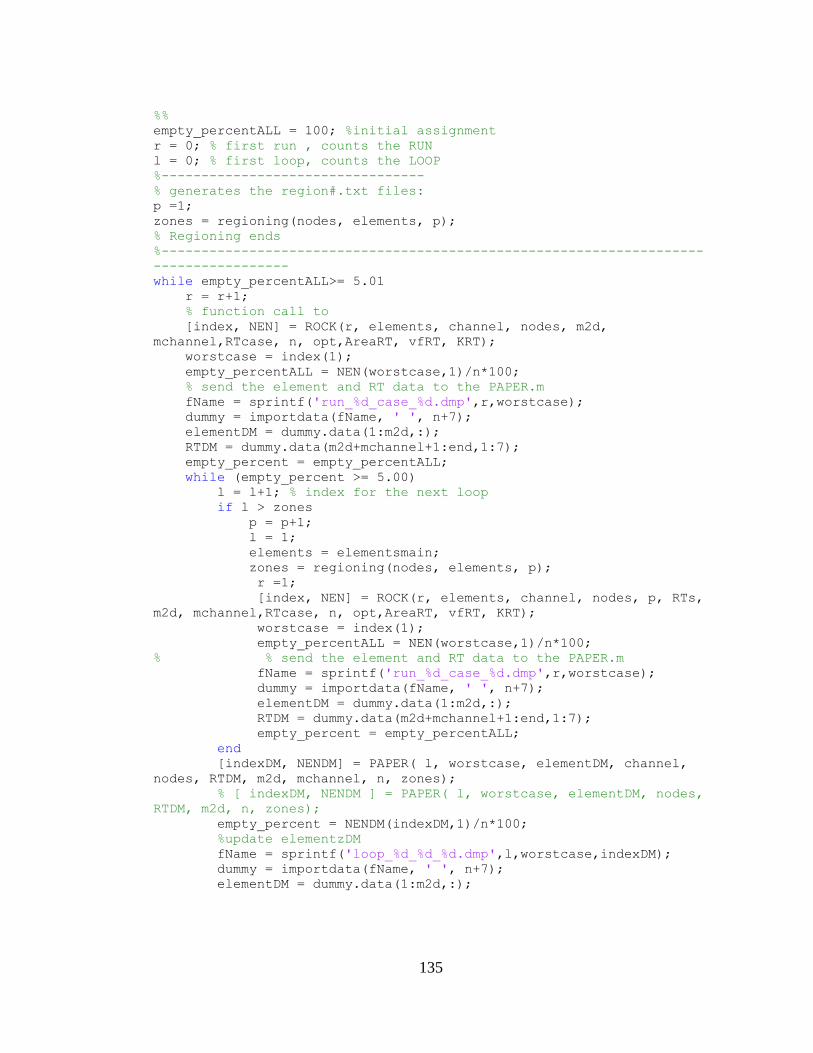
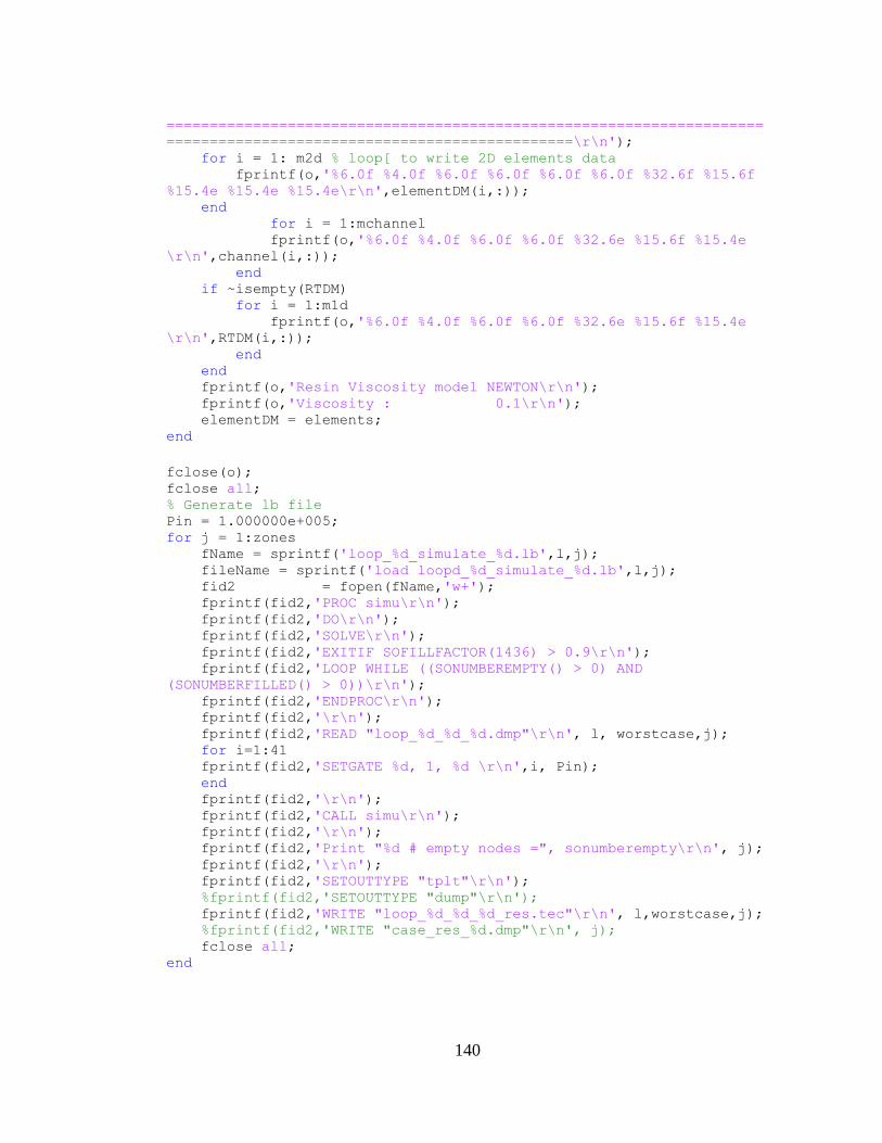
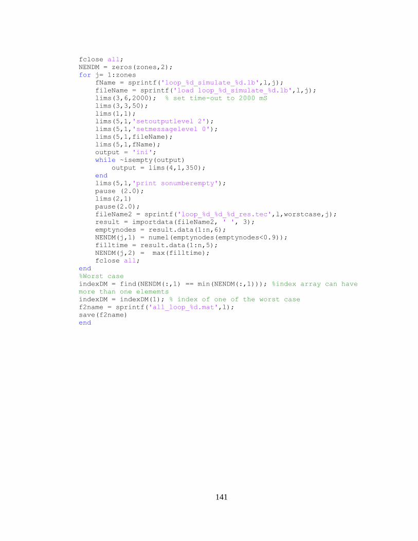
A MATLAB SCRIPTS FOR DISTRIBUTION MEDIA OPTIMIZATION ..... 132
A.1 Scissors.m: Main m-file ......................................................................... 133
A.2 Rock.m: Evaluation of all race-tracking possibilities ............................ 136
A.3 Paper.m: Finding the optimum region to place DM .............................. 138
B REPRINT PERMISSION LETTERS ............................................................. 142
B.1 “EFFECT OF RELATIVE PLY ORIENTATION ON THE
THROUGH-THICKNESS PERMEABILITY OF
UNIDIRECTIONAL FABRICS” .......................................................... 143
B.2 “FRACTAL CONCEPTS IN SURFACE GROWTH” ......................... 150
Page 10
ix
LIST OF TABLES
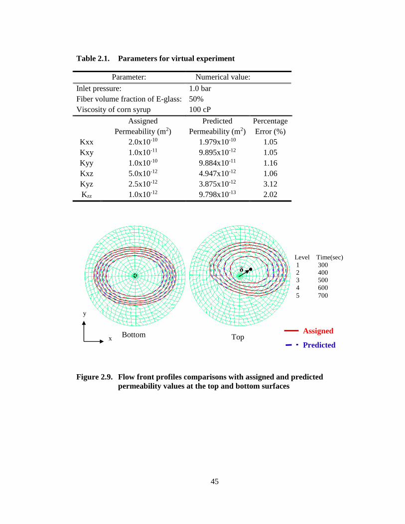
Table 2.1. Parameters for virtual experiment ........................................................... 45
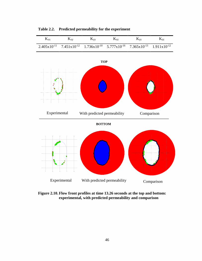
Table 2.2. Predicted permeability for the experiment .............................................. 46
Table 3.1. Experimental and numerical comparison of through-thickness
permeability. Case 1 and case 2 of 0o and 5o refers to all six
unidirectional layers being aligned along those angles respectively. In
case 3, case 4 and case 5, the successive layers were rotated by 5o,
45o and 90o degrees respectively. ........................................................... 60
Table 4.1. Characterization of the roughness exponent ........................................... 82
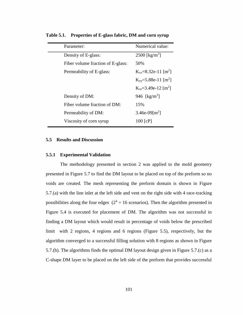
Table 5.1. Properties of E-glass fabric, DM and corn syrup .................................. 101
Page 11
x
LIST OF FIGURES
Figure 1.1. Type of reinforcements ............................................................................. 2
Figure 1.2. Different fabric types: (a) E-glass-plain weave, (b) E-glass random
mat, (c) Aramid twill weave, (d) Carbon twill weave ............................... 3
Figure 1.3. 3D reinforcement architectures (generated via TEXGEN [3]) ................. 4
Figure 1.4. Schematic of RTM (left) and VARTM (right) steps (adapted from [1]) .. 7
Figure 1.5. Schematic of SCRIMP steps ..................................................................... 9
Figure 1.6. Examples of (a) macro-void and (b) micro-void [27] ............................. 10
Figure 1.7. Example of defects in the preform; (a) plain weave glass fabric, (b)
3D orthogonal glass fabric ...................................................................... 11
Figure 1.8. Thickness variation during vacuum infusion .......................................... 13
Figure 1.9. Race-tracking formation on the edges due to fray edges ........................ 14
Figure 1.10. Race-tracking examples: (a) Mid-layer of the preform with metal
insert spatially in the middle, and Flow front profiles at the bottom of
the preform at two different time steps with race-tracking along the
metal insert for two same experimental configurations: (b) experiment
1, (c) experiment 2 ................................................................................... 15
Figure 1.11. Liquid Injection Molding Simulation (LIMS) Structure ......................... 18
Figure 1.12. Permeability map approach ..................................................................... 18
Figure 2.1. Flow front profile with xyz mold coordinate, x’y’z’ principle direction
of the preform .......................................................................................... 22
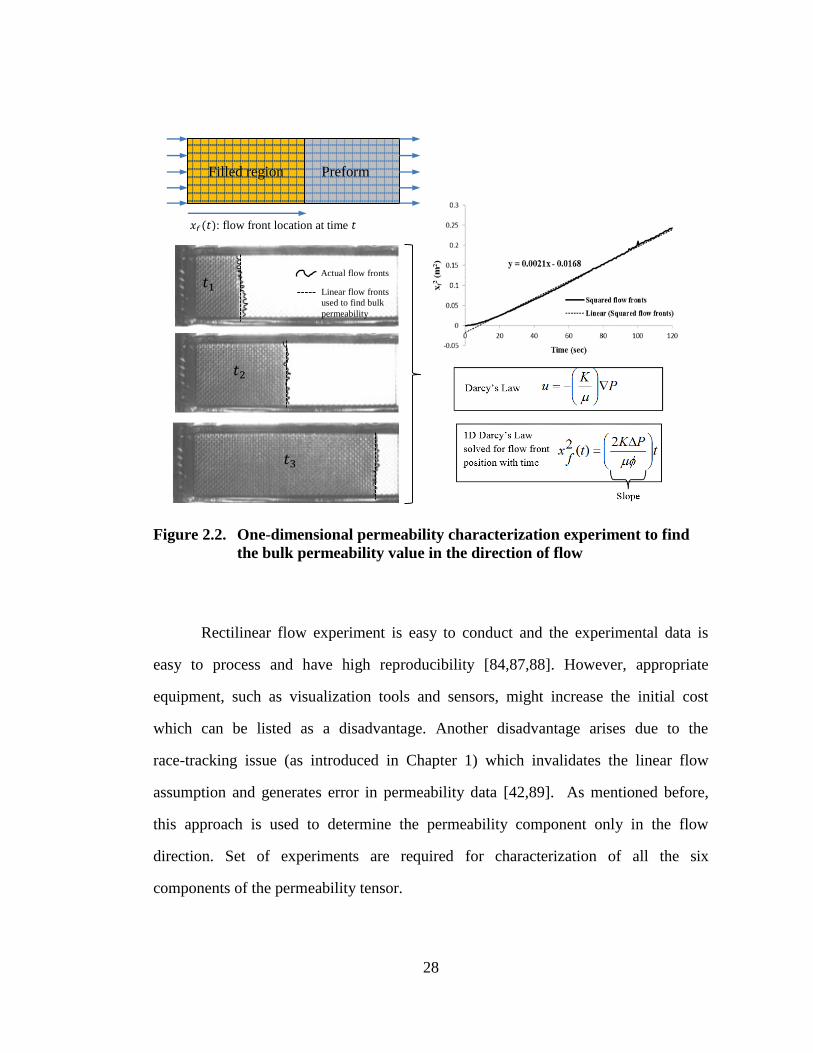
Figure 2.2. One-dimensional permeability characterization experiment to find the
bulk permeability value in the direction of flow ..................................... 28
Page 12
xi
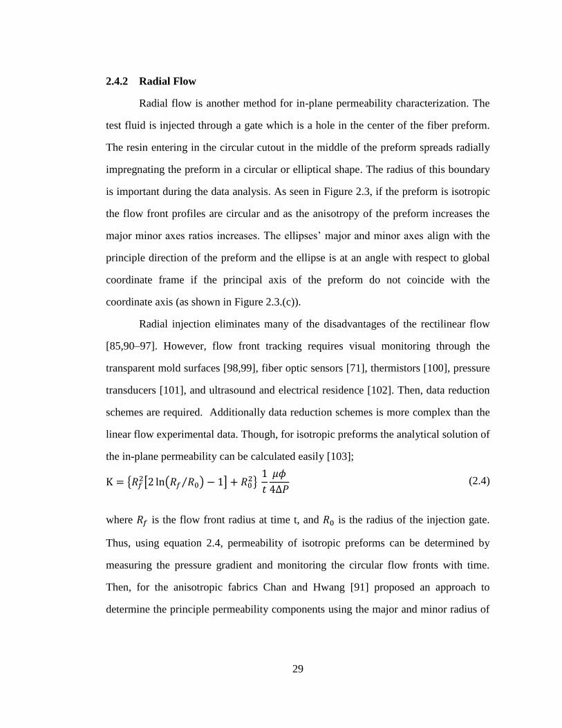
Figure 2.3. Schematic of radial flow front profiles: (a) isotropic (R1=R2), (b)
anisotropic (R1≠R2), (c) anisotropic with non-zero in-plane skew term
(global coordinate frame doesn’t coincides with principle directions of
the preform) ............................................................................................. 31
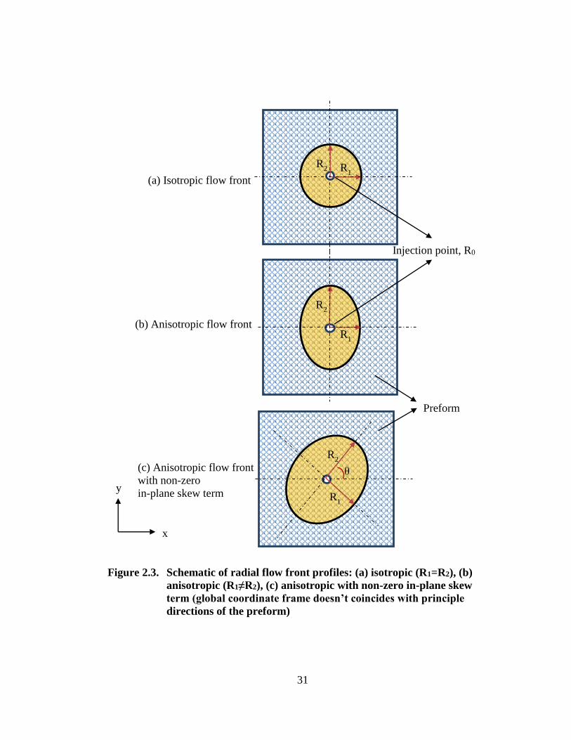
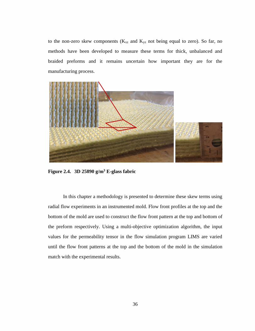
Figure 2.4. 3D 25890 g/m3 E-glass fabric ................................................................. 36
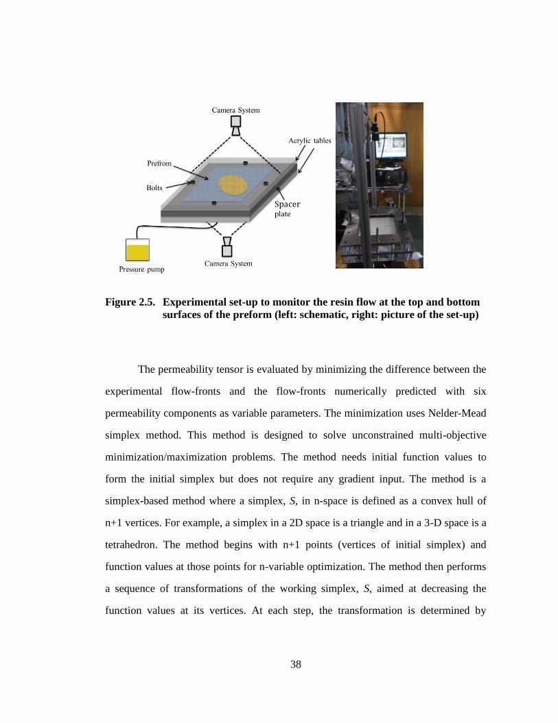
Figure 2.5. Experimental set-up to monitor the resin flow at the top and bottom
surfaces of the preform (left: schematic, right: picture of the set-up) ..... 38
Figure 2.6. (Left) An image of isotropic flow from an experiment. (Middle) The
image after having the preceding flow image subtracted from it,
filtered, and converted to binary. (Right) An ellipse is fitted to the
edge of the resin flow front. .................................................................... 39
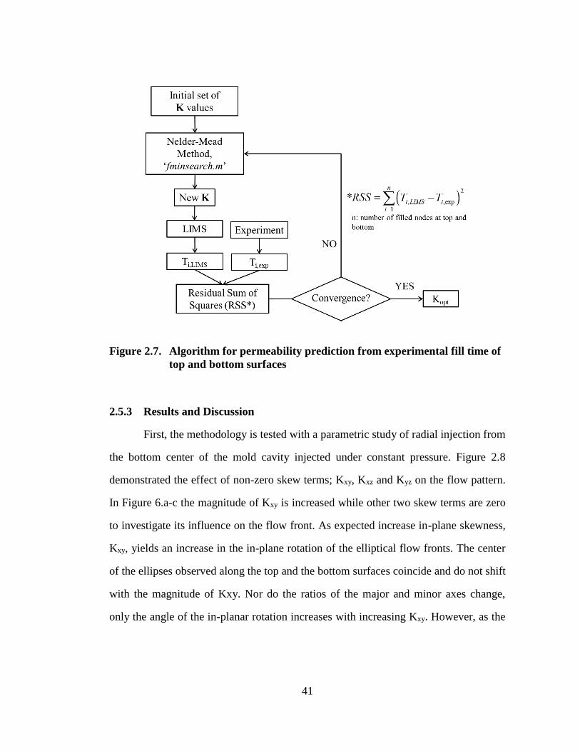
Figure 2.7. Algorithm for permeability prediction from experimental fill time of
top and bottom surfaces ........................................................................... 41
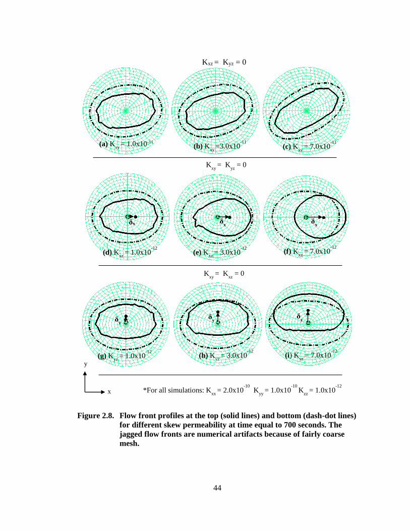
Figure 2.8. Flow front profiles at the top (solid lines) and bottom (dash-dot lines)
for different skew permeability at time equal to 700 seconds. The
jagged flow fronts are numerical artifacts because of fairly coarse
mesh. ........................................................................................................ 44
Figure 2.9. Flow front profiles comparisons with assigned and predicted
permeability values at the top and bottom surfaces ................................ 45
Figure 2.10. Flow front profiles at time 13.26 seconds at the top and bottom:
experimental, with predicted permeability and comparison ................... 46
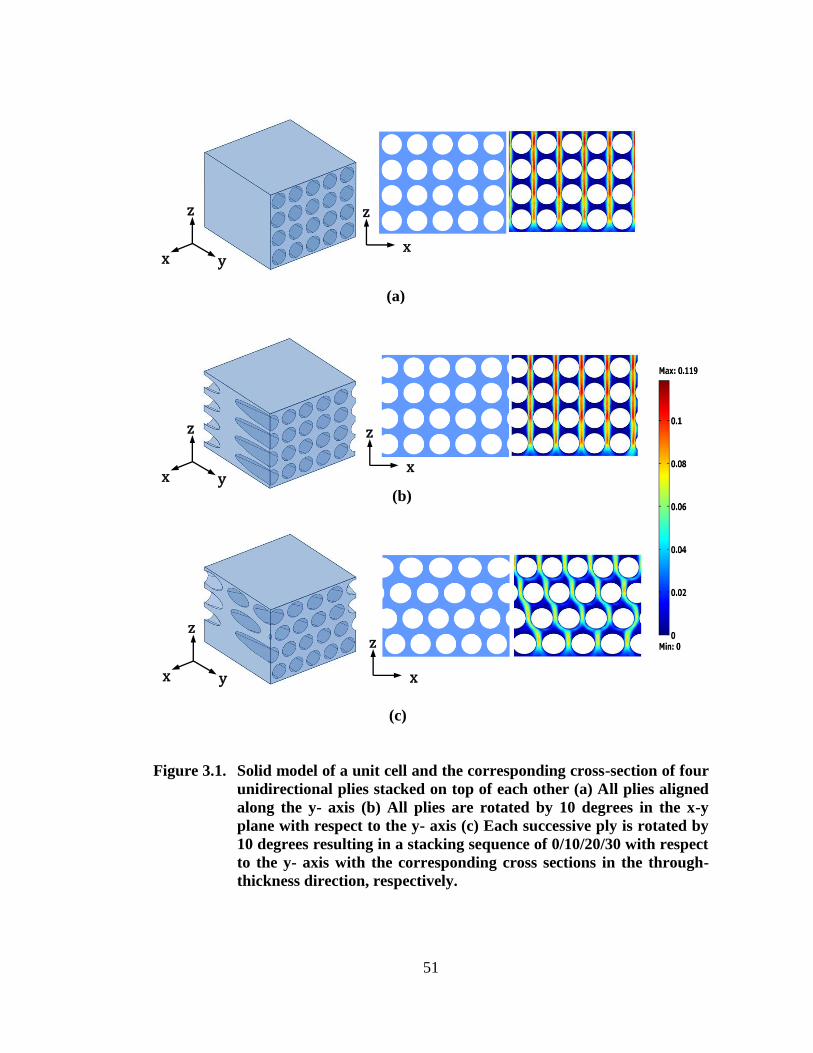
Figure 3.1. Solid model of a unit cell and the corresponding cross-section of four
unidirectional plies stacked on top of each other (a) All plies aligned
along the y- axis (b) All plies are rotated by 10 degrees in the x-y
plane with respect to the y- axis (c) Each successive ply is rotated by
10 degrees resulting in a stacking sequence of 0/10/20/30 with respect
to the y- axis with the corresponding cross sections in the through-
thickness direction, respectively. ............................................................. 51
Figure 3.2. Front and back side of the unidirectional fabric ...................................... 52
Figure 3.3. Representation of the orientation of the plies .......................................... 54
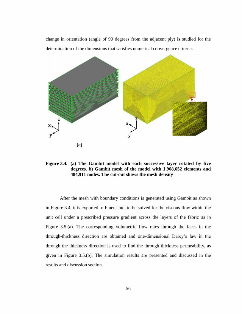
Figure 3.4. (a) The Gambit model with each successive layer rotated by five
degrees. b) Gambit mesh of the model with 1,968,652 elements and
484,911 nodes. The cut-out shows the mesh density .............................. 56
Page 13
xii
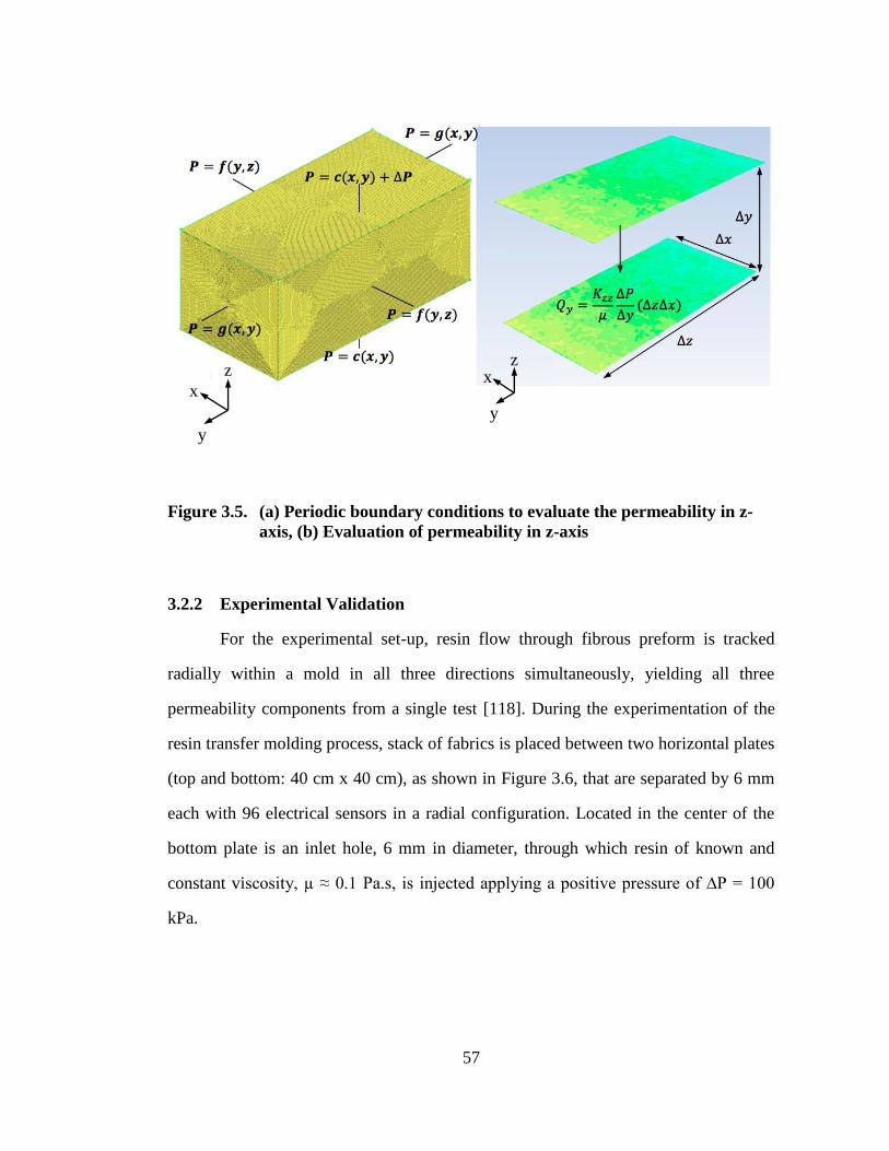
Figure 3.5. (a) Periodic boundary conditions to evaluate the permeability in z-
axis, (b) Evaluation of permeability in z-axis ......................................... 57
Figure 3.6. Experimental set-up: (a) Upper mold plate, (b) Lower mold plate, (c)
Mold assembly, (d) Resin flow through preform .................................... 58
Figure 3.7. Numerical through thickness permeability with different mesh
element sizes for incremental rotation angle 5o ....................................... 61
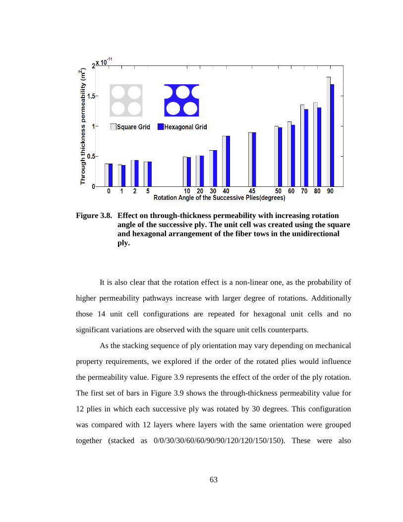
Figure 3.8. Effect on through-thickness permeability with increasing rotation
angle of the successive ply. The unit cell was created using the square
and hexagonal arrangement of the fiber tows in the unidirectional ply. . 63
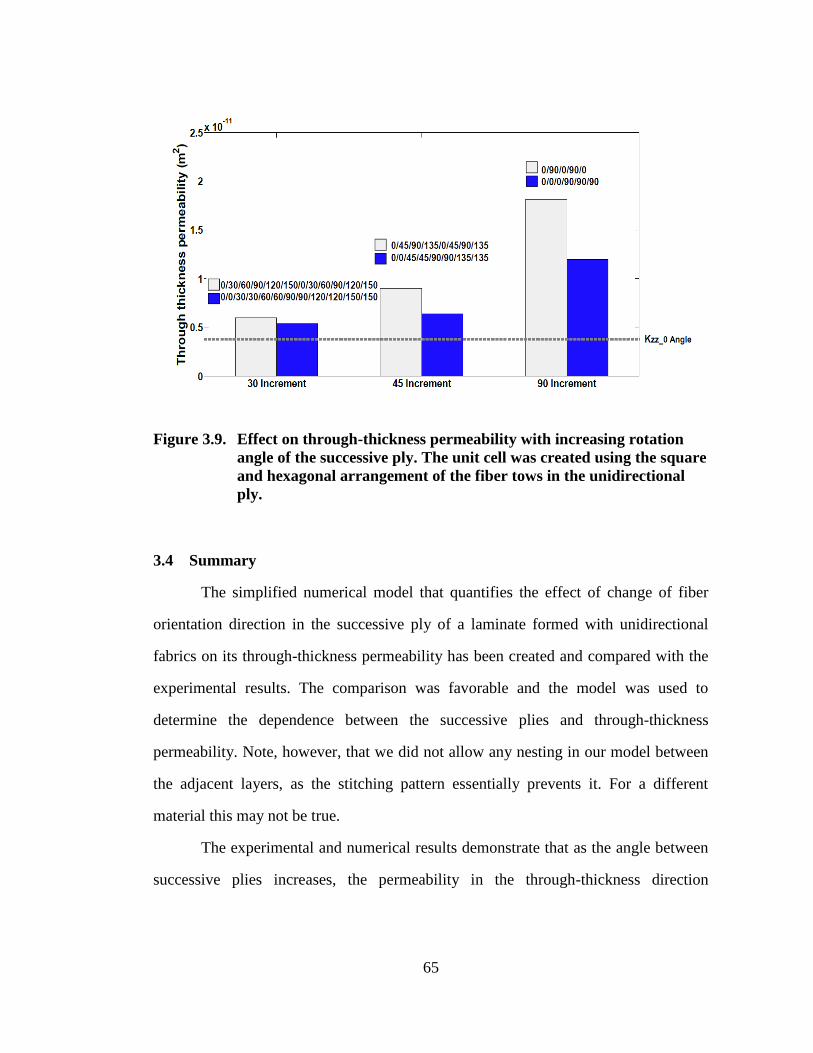
Figure 3.9. Effect on through-thickness permeability with increasing rotation
angle of the successive ply. The unit cell was created using the square
and hexagonal arrangement of the fiber tows in the unidirectional ply. . 65
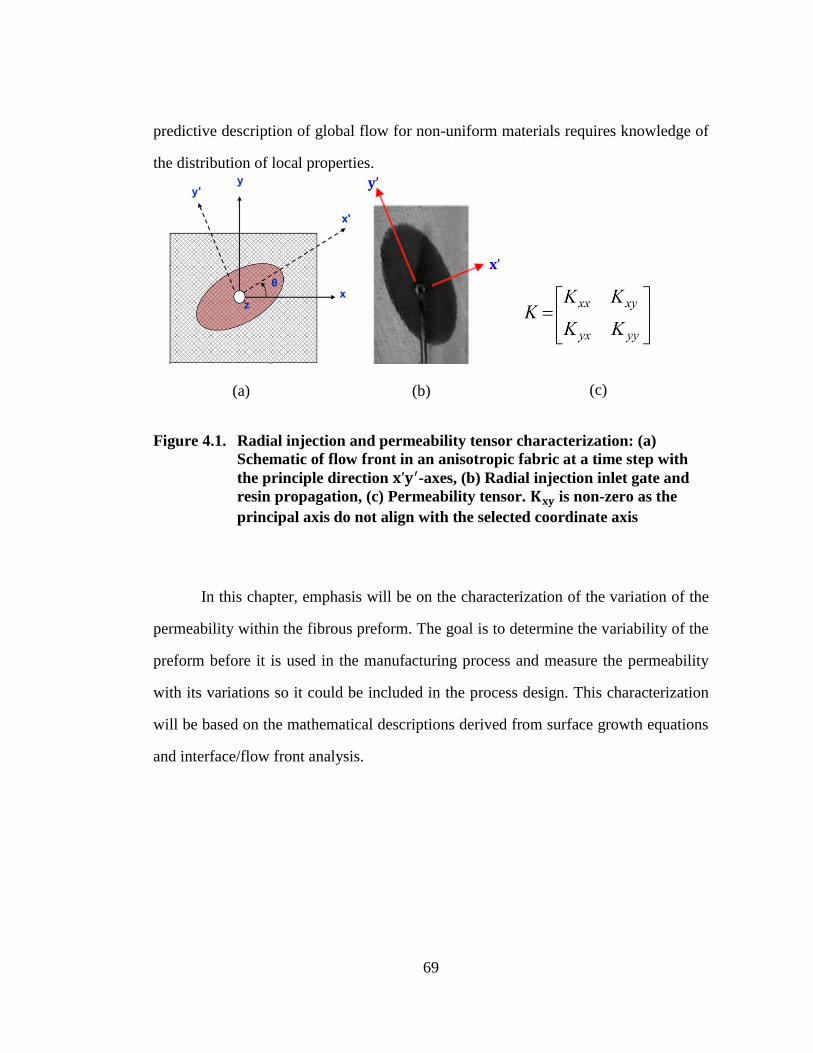
Figure 4.1. Radial injection and permeability tensor characterization: (a)
Schematic of flow front in an anisotropic fabric at a time step with the
principle direction 𝐱’𝐲′-axes, (b) Radial injection inlet gate and resin
propagation, (c) Permeability tensor. 𝐊𝐱𝐲 is non-zero as the principal
axis do not align with the selected coordinate axis ................................. 69
Figure 4.2. Flow front locations (height 𝐡(𝐫, 𝐭)) at various times with system size
L, and mean height (flow front position) 𝒉 ............................................. 70
Figure 4.3. (a) Change of the interface width with time (logarithmic scales for
both axes) for a fixed L value , (b) Growth of the interface width with
different system sizes (L). Reprinted with permission from [143] ......... 71
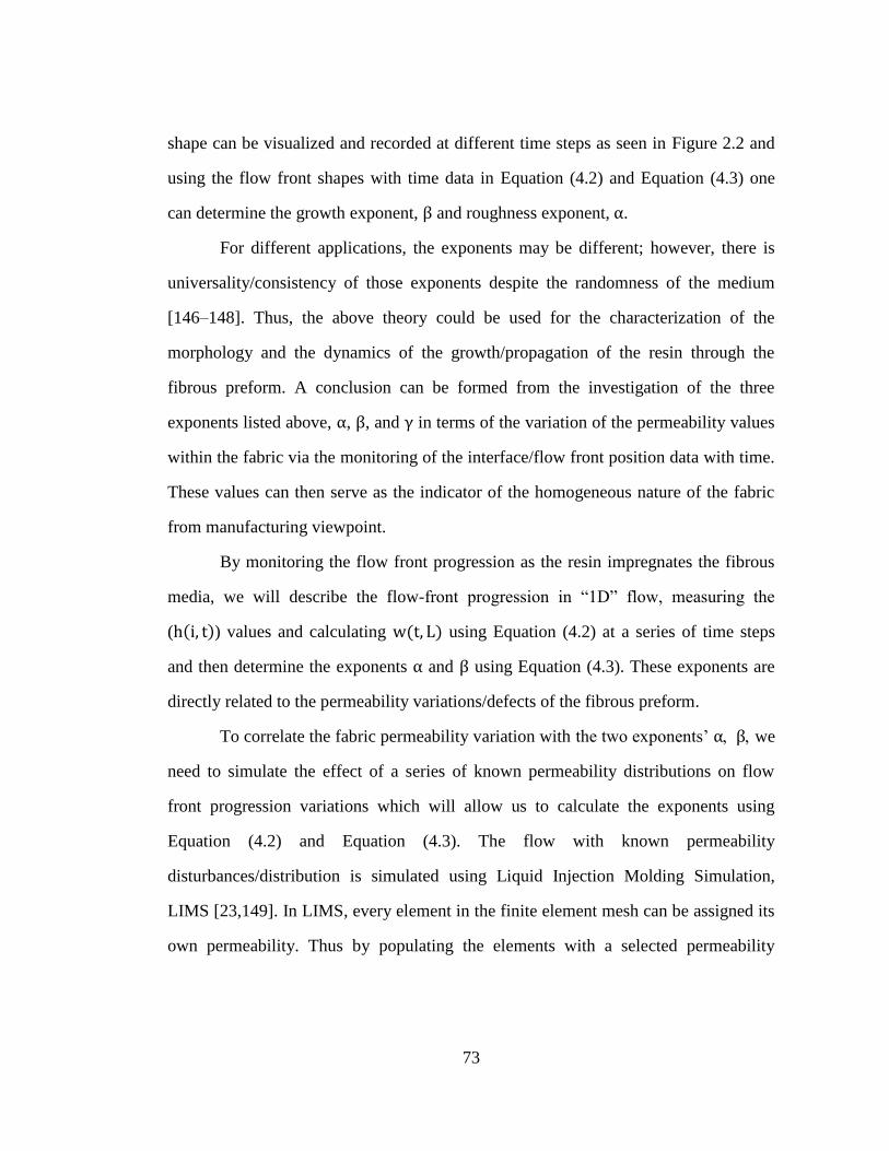
Figure 4.4. Top: LIMS mesh and random permeability assignment, Bottom: flow
front progression with time obtained via LIMS ...................................... 75
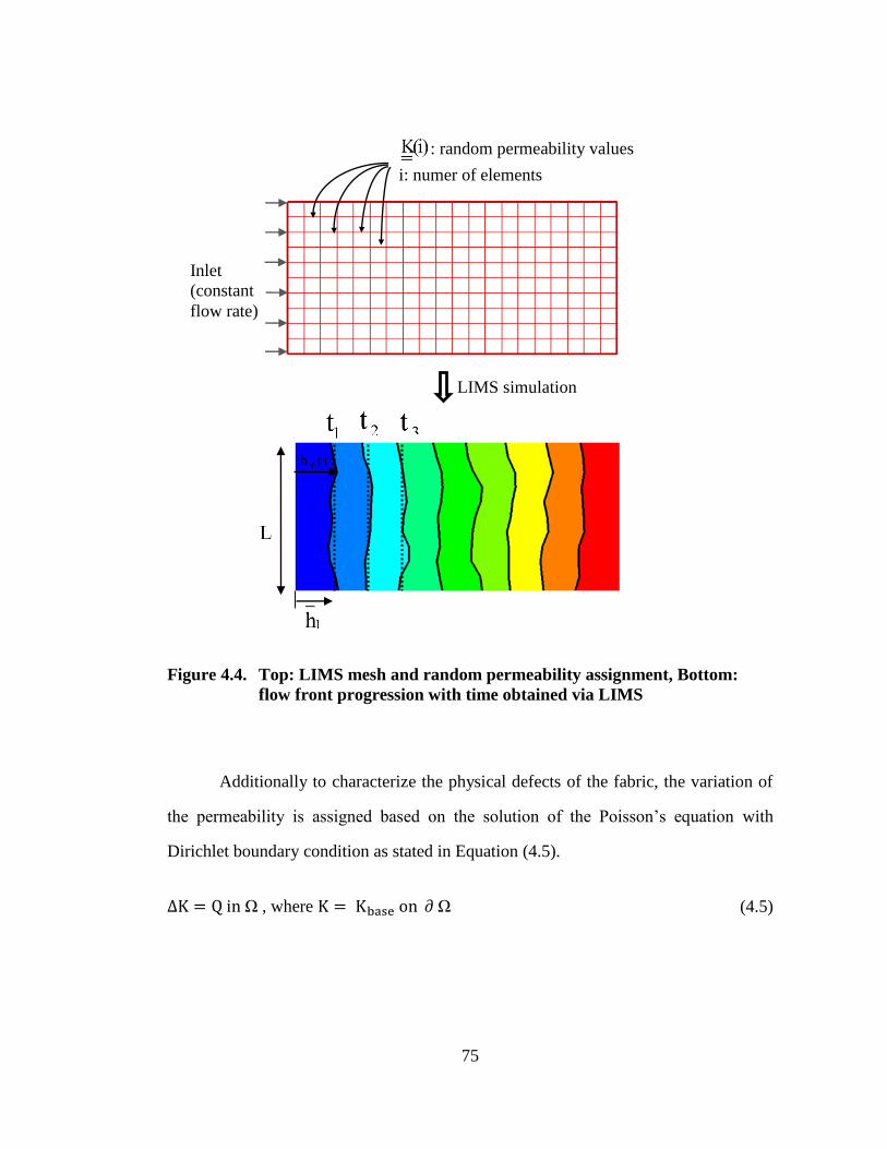
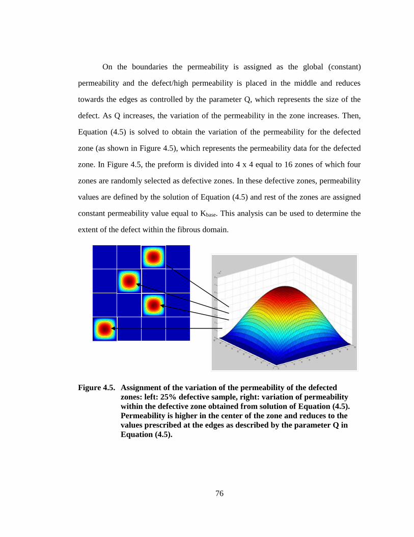
Figure 4.5. Assignment of the variation of the permeability of the defected zones:
left: 25% defective sample, right: variation of permeability within the
defective zone obtained from solution of Equation (4.5). Permeability
is higher in the center of the zone and reduces to the values prescribed
at the edges as described by the parameter Q in Equation (4.5). ............ 76
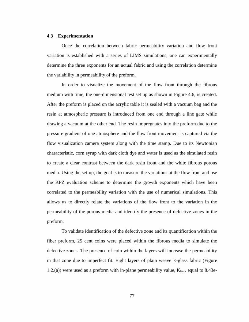
Figure 4.6. Flow through porous media experimental set-up with flow
visualization ............................................................................................. 78
Page 14
xiii
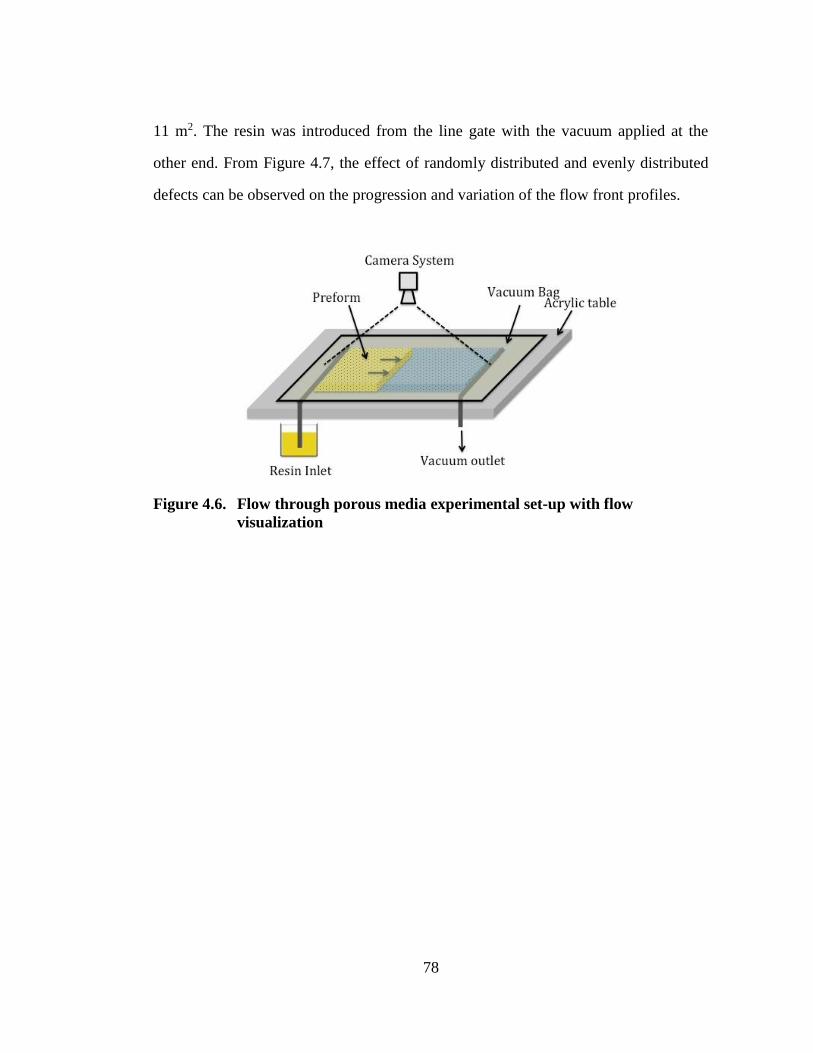
Figure 4.7. Resin flowing into a fibrous preform with 25 cent coins placed inside
the fabric to simulate defective regions. On the left the defects were
evenly distributed on the right the defects are randomly distributed.
Measured experimental flow front profiles are also shown (flow front
contours at Δt = 25 seconds) ................................................................... 79
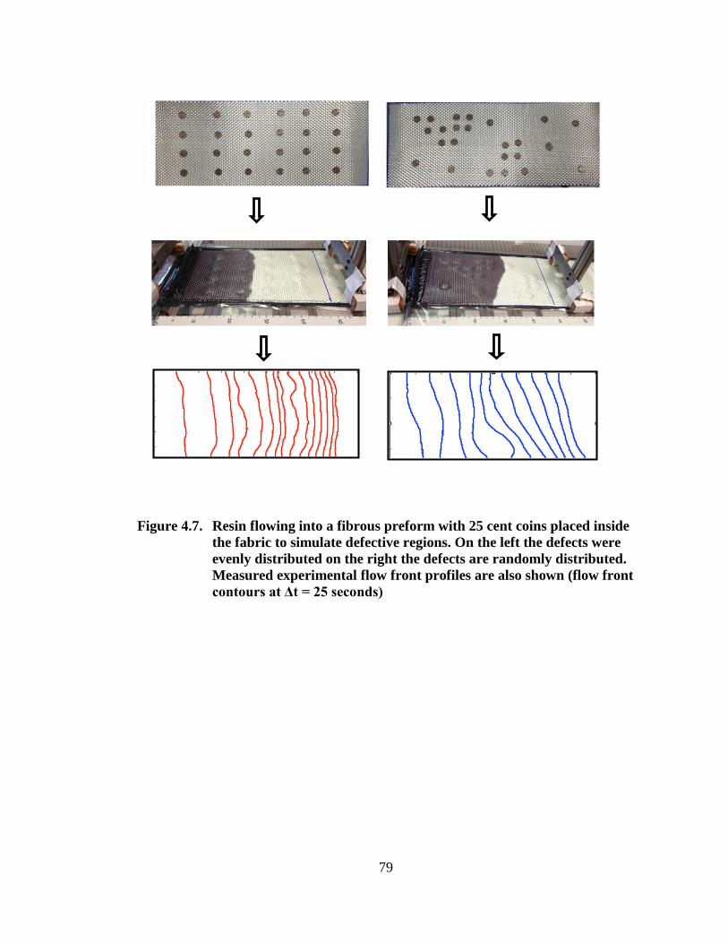
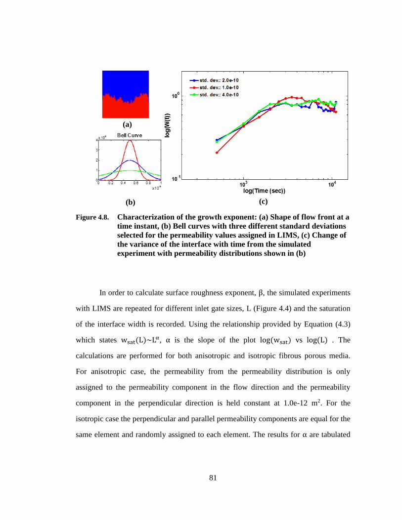
Figure 4.8. Characterization of the growth exponent: (a) Shape of flow front at a
time instant, (b) Bell curves with three different standard deviations
selected for the permeability values assigned in LIMS, (c) Change of
the variance of the interface with time from the simulated experiment
with permeability distributions shown in (b) .......................................... 81
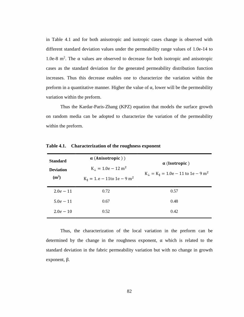
Figure 4.9. Change in growth exponent, 𝛃 with increasing percentage of defective
zones (m) for different degree of defects, Q. A best fit functional
relationship is also plotted ....................................................................... 84
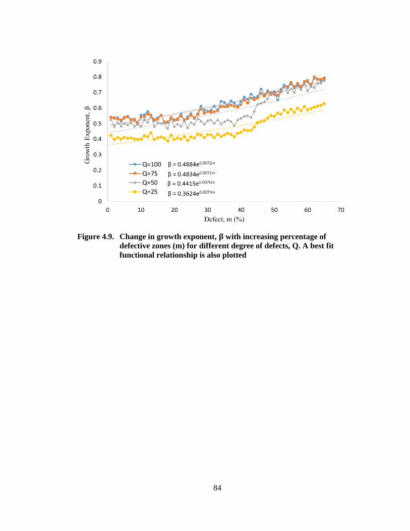
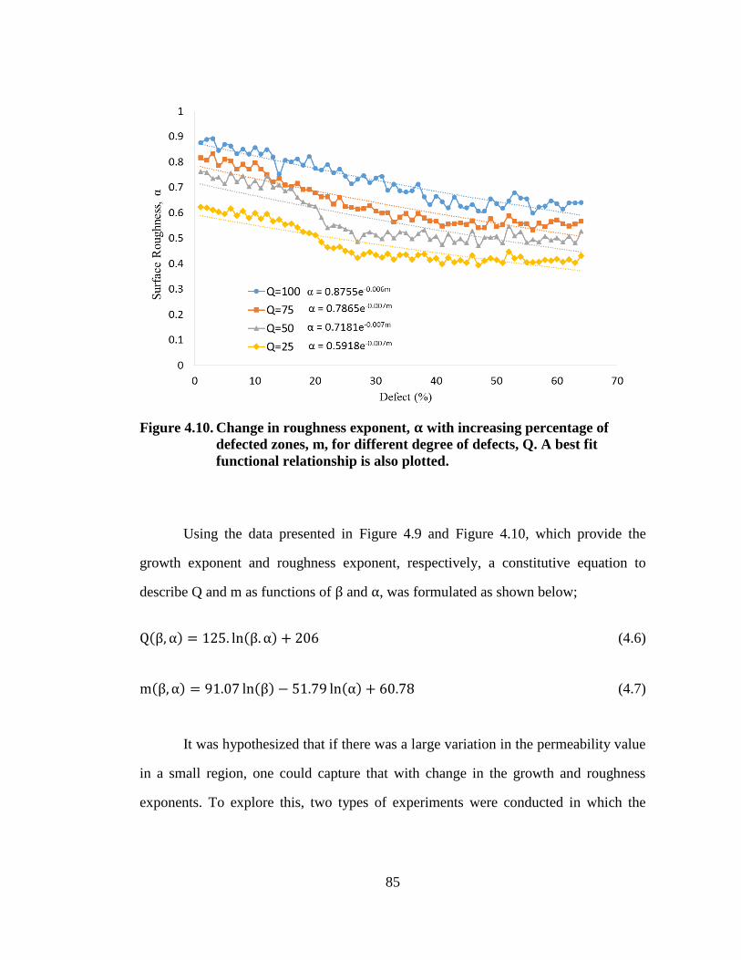
Figure 4.10. Change in roughness exponent, 𝛂 with increasing percentage of
defected zones, m, for different degree of defects, Q. A best fit
functional relationship is also plotted. ..................................................... 85
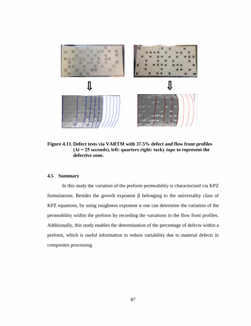
Figure 4.11. Defect tests via VARTM with 37.5% defect and flow front profiles
(Δt = 25 seconds), left: quarters right: tacky tape to represent the
defective zone. ......................................................................................... 87
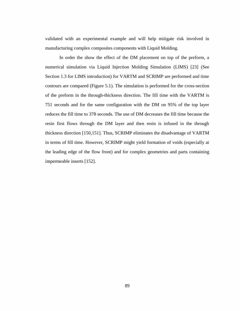
Figure 5.1. Fill time contours for a VARTM and SCRIMP ...................................... 90
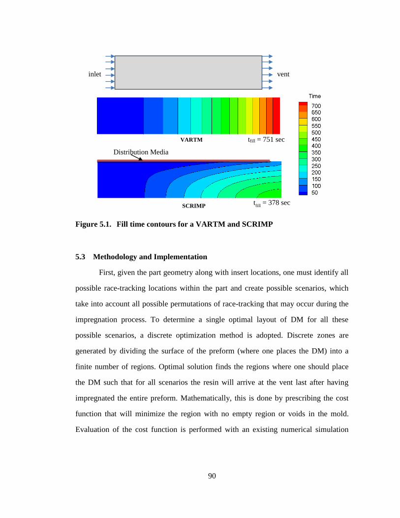
Figure 5.2. Tree search algorithms (a) example problem with two acceptable, H
and T, nodes, (b) Breadth-first search: finds node H, (c) Depth-first
search: finds node T ................................................................................ 92
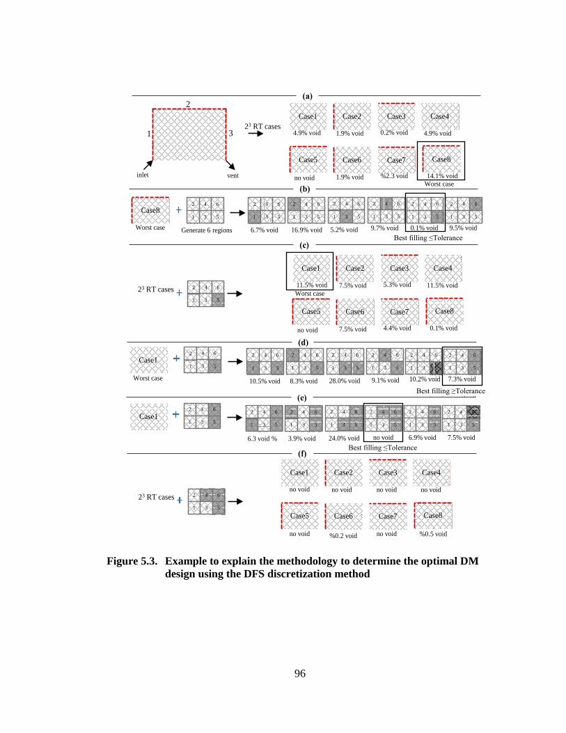
Figure 5.3. Example to explain the methodology to determine the optimal DM
design using the DFS discretization method ........................................... 96
Figure 5.4. Flow chart of the algorithm to obtain optimal DM ................................. 98
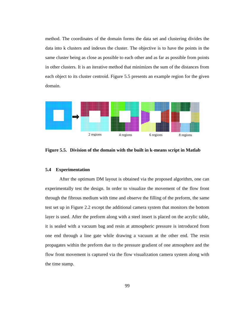
Figure 5.5. Division of the domain with the built in k-means script in Matlab ......... 99
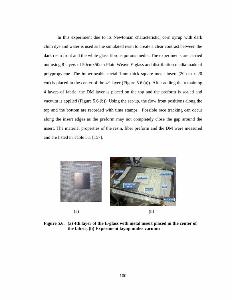
Figure 5.6. (a) 4th layer of the E-glass with metal insert placed in the center of the
fabric, (b) Experiment layup under vacuum .......................................... 100
Page 15
xiv
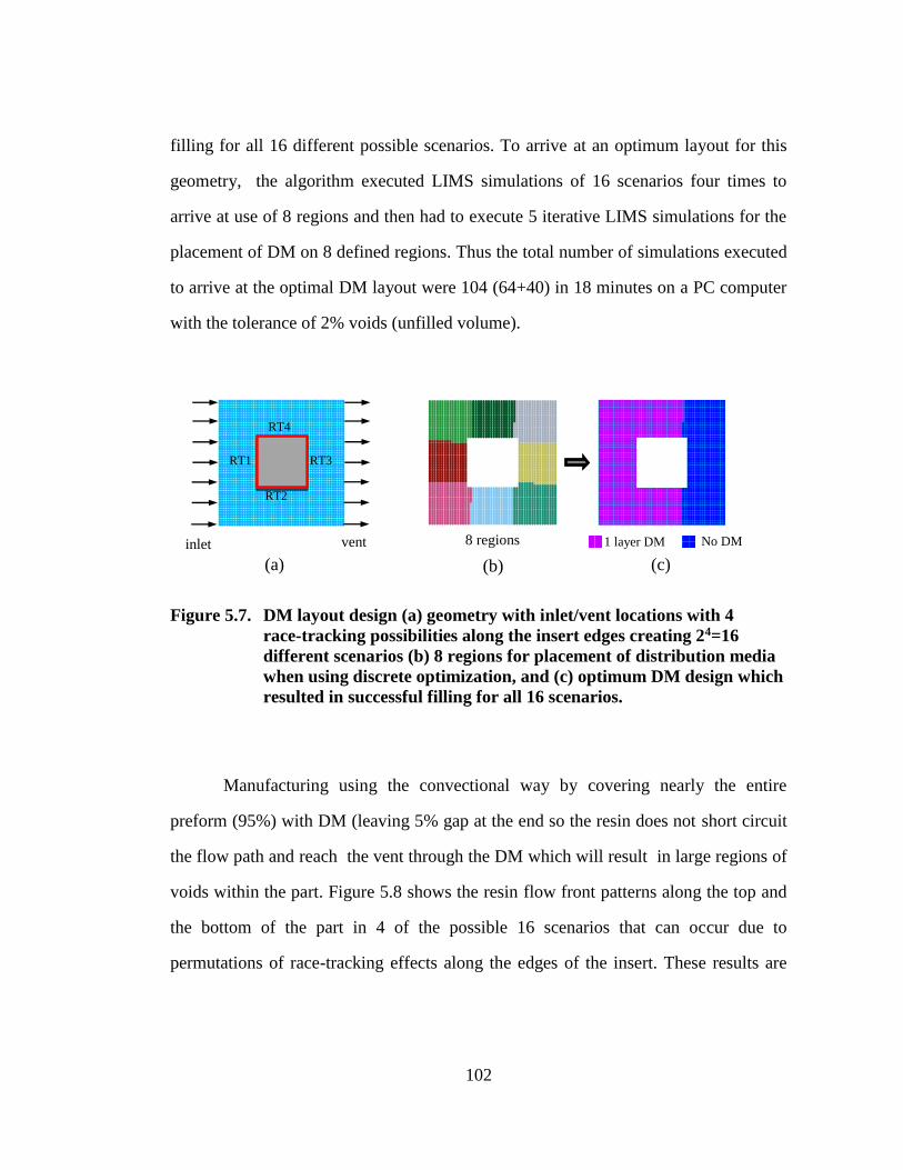
Figure 5.7. DM layout design (a) geometry with inlet/vent locations with 4
race-tracking possibilities along the insert edges creating 24=16
different scenarios (b) 8 regions for placement of distribution media
when using discrete optimization, and (c) optimum DM design which
resulted in successful filling for all 16 scenarios. ................................. 102
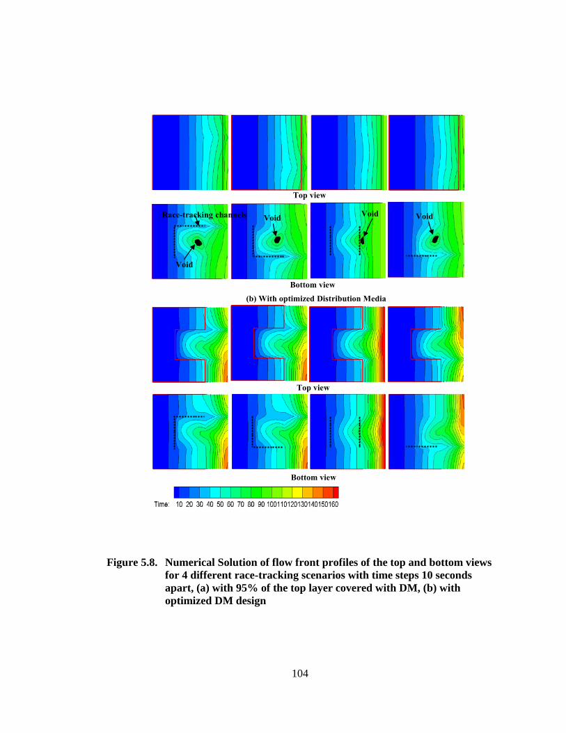
Figure 5.8. Numerical Solution of flow front profiles of the top and bottom views
for 4 different race-tracking scenarios with time steps 10 seconds
apart, (a) with 95% of the top layer covered with DM, (b) with
optimized DM design ............................................................................ 104
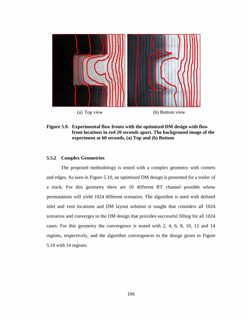
Figure 5.9. Experimental flow fronts with the optimized DM design with flow
front locations in red 20 seconds apart. The background image of the
experiment at 60 seconds, (a) Top and (b) Bottom ............................... 106
Figure 5.10. Optimized DM design of trailer geometry with 1024 different possible
flow patterns .......................................................................................... 107
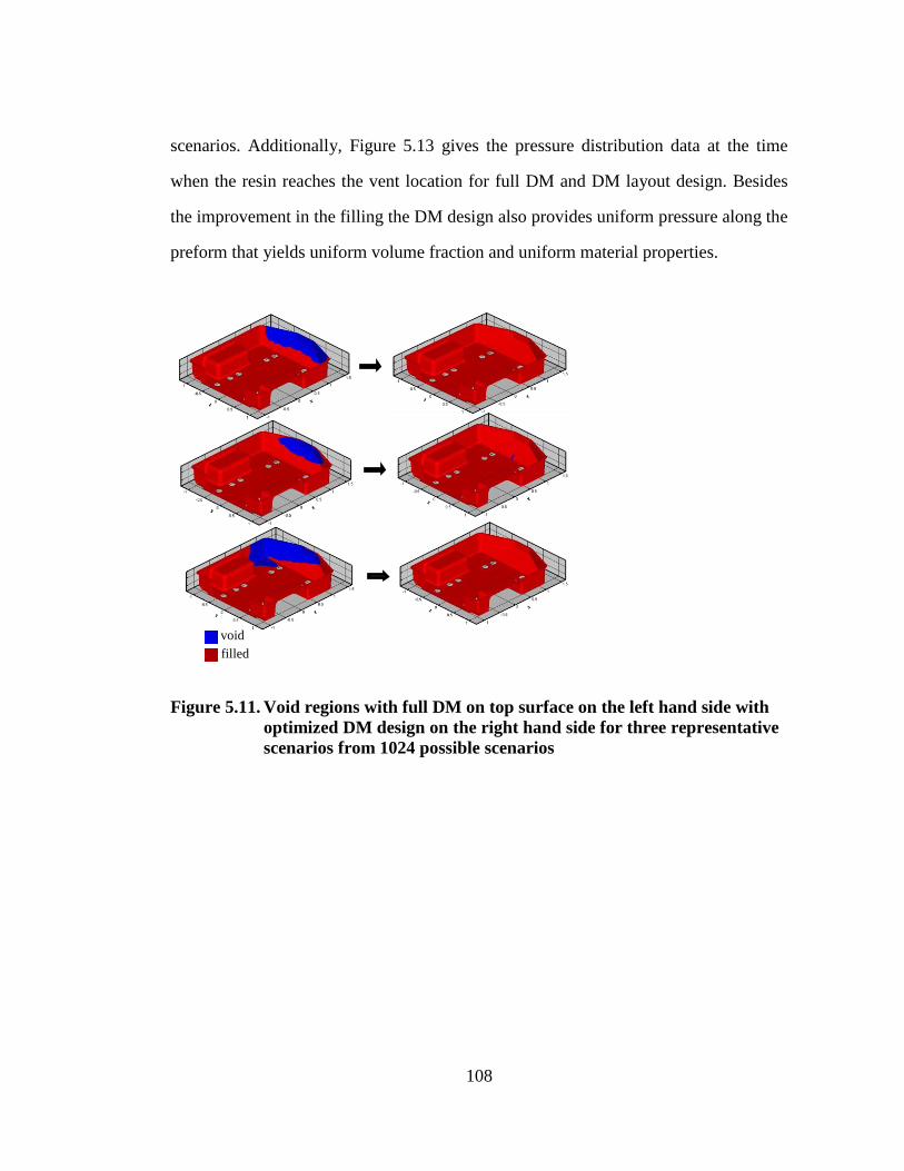
Figure 5.11. Void regions with full DM on top surface on the left hand side with
optimized DM design on the right hand side for three representative
scenarios from 1024 possible scenarios ................................................ 108
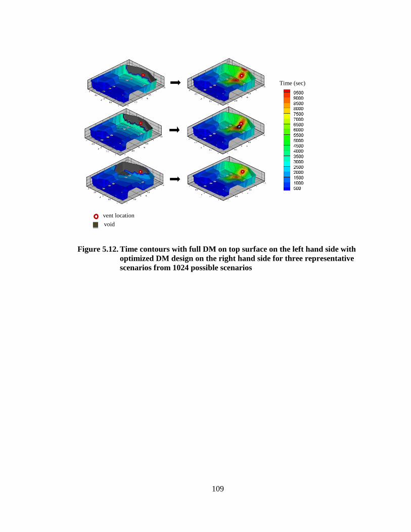
Figure 5.12. Time contours with full DM on top surface on the left hand side with
optimized DM design on the right hand side for three representative
scenarios from 1024 possible scenarios ................................................ 109
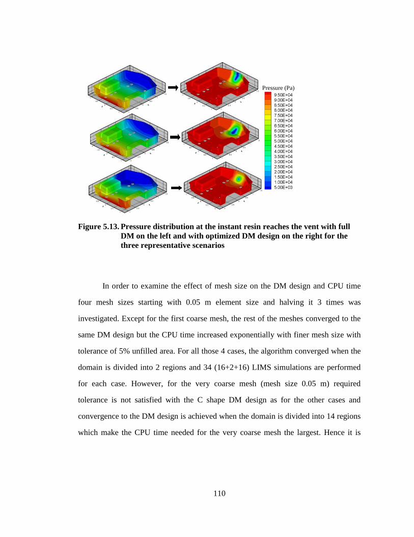
Figure 5.13. Pressure distribution at the instant resin reaches the vent with full DM
on the left and with optimized DM design on the right for the three
representative scenarios ......................................................................... 110
Figure 5.14. Change in CPU time with mesh size for optimized DM design ........... 111
Page 16
xv
ABSTRACT
In Liquid Composite Molding (LCM) processes, reinforcing glass, carbon or
Kevlar fiber preforms are placed in a mold cavity and a liquid resin is introduced to
cover the remaining empty space to form a composite by curing the resin. The fiber
preform permeability plays a key role in the filling pattern of the mold, which dictates
if there will be any voids (empty spaces) in the composite. Permeability tensor
describes the resistance to fluid flow through the anisotropic fibrous porous media,
which may not be spatially uniform. The variability in the permeability due to the
variation in the preform or its placement in the mold can influence the filling pattern
and hence the quality of the part being manufactured. The permeability map of a
preform specifies the values of components of the permeability tensor at various
locations of the preform. The overall objective of this dissertation is to investigate
various approaches and tools to create a permeability map that will ensure filling to
achieve manufacturing success despite the variability of the filling pattern, a
requirement of robust process design.
When unidirectional fabrics are used to manufacture composites, they are
typically stacked on top of each other to build up the desired thickness. A slight
misalignment during the stacking can change the through-thickness permeability
dramatically and the flow pattern due to the creation of low-resistance pathways.
Experimental characterization of the out-of-plane or through-thickness permeability of
a series of unidirectional fabrics stacked in various orientations is investigated. Also,
numerical simulations are conducted to predict the effect of change in fiber orientation
Page 17
xvi
on the through-thickness permeability for unidirectional fabrics. Results demonstrate
that the stacking sequence of the unidirectional fabrics influence the through thickness
flow and hence the transverse permeability.
Next, variation in the permeability value of the fibrous domain caused by the
non-uniformity in fiber architecture is investigated. The time evolution and geometry
of the rough interfaces of the fluid flow in porous medium are analyzed using the
concepts of dynamic scaling and self-affine fractal geometry and is shown to belong to
the Kardar-Parisi-Zhang (KPZ) universality class. Additionally, this characterization
can be used to quantify the percentage of abnormalities within the preform from flow
front profile analysis using KPZ formulation.
Finally, a methodology is introduced to create a permeability map for a given
mold geometry along with inlet and vent locations which will allow the mold to
completely fill despite the variations in the preform and the flow disturbances caused
due to its placement. The resin flow pattern can be manipulated with a tailored highly
permeable layer (Distribution Media (DM)) layout to be placed on top of the preform
as it does impact the flow patterns significantly. Thus, a predictive tool to design an
optimal shape of DM, which accounts for the flow variability introduced due to
race-tracking along the edges of the inserts is presented by adapting a discrete
optimization algorithm.
Page 18
1
Chapter 1
INTRODUCTION
1.1 Liquid Composite Molding
Polymer composite materials combine polymeric resin with reinforcing fibers
to fabricate products that are lightweight of tailored stiffness and strength with
improved fatigue life and corrosion resistance compared to traditional materials. There
are various manufacturing methods to combine the reinforcement and matrix materials
together. Injection molding, hand lay-up, filament winding, pultrusion, compression
molding of sheet molding compound (SMC), prepreg vacuum bagging and autoclave
curing and liquid composite molding (LCM) to name a few commonly employed
processes. Selection of the manufacturing method is mainly based on the geometrical
and structural properties constraints in addition to total volume and cost requirements.
For example, one should use filament winding for making composite pressure tanks
and pultrusion for long profiles such as poles and window frames. Moreover, the
manufacturing method should result in desired design properties with low cost and
cycle time.
LCM is one of the most popular manufacturing method for its short cycle
times, low cost, high quality and it can handle complex geometries. LCM is a class of
processes in which the dry fiber preform in the shape of final product is placed in a
mold and impregnated by the desired resin system. The types of materials and the
common processes that belong to this family are described in the following sections.
Page 19
2
1.1.1 Materials used in LCM
The process design of the LCM starts with the selection of the reinforcement
and the resin system that can satisfy the design requirements.
1.1.1.1 Reinforcements
High strength and high stiffness reinforcements are the load carriers of the
composite materials and usually manufactured as continuous fibers. These continuous
fibers can be put together in the form of rovings, yarns, strands and tows [1]. Different
forms of yarns or tows (bundles of fibers) can be used to create fiber preforms. Fabric
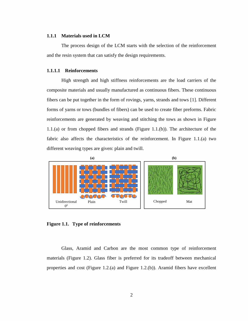
reinforcements are generated by weaving and stitching the tows as shown in Figure
1.1.(a) or from chopped fibers and strands (Figure 1.1.(b)). The architecture of the
fabric also affects the characteristics of the reinforcement. In Figure 1.1.(a) two
different weaving types are given: plain and twill.
Figure 1.1. Type of reinforcements
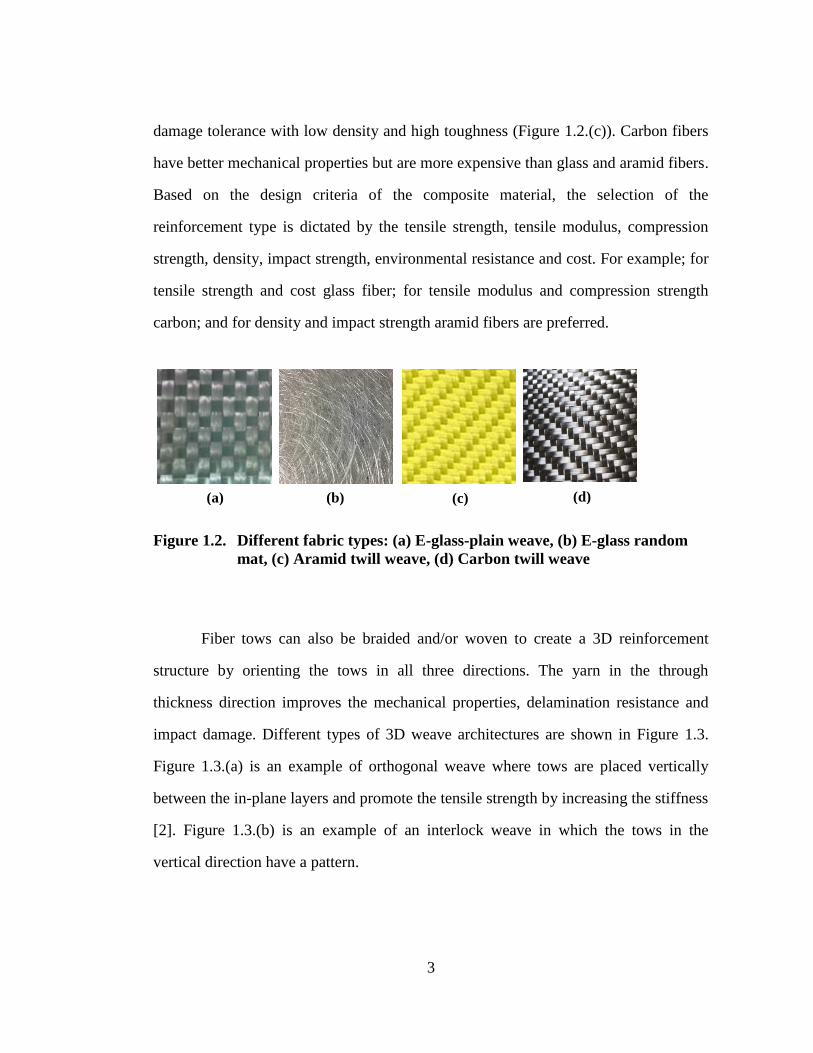
Glass, Aramid and Carbon are the most common type of reinforcement
materials (Figure 1.2). Glass fiber is preferred for its tradeoff between mechanical
properties and cost (Figure 1.2.(a) and Figure 1.2.(b)). Aramid fibers have excellent
Unidirectional
00
Plain
(a) (b)
Twill Chopped Mat
Page 20
3
damage tolerance with low density and high toughness (Figure 1.2.(c)). Carbon fibers
have better mechanical properties but are more expensive than glass and aramid fibers.
Based on the design criteria of the composite material, the selection of the
reinforcement type is dictated by the tensile strength, tensile modulus, compression
strength, density, impact strength, environmental resistance and cost. For example; for
tensile strength and cost glass fiber; for tensile modulus and compression strength
carbon; and for density and impact strength aramid fibers are preferred.
Figure 1.2. Different fabric types: (a) E-glass-plain weave, (b) E-glass random
mat, (c) Aramid twill weave, (d) Carbon twill weave
Fiber tows can also be braided and/or woven to create a 3D reinforcement
structure by orienting the tows in all three directions. The yarn in the through
thickness direction improves the mechanical properties, delamination resistance and
impact damage. Different types of 3D weave architectures are shown in Figure 1.3.
Figure 1.3.(a) is an example of orthogonal weave where tows are placed vertically
between the in-plane layers and promote the tensile strength by increasing the stiffness
[2]. Figure 1.3.(b) is an example of an interlock weave in which the tows in the
vertical direction have a pattern.
(a) (b) (c) (d)
Page 21
4
Figure 1.3. 3D reinforcement architectures (generated via TEXGEN [3])
1.1.1.2 Matrices
The matrix is the other component of the composite materials that holds and
protects the fabrics. The matrix materials are resins that protect the fibers from
abrasion, transfer the load between fibers and provide inter-laminar shear strength to
the composite material.
The resins can be classified as thermosets and thermoplastics. Thermoset resins
are low viscosity liquids at room temperature but when mixed with a curing agent
initiate a chemical reaction forming long molecular chains by cross-linking. Once they
start to cross-link, the resin viscosity increases and as the resin approaches a gelation
state, the viscosity becomes very large and resin cannot flow anymore. So the goal
with thermoset resins is to ensure that they have reached their destination before they
gel. Gelation time is the time that polymer chains start to form 3-dimensional network
and when the resin viscosity starts to increase exponentially and ceases to flow.
(a) Orthogonal
(b) Angle interlock
Page 22
5
Thermoplastic resins on the other hand are solid at room temperature and need
to be heated to get them to flow. Their viscosity even in molten state is two to three
orders of magnitude higher than thermosets. Hence, use of thermoset resins such as
epoxy or vinylester is preferred for LCM processes.
1.1.2 The LCM Family of Processes
LCM processes can be divided into two main groups: Resin Transfer Molding
(RTM) and Vacuum Assisted Resin Transfer Molding (VARTM). RTM family of
processes require two-sided rigid mold and resin is impregnated into the dry preform
with positive pressure. VARTM needs one-sided mold surface and the other side is
covered with nylon vacuum bag and the vacuum is applied to infuse the resin into the
preform.
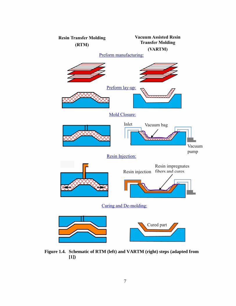
1.1.2.1 The Resin Transfer Molding
RTM is the most traditional LCM process. The steps of the RTM process are
shown on the left hand side of Figure 1.4. First the reinforcements are stacked to form
the desired preform shape. The preform is placed in the mold cavity and the mold is
closed. As the mold is closed and placed in a hydraulic press, the preform takes its
final thickness and it is impregnated with the resin. The resin system is pushed into the
dry preform by the resin injection unit that applies constant pressure or constant flow
rate. After the resin completely wets the dry preform, the injection is closed and the
resin is allowed to cure in the mold. Finally, the cured part in the final shape is
removed from the mold [4].
The main advantages of the RTM process are good surface finish because of
the two-sided rigid mold and high quality final products. The positive pressure from
Page 23
6
the inlet enables the resin to fill the dry preform at higher speeds, which decreases the
cycle time. Since the two-sided mold is kept closed via hydraulic press, mold
deflection can be prevented under high-pressure fillings. By preventing the mold
deflection the dimensional uniformity of the product can be satisfied [5,6]. Also,
higher fiber volume composites can be manufactured with RTM due to higher inlet
forces and rigid and stable mold cavity. The fiber content is described by the fiber
volume fraction, vf; the ratio of the volume of the fibers/preform to the mold cavity.
The mechanical properties of the composite material can be enhanced by increasing
the fiber content [7,8].
The main disadvantage of the RTM is the high initial cost for the mold. This
makes RTM more feasible for small-sized parts with high production rates. For large
and complex part the mold cost might be a deterrent factor. The other disadvantage is
the lack of resin flow monitoring during the impregnation process [9]. If there is a
problem during the impregnation, it cannot be seen until the part is de-molded. This
issue might yield an expensive and inefficient trial and error procedure. However, use
of experimental and simulation tools to design the process can overcome the resin
impregnation issues. Danisman et al. [10] lists a variety of experimental tools
(sensors) to monitor the resin flow and cure cycle in closed RTM mold such as
SMARTweave [11], dielectric [12], ultrasonic [13,14], fiberoptic [15], thermocouple
[9], pressure transducer [16], and point- and lineal-voltage sensors [17,18]. The
simulation tools can also help overcome these issues. Adapting the Finite
Element/Control Volume approach in RTM simulations first implemented by Fracchia
et. al [19] and following simulation tools are developed: RTM-FLOT [20],
PAM-RTM [21], MyRTM [22] and LIMS [23].
Page 24
7
Figure 1.4. Schematic of RTM (left) and VARTM (right) steps (adapted from
[1])
Preform manufacturing:
Vacuum
pump
Vacuum bag Inlet
Cured part
Resin Transfer Molding
(RTM)
Vacuum Assisted Resin
Transfer Molding
(VARTM)
Preform lay-up:
Mold Closure:
Resin Injection:
Curing and De-molding:
Resin impregnates
fibers and cures Resin injection
Page 25
8
1.1.2.2 Vacuum Assisted Resin Transfer Molding
VARTM process is similar to the RTM process except VARTM has one-sided
mold and a nylon transparent layer, vacuum bag, is placed on the other side. As shown
schematically on the right-hand side of Figure 1.4, the process starts with preparing
the preform by placing the layers of reinforcement in the final shape of the product.
The preform is then placed on one-sided mold or a tool surface and the other side is
sealed with a vacuum bag. The sealing between the mold surface and vacuum bag is
achieved with a sealing tape. The vacuum pump, which is placed at the vent, is turned
on to extract the air and creates the pressure gradient to invoke resin flow. The inlet is
closed after the resin wets the preform and reaches the vent. The vacuum is maintained
until the resin cures. Once the resin cures, the part is de-molded.
VARTM process only needs a one-sided mold or a tool surface which reduces
the cost by orders of magnitude and makes it possible to manufacture large structures
such as wind blades. Thus, for large and complex parts VARTM becomes the
manufacturers’ choice [24]. However, VARTM has limitations due to vacuum
pressure. The maximum driving pressure is atmospheric pressure. This limit increases
the fill time and the risk of fill time reaching the gelation time of the thermoset resin
arises, especially for large parts. The fiber content that can be reached with VARTM is
limited compared to RTM as the compaction of the preform is being achieved with
atmospheric pressure [25]. Finally, the surface finish of the vacuum bag side is not as
good as the mold-side.
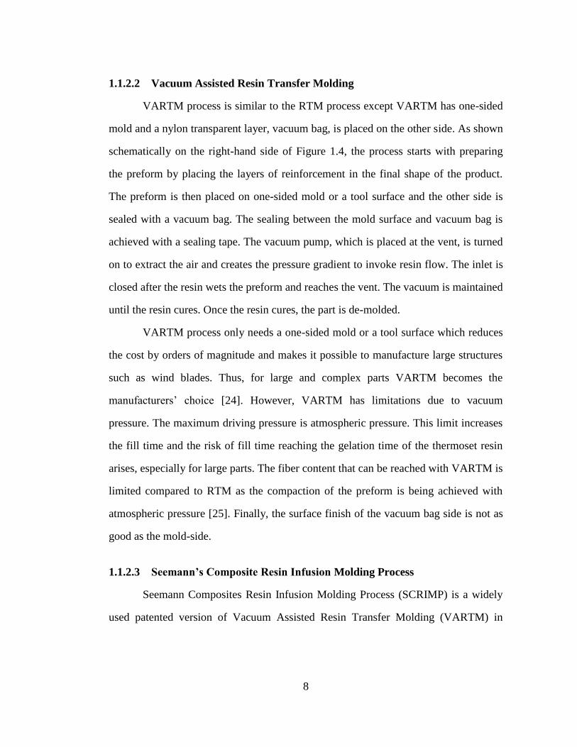
1.1.2.3 Seemann’s Composite Resin Infusion Molding Process
Seemann Composites Resin Infusion Molding Process (SCRIMP) is a widely
used patented version of Vacuum Assisted Resin Transfer Molding (VARTM) in
Page 26
9
which a highly permeable layer (distribution media (DM)) is placed on top of the dry
preform to distribute the resin with very low flow resistance to reduce the filling and
hence the manufacturing cycle time [26]. The schematic in Figure 1.5 shows the steps
of the SCRIMP. As DM is not part of the composite, a peel ply is placed between the
preform and the DM and after the entire assembly cures, peel ply is used to separate
the DM from the composite and discard it.
Figure 1.5. Schematic of SCRIMP steps
Preform manufacturing
Preform lay-up
Mold Closure Resin Injection
Curing and De-molding
Vacuum bag Inlet
Vacuum
pump
Distribution
Media
Distribution
Media (DM)
Resin
impregnates
fibers and cures Resin
injection
Cured part
Peel Ply
Peel Ply
DM
Page 27
10
1.2 Manufacturing Challenges in Vacuum Resin Transfer Molding
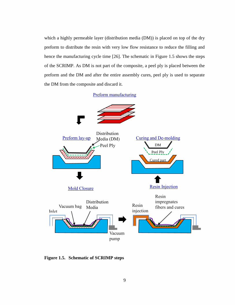
LCM enables tailoring of physical and mechanical properties and creating
complex composite parts. The success of the process depends on the preforming,
impregnation and curing, whereas impregnation is the most challenging part.
Unsuccessful impregnation results in formation of macro- or micro-scale voids.
Macro-scale voids are the large air pockets, dry spots that form due to problems in the
flow front profiles (Figure 1.6.(a)) and micro-scale voids forms around the fiber tows
due to trapped air (Figure 1.6.(b)). Any void that remain in the part after the part cures,
damages the quality of the final part.
Figure 1.6. Examples of (a) macro-void and (b) micro-void [27]
1.2.1 Permeability variation
Flow through porous media with Darcy’s law is used to describe the movement
of resin in the fibrous preform [28]. When using Darcy’s law volume-averaged values
are employed for flow variables such as resin velocity, pressure, and material
(b) Micro-voids
2 4 cm
(a) Macro-voids
0
Dry spot
Trapped air
Page 28
11
properties such as resin viscosity and fiber preform permeability. These averaged
quantities are defined at any location by averaging them over a selected volume
surrounding that region within the domain. However, these fabrics (for example ones
in Figure 1.2) are rarely homogeneous and there can be statistically significant
variation from one region to the next. As shown in Figure 1.7, these variations could
also be due to defects in the fabric. This local non-homogenous architecture of the
fabric can have a noticeable effect on the dynamics of resin flow behavior [29–33].
Figure 1.7. Example of defects in the preform; (a) plain weave glass fabric, (b)
3D orthogonal glass fabric
Most fabrics do have local variations caused by local changes in fiber
orientation and due to change in fabric density [29]. During composite manufacturing
many layers of fabrics are stacked together to build up a certain layer of thickness.
When these layers nest, the nesting may not be uniform across the length of the fabric
may also contribute significantly to permeability variations [30]. Endruweit and
Ermanni [34] found that for a coarse 2x2 twill weave fabric made of thick fiber tows
the variance of local permeability values was higher than for a fine 8-harness satin
(a) (b)
0 1 2 cm 0 0.5 1 cm
Page 29
12
weave fabric for the same fiber volume fraction, which could be explained by the
intrinsic in-homogeneity of the fabric and the relatively high local variations of the
fiber configuration. Quantitative evaluation of injection experiments, which is
normally based on flow front tracking, implies averaging of local variations in
material properties and measuring averaged global permeability values. While the
experimentally determined permeability values characterize quasi-uniform materials,
the accurate predictive description of global flow for non-uniform materials requires
knowledge of the distribution of local properties.
Another challenge during vacuum infusion is the change in the preform
thickness during injection. In RTM resin impregnation is performed through the
preform that is kept between two rigid molds. Assuming the mold design’s stiffness
stands the pressure of the resin and the preform, the preform will not be expanded or
compacted during the filling. However, in VARTM one side of the mold is sealed with
flexible nylon vacuum bag which will not be able to prevent the expansion of the
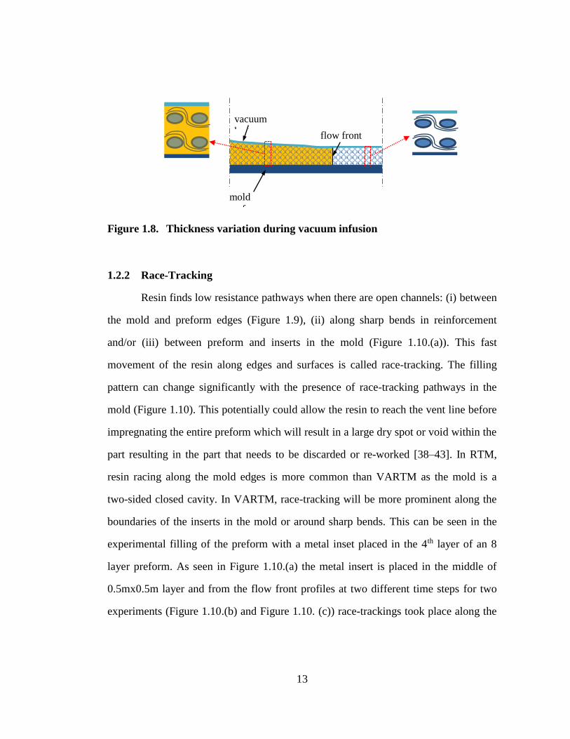
preform during impregnation. As seen in Figure 1.8, the thickness of the preform
changes as the resin propagates [35,36]. This variation arises because of the resin
pressure decreases the compaction. However, this variations does not significantly
affect the resin flow behavior during impregnation [37].
Page 30
13
Figure 1.8. Thickness variation during vacuum infusion
1.2.2 Race-Tracking
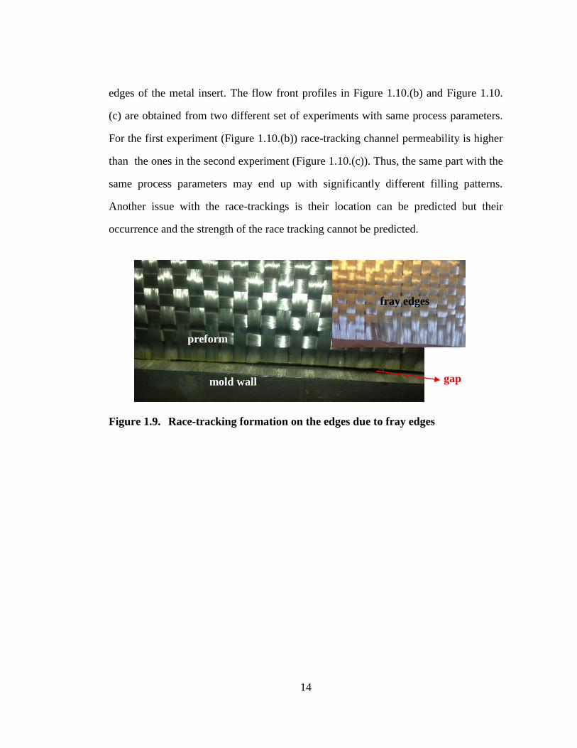
Resin finds low resistance pathways when there are open channels: (i) between
the mold and preform edges (Figure 1.9), (ii) along sharp bends in reinforcement
and/or (iii) between preform and inserts in the mold (Figure 1.10.(a)). This fast
movement of the resin along edges and surfaces is called race-tracking. The filling
pattern can change significantly with the presence of race-tracking pathways in the
mold (Figure 1.10). This potentially could allow the resin to reach the vent line before
impregnating the entire preform which will result in a large dry spot or void within the
part resulting in the part that needs to be discarded or re-worked [38–43]. In RTM,
resin racing along the mold edges is more common than VARTM as the mold is a
two-sided closed cavity. In VARTM, race-tracking will be more prominent along the
boundaries of the inserts in the mold or around sharp bends. This can be seen in the
experimental filling of the preform with a metal inset placed in the 4th layer of an 8
layer preform. As seen in Figure 1.10.(a) the metal insert is placed in the middle of
0.5mx0.5m layer and from the flow front profiles at two different time steps for two
experiments (Figure 1.10.(b) and Figure 1.10. (c)) race-trackings took place along the
mold
surface
vacuum
bag flow front
Page 31
14
edges of the metal insert. The flow front profiles in Figure 1.10.(b) and Figure 1.10.
(c) are obtained from two different set of experiments with same process parameters.
For the first experiment (Figure 1.10.(b)) race-tracking channel permeability is higher
than the ones in the second experiment (Figure 1.10.(c)). Thus, the same part with the
same process parameters may end up with significantly different filling patterns.
Another issue with the race-trackings is their location can be predicted but their
occurrence and the strength of the race tracking cannot be predicted.
Figure 1.9. Race-tracking formation on the edges due to fray edges
preform
mold wall
fray edges
gap
Page 32
15
Figure 1.10. Race-tracking examples: (a) Mid-layer of the preform with metal
insert spatially in the middle, and Flow front profiles at the bottom
of the preform at two different time steps with race-tracking along
the metal insert for two same experimental configurations: (b)
experiment 1, (c) experiment 2
1.3 Modeling of LCM Processes
Modeling the LCM process will allow one to predict the filling pattern, fill
time and the distribution of fluid pressure in the preform. Good understanding of these
issues will allow one to improve the quality and reduce the cost of the composite [44].
Inlet/s and vent/s positions, permeability of the preform, injection rates are the factors
that influence the filling [45]. Numerical simulations have been developed to optimize
processing window and process design to improve manufacturing with LCM [46–51].
In LCM simulations, resin is modelled as a Newtonian fluid that flows in porous
metal insert
inlet line
race-tracking channels
(a) (b)
(c)
Page 33
16
media with averaged pore size. The mathematical description of the resin flow through
porous media that models the physics is Darcy’s law (Equation (1.1)) coupled with
continuity equation (Equation (1.2)), as given below;
⟨𝐯⟩ = −𝐊
µ∇P (1.1)
∇ ∙ ⟨𝐯⟩ = 0 (1.2)
∇ ∙ (−𝐊
µ∇P) = 0 (1.3)
where ⟨𝐯⟩ is the volume averaged resin velocity and P is the pore-averaged resin
pressure, µ is the resin viscosity and 𝐊 is the permeability tensor. The components of
the symmetric, positively definite permeability tensor, K, as shown (in Cartesian
coordinates) in Equation (1.4), represent how easily resin can flow in the
corresponding direction;
𝐊 = [
Kxx Kxy Kxz
Kyx Kyy Kyz
Kzx Kzy Kzz
]. (1.4)
Solution of those equations with the initial pressure and/or flow rate specified
at the inlet gate for the fibrous domain enables the estimation of time to fill the mold,
identification of the optimal locations for placement of gates and vents, and to find
regions which may be susceptible to formation of dry-spots. Fracchia et al. [19],
Bruscheke and Advani [52] and Trochu et al. [53] presented successful 2D resin
impregnation models. Those models are practical for thin parts (for most of the
Page 34
17
composite materials). There are other successful models for both isothermal and
non-isothermal mold filling [49,50,54–61]. As the modeling tools are developed and
improved, those tools are used to optimize the LCM process. If the objective is to have
minimum fill time and/or avoid dry spots, various methodologies have been developed
and reported [4,62,63].
In this dissertation, the numerical simulations of the flow through fibrous
preform are performed via Liquid Injection Molding Simulation (LIMS), which was
developed at the University of Delaware [23]. LIMS is a dedicated finite
element/control volume based simulation of flow through porous media that is capable
of analyzing both 2D and 3D flows. It has both a built in scripted language and a user-
friendly graphical user interface that user can set and perform the simulations. It can
also be called from Matlab® as a function to be used for optimization routines. As
represented in Figure 1.11, the program requires the mesh geometry, viscosity of the
resin, permeability tensor, porosity/fiber volume fraction with boundary conditions
and it provides the flow front locations with time, the last region to fill and the fill
time along with pressure distribution and the success of the filling (location of dry
spots, if any). The permeability values of the reinforcements are relatively low, so the
resin flow is slow (low Re, Re<10). Therefore LIMS adopts the quasi-steady state
assumption. At each step the pressure distribution is obtained from Darcy’s Law
(Equation 1.1) and the Continuity Equation (Equation 1.2). From the pressure
distribution the flow front is advanced using the Darcy’s Law (Equation 1.1) for resin
velocity. Hence one can design gate and vent locations if the preform permeability
map and the permeability tensor in the preform domain (Figure 1.12), are known with
certainty and do not change from one part to the next.
Page 35
18
Figure 1.11. Liquid Injection Molding Simulation (LIMS) Structure
Figure 1.12. Permeability map approach
K1
K2
K3 K
4
K5
K6
K7
K8
K9
K10
K11
Page 36
19
1.4 Objective and Dissertation Outline
Research objective of this dissertation is to develop a methodology to create a
spatial distribution of the permeability tensor, called the permeability map for a given
geometry (Figure 1.12), that will allow the mold cavity to fill from a gate and arrive
last at the vent (which implies no voids) despite variability in the preform and flow
disturbances around the mold walls, inserts and corners. The simulation output is the
void area where the input is the geometry of the part along with the permeability map,
location and strength of flow disturbances, location of gates and vents and the inlet
pressure or flow rate boundary condition at the gates. The goal is to find a
permeability map for a selected gate and vent location that will give at most a small
void region despite flow disturbances and variability in preform permeability.
In order to achieve this objective one needs; (i) to develop a characterization
method for permeability, (ii) to be able to quantify the variability in the fabric due to
manufacturing variability of textiles, (iii) to identify race-tracking and other issues of
the fabric and their effect on permeability, replaced by, (iv) to develop optimization
methods that create permeability maps despite variations to achieve successful filling.
In this dissertation, after the introduction to LCM processes in Chapter 1,
permeability measurement and characterization methods are presented in Chapter 2.
Also, a methodology is introduced to characterize the six components of the
permeability tensor with non-zero skew components.
In Chapter 3, the 3D permeability characterization technique introduced in
Chapter 2 is used to demonstrate that slight variation in orientation during lay-up can
influence through thickness permeability variability dramatically and a permeability
map should take this into consideration.
Page 37
20
Chapter 4 introduces a technique to quantify variation in permeability of a
fabric which will be taken into account when assigning a permeability map
Chapter 5 presents the formulation of a methodology and development of
optimization technique that will use the forward simulation allowing for variability in
permeability to create a permeability map that will fill the mold without voids despite
the variations and flow disturbances.
The last chapter lists the conclusions and contributions with suggestions for
future work.
Page 38
21
Chapter 2
PERMEABILITY MEASUREMENT TECHINIQUES
2.1 Historical Background
In 1856 Darcy conducted sets of water flow through sand beds experiments
which was the first attempt to model fluid flow through porous domain [64]. He
introduced the term permeability to quantify the ease of fluid flow in porous domain
and developed an empirical relationship to relate the flow rate of water to the pressure
drop across the sand column as follows
Q = −KA
µ∙
∂P
∂x (2.1)
where Q is the flow rate, µ viscosity of water, A is the cross-sectional area, ∂P
∂x is the
pressure gradient along the flow direction and K is the scalar that characterizes the
permeability of the sand in the flow direction.
Darcy developed the equation for homogeneous and isotropic porous domain
with water flow in one-direction. In 1961 Liakopoulos [65,66] expanded the Darcy’s
empirical equation by introducing the permeability as a tensor. The permeability
tensor (Equation 1.4) characterizes the ease of resin flow in porous domain in all
three-directions.
Symmetric, positively definite permeability tensor, K has orthogonal set of
axes – principle directions (which are the diagonal terms when the non-diagonal terms
are zero). Figure 2.1 shows the mold coordinate (xyz) and the principle direction of
Page 39
22
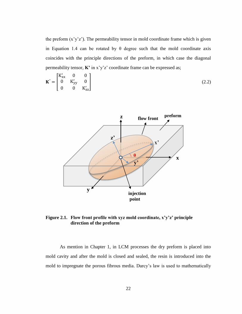
the preform (x’y’z’). The permeability tensor in mold coordinate frame which is given
in Equation 1.4 can be rotated by θ degree such that the mold coordinate axis
coincides with the principle directions of the preform, in which case the diagonal
permeability tensor, K’ in x’y’z’ coordinate frame can be expressed as;
𝐊′ = [
Kxx′ 0 00 Kyy
′ 0
0 0 Kzz′
] (2.2)
Figure 2.1. Flow front profile with xyz mold coordinate, x’y’z’ principle
direction of the preform
As mention in Chapter 1, in LCM processes the dry preform is placed into
mold cavity and after the mold is closed and sealed, the resin is introduced into the
mold to impregnate the porous fibrous media. Darcy’s law is used to mathematically
preform
injection
point
z flow front
x’
y’
z’
θ x
y
Page 40
23
describe the flow of resin into a closed mold containing fiber preform. However, how
closely the mathematical model mimics the actual flow behavior depends on the
fidelity of the material input data such as viscosity of the resin and the permeability
values of the fabric placed in the mold. Hence it is important to characterize the
permeability data accurately. Over the years, researchers have presented many
different methodologies to characterize the permeability of the fabric. The overall
approach to permeability characterization can be investigated under three broad
categories (i) analytical and predictive methods, (ii) numerical methods and (iii)
experimental methods.
2.2 Analytical and Predictive Methods
As a mathematical model, Darcy’s Law, relates the pore-averaged velocity
with the pore-averaged pressure gradient with the permeability of the porous domain,
K and the viscosity of the resin, µ (Equation (1.1)). Darcy’s Law is a macroscopic
model and the microscopic physical properties are averaged using continuum
approach. Thus, the effect of the fiber volume fraction (namely porosity), tortuosity
and capillary effects are lumped under permeability in Darcy’ Law [67].
Kozeny-Carman (KC) tried to establish a relationship between permeability
and porosity by modeling the flow within a porous media as a series of cylinder
capillary channels coupled with Carman’s introduction of hydraulic channel [68]. The
Kozeny-Carman equation can be expressed as;
K = 𝑅𝑓
2
4𝑘0
(1 − 𝑣𝑓)3
𝑣𝑓2 (2.3)
with 𝑅𝑓 is the fiber radius, 𝑘0 is the Kozeny constant that empirically accounts for the
tortuosity to be determined experimentally and 𝑣𝑓 is fiber volume fraction.
Page 41
24
KC equation is a semi-empirical relation with 𝑘0 empirical constant which is
later proved not to be constant [69]. The KC model improvements are performed to
estimate the permeability [70]. Ahn et al. [71] showed good agreement in permeability
estimation for woven fabrics using KC, however, Gauvin et al [72] reported KC model
is not sufficient for random mats. Also, unsuccessful experimental implementations
are presented [73]. Thus, researchers suggest the introduction of the capillary model
for the resin flow to improve the estimations.
Gebart [74] developed a geometric model for permeability prediction. Set of
analytical expressions are presented for an idealized unidirectional reinforcement with
regular, parallel fibers. The expressions consists of Navier-Stokes equations both for
flow along and perpendicular to the fibers. Solution for the flow along the fibers has
the same form with KC formulation, however, for perpendicular flow includes the
physical limit in terms of fiber volume fraction. Another predictive model is
introduced by Bruschke [75]. The model consists of regular array of cylinders to
represent the fiber tows. Close form solutions are derived for the upper and lower fiber
volume fraction values for Newtonian fluids. Good agreement is obtained between
closed form solutions and numerical models for mid-range fiber volume fractions. The
limitation of Gebart and Bruschke models is that the physical model used to describe
the system does not capture the structural details of real preform materials. The fiber
preform usually used in LCM processes consist of woven or stitched fiber bundles
known as tows or yarns, rather than of individual fibers and their geometric
arrangements are usually more complex than the one assumed in analytic models.
Since, predictive tools cannot represent the realistic geometrical arrangement,
Page 42
25
experimental and numerical methods are more useful for permeability
characterization.
2.3 Numerical Methods
Numerical methods, as a tool to characterize the permeability, generally
involves the solution of the Navier-Stokes equation for well-defined cell geometry for
the preform. The solution involves either use of periodic boundary conditions or
implementation of the Lattice-Boltzmann method. All methods impose a pressure
drop across the porous domain and calculate the average flow through the unit cell or
prescribe a flow rate along one face of the unit cell and calculate the pressure drop.
The permeability of the unit cell is derived by using the Darcy’s Law.
Averaging of permeability in a unit cell is an example of homogenization
method. Over the macro-scale, the equivalent homogeneous medium represents the
average behavior of the heterogeneous medium. Mathematical theory of the
homogenization method is established in several studies [76]. The numerical method
solves the Navier-Stokes equation for the homogeneous medium, representative unit
cell using the periodicity boundary condition [77].
The Lattice-Boltzmann Method (LBM) is based on microscopic models and
mesoscopic kinetic equations. The methods models the fluid as set of particles that are
moving and interacting on a lattice. From the discrete data of the particles, one can
define the space and time aspects of the fluid flow.
LBM has been used to investigate the porous media by several authors [78–
81]. Koponen et al. [78] employed the nineteen velocity LB model to calculate
permeability of three dimensional random fibrous structure generated by a growth
algorithm in discretized space. Nabovati and Sousa [82] investigated the permeability
Page 43
26
of sphere packs. Also Nabovati and Sousa [82] reported their work on fluid flow in
three-dimensional random fibrous media simulated using the lattice Boltzmann
method.
The LBM overcomes the major limitation of the homogenization method. It is
capable of simulating flow in realistic situations of complex fabric geometries and
structure. However, Belov et al. [83]reported that the Lattice Boltzmann calculations
are computationally intensive. But it can also incorporate the surface tension effects of
the fluid very easily.
The numerical solutions providing permeability data for the unit cell, may not
accurately represent the permeability of the preform at the macro-scale. To perform an
entire simulation within a preform with thousands of unit cells solving for Navier-
Stokes equation may be a formidable computational challenge. Hence, experimental
methods are used to determine the permeability coupled with phenomenological and
numerical methods since the permeability changes with fiber orientation and fiber
volume fraction; otherwise one would have to conduct many experiments for the same
fabric to find the dependence on fiber orientation and volume fraction.
2.4 Experimental Measurement Techniques
Permeability characterization experiments are performed by controlling either
inlet pressure or injection flow rate and grouped according to the pattern of fluid flow
through the preform: rectilinear, radial, transverse and three-dimensional. Each
approach has its own advantages and disadvantages.
Page 44
27
2.4.1 Rectilinear Flow
In-plane permeability measurements are the most commonly reported in
literature as they are straight forward. Rectilinear experimentation is an in-plane
permeability measurement technique to characterize the permeability by conducting
linear flow channel experiments [84–86]. The preform can be placed either in a RTM
mold with one transparent side or a VARTM set-up. As the resin flows through the
preform, linear flow front profiles are tracked with time, as shown in Figure 2.2. For
an ideal experimentation, the flow front profiles will be linear and can be easily
monitored. The experimental data is the flow front position with time. Then, time
integration of one-dimensional Darcy’s Law yields the solution of the flow front
position with time, as given in Figure 2.2. In this equation, xf(t) is the flow front
position at time t, K is the permeability of the preform in the flow direction, ΔP is the
resin pressure drop along the flow, μ is the resin viscosity and 𝜙 is the preform
porosity (defined as (1-vf)). From the slope of the best line fit of the plot of the square
of the experimental flow front, the average bulk permeability of the fabric in the flow
direction can be evaluated for that particular fiber volume fraction.
Page 45
28
Figure 2.2. One-dimensional permeability characterization experiment to find
the bulk permeability value in the direction of flow
Rectilinear flow experiment is easy to conduct and the experimental data is
easy to process and have high reproducibility [84,87,88]. However, appropriate
equipment, such as visualization tools and sensors, might increase the initial cost
which can be listed as a disadvantage. Another disadvantage arises due to the
race-tracking issue (as introduced in Chapter 1) which invalidates the linear flow
assumption and generates error in permeability data [42,89]. As mentioned before,
this approach is used to determine the permeability component only in the flow
direction. Set of experiments are required for characterization of all the six
components of the permeability tensor.
Preform Filled region
𝑥𝑓(𝑡): flow front location at time 𝑡
Linear flow fronts
used to find bulk
permeability
Actual flow fronts 𝑡1
𝑡2
𝑡3
Page 46
29
2.4.2 Radial Flow
Radial flow is another method for in-plane permeability characterization. The
test fluid is injected through a gate which is a hole in the center of the fiber preform.
The resin entering in the circular cutout in the middle of the preform spreads radially
impregnating the preform in a circular or elliptical shape. The radius of this boundary
is important during the data analysis. As seen in Figure 2.3, if the preform is isotropic
the flow front profiles are circular and as the anisotropy of the preform increases the
major minor axes ratios increases. The ellipses’ major and minor axes align with the
principle direction of the preform and the ellipse is at an angle with respect to global
coordinate frame if the principal axis of the preform do not coincide with the
coordinate axis (as shown in Figure 2.3.(c)).
Radial injection eliminates many of the disadvantages of the rectilinear flow
[85,90–97]. However, flow front tracking requires visual monitoring through the
transparent mold surfaces [98,99], fiber optic sensors [71], thermistors [100], pressure
transducers [101], and ultrasound and electrical residence [102]. Then, data reduction
schemes are required. Additionally data reduction schemes is more complex than the
linear flow experimental data. Though, for isotropic preforms the analytical solution of
the in-plane permeability can be calculated easily [103];
K = {𝑅𝑓2[2 ln(𝑅𝑓 𝑅0⁄ ) − 1] + 𝑅0
2} 1
𝑡
𝜇𝜙
4Δ𝑃 (2.4)
where 𝑅𝑓 is the flow front radius at time t, and 𝑅0 is the radius of the injection gate.
Thus, using equation 2.4, permeability of isotropic preforms can be determined by
measuring the pressure gradient and monitoring the circular flow fronts with time.
Then, for the anisotropic fabrics Chan and Hwang [91] proposed an approach to
determine the principle permeability components using the major and minor radius of
Page 47
30
elliptical flow front profiles (Figure 2.3.(b)). This work is followed by Weitzenbock et
al. [103,104] with the methodology to obtain the principle permeability components
without the knowledge of the principle axes (Figure 2.3.(c)).
Radial flow experimentation can be used to characterize in-plane permeability
components. Moreover, the race-tracking issue doesn’t occur in radial injection and
doesn’t affect the permeability evaluation. However, radial flow experiments are
consistent with linear flow but result in different values for the same preform at the
same fiber volume fraction. However, for a reliable in-plane permeability data Wang
et al. [85] suggests conducting both linear and radial flow experiments.
Page 48
31
Figure 2.3. Schematic of radial flow front profiles: (a) isotropic (R1=R2), (b)
anisotropic (R1≠R2), (c) anisotropic with non-zero in-plane skew
term (global coordinate frame doesn’t coincides with principle
directions of the preform)
(a) Isotropic flow front
(b) Anisotropic flow front
(c) Anisotropic flow front
with non-zero
in-plane skew term
Injection point, R0
R1 R
2
R1
R2
θ
R2
R1
Preform
x
y
Page 49
32
2.4.3 Transverse and Three-Dimensional Flow
A variety of methods that have been used to experimentally characterize the
in-plane preform permeability components are presented in the previous section. For
thin parts only in-plane permeability is required which has three independent
components – either two principal values and the orientation of principal axes or two
normal and one “skew” component. For thick parts, one must characterize through the
thickness permeability as well [95,100,105–107].
There are two approaches for transverse permeability measurement;
simultaneous measurement of three principle permeability components and
independent measurements (separate experimentations for in-plane and transverse).
Several researchers conducted transverse permeability studies [100,108–110].
One-dimensional channel flow apparatus is utilized to characterize this component
with Darcy’s Law [111].
Trevino et al. [112] developed a tool to evaluate the transverse permeability
based on one-dimensional flow and discretized Darcy’s Law. Wu et al. [113] includes
the three-dimensional flow simulation to one-dimensional flow model using steady
state flow profiles. Ahn et al. [71] presents a device that simultaneously measures the
transverse permeability and capillary pressure.
In order to model the three-dimensional resin impregnation, three-dimensional
permeability characterization is required. Three-dimensional flow experiments are
proposed to fully characterize both isotropic and anisotropic permeability with a single
experiment. Traditionally, LCM parts are thin but there are practical resin flow
problems seeking for three-dimensional permeability tensor [100].
A general methodology is presented by Woerdeman [110] for
three-dimensional permeability tensor characterization from set of one-dimensional
Page 50
33
flow experiments. The permeability data is derived from numerical solution of six
nonlinear equations [114]. Whereas, Weitzenbock et al. [100] tracked the flow fronts
using thermistors and mentioned the importance of the capillary pressure on the
three-dimensional permeability characterization. Using the same measurement
principle Ahn et al. [71]monitored the flow fronts using embedded fiber optic sensors
which are placed inside the preform. Following that, Ballata et al. developed Smart
Weave as another flow monitoring technique [115].
Gokce et al. [116] introduced a new experimental method, Permeability
Estimation Algorithm (PEA). PEA processes flow front information during the
experimentation and process with a numerical process model. Its limitation is being
applicable only for VARTM process. Whereas, Breard et al. [117] used X-ray
radiography to monitor the flow but the cost of the system requires expensive tooling.
Nedanov et al. [114] presents a method to evaluate principle values of the
three-dimensional permeability tensor. This method is based on visual monitoring of
the in-plane flow front profiles. The shape and size of the in-plane flow front through
the transparent membrane as well as the amount of fluid in the preform and elapsed
time are recorded and allow for characterization of principle permeability in all three
directions. Similar approach is used by Okonkwo et al. [118]. Instead of transparent
plates, electrostatic sensors are placed on the top and bottom surfaces of 3-D radial
injection mold is used and instead of an analytic solution, numerical simulation is
utilized to characterize the permeability.
Each of these experiment approaches has their disadvantages. The use of
embedded sensors affects the pattern of flow and renders the experimental data
unreliable. Weizenbock [100] observed that the flow front in the part of the mold
Page 51
34
where the thermistors sensors had been placed was lagging behind compared with
other undisturbed parts of the mold. Also since the sensors are normally embedded in
the preform manually, this requires time and effort. Numerous experiments are usually
required for reliable characterization of preform permeability and as such using
embedded sensors will require extensive time and labor rendering the methods less
efficient. And the method [117] that involves the use of X-ray spectroscopy to
measure the flow front through the thickness is rather expensive. In case of Nedanov
experiments [114], the results for through thickness could be unreliable as they used
only one data point to find the transverse permeability –which was when the arrival of
the resin was recorded at the bottom. Also the size of the gate had an effect on the
permeability calculations. The method developed by Okonkwo et al. [118] is
applicable to non-conductive fabrics, e.g. cannot be implemented to carbon fibers.
From the review of the existing experimental methods for permeability
characterization of fibrous media shows that while traditional methods for in-plane
permeability measurement are well developed the methods for transverse permeability
measurement need further investigation. Hence the need for reliable and fast method
to determine the components of the three-dimensional permeability tensor in a single
experiment and use of simple equipment is desirable.
2.5 Skew terms
For thin parts, only in-plane permeability (Kxx, Kxy, Kyy) are necessary. That
requires three components – either two principal values and the orientation of
principal axes or two normal and one “skew” component (Kxy). Several methods to
obtain these values were devised. For thick parts, particularly when flow media is used
Page 52
35
on part surface, through the thickness permeability is needed as well and can be
measured [119–122].
Three-dimensional tensor contains not only this (normal) transverse
permeability but also two additional skew components. These are, in practice,
neglected as it is assumed that fabric layering produces symmetry needed to eliminate
them. This assumption is somewhat questionable in the first place, but it becomes truly
invalid when thick, three-dimensionally woven or braided reinforcements are
concerned. The geometry of weave allows these terms to appear and acquire some
significance for flow. So far, no methods have been developed to measure these terms
for thick preforms and it remains uncertain how important they are for the
manufacturing process. In this section, permeability tensor is investigated for thick
3-D woven fabrics, including the skew components via a multi-objective optimization
algorithm coupled with Liquid Injection Molding Simulation (LIMS) tool. The effect
of the skew components on the resin impregnation and the limitations on the
importance of those terms are evaluated.
2.5.1 Introduction
Three-dimensional fabric permeability tensor requires in addition to the
transverse permeability, two additional out of plane skew components if the through
thickness principal direction is not orthogonal to the plane of the fabric. Most
researchers assume that the principal Kzz direction of the fabric coincides with the
z-axis. This assumption may not be true for thick, three-dimensionally woven or
braided textile fabrics as the ones shown in Figure 2.4. The geometry of the weave
could be such that the principal Kzz direction may not be aligned with the normal
direction of the preform plane. This will influence the resin flow pattern in a mold due
Page 53
36
to the non-zero skew components (Kxz and Kyz not being equal to zero). So far, no
methods have been developed to measure these terms for thick, unbalanced and
braided preforms and it remains uncertain how important they are for the
manufacturing process.
Figure 2.4. 3D 25890 g/m3 E-glass fabric
In this chapter a methodology is presented to determine these skew terms using
radial flow experiments in an instrumented mold. Flow front profiles at the top and the
bottom of the mold are used to construct the flow front pattern at the top and bottom of
the preform respectively. Using a multi-objective optimization algorithm, the input
values for the permeability tensor in the flow simulation program LIMS are varied
until the flow front patterns at the top and the bottom of the mold in the simulation
match with the experimental results.
Page 54
37
2.5.2 Methodology
To characterize the permeability, the fibrous preform is placed in the mold,
which consists of transparent acrylic top and bottom surfaces connected via aluminum
spacers and steel bolts. A resin injection hose is connected to the center of the bottom
surface, and the resin is contained in a pressurized vessel. Two video cameras are
placed and synchronized so as to capture images of the top and bottom surfaces of the
mold simultaneously. The recorded images contain a timestamp in their file name.
After recording the fiber volume fraction and viscosity, the resin is introduced into the
mold under constant pressure from the pressurized tank. The experiment is recorded
until the flow front reaches any edge of the mold. The experiment set-up is given in
Figure 2.5.
The fill times and flow front characteristics are determined experimentally via
image-processing, an example of which is shown in Figure 2.6. The images captured
during the experiment are input into a MATLAB® script, which processes and
analyzes them. The images are filtered and converted to binary, so that it only contains
a white elliptical ring, which represents the progress of resin flow from the preceding
image to the current one. The script iterates through each image to record the locations
of pixels in the flow front. These pixel locations are provided as input to a MATLAB
function that generates an ellipse for the flow front using a least squares fit method.
Given a set of ideal images (distinct resin flow edges with no noise) taken from a
virtual experiment so that the actual fill times were known, the approximated fill times
from image processing were shown to have an average relative error of less than 2.0%.
From the fitted ellipses, the script can also determine characteristics such as; the semi-
major and minor diameters, the angle of rotation, and centroid location.
Page 55
38
Figure 2.5. Experimental set-up to monitor the resin flow at the top and bottom
surfaces of the preform (left: schematic, right: picture of the set-up)
The permeability tensor is evaluated by minimizing the difference between the
experimental flow-fronts and the flow-fronts numerically predicted with six
permeability components as variable parameters. The minimization uses Nelder-Mead
simplex method. This method is designed to solve unconstrained multi-objective
minimization/maximization problems. The method needs initial function values to
form the initial simplex but does not require any gradient input. The method is a
simplex-based method where a simplex, S, in n-space is defined as a convex hull of
n+1 vertices. For example, a simplex in a 2D space is a triangle and in a 3-D space is a
tetrahedron. The method begins with n+1 points (vertices of initial simplex) and
function values at those points for n-variable optimization. The method then performs
a sequence of transformations of the working simplex, S, aimed at decreasing the
function values at its vertices. At each step, the transformation is determined by
Page 56
39
computing one or more test points, together with their function values, and by
comparison of these function values with those at the vertices. This process is
terminated when the working simplex, S, becomes sufficiently small that satisfies the
assigned tolerance. For this study the generation of the new simplex algorithm is
adopted from Mathews and Fink [17].
Figure 2.6. (Left) An image of isotropic flow from an experiment. (Middle) The
image after having the preceding flow image subtracted from it,
filtered, and converted to binary. (Right) An ellipse is fitted to the
edge of the resin flow front.
In this optimization routine the objective function is to minimize the residual
sum of square of the experimental and numerical fill times of the filled nodes located
at the top and bottom surface of the mold (Figure 2.7). The flow with initial
permeability values is simulated via a numerical tool called Liquid Injection Molding
Simulation, LIMS, which is a finite element/control volume based program that uses
Darcy’s law to describe the flow of resin inside a fibrous media and tracks the flow
front during the impregnation process [45] with input values provided for the
permeability and viscosity. LIMS then outputs the calculated node fill times, and the
-0.1 -0.05 0 0.05 0.1 0.15
-0.1
-0.05
0
0.05
0.1
0.15
x
y
a (x2)+b x y+c (y2)+d x+e y+f = 0
Page 57
40
computation is made to converge using the Residual Sum of Squares (RSS) method
with the difference between the experimental fill times and the simulated fill times.
This process is iterated by updating the input values for permeability until the LIMS
fill times are sufficiently close to the experimental fill times. Those final input
permeability values in LIMS are the permeability values for the fabric
One of the main advantages of this method to characterize the permeability
tensor is that it is inexpensive and easy to implement. Okonkwo et al. [118] proposed
a similar algorithm, however the experiment involved a heavy mold with an expensive
set of electric resistance sensors. The use of electric resistance sensors excludes the
use of carbon fiber preforms, as carbon fiber is electrically conductive. The method
described in this paper requires no sensors, as it uses image-processing as its primary
means of calculating fill times. Also, the mold is relatively light and simple to set up
and clean, while a senor-based experiment would require a more tedious clean-up
process; if the resin is not completely cleaned off of the sensors, it could obstruct the
sensors and the subsequent experiment could yield unreliable data. Other proposed
methods have used embedded optical fiber sensors, which obstruct resin flow, leading
to inaccurate data. Another benefit of this method is that K can be characterized in a
single radial flow experiment, and the top and bottom surfaces of the mold are
accounted for so as to allow one to determine all the six independent components of
the three-dimensional permeability tensor. Weitzenböck et al. [93] proposed a method
for measuring the permeability components in one radial flow experiment, however
the resin was to be injected uniformly in the through-thickness direction. Therefore
only in-plane components of K could be determined.
Page 58
41
Figure 2.7. Algorithm for permeability prediction from experimental fill time of
top and bottom surfaces
2.5.3 Results and Discussion
First, the methodology is tested with a parametric study of radial injection from
the bottom center of the mold cavity injected under constant pressure. Figure 2.8
demonstrated the effect of non-zero skew terms; Kxy, Kxz and Kyz on the flow pattern.
In Figure 6.a-c the magnitude of Kxy is increased while other two skew terms are zero
to investigate its influence on the flow front. As expected increase in-plane skewness,
Kxy, yields an increase in the in-plane rotation of the elliptical flow fronts. The center
of the ellipses observed along the top and the bottom surfaces coincide and do not shift
with the magnitude of Kxy. Nor do the ratios of the major and minor axes change,
only the angle of the in-planar rotation increases with increasing Kxy. However, as the
Page 59
42
other two skew terms, Kxz and Kyz are assigned a non-zero value, the center of the top
ellipse in no longer coincident with the ellipse at the bottom surface. The shift between
the two centers is proportional to the magnitude of the skew terms. As the Kxz value is
increased the distance between the centers of the ellipse on the top surface and the
bottom surface increases along the x-direction (Figure 2.8.d-f), similarly as the Kyz
value is increased, the distance between the top and the bottom center increases in the
y-direction (Figure 2.8.g-i). The numerical approach presented in Figure 2.7 is applied
to the ellipses of Figure 2.8 in order to predict the permeability tensor just using the
top and bottom ellipse flow front information. The maximum error between the
assigned permeability and the predicted one is found to be 3.33 %
Furthermore, the methodology is validated by assigning six non-zero
permeability components in the LIMS simulation. The flow fronts on the top and
bottom surface of this virtual experiment are used in the approach presented in Figure
2.9, to find the six components of the permeability tensor based on just this
information as follows; the permeability tensor values on the left side in Table 2.1 are
assigned into LIMS and resin arrival time are obtained with the developed image
processing tool from the images of the top and bottom at different time steps. These
arrival times are used as the experimental fill time (Ti,exp in Figure 2.7). Also, from the
flow front profiles at the top and bottom the ratios of the in-plane permeability
components and the angle between the principal directions and the global coordinate
frame can be estimated. These estimations are assigned as the initial simplex. The
algorithm converged to the assigned permeability values listed on the right side of
Table 1 in about 6 hours of CPU time on a PC computer. In Figure 2.9, the flow front
profiles are compared with the assigned and predicted permeability values for the top
Page 60
43
and bottom surfaces. At time equal to 90 seconds the resin reaches the top for the first
time and as it impregnates the top surface to form the ellipse, the center of the top
ellipse is not coincident with the center of the ellipse at the bottom because of the
non-zero Kxz and Kyz. This virtual experiment also shows the methodology can predict
the six components of the permeability tensor accurately.
Next, the methodology is applied to characterize the 3D glass fabric with 2627
g/m2 areal weight. Three layers of 3D fabric are placed in the mold cavity with
dimensions of 25.4 cm x 25.4 cm x 0.6 mm with 60% fiber volume fraction. Due to
Newtonian behavior, colored corn syrup diluted with water with viscosity of 107 cP is
used as simulated resin. The images with time stamps are analyzed via the image
processing routine and the fill times at the bottom and top nodes are derived as the
experimental data. Then the algorithm given in Figure 2.7 is implemented. Table 2.2
shows the results of predicted permeability components. From the predicted
permeabilities, the Kxz component is seen to be negligibly small, but Kyz values is
found to have effect on resin impregnation.
In Figure 2.10, experimental flow front profiles are compared with the profiles
obtained using the predicted permeability values provided in Table 2.2 at time equal to
13.26 seconds. As it can be seen in the figure, the match between experimental and
predicted profiles is quite good. The major and minor axes values are compared are
also compared. For the top, experimental major and minor radius are 0.055 m and
0.028 m and the prediction data are 0.050 m (9.09% error) and 0.029 m (3.57% error),
respectively. For the bottom, experimental major and minor radius are 0.086 m and
0.051 m and the prediction data are 0.085 m (1.16% error) and 0.052 m (1.96% error),
respectively.
Page 61
44
Figure 2.8. Flow front profiles at the top (solid lines) and bottom (dash-dot lines)
for different skew permeability at time equal to 700 seconds. The
jagged flow fronts are numerical artifacts because of fairly coarse
mesh.
Kxz = Kyz = 0
Kxy
= Kyz
= 0
Kxy
= Kxz
= 0
(a) Kxy
= 1.0x10⁻¹¹ (b) K
xy =3.0x10
-11 (c) K
xy = 7.0x10
-11
(d) Kxz
= 1.0x10⁻¹²
(e) Kxz
= 3.0x10⁻¹²
(f) Kxz
= 7.0x10⁻¹²
(g) Kyz
= 1.0x10⁻¹²
(h) Kyz
= 3.0x10⁻¹²
(i) Kyz
= 7.0x10⁻¹²
*For all simulations: Kxx
= 2.0x10⁻¹⁰
Kyy
= 1.0x10⁻¹⁰
Kzz
= 1.0x10⁻¹²
δx δx δ
x
δy δ
y δ
y
x
y
Page 62
45
Table 2.1. Parameters for virtual experiment
Parameter: Numerical value:
Inlet pressure: 1.0 bar
Fiber volume fraction of E-glass: 50%
Viscosity of corn syrup 100 cP
Assigned
Permeability (m2)
Predicted
Permeability (m2)
Percentage
Error (%)
Kxx 2.0x10⁻¹⁰ 1.979x10⁻¹⁰ 1.05
Kxy 1.0x10⁻¹¹ 9.895x10⁻¹² 1.05
Kyy 1.0x10⁻¹⁰ 9.884x10⁻¹¹ 1.16
Kxz 5.0x10⁻¹² 4.947x10⁻¹² 1.06
Kyz 2.5x10⁻¹² 3.875x10⁻¹² 3.12
Kzz 1.0x10⁻¹² 9.798x10⁻¹³ 2.02
Figure 2.9. Flow front profiles comparisons with assigned and predicted
permeability values at the top and bottom surfaces
x
y
Top Bottom Assigned
Predicted
Level Time(sec)
1 300
2 400
3 500
4 600
5 700
δ
Page 63
46
Table 2.2. Predicted permeability for the experiment
Kxx Kxy Kyy Kxz Kyz Kzz
2.405x10⁻¹¹ 7.451x10⁻¹² 1.736x10⁻¹⁰ 5.777x10⁻¹⁶ 7.365x10⁻¹³ 1.911x10⁻¹²
Figure 2.10. Flow front profiles at time 13.26 seconds at the top and bottom:
experimental, with predicted permeability and comparison
-0.1 -0.05 0 0.05 0.1
-0.1
-0.05
0
0.05
0.1
x
y
a (x2)+b x y+c (y2)+d x+e y+f = 0
Experimental With predicted permeability Comparison
TOP
BOTTOM
Experimental With predicted permeability Comparison
Page 64
47
2.5.4 Summary
This work presents a methodology to characterize all the six independent
components of a three dimensional second order permeability tensor. The approach
employs a multi-objective optimization algorithm coupled with Liquid Injection
Molding Simulation (LIMS) tool to calculate the permeability values. The effect of the
non-zero skew components on the flow front progression and flow patterns is
investigated through a virtual study to underline when the skew terms could change
the nature of filling and influence the manufacturing process.
Page 65
48
Chapter 3
THROUGH THICKNESS PERMEABILITY
3.1 Introduction
When unidirectional stitched fabrics are used as reinforcement in composites,
plies are typically stacked on top of each other to build up the desired thickness.
Strength and stiffness requirements dictate the orientation of individual layers and the
accuracy of angular alignment is limited. A pressure differential across the thickness is
used to distribute the resin, either from a pre-impregnated fabric or injected from a
resin source, to occupy all of the empty spaces between the fibers. This process is
commonly modeled using Darcy’s law, which describes flow of resin through porous
media in which the flow rate is directly proportional to the applied pressure
differential by the through-thickness permeability of the fabric. A different orientation
between layers or even a slight misalignment during the stacking can change the
through-thickness permeability dramatically due the change of resin pathways. In this
chapter, characterization of the through-thickness permeability of a series of
unidirectional fabrics stacked in various orientations is studied to address both the
effect of stacking sequence and those of misalignment of the individual layers.
Numerical simulations are conducted to predict the effect of change in fiber
orientation on the through-thickness permeability. The results from the numerical
model are compared with experimental measurements. Results show that averaging
approach is not suitable to calculate the through-thickness permeability component
when using unidirectional fabrics and that the stacking sequence of the unidirectional
Page 66
49
fabrics may significantly influence the through-thickness permeability. Also, it has
been shown that the effects of misalignments smaller than 5 degrees rotation between
individual layers do not significantly modify the transverse flow.
This chapter will analyze through-the thickness flow depending on relative
orientation of individual reinforcement layers. It will show that such an averaging
approach can result in large errors in calculation of the through-thickness permeability
component when the preform consists of layers of unidirectional fabrics stacked in
different desired fiber orientations. It will be shown both experimentally and by
modeling, that the stacking sequence can significantly influence the through-thickness
flow and hence the transverse permeability. This study will show that a limited
misalignment less than 5 degrees rotation between the neighboring layers – which can
be attributed to inaccuracy of the layup process – does not significantly modify the
through the thickness permeability.
A numerical study for a simplified model fabric is shown in Figure 3.1.
Through-the-thickness direction is aligned with the z-axis. It is assumed that this is the
principal direction of permeability and hence Kyz and Kxz are assumed to be zero. This
is a reasonably valid approximation, as these components are usually insignificant.
Figure 3.1 shows a solid model of three unit cells along with the corresponding cross-
sections. Each unit cell has four layers of unidirectional fabrics with different fiber
orientation sequence in the in plane direction. In Figure 3.1.(a), all plies are aligned in
the y-direction, while in Figure 3.1.(b), all plies are still aligned but rotated by 10
degrees with respect to the y axis in the x-y plane, and in Figure 3.1.(c) plies are
rotated by 10 degrees with respect to the previous ply in the x-y plane as they are
stacked on top of each other so the fiber orientation sequence with respect to the y-axis
Page 67
50
will be 0/10/20/30 degrees. The change in orientation may arise from two sources:
First, the design commonly requires that the unidirectional reinforcement is oriented
with stacking sequence in pre-determined directions for desired strength and stiffness.
This change of orientation from one layer to the next is usually in increments of 15
degrees or more even though several subsequent layers might have the same
orientation. Second, the change in orientation may arise due to small unintentional
misalignments. We address both these cases.
Note that the cross-sectional area for the lay-up in Figure 3.1.(c) has a very
different profile for through-thickness flow of the resin compared to no rotation and
rotation of the plies by the same rotation degree (Figure 3.1.(a) and Figure 3.1.(b)
respectively). Thus, the in plane orientation of unidirectional fabrics and their stacking
sequence can create different pathways for resin flow in through-thickness direction
resulting in different through the thickness permeability values (Kzz component). In
this study the effect of the pathways formed by different in plane orientations of the
plies on the through-thickness component of the permeability tensor are investigated.
The simplified nature of the model is demonstrated by circular cross sections
of the fiber tows and by the absence of stitching which (Figure 3.2) may actually form
a very sparse “weft” layer. The only effect this stitching has in our model is that we do
not allow any interpenetration of subsequent layers.
Page 68
51
Figure 3.1. Solid model of a unit cell and the corresponding cross-section of four
unidirectional plies stacked on top of each other (a) All plies aligned
along the y- axis (b) All plies are rotated by 10 degrees in the x-y
plane with respect to the y- axis (c) Each successive ply is rotated by
10 degrees resulting in a stacking sequence of 0/10/20/30 with respect
to the y- axis with the corresponding cross sections in the through-
thickness direction, respectively.
(a)
(b)
z
x
z
x
z
x
z
x y
z
x y
z
x y
(c)
Page 69
52
3.1.1 Effective Permeability of Preform Stacks
Traditionally, the permeability tensor of a set of unidirectional plies stacked
together to form the thickness of the composite is calculated by using the laminate
analogy and the tensor transformation rules taking into account the orientation of the
plies with respect to a coordinate system [119]. This approach serves reasonably well
for two-dimensional (in-plane) permeability components, though some issues have
been noted [123]. However, for the three-dimensional permeability tensor – mainly the
through-the-thickness component(s), this method has two major shortcomings. First,
many models conclude that the permeability component (Kzz) in the thickness
direction will be the same irrespective of the lay-up and the stacking sequence
[124,125]. This is definitely not the case for unidirectional fabrics. It will be shown
that, for example, 6 plies of unidirectional fabric that are all in the zero direction, their
Kzz value will be very different from the same 6 plies if they have 0/90 sequence
repeated three times. Physically this is true because the permeability depends on easy
pathways for flow which will change in the thickness direction as one changes the
orientation lay-up.
Figure 3.2. Front and back side of the unidirectional fabric
Back
Front
0.0 1.0 2.0 3.0 mm
Page 70
53
The effect of ply-angle misalignment has been studied in detail on in-plane
permeability of woven textiles components, but these studies have not addressed its
effect on the through-thickness permeability component [34,123,126,119]. The
relation between woven, random and stitched preforms and their effect on transverse
permeability has been studied both numerically and experimentally
[124,125,127,128,97,129,130]. Tahir M.A. et al. and Stylianopoulos, T. et al. stated
that transverse/ through-thickness permeability is independent of in-plane fiber
orientation [124,125]. Permeability studies for various preform configurations have
measured the through thickness component along with other components of the
permeability tensor [127,128,97,129]. Chen et al. [130] presented statistical analysis in
terms of inter-fiber spacing for through thickness permeability only for disordered
fiber arrays. For non-crimp fabric, Nordlund study [131] bears some similarity to our
approach but concentrated on in-plane permeability components, while Drapier [132]
did investigate the through-thickness permeability variations but dependent only on
the stitching density. The change in the transverse direction with ply-angle
misalignment is only investigated in terms of transverse matrix crack formation and
propagation [133,134]. The effect of ply angles on the through-thickness permeability
for unidirectional fabrics has not been addressed in the literature.
By accurately measuring this permeability component, a much more accurate
resin infusion prediction can be made in the through-thickness direction especially for
processes such as Vacuum Assisted Resin Transfer Molding Processes (VARTM) in
which a distribution media is placed on one side of the preform and in Out of
Autoclave processing as the resin flow is mainly through the thickness and plays a key
role in filling the empty spaces between the fibers [135–137].
Page 71
54
3.1.2 Unidirectional fabrics and their orientation
Experimental characterization is conducted for the unidirectional glass fabric
with the areal density of 1397(+/-42) g/m2. As seen from Figure 3.2, the stitching of
the fabric (at the back) eliminates the nesting of the layers and because it is rather
sparse it does not affect the unidirectional characteristic of the fabric. The layers are
cut manually to stack up in desired orientations to build the required thickness. Figure
3.3 illustrates how each ply is rotated schematically to obtain the successive rotation
of the plies with a picture of the corresponding fabric layer.
Figure 3.3. Representation of the orientation of the plies
3.2 Through-thickness permeability characterization
3.2.1 Numerical Analysis
In this study the characterization of through-thickness permeability by
numerical analyses is performed using the commercial software ANSYS® Fluent Inc.
[138], implementing a mesh generated by the software, ANSYS® Gambit 2.4 [139].
The numerical study conducts a simulation of laminar viscous flow of resin through
Page 72
55
the open regions of a unit cell of a preform created by stacking unidirectional fabric
layers in desired orientations. The unit cell preform, composed of open regions and
fiber tows, is represented in Figure 3.4. The fiber tows are modeled as a solid as the
permeability of the fiber tows is usually five orders of magnitude smaller than the bulk
permeability and can be neglected [140]. No slip boundary condition is applied on the
fiber tow surfaces. The boundary conditions of the unit cell model are defined for each
pair of parallel faces using the meshing software Gambit. An example of the
numerical model of the unit cell is shown in Figure 3.4.(a), in which the successive
unidirectional fiber layers are rotated by increments of 5 degrees. Thus the angular
difference between fiber orientations of tows in two successive fabric layers is five
degrees. The model was created with 6 layers for comparison with experimental
results as we used six layers in our experiments. For numerical parametric studies we
created a model with 10 layers of fabric in the through - thickness direction with 10
tows in the first layer of unidirectional fabric. In order to ensure equal spacing in
successive rotated plies, additional fiber tows were introduced in the unit cell. The
number of tows introduced will depend on the rotation angle as can be seen from
Figure 3.1. The mesh for the corresponding sample is presented in Figure 3.4.(b). In
order to ensure that the periodicity or periodic effect on all four faces (two x-z and two
y-z (as defined in the Figure 3.4) is satisfied, the unit cell dimension in x and y -
direction are incrementally increased until the through-thickness permeability values
(Kzz) converges. For numerical convergence, the cell dimension along in plane
direction (x and y direction) need to be increased as the rotation angle of the
successive unidirectional layer changes. The unit cell for the case with the largest
Page 73
56
change in orientation (angle of 90 degrees from the adjacent ply) is studied for the
determination of the dimensions that satisfies numerical convergence criteria.
Figure 3.4. (a) The Gambit model with each successive layer rotated by five
degrees. b) Gambit mesh of the model with 1,968,652 elements and
484,911 nodes. The cut-out shows the mesh density
After the mesh with boundary conditions is generated using Gambit as shown
in Figure 3.4, it is exported to Fluent Inc. to be solved for the viscous flow within the
unit cell under a prescribed pressure gradient across the layers of the fabric as in
Figure 3.5.(a). The corresponding volumetric flow rates through the faces in the
through-thickness direction are obtained and one-dimensional Darcy’s law in the
through the thickness direction is used to find the through-thickness permeability, as
given in Figure 3.5.(b). The simulation results are presented and discussed in the
results and discussion section.
x
y
z
x
y
z
(a)
Page 74
57
Figure 3.5. (a) Periodic boundary conditions to evaluate the permeability in z-
axis, (b) Evaluation of permeability in z-axis
3.2.2 Experimental Validation
For the experimental set-up, resin flow through fibrous preform is tracked
radially within a mold in all three directions simultaneously, yielding all three
permeability components from a single test [118]. During the experimentation of the
resin transfer molding process, stack of fabrics is placed between two horizontal plates
(top and bottom: 40 cm x 40 cm), as shown in Figure 3.6, that are separated by 6 mm
each with 96 electrical sensors in a radial configuration. Located in the center of the
bottom plate is an inlet hole, 6 mm in diameter, through which resin of known and
constant viscosity, µ ≈ 0.1 Pa.s, is injected applying a positive pressure of ∆P = 100
kPa.
x
y
z x
y
z
Page 75
58
Figure 3.6. Experimental set-up: (a) Upper mold plate, (b) Lower mold plate, (c)
Mold assembly, (d) Resin flow through preform
Corn syrup is used as simulated resin because of its favorable characteristics; it
is a Newtonian fluid and nontoxic. As the fluid flows through the fabric in all three
directions, it wets the sensors, inducing a voltage drop that is subsequently recorded
by a LabVIEW™ data acquisition system. By having two sets of planar sensors, which
are separated by 6 mm in the z-direction, the flow can be tracked in the z-direction as
well, yielding experimental data for the through-thickness component of the
permeability tensor. A three dimensional numerical simulation of flow through
anisotropic porous fibrous media called Liquid Injection Molding Simulation (LIMS)
is used in which the permeability values are changed iteratively in a geometry, that is
(d) resin flow
(a) upper mold plate (b) bottom mold plate
(c) mold assembly
inlet
Page 76
59
identical to the experimental mold, with numerical sensors placed at the same
locations as in the experiments until the residual sum of squares between the
numerical and the experimental arrival times converges to a minimum [118]. The
converged numerical values provide the three-dimensional permeability tensor for the
fabric lay-up which includes the through-thickness value, which is the main focus of
this study.
3.3 Results and Discussion
3.3.1 Experimental Study
Table 3.1 compares the numerical predictions with the experimental results for
five separate lay-ups of 6 unidirectional fabrics: (1) All plies are aligned along y axis
(zero degrees), (2) All plies are aligned and make an angle of five degrees with the y
axis (3) Successive plies are rotated in increments of five degrees, (4) successive plies
are rotated in increments of forty five degrees, and (5) successive plies are rotated in
increments of ninety degrees. For each case, the experiment was repeated three times,
from which the maximum standard deviation was observed to be 4.15 x10⁻¹² m2 for
case 5 as shown in Table 3.1. As expected, the results for cases 1 and 2 are nearly
identical as they should be. This can be attributed to the fact that there is no relative
planar rotation of the plies with respect to each other. The planar permeability with
respect to the fixed coordinate system of the mold may change between cases 1 and 2
– and the skew permeability term (Kxy) should reflect the change - but the principal
through-thickness permeability should not be affected which, was confirmed with the
experiments. For case 3, the angle between successive layers was increased by five
degrees and this did not influence the through-thickness permeability in any
Page 77
60
significant way. This answers one of the issues targeted by this study: Is a small
misalignment, such as caused by inaccurate lay-up, significant for the through-
thickness flow. Hence one does not notice any significant change in permeability due
to small misalignments. However, when we conducted the extreme case of 45-degree
and 90-degree increment between successive layers, there is a sharp increase in
transverse permeability, as one would expect due to lower resistance pathways straight
across the thickness that increases the permeability dramatically. Numerical
simulations at the unit cell level confirm this behavior.
Additionally, in Figure 3.7 numerical convergence study is conducted for
through thickness permeability values with increasing mesh density.
Table 3.1. Experimental and numerical comparison of through-thickness
permeability. Case 1 and case 2 of 0o and 5o refers to all six
unidirectional layers being aligned along those angles respectively. In
case 3, case 4 and case 5, the successive layers were rotated by 5o, 45o
and 90o degrees respectively.
Case 1 2 3 4 5
Experiment
Kzzx10-11 (m2)
Angle
0o
Angle
5
Increment
angle 5o
Increment
angle 45o
Increment
angle 90o
vf = 54 %
1 0.210 0.290 0.200 0.920 1.630
2 0.332 0.312 0.335 1.070 2.190
3 0.290 0.350 0.350 0.823 1.380
Average 0.277 0.317 0.295 0.938 1.733
Standard
Deviation 0.062 0.030 0.083 0.124 0.415
Numerical
Results 0.377 0.395 0.498 0.898 1.810
Page 78
61
Figure 3.7. Numerical through thickness permeability with different mesh
element sizes for incremental rotation angle 5o
3.3.2 Parametric Study
After the numerical model is validated with experiments as shown in Table
3.1, the effect of ply angle is further investigated using the numerical approach only.
For this analysis ten layers of plies are stacked on top of each other to systematically
predict the effect of planar rotation between successive unidirectional plies. In order to
observe the effect of the cell configuration, for the numerical simulations the tows are
modeled using both square and hexagonal grid configurations
The permeability of a unit cell in which all ten plies were aligned along the
same angle was calculated for various angles and it was found that the through-
thickness permeability was not affected by changing the in-plane angle as long as the
Page 79
62
unidirectional fibers in all ten layers were aligned in the same direction. This is
physically necessary as long as the through-the-thickness direction constitute the
principal direction of the permeability. In this case due to symmetry, this is true and
this result verifies the fact.
To explore the effect of the stacking sequence of ten layers on the through-
thickness permeability, a numerical unit cell was constructed in which one could vary
the fiber orientation of the unidirectional fabric in the successive layers by a fixed
number of degrees. Permeability in a total of 14 different unit cells in which the
angular in plane rotation of the successive plies was incremented by 0, 1, 2, 5, 10, 20,
30, 40, 45, 50, 60, 70, 80, and 90 degrees was predicted and is compared with zero
rotation (all layers aligned in the same direction) using square grids in Figure 3.8.
Figure 3.8 emphasizes the fact that larger the difference in the angular rotation of the
successive ply, higher is the through-thickness permeability of the fabric. Obviously, a
small change (such as one caused by lay-up inaccuracy) will only have a negligible
effect.
Page 80
63
Figure 3.8. Effect on through-thickness permeability with increasing rotation
angle of the successive ply. The unit cell was created using the square
and hexagonal arrangement of the fiber tows in the unidirectional
ply.
It is also clear that the rotation effect is a non-linear one, as the probability of
higher permeability pathways increase with larger degree of rotations. Additionally
those 14 unit cell configurations are repeated for hexagonal unit cells and no
significant variations are observed with the square unit cells counterparts.
As the stacking sequence of ply orientation may vary depending on mechanical
property requirements, we explored if the order of the rotated plies would influence
the permeability value. Figure 3.9 represents the effect of the order of the ply rotation.
The first set of bars in Figure 3.9 shows the through-thickness permeability value for
12 plies in which each successive ply was rotated by 30 degrees. This configuration
was compared with 12 layers where layers with the same orientation were grouped
together (stacked as 0/0/30/30/60/60/90/90/120/120/150/150). These were also
Page 81
64
compared with all plies aligned (no rotation) as the baseline case. This was repeated
for 45-degree and 90-degree increment of the successive plies, with number of plies
reduced to eight and six, respectively. By grouping the layers, the effective through
the thickness permeability drops significantly, though it is always higher than the
baseline case of the unidirectional sample with no rotation. This is shown in Figure
3.9. This result suggests the wider resin pathways are generated by successive rotation
of the plies. As seen from the results when layers of zero and ninety degree are
grouped together with a single angle change in the stack, the permeability of the
assembly is closer to the permeability of unidirectional layers without any rotation
(baseline case). The change in orientation between successive layers does influence
the transverse through-thickness permeability value even if the average orientation of
the stacked sequence is the same. Consequently, if a permeability value is to be
determined from component permeability, the number of crossovers at certain angular
difference (compared to total number of layers) should be taken into account. The
commonly used averaging scheme to find the transverse permeability component does
not account for this and will result in large errors in permeability predictions.
Page 82
65
Figure 3.9. Effect on through-thickness permeability with increasing rotation
angle of the successive ply. The unit cell was created using the square
and hexagonal arrangement of the fiber tows in the unidirectional
ply.
3.4 Summary
The simplified numerical model that quantifies the effect of change of fiber
orientation direction in the successive ply of a laminate formed with unidirectional
fabrics on its through-thickness permeability has been created and compared with the
experimental results. The comparison was favorable and the model was used to
determine the dependence between the successive plies and through-thickness
permeability. Note, however, that we did not allow any nesting in our model between
the adjacent layers, as the stitching pattern essentially prevents it. For a different
material this may not be true.
The experimental and numerical results demonstrate that as the angle between
successive plies increases, the permeability in the through-thickness direction
Page 83
66
increases in a non-linear fashion. Small deviations from alignment (such as five-
degree rotation between successive plies) did not noticeably affect the through-
thickness permeability, showing that lay-up inaccuracy is not significant; at least as far
as through-thickness flow properties are considered.
For higher angular rotation, experiment and model agree that the permeability
increases significantly in strongly non-linear fashion. This may be explained by the
architecture of the fiber layout. As the fiber alignment between plies decreases it
changes the layout of empty spaces, creating lower resistance pathways between
successive layers and increasing the bulk through-thickness permeability of the
laminate. Second important finding is that the grouping and order of the rotated plies
(stacking sequence) influences the through-thickness permeability value. Note that the
determination of this grouping is not for processing engineers to decide. It is dictated
by structural needs. The latter finding leads us to hypothesize that, in order to build a
successful through-thickness permeability model based on the through-thickness
permeability of unidirectional plies one must also account for the number and relative
angle of layer contacts into the model.
Page 84
67
Chapter 4
CHARACTERIZATION OF LOCAL VARIABILITY OF FABRICS
4.1 Introduction
Local non-homogenous architecture of the fabric can have a noticeable effect
on the dynamics of resin flow behavior. There is no available standard characterization
method to characterize the fabric variation and defects from the observed variation in
the flow front motion. Thus, the objective of this chapter is to present a quantitative
way to characterize the local permeability variation of a fabric by monitoring the flow
front movement.
To study the effect of local permeability variations on the global permeability,
de Parseval et al. [141] simulated one-dimensional flow with stochastic and regular
local permeability variations. They observed that the global permeability is the spatial
harmonic mean of the local permeability values. Padmanabhan and Pitchumani [31]
performed stochastic analyses of non-isothermal injection processes based on
simulation of one-dimensional flow. For a rectangular mold with linear injection gate,
Sozer [32] simulated two-dimensional flow applying local random permeability
variations to observe the effect of preform non-uniformity on mold filling. Random
variations of the local permeability of up to +/- 35% were reported to have no
significant effect on the flow pattern, while variations in a specific pattern caused a
more significant effect on the mold filling results. Using a similar approach for
studying global permeability variations, Desplentere et al. [33] assigned local
permeability values for injection simulation not only randomly, but also imposed a
Page 85
68
correlation between the properties of adjacent material zones along the principal flow
direction. It was found that for random assignment of local permeability values to
discrete material zones, the variation of global permeability values was influenced by
the size of the zones. For correlated local permeability values varying only along the
principal flow direction, the results for the global permeability were in agreement with
the observations of de Parseval et al. [141]. Lundstrom et al. [142] determined non-
uniform local permeability values from the dimensions of flow channels with variable
widths between the fiber tows. For a completely random distribution of the local
permeabilities, they found that the global permeability decreased with the maximum
variation at the unit cell level, while for a correlated distribution, the global
permeability could either increase or decrease.
The current state of the art to measure permeability of a fabric in a certain
direction assumes that the fabric is uniform and hence the permeability is spatially
uniform. Those assumptions allow one to conduct a one-dimensional experiment as
shown in Figure 2.2 and from the flow rate pressure drop relationship obtain an
averaged value of permeability in that direction. If one wants to find the principal
permeability values in the plane of the fabric, one would conduct a radial experiment
and from the elliptical spreading domain and the flow rate pressure drop relation one
can calculate the in-plane permeability tensor as shown in Figure 4.1 [118].
Quantitative evaluation of injection experiments, which is normally based on flow
front tracking, implies averaging of local variations in material properties and
measuring averaged global permeability values [29,30,34]. While the experimentally
determined permeability values characterize quasi-uniform materials, the accurate
Page 86
69
predictive description of global flow for non-uniform materials requires knowledge of
the distribution of local properties.
Figure 4.1. Radial injection and permeability tensor characterization: (a)
Schematic of flow front in an anisotropic fabric at a time step with
the principle direction 𝐱’𝐲′-axes, (b) Radial injection inlet gate and
resin propagation, (c) Permeability tensor. 𝐊𝐱𝐲 is non-zero as the
principal axis do not align with the selected coordinate axis
In this chapter, emphasis will be on the characterization of the variation of the
permeability within the fibrous preform. The goal is to determine the variability of the
preform before it is used in the manufacturing process and measure the permeability
with its variations so it could be included in the process design. This characterization
will be based on the mathematical descriptions derived from surface growth equations
and interface/flow front analysis.
(a) (b) (c)
Page 87
70
4.2 Mathematical Implementation
In order to generate a model to characterize the local variation of the fabric and
preform, the surface growth equations that provide mathematical description for
disorderly surface growth in random media is adopted [143].
Growth phenomena can be divided into two groups based on the driving
factors: local interactions and non-local interactions. Examples of local interactions
are spreading of fire and fluid flow in porous media, whereas examples for non-local
ones are formation of the snowflakes and metallic dendrites [144]. The local growth
can be formulated by what is known as the Kardar-Parisi-Zhang (KPZ) equation:
∂h(r⃗, t)
∂t= ν∇2h(r⃗, t) +
𝜆
2[∇h(r⃗, t)]2 + F + η (4.1)
where h(r⃗, t) is the height of the variable which depends on position and time as
shown in Figure 4.2 for fluid flow through porous media, ν and 𝜆 are constants, F is
the driving force and η is the white noise in the system.
Figure 4.2. Flow front locations (height 𝐡(�⃗�, 𝐭)) at various times with system size
L, and mean height (flow front position) �̅�
Page 88
71
Thus, the flow through porous media can be defined as local interaction on the
macro scale in which certain universality can be obtained. Then, the surface growth in
random media forms self-affine shapes of interfaces. In order to define that self-
affinity the local height h(r⃗, t) is obtained as the flow front propagates, then interface
width, w(L, t) which is the variance of the h(r⃗, t) on a flat surface over the inlet gate
length, L, can be defined as
w(L, t) = √1
𝐿(ℎ(𝑖, 𝑡) − ℎ̅(𝑡))
2 (4.2)
where h(i, t) is the local height at a specific location and h̅(t) is the averaged value of
the h(i, t) (Figure 4.2).
Figure 4.3. (a) Change of the interface width with time (logarithmic scales for
both axes) for a fixed L value , (b) Growth of the interface width with
different system sizes (L). Reprinted with permission from [143]
(a) (b)
L increases
wsat
wsat(L1)
wsat(L2)
wsat(L3)
wsat(L4)
Page 89
72
Typical plot of time evolution of the interface width has two regions (in Figure
4.3.(a)). First, interface width w(L, t) increases linearly with time in logarithmic scale
until the cross-over time, tx. The slope in the first region characterizes the time-
dependent dynamics of roughening, β and is called the growth exponent. Then at time
tx it reaches saturation point when the variance, w(L, t) reaches its saturation point,
wsat(L). As seen in Figure 4.3.(b), the saturation point, wsat(L) increases with system
size, L. Thus, self-affinity of the interfaces can be defined under the universality class
of KPZ using the following power law relationship [145].
w(L, t)~tβFw(Lt−1/γ)~ {tβ for t ≪ tx
Lα for t ≫ tx (4.3)
with Fw is a scaling function. β is the growth exponent and α is the roughness
exponent. The roughness exponent, α characterizes the roughness of the saturated
interfaces at different system sizes, L, (in Figure 4.3.(b)) with the relationship given in
Equation (4.3).
Moreover, cross-over time, tx is dependent on the system size, L as follows:
tx~Lα/β (4.4)
where α/β is called dynamic exponent, γ.
For phenomena such as paper burning, fluid flow through fibrous media and
two-phase viscous flows, the interface fluctuations can be measured experimentally or
numerically to determine the exponents α and β. For example- for flow through
fibrous porous media as the resin front advances the fluctuations of the flow front
Page 90
73
shape can be visualized and recorded at different time steps as seen in Figure 2.2 and
using the flow front shapes with time data in Equation (4.2) and Equation (4.3) one
can determine the growth exponent, β and roughness exponent, α.
For different applications, the exponents may be different; however, there is
universality/consistency of those exponents despite the randomness of the medium
[146–148]. Thus, the above theory could be used for the characterization of the
morphology and the dynamics of the growth/propagation of the resin through the
fibrous preform. A conclusion can be formed from the investigation of the three
exponents listed above, α, β, and γ in terms of the variation of the permeability values
within the fabric via the monitoring of the interface/flow front position data with time.
These values can then serve as the indicator of the homogeneous nature of the fabric
from manufacturing viewpoint.
By monitoring the flow front progression as the resin impregnates the fibrous
media, we will describe the flow-front progression in “1D” flow, measuring the
(h(i, t)) values and calculating w(t, L) using Equation (4.2) at a series of time steps
and then determine the exponents α and β using Equation (4.3). These exponents are
directly related to the permeability variations/defects of the fibrous preform.
To correlate the fabric permeability variation with the two exponents’ α β we
need to simulate the effect of a series of known permeability distributions on flow
front progression variations which will allow us to calculate the exponents using
Equation (4.2) and Equation (4.3). The flow with known permeability
disturbances/distribution is simulated using Liquid Injection Molding Simulation,
LIMS [23,149]. In LIMS, every element in the finite element mesh can be assigned its
own permeability. Thus by populating the elements with a selected permeability
Page 91
74
distribution, the effect of that distribution on flow front variation can be tracked to
measure h(x, t) and evaluate w(t, L) (Equation (4.2)) at each time step. Equation (4.3)
can then be used to find the three exponents. This could be repeated for various
selected permeability distributions to establish a correlation between the coefficients
and the variations in the permeability distributions.
As shown in Figure 4.4, in the LIMS mesh a distribution of permeability
values with a selected standard deviation with upper and lower limits are generated
and assigned randomly to each element in the mesh mimicking the variation one may
expect due to manufacturing of such fabrics. The one-dimensional flow is simulated
by introducing the resin along one edge of the mold. LIMS can capture the variations
in the flow front as the flow progresses from the inlet to the vent. Figure 4.4 shows an
example of LIMS simulation results in flow front interfaces at different time steps.
Thus, those flow front locations are used to obtain the interface width in Equation
(4.2), which will be then be used for the calculations of the exponents stated in
Equation (4.3).
Page 92
75
Figure 4.4. Top: LIMS mesh and random permeability assignment, Bottom:
flow front progression with time obtained via LIMS
Additionally to characterize the physical defects of the fabric, the variation of
the permeability is assigned based on the solution of the Poisson’s equation with
Dirichlet boundary condition as stated in Equation (4.5).
∆K = Q in Ω , where K = Kbase on ∂ Ω (4.5)
Inlet
(constant
flow rate)
: random permeability values
i: numer of elements
t1
LIMS simulation
Page 93
76
On the boundaries the permeability is assigned as the global (constant)
permeability and the defect/high permeability is placed in the middle and reduces
towards the edges as controlled by the parameter Q, which represents the size of the
defect. As Q increases, the variation of the permeability in the zone increases. Then,
Equation (4.5) is solved to obtain the variation of the permeability for the defected
zone (as shown in Figure 4.5), which represents the permeability data for the defected
zone. In Figure 4.5, the preform is divided into 4 x 4 equal to 16 zones of which four
zones are randomly selected as defective zones. In these defective zones, permeability
values are defined by the solution of Equation (4.5) and rest of the zones are assigned
constant permeability value equal to Kbase. This analysis can be used to determine the
extent of the defect within the fibrous domain.
Figure 4.5. Assignment of the variation of the permeability of the defected
zones: left: 25% defective sample, right: variation of permeability
within the defective zone obtained from solution of Equation (4.5).
Permeability is higher in the center of the zone and reduces to the
values prescribed at the edges as described by the parameter Q in
Equation (4.5).
Page 94
77
4.3 Experimentation
Once the correlation between fabric permeability variation and flow front
variation is established with a series of LIMS simulations, one can experimentally
determine the three exponents for an actual fabric and using the correlation determine
the variability in permeability of the preform.
In order to visualize the movement of the flow front through the fibrous
medium with time, the one-dimensional test set up as shown in Figure 4.6, is created.
After the preform is placed on the acrylic table it is sealed with a vacuum bag and the
resin at atmospheric pressure is introduced from one end through a line gate while
drawing a vacuum at the other end. The resin impregnates into the preform due to the
pressure gradient of one atmosphere and the flow front movement is captured via the
flow visualization camera system along with the time stamp. Due to its Newtonian
characteristic, corn syrup with dark cloth dye and water is used as the simulated resin
to create a clear contrast between the dark resin front and the white fibrous porous
media. Using the set-up, the goal is to measure the variations at the flow front and use
the KPZ evaluation scheme to determine the growth exponents which have been
correlated to the permeability variation with the use of numerical simulations. This
allows us to directly relate the variations of the flow front to the variation in the
permeability of the porous media and identify the presence of defective zones in the
preform.
To validate identification of the defective zone and its quantification within the
fiber preform, 25 cent coins were placed within the fibrous media to simulate the
defective zones. The presence of coin within the layers will increase the permeability
in that zone due to imperfect fit. Eight layers of plain weave E-glass fabric (Figure
1.2.(a)) were used as a preform with in-plane permeability value, Kbulk equal to 8.43e-
Page 95
78
11 m2. The resin was introduced from the line gate with the vacuum applied at the
other end. From Figure 4.7, the effect of randomly distributed and evenly distributed
defects can be observed on the progression and variation of the flow front profiles.
Figure 4.6. Flow through porous media experimental set-up with flow
visualization
Page 96
79
Figure 4.7. Resin flowing into a fibrous preform with 25 cent coins placed inside
the fabric to simulate defective regions. On the left the defects were
evenly distributed on the right the defects are randomly distributed.
Measured experimental flow front profiles are also shown (flow front
contours at Δt = 25 seconds)
Page 97
80
4.4 Results and Discussion
4.4.1 Characterization of permeability variation
To correlate the growth exponent to the permeability variation, the growth
exponent, β for three different permeability data sets as shown in Figure 4.9.(b) with
standard deviation for each distribution is shown in Figure 4.9.(c) were generated. The
values from each distribution set were assigned randomly to elements of the LIMS
mesh. Figure 4.8.(a) show flow front fluctuations for three different permeability
distributions shown in Figure 4.8.(b). Figure 4.8.(c) plots the change in the interface
width w(t) on a logarithmic scale with time (As given in Equation (4.3), the slope of
the log(w(t)) vs log (t) where t >> tx, will provide the exponent β. The LIMS time
and position data is transferred to a MATLAB script that calculates the w(t) and
generates the plots. As it can be seen from the plot in Figure 4.8.(c) the slope β is the
same for all the three different standard deviations. Its value is 0.77 ± 0.03 which
matches with the value reported in the fluid through fluid flow example analyzed in
random domain work [16]. These tests are repeated for different mesh sizes, different
permeability ranges, different inlet pressure values and β value was found to be
invariant.
Page 98
81
Figure 4.8. Characterization of the growth exponent: (a) Shape of flow front at a
time instant, (b) Bell curves with three different standard deviations
selected for the permeability values assigned in LIMS, (c) Change of
the variance of the interface with time from the simulated
experiment with permeability distributions shown in (b)
In order to calculate surface roughness exponent, β, the simulated experiments
with LIMS are repeated for different inlet gate sizes, L (Figure 4.4) and the saturation
of the interface width is recorded. Using the relationship provided by Equation (4.3)
which states wsat(L)~Lα, α is the slope of the plot log (wsat) vs log (L) . The
calculations are performed for both anisotropic and isotropic fibrous porous media.
For anisotropic case, the permeability from the permeability distribution is only
assigned to the permeability component in the flow direction and the permeability
component in the perpendicular direction is held constant at 1.0e-12 m2. For the
isotropic case the perpendicular and parallel permeability components are equal for the
same element and randomly assigned to each element. The results for α are tabulated
(a)
(b) (c)
Page 99
82
in Table 4.1 and for both anisotropic and isotropic cases change is observed with
different standard deviation values under the permeability range values of 1.0e-14 to
1.0e-8 m2. The α values are observed to decrease for both isotropic and anisotropic
cases as the standard deviation for the generated permeability distribution function
increases. Thus this decrease enables one to characterize the variation within the
preform in a quantitative manner. Higher the value of α, lower will be the permeability
variation within the preform.
Thus the Kardar-Paris-Zhang (KPZ) equation that models the surface growth
on random media can be adopted to characterize the variation of the permeability
within the preform.
Table 4.1. Characterization of the roughness exponent
Standard
Deviation
(m2)
𝛂 (𝐀𝐧𝐢𝐬𝐨𝐭𝐫𝐨𝐩𝐢𝐜 ) )
K⊥ = 1.0e − 12 m2
K∥ = 1. e − 11to 1e − 9 m2
𝛂 (𝐈𝐬𝐨𝐭𝐫𝐨𝐩𝐢𝐜 )
K⊥ = K∥ = 1.0e − 11 to 1e − 9 m2
2.0𝑒 − 11 0.72 0.57
5.0𝑒 − 11 0.67 0.48
2.0𝑒 − 10 0.52 0.42
Thus, the characterization of the local variation in the preform can be
determined by the change in the roughness exponent, α which is related to the
standard deviation in the fabric permeability variation but with no change in growth
exponent, β.
Page 100
83
4.4.2 Characterization of the defects within a fabric
To characterize how the roughness exponent α and growth exponent β are
related to the size of the defect Q and the percent of the defect, m a numerical study
was performed via LIMS to obtain β and α at 4 different Q values (100, 75, 50 and 25)
and for 65 different percentages of defect, m, from 1% to 65%. For each Q and m
value the numerical analysis is repeated 5 times and the average value is used. The
domain was divided into 100 zones and for each Q and m value, defective zones are
randomly located and permeability variation in that zone is assigned using Equation
(4.5) with Kbase value of 1.00e-10 m2. The results are presented in Figure 4.9 and
Figure 4.10 for β and α, respectively, and an exponential fit with the equation is
obtained for each Q value. Thus through these set of simulations, strength of the
defect, Q and percentage of the defect, m are related to the growth, β and roughness, α
exponent. The analysis are not performed for m values larger than 65 % because a
region that has over 65% defects can be detected visually and does not need to be
analyzed. Also we found that the exponents calculated for regions over 65% were not
reliable as they showed very large degree of fluctuations.
Page 101
84
Figure 4.9. Change in growth exponent, 𝛃 with increasing percentage of
defective zones (m) for different degree of defects, Q. A best fit
functional relationship is also plotted
Page 102
85
Figure 4.10. Change in roughness exponent, 𝛂 with increasing percentage of
defected zones, m, for different degree of defects, Q. A best fit
functional relationship is also plotted.
Using the data presented in Figure 4.9 and Figure 4.10, which provide the
growth exponent and roughness exponent, respectively, a constitutive equation to
describe Q and m as functions of β and α, was formulated as shown below;
Q(β, α) = 125. ln(β. α) + 206 (4.6)
m(β, α) = 91.07 ln(β) − 51.79 ln(α) + 60.78 (4.7)
It was hypothesized that if there was a large variation in the permeability value
in a small region, one could capture that with change in the growth and roughness
exponents. To explore this, two types of experiments were conducted in which the
Page 103
86
local change in permeability was introduced by (i) placing 25 cent coins and (ii) tacky
tape within the preform respectively as shown in Figure 4.11. The goal was to relate
the change in exponent value with the percentage of the porous media in which the
permeability change was significant. The experiments are performed by placing
quarters and tacky tape at the center of the zone. In Figure 4.11, 48 quarters and 48
tacky tape pieces are randomly placed in total of 128 zones which represents a
preform with 37.5% defective zones for both cases. As shown in Figure 4.11, the flow
front profiles with time intervals of 25 seconds are obtained via VARTM set-up
(Figure 4.6). Those profiles are used to obtain β and α values. For defects introduced
with coins the β and α values were 0.5537 and 0.5621 respectively, and for defective
zones due to tacky tapes, the β and α values are 0.5271 and 0.5261, respectively.
When these values were substituted in Equation (4.7), the percentage of defective
zones calculated was 36.78% and 35.72% for the coins and tacky tape respectively
which was not far from the assigned 37.5%.
Page 104
87
Figure 4.11. Defect tests via VARTM with 37.5% defect and flow front profiles
(Δt = 25 seconds), left: quarters right: tacky tape to represent the
defective zone.
4.5 Summary
In this study the variation of the preform permeability is characterized via KPZ
formulations. Besides the growth exponent β belonging to the universality class of
KPZ equations, by using roughness exponent α one can determine the variation of the
permeability within the preform by recording the variations in the flow front profiles.
Additionally, this study enables the determination of the percentage of defects within a
preform, which is useful information to reduce variability due to material defects in
composites processing.
Page 105
88
Chapter 5
OPTIMIZED DISTRIBUTION MEDIA LAYOUT
5.1 Introduction
The flow patterns during filling may vary from part to part due to the
variability associated with the material, part geometry, and lay-up of the assembly,
which may result in race-tracking channels. The process is considered as reliable and
robust only if the resin completely saturates the preform despite changing filling
patterns caused by flow disturbances.
5.2 Flow Control Mechanisms for Flow Through Fibrous Domain
The resin flow pattern can be manipulated with a tailored DM layout as it does
impact the flow patterns significantly. The continuous DM layout over the entire part
surface works well for very simple geometries with no to little potential for
race-tracking along the edges. In this study we address complex cases, which require
placement of an insert within the assembly, which will introduce race-tracking along
its edges, and hence uniform placement of DM over the entire top surface will fail to
yield a void free part. We introduce a methodology using a predictive tool to design an
optimal shape of DM, which accounts for the flow variability introduced due to
race-tracking along the edges of the inserts. This iterative approach quickly converges
to provide the placement of DM on selective areas of the preform surface that ensures
complete filling of the preform despite the variability. This approach has been
Page 106
89
validated with an experimental example and will help mitigate risk involved in
manufacturing complex composites components with Liquid Molding.
In order the show the effect of the DM placement on top of the preform, a
numerical simulation via Liquid Injection Molding Simulation (LIMS) [23] (See
Section 1.3 for LIMS introduction) for VARTM and SCRIMP are performed and time
contours are compared (Figure 5.1). The simulation is performed for the cross-section
of the preform in the through-thickness direction. The fill time with the VARTM is
751 seconds and for the same configuration with the DM on 95% of the top layer
reduces the fill time to 378 seconds. The use of DM decreases the fill time because the
resin first flows through the DM layer and then resin is infused in the through
thickness direction [150,151]. Thus, SCRIMP eliminates the disadvantage of VARTM
in terms of fill time. However, SCRIMP might yield formation of voids (especially at
the leading edge of the flow front) and for complex geometries and parts containing
impermeable inserts [152].
Page 107
90
Figure 5.1. Fill time contours for a VARTM and SCRIMP
5.3 Methodology and Implementation
First, given the part geometry along with insert locations, one must identify all
possible race-tracking locations within the part and create possible scenarios, which
take into account all possible permutations of race-tracking that may occur during the
impregnation process. To determine a single optimal layout of DM for all these
possible scenarios, a discrete optimization method is adopted. Discrete zones are
generated by dividing the surface of the preform (where one places the DM) into a
finite number of regions. Optimal solution finds the regions where one should place
the DM such that for all scenarios the resin will arrive at the vent last after having
impregnated the entire preform. Mathematically, this is done by prescribing the cost
function that will minimize the region with no empty region or voids in the mold.
Evaluation of the cost function is performed with an existing numerical simulation
inlet vent
Distribution Media
SCRIMP
VARTM tfill = 751 sec
tfill
= 378 sec
Page 108
91
called Liquid Injection Molding Simulation (LIMS) [45] which simulates the flow in
any complex geometry in Liquid Molding. LIMS output provides the empty region
after each fill based on the inputs of preform and DM permeability, race-tracking
strengths along the edges and predefined inlet and vent locations.
5.3.1 Discrete Optimization
Gradient descent method is a first-order algorithm to find a local minimum of a
function. The method starts with an initial guess of the solution and the gradient of the
function at that point is evaluated. The solution is stepped in the negative direction of
the gradient and the process is repeated until the algorithm converges to a zero
gradient. This method works for the objective functions for which the gradient can be
evaluated. If the variables used in the objective function are only a finite or discrete set
of values, discrete optimization should be applied. The discrete optimization problem
can be defined as a set, S of finite possibilities that satisfies the objective function. The
objective function provides local minimum, xopt for all elements of the set S,
𝑓(𝑥𝑜𝑝𝑡) ≤ 𝑓(𝑥) for all 𝑥 ∈ 𝑆 (5.1)
Discrete optimization can be used for different problems such as VLSI layouts,
robot motion planning, test pattern generation, and facility location [153].
5.3.1.1 Tree Search Algorithms
The search of the optimal solution with discrete optimization consists of
computationally expensive problems. As Koft [154] states there are two parameters
that indicate the complexity of the searches: the branching factor of the problem space
and the depth of the solution to the problem. The branching factor represents the
Page 109
92
number of the new states that are generated and analyzed at each depth. The depth of
the search is the distance between the initial node and goal node/s. There are two basic
tree search algorithms; breadth-first search (BFS) and depth-first search (DFS). In
Figure 5.2.(a), a sample tree layout is given and there are two goal nodes satisfying the
objective function, H and T. BFS expands all the states one step away from the initial
state until a goal state is reached and converges to node H, before node T (Figure
5.2.(b)). DFS explores a path all the way to a leaf before backtracking and exploring
another path. Therefore, only path of nodes from the initial node to the current node
must be stored in order to execute the algorithm. DFS will find the node T, before the
node H (Figure 5.2.(c)) [155].
Figure 5.2. Tree search algorithms (a) example problem with two acceptable, H
and T, nodes, (b) Breadth-first search: finds node H, (c) Depth-first
search: finds node T
As the BFS converges, the solution at the minimum depth is found (Figure
5.2.(b)). When a DFS succeeds, the solution may not be at the minimum depth (Figure
Page 110
93
5.2.(c)). Thus, for a large tree, BFS may have large memory requirements and DFS
convergence may take a long time to reach the solution, goal node. For the solution for
DM layout design the minimum depth is not a concern but the memory is. So, DFS is
adopted by generating regions on the preform which represents the finite solution set
and the cost function is the unfilled area. Different race-tracking (RT) scenarios yield
different unfilled regions and our goal is a DM layout design that results in a
successful filling without voids for all possible race-tracking scenarios. Thus, the
approach adopted is to first investigate all possible RT scenarios and implement the
DFS algorithm to find a DM layout solution for the worst filling RT scenario defined
by largest unfilled region. Then, this updated DM layout solution is used for the
remaining cases of the RT scenarios and new worst filling RT scenario is identified. If
this new worst filling satisfies the acceptable tolerance, the algorithm stops. If not, the
DM layout is updated (superimposing on the DM layout from the previous iteration).
This procedure is repeated until the layout satisfies the filling of the mold within an
acceptable tolerance for all permutations of RT cases with the DFS algorithm. This
methodology is explained in more details in the next sub-section with an example
problem.
5.3.2 Pedagogical Example
In Figure 5.3, a pedagogical example is presented to explain the methodology.
For specified inlet and vent locations, three different race-tracking options are
identified, the permutations of which could result in 23=8 different race-tracking
scenarios (Figure 5.3.(a)). In the first step, all possible eight scenarios are simulated
without the use of DM with LIMS and the worst case of filling is identified by the
maximum percentage of unfilled region (dry spots or voids) by halting the simulation
Page 111
94
when the resin arrives at the selected vent. Unfilled region is calculated from the
percentage of number of empty nodes to total number of nodes. For this example
“Case 8” resulted in largest unfilled region (14.1%- worst case), as shown in Figure
5.3.(a). The methodology suggests finding the DM layout for the worst case “Case 8”
first. DM layout solution is found by dividing the domain into six areas and
conducting six separate simulations with DM placed in each of the six regions on top
of the preform successively and the percentage of unfilled region is recorded for each
placement as shown in Figure 5.3.(b). As seen from Figure 5.3.(b), by placing the DM
on the bottom right corner provides the best filling option (0.1% void) out of the six
configurations and this DM configuration will result in successful mold filling. Mold
filling is considered to be successful even when the dry region is typically below a
tolerance limit usually about 1 to 2%. This is because even after the resin reaches the
vent if one allows the resin to bleed for a short time before closing the vent it may
reduce the dry region to less than 1% and in some cases if the void is close to the vent,
it will be flushed out with the resin. Next, this DM layout that provides successful fill
for “Case 8” is applied to the remaining seven scenarios and it is found that the “Case
1” which has no race tracking along any edge has one of the largest unfilled region
(11.5%) as shown in Figure 5.3.(c) and is the worst case out of the remaining seven.
In order to find a successful filling solution for “Case 1”, the DM design from
the previous solution is retained and the approach to conduct six simulations with an
additional DM patch placed in each of the six areas successively is repeated and the
resulting unfilled area percentages are recorded. It should be noted that the 5th
configuration represents placement of 2 layers of DM on the bottom right corner. The
best filling solution for the “Case 1” results in 7.3% voids, which is greater than the
Page 112
95
tolerance (Figure 5.3.(d)). Therefore, the successive placement of DM in the six
regions is repeated for “Case 1” while retaining both the DM patches placed in the
earlier trials (Figure 5.3.(e)). This trial results in zero voids and successful filling for
the case in which the DM is placed in the middle of the top half while maintain the
two DM layers from the previous trials as shown in Figure 5.3.(e). Finally, the updated
design, which resulted in no voids for “Case1”, is used to perform mold filling
simulation for the remaining seven cases and the results are shown in Figure 5.3.(f),
which shows that the worst case scenario is “Case 8” with void region of 0.5% which
is within the tolerance limit. Thus, this represents the final DM layout design which
will provide successful resin impregnations for all 8 scenarios possibly expected
during manufacturing with the specified locations for the gate and vent. For this
example and for this gate and vent location we were successful in finding the DM
layout, which worked for all 8 cases. However, if this was not the case, one would
continue with this algorithm of adding a region and testing the cases until all six
regions were covered with DM. After covering all the regions if still one could not
find a solution, then the number of regions is increased from six to eight (or ten or
twelve) and the algorithm is repeated. If the gate and vent location are changed, one
would expect the DM design to change as well.
Page 113
96
Figure 5.3. Example to explain the methodology to determine the optimal DM
design using the DFS discretization method
2
1
4
3
6
5
Generate 6 regions
Case8
Worst case
2
1
4
3
6
5
2
1
4
3
6
5
2
1
4
3
6
5
2
1
4
3
6
5
2
1
4
3
6
5
2
1
4
3
6
5
6.7% void 16.9% void 5.2% void 9.7% void 0.1% void 9.5% void
Bestfilling≤Tolerance
no void 7.5% void 4.4% void 0.1% void
23 RT cases 2
1
4
3
6
5
Case1 Case2 Case3 Case4
Case5 Case6 Case7 Case8
11.5% void 7.5% void 5.3% void 11.5% void
Worst case
Case1
Worst case
2
1
4
3
6
5
2
1
4
3
6
5
2
1
4
3
6
5
2
1
4
3
6
5
2
1
4
3
6
5
2
1
4
3
6
5
2
1
4
3
6
5
10.5% void 8.3% void 28.0% void 9.1% void 10.2% void 7.3% void
Bestfilling≤Tolerance
23 RT cases 2
1
4
3
6
5
Case1 Case2 Case3 Case4
Case5 Case6 Case7 Case8
no void no void no void no void
no void %0.2 void no void %0.5 void
Bestfilling≤Tolerance
Case12
1
4
3
6
5
2
1
4
3
6
5
2
1
4
3
6
5
2
1
4
3
6
5
2
1
4
3
6
5
2
1
4
3
6
5
2
1
4
3
6
5
6.3 void % 3.9% void 24.0% void no void 6.9% void 7.5% void
Worst case
2
inlet vent
1 323 RT cases
Case1 Case2 Case3 Case4
Case5 Case6 Case7 Case8
4.9% void 1.9% void 0.2% void 4.9% void
no void 1.9% void %2.3 void 14.1% void
(b)
(c)
(d)
(e)
(f)
(a)
Best filling ≤Tolerance
Best filling ≤Tolerance
Best filling ≥Tolerance
Page 114
97
5.3.3 Algorithm for Optimum DM lay-out
In the previous section, the methodology uses six regions to seek the optimal
solution. However, one may not converge to a solution with the given regions. Thus,
the adapted algorithm is developed not only to find an optimized DM layout for all
possible RT scenarios for a given region but also to be able to update the number of
the regions, if necessary. In Figure 5.4, the flowchart of the algorithm is presented.
First, the domain is divided into 2n regions and solution is sought as explained in the
pedagogical example. At the end of the Discrete Optimization (DO) routine the filling
of the best case is selected and if that filling still has higher percentage of voids than
the prescribed tolerance limit; the number of DM regions is increased by 1 and DO is
repeated until the voids percentage is within the tolerance limit. If the number of DM
regions (m) is equal to the regions of the domain (2n) and still the voids percentage is
more than the tolerance limit, then the number of regions in increased by a factor of 2
and the entire cycle is repeated as shown in Figure 5.4.
Page 115
98
Figure 5.4. Flow chart of the algorithm to obtain optimal DM
5.3.4 Partition method
The presented methodology optimizes DM layout on a discrete domain. The
discrete domain is generated by dividing the domain, the top surface of the preform
where the DM is to be placed, into finite number of regions. This is accomplished by
Matlab® built in k-means++ algorithm [156]. The k-means clustering is a partitioning
Page 116
99
method. The coordinates of the domain forms the data set and clustering divides the
data into k clusters and indexes the cluster. The objective is to have the points in the
same cluster being as close as possible to each other and as far as possible from points
in other clusters. It is an iterative method that minimizes the sum of the distances from
each object to its cluster centroid. Figure 5.5 presents an example region for the given
domain.
Figure 5.5. Division of the domain with the built in k-means script in Matlab
5.4 Experimentation
After the optimum DM layout is obtained via the proposed algorithm, one can
experimentally test the design. In order to visualize the movement of the flow front
through the fibrous medium with time and observe the filling of the preform, the same
test set up in Figure 2.2 except the additional camera system that monitors the bottom
layer is used. After the preform along with a steel insert is placed on the acrylic table,
it is sealed with a vacuum bag and resin at atmospheric pressure is introduced from
one end through a line gate while drawing a vacuum at the other end. The resin
propagates within the preform due to the pressure gradient of one atmosphere and the
flow front movement is captured via the flow visualization camera system along with
the time stamp.
2 regions
4 regions
6 regions
8 regions
Page 117
100
In this experiment due to its Newtonian characteristic, corn syrup with dark
cloth dye and water is used as the simulated resin to create a clear contrast between the
dark resin front and the white glass fibrous porous media. The experiments are carried
out using 8 layers of 50cmx50cm Plain Weave E-glass and distribution media made of
polypropylene. The impermeable metal 1mm thick square metal insert (20 cm x 20
cm) is placed in the center of the 4th layer (Figure 5.6.(a)). After adding the remaining
4 layers of fabric, the DM layer is placed on the top and the preform is sealed and
vacuum is applied (Figure 5.6.(b)). Using the set-up, the flow front positions along the
top and the bottom are recorded with time stamps. Possible race tracking can occur
along the insert edges as the preform may not completely close the gap around the
insert. The material properties of the resin, fiber preform and the DM were measured
and are listed in Table 5.1 [157].
Figure 5.6. (a) 4th layer of the E-glass with metal insert placed in the center of
the fabric, (b) Experiment layup under vacuum
(a) (b)
Page 118
101
Table 5.1. Properties of E-glass fabric, DM and corn syrup
Parameter: Numerical value:
Density of E-glass: 2500 [kg/m3]
Fiber volume fraction of E-glass: 50%
Permeability of E-glass: Kxx=8.32e-11 [m2]
Kyy=5.88e-11 [m2]
Kzz=3.49e-12 [m2]
Density of DM: 946 [kg/m3]
Fiber volume fraction of DM: 15%
Permeability of DM: 3.46e-09[m2]
Viscosity of corn syrup 100 [cP]
5.5 Results and Discussion
5.5.1 Experimental Validation
The methodology presented in section 2 was applied to the mold geometry
presented in Figure 5.7 to find the DM layout to be placed on top of the preform so no
voids are created. The mesh representing the preform domain is shown in Figure
5.7.(a) with the line inlet at the left side and vent on the right side with 4 race-tracking
possibilities along the four edges (24 = 16 scenarios). Then the algorithm presented in
Figure 5.4 is executed for placement of DM. The algorithm was not successful in
finding a DM layout which would result in percentage of voids below the prescribed
limit with 2 regions, 4 regions and 6 regions (Figure 5.5), respectively, but the
algorithm converged to a successful filling solution with 8 regions as shown in Figure
5.7.(b). The algorithms finds the optimal DM layout design given in Figure 5.7.(c) as a
C-shape DM layer to be placed on the left side of the preform that provides successful
Page 119
102
filling for all 16 different possible scenarios. To arrive at an optimum layout for this
geometry, the algorithm executed LIMS simulations of 16 scenarios four times to
arrive at use of 8 regions and then had to execute 5 iterative LIMS simulations for the
placement of DM on 8 defined regions. Thus the total number of simulations executed
to arrive at the optimal DM layout were 104 (64+40) in 18 minutes on a PC computer
with the tolerance of 2% voids (unfilled volume).
Figure 5.7. DM layout design (a) geometry with inlet/vent locations with 4
race-tracking possibilities along the insert edges creating 24=16
different scenarios (b) 8 regions for placement of distribution media
when using discrete optimization, and (c) optimum DM design which
resulted in successful filling for all 16 scenarios.
Manufacturing using the convectional way by covering nearly the entire
preform (95%) with DM (leaving 5% gap at the end so the resin does not short circuit
the flow path and reach the vent through the DM which will result in large regions of
voids within the part. Figure 5.8 shows the resin flow front patterns along the top and
the bottom of the part in 4 of the possible 16 scenarios that can occur due to
permutations of race-tracking effects along the edges of the insert. These results are
inlet vent
insert
8 regions 1 layer DM
No DM
RT1
RT2
RT3
RT4
(a) (b) (c)
Page 120
103
contrasted with the tailored DM design which do not result in any voids for all 16
scenarios. Use of DM on 95% of the top layer decreases fill time but as it can be seen
from the flow front profiles at the bottom (Figure 5.8.(a)) that large voids do form for
this DM layout. Simulations with the optimized DM design clearly show that
successful filling without entrapping any voids despite different flow front profiles
(Figure 5.8.(b)). Use of tailored DM design also saves DM material as one does not
need to cover the entire top of the mold with DM.
Page 121
104
Figure 5.8. Numerical Solution of flow front profiles of the top and bottom views
for 4 different race-tracking scenarios with time steps 10 seconds
apart, (a) with 95% of the top layer covered with DM, (b) with
optimized DM design
Void
(b) With optimized Distribution Media
Void
Top view
Bottom view
Top view
Bottom view
Void
VoidVoid VoidRace-tracking channels
Page 122
105
The design is also tested experimentally to validate it. Figure 5.9 shows the
flow front progression at the top and bottom of the preform at time intervals of 20
seconds. The experimental fill time is 221 seconds. The numerical fill times are in the
range of 183 seconds to 273 seconds. The experimental flow front profiles show
uniform flow front lines as the corn syrup reaches the vent and the filling is complete
without voids. However, the profiles do not exactly match with any of the 16
numerical scenarios, though they are “close”. This can be explained by several factors.
First and most importantly, the assigned of the “race-tracking strength” value for the
simulations is not exactly known value but is an estimate. The strength of the race-
tracking is the ratio of permeability along the race-tracking line to preform
permeability in the direction of the race-tracking line. For the simulations this value is
kept at a very high value, 1000, so the DM design will work for smaller race-tracking
strength values as well. Second, there are additional deviations between numerical
model and the experiment, related to inaccurately determined material properties
[48,158]. However, the flow pattern is reasonably captured despite these discrepancies
and the proposed solution is able to fill the mold for all scenarios even if the times do
not exactly match.
Page 123
106
Figure 5.9. Experimental flow fronts with the optimized DM design with flow
front locations in red 20 seconds apart. The background image of the
experiment at 60 seconds, (a) Top and (b) Bottom
5.5.2 Complex Geometries
The proposed methodology is tested with a complex geometry with corners
and edges. As seen in Figure 5.10, an optimized DM design is presented for a trailer of
a truck. For this geometry there are 10 different RT channel possible whose
permutations will yield 1024 different scenarios. The algorithm is used with defined
inlet and vent locations and DM layout solution is sought that considers all 1024
scenarios and converges to the DM design that provides successful filling for all 1024
cases. For this geometry the convergence is tested with 2, 4, 6, 8, 10, 12 and 14
regions, respectively, and the algorithm convergences to the design given in Figure
5.10 with 14 regions.
Void
Void
(a) Top view (b) Bottom view
Page 124
107
Figure 5.10. Optimized DM design of trailer geometry with 1024 different
possible flow patterns
If the entire top surface is covered with the DM, in 886 scenarios out of 1024
the unfilled volume will be more than 1% with the maximum unfilled volume being
20%. If the optimized DM design is used, in all 1024 cases the void fraction is less
than 1%, the largest being 0.79%. Figure 5.11 shows void regions for the three
representative examples out of 1024 for the case of entire top surface being covered by
the DM on the left hand side and with the optimized DM design on the right hand side
that is free of voids. Figure 5.12 presents the time contours comparison for fully
covered DM situation and the optimized DM design for the same three scenarios. The
fill time in the optimized DM case is slightly higher but it is robust enough to provide
successful filling despite the variability introduced from possible race-tracking. The
lowest and the largest fill time for full DM case was 3710 and 3458 seconds where as
for the designed DM case, the fill time was 10459 and 8413 respectively from all 1024
DM
No DM
DM design algorithm
inlet
vent
inletvent
10 RT channels
Dividing into regions
Page 125
108
scenarios. Additionally, Figure 5.13 gives the pressure distribution data at the time
when the resin reaches the vent location for full DM and DM layout design. Besides
the improvement in the filling the DM design also provides uniform pressure along the
preform that yields uniform volume fraction and uniform material properties.
Figure 5.11. Void regions with full DM on top surface on the left hand side with
optimized DM design on the right hand side for three representative
scenarios from 1024 possible scenarios
void
filled
Page 126
109
Figure 5.12. Time contours with full DM on top surface on the left hand side with
optimized DM design on the right hand side for three representative
scenarios from 1024 possible scenarios
Time (sec)
vent location void
Page 127
110
Figure 5.13. Pressure distribution at the instant resin reaches the vent with full
DM on the left and with optimized DM design on the right for the
three representative scenarios
In order to examine the effect of mesh size on the DM design and CPU time
four mesh sizes starting with 0.05 m element size and halving it 3 times was
investigated. Except for the first coarse mesh, the rest of the meshes converged to the
same DM design but the CPU time increased exponentially with finer mesh size with
tolerance of 5% unfilled area. For all those 4 cases, the algorithm converged when the
domain is divided into 2 regions and 34 (16+2+16) LIMS simulations are performed
for each case. However, for the very coarse mesh (mesh size 0.05 m) required
tolerance is not satisfied with the C shape DM design as for the other cases and
convergence to the DM design is achieved when the domain is divided into 14 regions
which make the CPU time needed for the very coarse mesh the largest. Hence it is
Pressure (Pa)
Page 128
111
important to ensure that the mesh is fine enough to obtain DM design convergence
with fewer numbers of divisions.
Figure 5.14. Change in CPU time with mesh size for optimized DM design
5.6 Summary
In this study a methodology is introduced to design an optimum distribution
media layout that makes the process robust by successful filling for all possible
disturbances caused by different race-tracking scenarios around inserts. Depth First
Search, a tree search, algorithm is adopted via discretization of the domain into finite
regions to arrive at the DM design. The algorithm is demonstrated with an example
and an experimental validation is presented.
Page 129
112
Chapter 6
CONCLUSIONS, CONTRIBUTIONS AND FUTURE WORK
6.1 Conclusions
In conclusion, this work has focused on various perspectives of permeability
characterizations which will bring the results of flow simulations closer to what is
observed in manufacturing practice
First, the dissertation study introduces a new methodology to characterize the
permeability tensor with non-zero skew terms via a single experiment. The available
permeability characterization techniques are discussed. Besides the lack of consistency
in most of the techniques, they mainly focus on the characterization of the in-plane
permeability components. However, the transverse permeability of the preform gains
importance especially for thick 3D fabrics. Additionally, the weaves in the through
thickness direction results in non-zero skew terms in the thickness direction. A new
methodology is introduced that records the flow fronts on the top and bottom surface
of the mold and with image processing uses these flow front profiles with a
multi-objective simplex optimization routine to find the six components of the
permeability tensor from one experiment. This work enables the understanding of the
effect of the non-zero skew components on the flow front progression and flow
patterns through a virtual study to underline when the skew terms could change the
nature of filling and influence the manufacturing process.
Then, the dissertation work investigates the through thickness permeability
characterization of uni-directional fabrics. During preparation of the preform using
Page 130
113
uni-directional fabrics, the fabrics are stacked on top of each other which might cause
misalignments. Also, design requirements might necessitate different degree of
rotation for each unidirectional fabric layer. Under this section of the work the effect
of those misalignments and degree of rotation of the layers with respect to each other
on the transverse permeability component of the preform is studied. At first a
numerical analysis is performed to model the change in the through thickness
permeability with fiber orientation using Gambit and Fluent. The numerical model
assumes the fiber tows are solid and impermeable and the laminar flow of the resin
occurs between the fiber tows. The work is followed by experimental characterization
of the permeability tensor using the electrostatic sensor embedded RTM mold plates to
record the resin arrival time. Numerical and experimental through thickness
permeability comparisons are reported to have good match. This study concludes that
the averaging approach to estimate the through thickness permeability of the
unidirectional fabrics’ when adjacent layers are rotated is not valid. The rotation in the
layup sequence does influence the transverse permeability. For example two 0 and two
90s (0/0/90/90) will have a different through thickness permeability than 0/90/0/90
layup. A significant change in through thickness permeability is observed for
misalignments larger than five degrees of rotation between individual layers.
The misalignment of the unidirectional fabrics between individual fabric layers
are showed to generate new pathways in through the thickness direction for resin flow
and these pathways are correlated with the change in the through thickness
permeability.
Another factor affecting the dynamics of the resin flow behavior is the non-
homogeneity of the permeability of the fabric. The characterization of the variation of
Page 131
114
the permeability due to local non-homogeneous architecture of the preform lacks
standardization. A quantitative way to characterize the permeability variation within
the fabric by monitoring the flow front profiles of the resin impregnation with time is
introduced. The flow front profiles are processed using Kardar-Parisi-Zhang
formulation (KPZ). KPZ formulation requires the evaluation of two parameters;
growth exponent and surface roughness by evaluation the variance of the flow front
profiles. A major finding is the growth exponent falls into the universality class of
KPZ equations and roughness exponent can be used as parameter to quantify the
permeability variation in the preform. Moreover, the KPZ model is utilized to
determine the percentage of local defects in the preform, which can be a tool to
characterize the quality of the preform.
Finally, a methodology to optimize the distribution media layout is presented.
The optimized design for successful filling of the dry preform should not only work
for a single manufacturing scenario, it should also ensures successful filling for all
possible manufacturing scenarios caused by different disturbances within the domain
due to race-tracking. The algorithm adapts the Depth First Search, a tree search
algorithm, with domain discretization. The introduction of the methodology is
followed by experimental validation and application of the approach for a complex
part which should prove useful in manufacturing of large complex parts containing
inserts in VARTM. This methodology saves DM material and also provides more
uniform pressure reducing thickness variations in the part.
6.2 Contributions of this work
Some of the unique contributions of this work are summarized below.
Page 132
115
First, the characterization of the permeability tensor with non-zero skew terms
with a single experiment is achieved. This approach enables the characterization of the
six components with a single radial injection experiment. The data reduction part
involves image processing to convert the set of flow front images with time stamps
into the fill time for predefined mesh geometry. Another improvement with this study
is the quick convergence to the optimized permeability tensor because of the
optimization algorithm adopted coupled with seamless interaction between LIMS and
Matlab®.
Second, the through thickness permeability of the unidirectional fabric is
investigated. The original contribution related to this work is the invalidation of the
averaging approach to determine the permeability in the through thickness direction
for plies rotated with respect to each other. Due to new pathways it has been showed
that the through thickness permeability tends to increase exponentially as the relation
rotation angle increases.
Third, the characterization of the variation of permeability within the preform
is studied for the first time. Using the growth exponent, the universality of the Kardar-
Parisi-Zhang formulation is validated for the resin flow thorough porous media.
Moreover, the roughness exponent is found to indicate the randomness of the
permeability value in the preform. Then, the formulation is utilized to develop a
correlation between growth and roughness exponents, and percentage of defects and
strength of the defects. This correlation suggests that for the growth exponent and
roughness exponent obtained from a single linear injection experiment for a fabric can
be used to characterize the randomness, namely quality, of the fabric.
Page 133
116
Finally, with the methodology introduced to generate and optimize the
permeability map using distribution media of the preform for successful filling of the
preform is the first attempt to obtain a solution that is valid for all possible
disturbances and variations unlike previous studies. Also, the adaptation of the Depth
First Search algorithm is a novel idea to enhance the computational efficiency and find
optimal and automated solutions for optimum permeability map generation along with
location of inlets and vents for a specified geometry with variations in the permeability
characterized.
6.3 Future Work
Following the current dissertation study, the new permeability tensor
characterization can be improved with more experimental validation with various 3D
fabrics. The convergence of the methodology is compared with virtual
experimentation, but one can use the other permeability measurement techniques to
compare the permeability data. Also, the adapted simplex algorithm is a direct search
method, which doesn’t require the gradient calculation but this slows down the
convergence. The algorithm can be compared with other approaches, such as neural
network training, in terms of convergence performance and speed.
In order to improve the through thickness permeability study, the
experimentation can be performed on unidirectional fabrics with different tow size,
areal weight, material and/or fiber volume fractions. The numerical solution as a
validation tool can be also tested not only with circular tows but also at different
aspect ratios. The stitching can also be added as a parameter and its effect can be
investigated. In the numerical part the tows are modeled as solid walls with no
permeability. This assumption can be modified using multi-scale models or
Page 134
117
homogenization to encounter the tow permeability. Furthermore, the numerical
approaches introduced for characterization of the permeability tensor with single
experiment and for the through thickness permeability can be adopted to different
material characterizations, such as thermal conductivity.
The characterization of the randomness work is the first attempt to quantify the
permeability variation in the preform using a mathematical model. The work on
randomness characterization proved that the growth exponent values for the flow
through porous media falls in the universality class of the KPZ formulation and it is
shown that the surface roughness can be used as a parameter to characterize the
randomness. This study can be further improved by the extension of the numerical and
the experimental work with wider variety in the dimensions and the standard
deviations of the preform domain. Additionally, the KPZ formulation is adapted for
the crystal structure radial domain. Thus, an investigation of the radial flow using the
same methods would be useful. Also, similar study can be used to investigate the
variation of the thermal conductivity.
The optimization of the LCM filling process is achieved using optimized
distribution media layout, which is experimentally validated for a single preform with
a metal insert and tested numerically for complex parts. This validation can be
extended with more experimental and numerical samples. The adapted algorithm
converges to a local minimum, so the uniqueness of the methodology can be tested.
The numerical solution with a complex geometry yields a more uniform pressure
distribution along the preform. This finding can be experimentally validated. Finally,
this methodology can be implemented for different problems, such as robot motion
planning and factory layout.
Page 135
118
REFERENCES
[1] Advani SG, Sozer M. Process Modeling in Composites Manufacturing. New
York: Marcel Dekker, Inc.; 2003.
[2] Xiaogang Chen, Taylor LW, Tsai L-J. An overview on fabrication of three-
dimensional woven textile preforms for composites. Text Res J 2011;81:932–
44.
[3] Sherburn M, Brown L. TexGen, textile geometric modeller 2014.
[4] Lawrence JM. Design and Testing of a New Injection Approach for Liquid
Composite Molding. J Reinf Plast Compos 2004;23:1625–38.
[5] Kendall KN, Rudd CD, Owen MJ, Middleton V. Characterization of the resin
transfer moulding process. Compos Manuf 1992;3:235–49.
[6] Bickerton S, Sozer EM, Šimácek P, Advani SG. Fabric structure and mold
curvature effects on preform permeability and mold filling in the RTM process.
Part II. Predictions and comparisons with experiments. Compos Part A Appl
Sci Manuf 2000;31:439–58.
[7] Oksman K, Wallström L, Berglund L a., Toledo Filho RD. Morphology and
mechanical properties of unidirectional sisal-epoxy composites. J Appl Polym
Sci 2002;84:2358–65.
[8] Madsen B, Lilholt H. Physical and mechanical properties of unidirectional plant
fibre composites-an evaluation of the influence of porosity. Compos Sci
Technol 2003;63:1265–72.
[9] Tuncol G, Danisman M, Kaynar A, Sozer EM. Constraints on monitoring resin
flow in the resin transfer molding (RTM) process by using thermocouple
sensors. Compos Part A Appl Sci Manuf 2007;38:1363–86.
[10] Danisman M, Tuncol G, Kaynar A, Sozer EM. Monitoring of resin flow in the
resin transfer molding (RTM) process using point-voltage sensors. Compos Sci
Technol 2007;67:367–79.
Page 136
119
[11] Fink BK, Walsh SM, DeSchepper DC, Gillespie Jr. JW, McCullough RL, Don
RC, et al. Advances in resin transfer molding flow monitoring using
SMARTweave sensors. Proc. ASME Int. Mech. Eng. Congr. Expo., San
Francisco, CA 69(II): 1995, p. 999–1015.
[12] McIlhagger A, Brown D, Hill B. The development of a dielectric system for the
on-line cure monitoring of the resin transfer moulding process. Compos Part A
Appl Sci Manuf 2000;31:1373–81.
[13] Rath M, Döring J, Stark W, Hinrichsen G. Process monitoring of moulding
compounds by ultrasonic measurements in a compression mould. NDT E Int
2000;33:123–30.
[14] Schmachtenberg E, Schulte Zur Heide J, Töpker J. Application of ultrasonics
for the process control of Resin Transfer Moulding (RTM). Polym Test
2005;24:330–8.
[15] Lim ST, Lee W Il. An analysis of the three-dimensional resin-transfer mold
filling process. Compos Sci Technol 2000;60:961–75.
[16] Antonucci V, Giordano M, Nicolais L, Calabrò a, Cusano a, Cutolo a, et al.
Resin flow monitoring in resin film infusion process. J Mater Process Technol
2003;143-144:687–92.
[17] Barooah P, Sun JQ. Lineal Sensors for Flow Sensing in Liquid Injection
Molding of Composites. J Mater Process Manuf Sci 1999;7:416–27.
[18] Lawrence JM, Hsiao K-T, Don RC, Simacek P, Estrada G, Sozer EM, et al. An
approach to couple mold design and on-line control to manufacture complex
composite parts by resin transfer molding. Compos Part A Appl Sci Manuf
2002;33:981–90.
[19] Fracchia CA, Castro J, Tucker CL. A finite element/control volume simulation
of resin transfer mold filling. Proc. Am. Soc. Compos. fourth Tech. Conf.,
Lancaster, PA: 1989, p. 157–66.
[20] Trochu F, Gauvin R, Gao DM, Boudreault J-F. RTMFLOT - An Integrated
Software Environment for the Computer Simulation of the Resin Transfer
Molding Process. J Reinf Plast Compos 1994;13:262–70.
[21] PAM-RTM. User’s Guide & Tutorials 2008.
Page 137
120
[22] Henne M, Barandun GA, Albisser Z. myRTM, a new tool for preliminary RTM
process design. Inst Mater Technol Plast Process n.d.
[23] Advani SG, Simacek P. LIMS (Liquid Injection Molding Simulation). Comput.
Softw., University of Delaware Newark, De: University of Delaware; 1996.
[24] Brouwer WD, Van Herpt ECFC, Labordus M. Vacuum injection moulding for
large structural applications. Compos Part A Appl Sci Manuf 2003;34:551–8.
[25] Kedari VR, Farah BI, Hsiao K-T. Effects of vacuum pressure, inlet pressure,
and mold temperature on the void content, volume fraction of polyester/e-glass
fiber composites manufactured with VARTM process. J Compos Mater
2011;45:2727–42.
[26] Seemann I. Plastic transfer molding techniques for the production of fiber
reinforced plastic structures, 1990.
[27] Zhang D, Heider D, Gillespie Jr. JW. Volatile removal during out of autoclave
processing of high performance thermoplastic composites. CAMX - 2014,
Orlando, FL: 2014.
[28] Pillai KM. Modeling the Unsaturated Flow in Liquid Composite Molding
Processes: A Review and Some Thoughts. J Compos Mater 2004;38:2097–118.
[29] Pan R, Liang Z, Zhang C, Wang B. Statistical characterization of fiber
permeability for composite manufacturing. Polym Compos 2000;21:996–1006.
[30] Hoes K, Dinescu D, Vanheule M, Sol H, Parnas RS, Belov E, et al. Statistical
distribution of permeability values of different porous materials. Proc. 10th Eur.
Conf. Compos. Mater., 2002.
[31] Padmanabhan SK, Pitchumani R. Stochastic modeling of nonisothermal flow
during resin transfer molding. Int J Heat Mass Transf 1999;42:3057–70.
[32] Sozer EM. Effect of preform non-uniformity on mold filling in RTM process.
Int. SAMPE Tech. Conf. Ser., 2001, p. 176–89.
[33] Desplentere F, Lomov S, Verpoest I. Influence of the scatter of preform
permeability on the mould filling: Numerical simulations. Proc. 25th SAMPE
Eur. Conf. Paris, 2004, p. 331–6.
Page 138
121
[34] Endruweit A, Ermanni P. The in-plane permeability of sheared textiles .
Experimental observations and a predictive conversion model. Compos Part A
Appl Sci Manuf 2004;35:439–51.
[35] Acheson JA, Simacek P, Advani SG. The implications of fiber compaction and
saturation on fully coupled VARTM simulation. Compos Part A Appl Sci
Manuf 2004;35:159–69.
[36] Heider D, Gillespie Jr. JW. VARTM Variability and Substantiation. Proc. Jt.
Adv. Mater. Struct. Cent. Excell., University of Washington: 2010.
[37] Li J, Zhang C, Liang R, Wang B, Walsh S. Modeling and analysis of thickness
gradient and variations in vacuum-assisted resin transfer molding process.
Polym Compos 2008;29:473–82.
[38] Young W. Analysis of the edge effect in resin transfer molding. Compos Part A
Appl Sci Manuf 1997;28A:817–22.
[39] Hammami A, Gauvin R, Trochu F, Touret O, Ferland P. Analysis of the Edge
Effect on Flow Patterns in Liquid Composites Molding. Appl Compos Mater
1998;5:161–73.
[40] Lawrence JM, Fried P, Advani SG. Automated manufacturing environment to
address bulk permeability variations and race tracking in resin transfer molding
by redirecting flow with auxiliary gates. Compos Part A Appl Sci Manuf
2005;36:1128–41.
[41] Bickerton S, Advani SG. Characterization and modeling of race-tracking in
liquid composite molding processes. Compos Sci Technol 1999;59:2215–29.
[42] Lawrence JM, Barr J, Karmakar R, Advani SG. Characterization of preform
permeability in the presence of race tracking. Compos Part A Appl Sci Manuf
2004;35:1393–405.
[43] Devillard M, Hsiao K, Gokce A, Advani SG. On-line Characterization of Bulk
Permeability and Race-Tracking During the Filling Stage in Resin Transfer
Molding. J Compos Mater 2003;37:1525–41.
[44] Pillai KM. Modeling the Unsaturated Flow in Liquid Composite Molding
Processes: A Review and Some Thoughts. J Compos Mater 2004;38:2097–118.
[45] Simacek P, Advani SG. Desirable features in mold filling simulations for
Liquid Composite Molding processes. Polym Compos 2004;25:355–67.
Page 139
122
[46] Advani SG, editor. Flow and Rheology in Polymer Composites Manufacturing.
Elsevier; 1994.
[47] Tucker CL. Fundamentals of Computer Modeling for Polymer Processing.
Munich: Hanser Publishers; 1989.
[48] Bruschke M V, Advani SG. A Finite Element/Control Volume Approach to
Mold Filling in Anisotropic Porous Media. Polym Compos 1990;11:398–405.
[49] Phelan FR. Simulation of the injection process in resin transfer molding. Polym
Compos 1997;18:460–76.
[50] Young w. B, Rupel K, Han K, Lee LJ, Liou MJ. Analysis of Resin Injection
Molding in Molds With Preplaced Fiber Mats. II: Numerical Simulation and
Experiments of Mold filling. Polym Compos 1991;72:30–8.
[51] Young WB, Han K, Fong LH, Lee LJ, Liou MJ. Flow Simulation in Molds with
Preplaced Fiber Mats. Polym Compos 1991;12:391–403.
[52] Bruschke M V, Advani SG. A Finite-Element Control Volume Approach to
Mold Filling in Anisotropic Porous-Media. Polym Compos 1990;11:398–405.
[53] Trochu F, Gauvin R, Gao DM. Numerical Analysis of the Resin Transfer
Molding Process by the Finite Element Method. Adv Polym Technol
1993;12:329–42.
[54] Lee LJ, Young WB, Lin RJ. Mold filling and cure modeling of RTM and SRIM
processes. Compos Struct 1994;27:109–20.
[55] Chan AW, Hwang S-T. Modeling of the impregnation process during resin
transfer molding. Polym Eng Sci 1991;31:1149–56.
[56] Bruschke M V, Advani SG. Numerical approach to model non-isothermal
viscous flow through fibrous media with free surfaces. Int J Numer Methods
Fluids 1994;19:575–603.
[57] Voller VR, Peng S, Chen YF. Numerical solution of transient, free surface
problems in porous media. Int J Numer Methods 1996;39:2889–906.
[58] Mohan R V., Ngo ND, Tamma K. On a pure finite-element-based methodology
for resin transfer mold filling simulations. Polym Eng Sci 1999;39:26–43.
Page 140
123
[59] Ngo ND, Tamma K. Non-isothermal “2-D flow/3-D thermal” developments
encompassing process modeling of composites: flow/thermal/cure formulations
and validations. Int J Numer Methods Eng 2001;50:1559–85.
[60] Shojaei A. Simulation of the three-dimensional non-isothermal mold filling
process in resin transfer molding. Compos Sci Technol 2003;63:1931–48.
[61] Soukane S, Trochu F. Application of the level set method to the simulation of
resin transfer molding. Compos Sci Technol 2006;66:1067–80.
[62] Gokce a, Hsiao K, Advani S. Branch and bound search to optimize injection
gate locations in liquid composite molding processes. Compos Part A Appl Sci
Manuf 2002;33:1263–72.
[63] Lawrence J, Advani S. Dependence Map-Based Flow Control to Reduce Void
Content in Liquid Composite Molding. Mater Manuf Process 2005;20:933–60.
doi:10.1081/AMP-200060419.
[64] Darcy H. Les Fontaines Publiques de la Ville de Dijon (“The Public Fountains
of the Town of Dijon”) 1856.
[65] Liakopoulos A. On the tensor concept of the hydraulic conductivity. Rev Eng
1961;4:35–42.
[66] Liakopoulos A. Variation of the Permeability Tensor Ellipsoid in Homogeneous
Anisotropic Soils. Water Resour Res 1965;1:135–41.
[67] Sharma S, Siginer D a. Permeability Measurement Methods in Porous Media of
Fiber Reinforced Composites. Appl Mech Rev 2010;63:020802.
[68] Collines RE. Flow of Fluids Through Porous Materials. Pet Publ Compony,
Tulsa 1976.
[69] Kaviany M. Principles of heat transfer in porous media. 2nd ed. New York:
Springer; 1995.
[70] Xu P, Yu B. Developing a new form of permeability and Kozeny–Carman
constant for homogeneous porous media by means of fractal geometry. Adv
Water Resour 2008;31:74–81.
[71] Ahn SH, Lee WI, Springer GS. Measurement of the Three-Dimensional
Permeability of Fiber Preforms Using Embedded Fiber Optic Sensors. J
Compos Mater 1995;29:714–33.
Page 141
124
[72] Gauvin R, Trochu F, Lemenn Y, Diallo L. Permeability Measurement and Flow
Simulation Through Fiber Reinforcement. Polym Compos 1996;17:34–42.
[73] Gutowski TG, Cai Z, Bauer S, Boucher D, Kingery J, Wineman S.
Consolidation Experiments for Laminate Composites. J Compos Mater
1987;21:650–69.
[74] Gebart BR. Permeability of unidirectional reinforcements for RTM. J Compos
Mater 1992.
[75] Bruschke M V. A Predictive Model for Permeability and Non-Isothermal Flow
of Viscous and Fluids in anisotropic fibrous media. University of Delaware,
Newark, DE, 1992.
[76] Bensoussan A, Lions JL, G. P. Asymptotic Analysis for Periodic Structures.
Amsterdam: North- Holland; 1978.
[77] Song YS, Youn JR. Asymptotic expansion homogenization of permeability
tensor for plain woven fabrics. Compos Part A Appl Sci Manuf 2006;37:2080–
7.
[78] Koponen A, M. K, J. T. Permeability and effective porosity of porous media.
Phys Rev E 1997;56.
[79] Cancelliere A, Chang C, Foti E, Rotherman DH, Succi S. The permeability of a
random medium: Comparison of simulation with and theory. Phys Fluids
1990;2.
[80] Kohring GA. Calculations of the Permeability of porous media using
hydrodynamic cellular automata. J Stat Phys 1991;63.
[81] Bosl WJ, Dvorkin J, Nur A. A study of porosity and permability using Lattice-
Boltzmann simulation. Geophys Res Lett n.d.;25.
[82] Nabovati A, Llewellin EW, Sousa ACM. A general model for the permeability
of fibrous porous media based on fluid flow simulations using the lattice
Boltzmann method. Compos Part A Appl Sci Manuf 2009;40:860–9.
doi:10.1016/j.compositesa.2009.04.009.
[83] Belov EB, Lomov S V., Verposet I, Peters T, Roose D, Parnas RS, et al.
Modelling of permeability of textile reinforcements: lattice Boltzmann method.
Compos Sci Technol 2004;7:1069–80.
Page 142
125
[84] Lundstrom TS, R. Stenberg, Bergstrom R, Partanen H, Birkeland PA. In-plane
permeability measurements : a nordic round-robin study. Compos Part A Appl
Sci Manuf 2000;31:29–43.
[85] Wang TJ, Wu CH, Lee LJ. In-Plane Permeability Measurement and Analysis in
Liquid Composite Molding. Polym Compos 1994;15:278–88.
[86] Heardman E, Lekakou C, Bader MG. In-plane permeability of sheared fabrics.
Science (80- ) 2001;32:933–40.
[87] Barkoula NM, Alcock B, Cabrera NO, Peijs T. In-Plane Anisotropic
Permeability Characterization of Deformed Woven Fabrics by Unidirectional
Injection. Part I: Experimental Results. Polym Polym Compos 2008;16:101–13.
[88] Gebart BR, Lidström P. Measurement of in-plane permeability of anisotropic
fiber reinforcements. Polym Compos 1996;17:43–51. doi:10.1002/pc.10589.
[89] Lundström TS, Toll S, Håkanson JM. Measurement of the permeability tensor
of compressed fibre beds. Transp Porous Media 2002;47:363–80.
[90] Adams KL, Miller B, Rebenfeld L. Forced In-Plane Flow of an Epoxy Resin in
Fibrous Networks. Polym Eng Sci 1986;26:1434–41.
[91] Chan AW, Hwang S. Anisotropic In-Plane Permeability of Fabric MEdia.
Polym Eng Sci 1991;31:1233–9.
[92] Gauvin R, Trochu F, Lemenn Y, Diallo L. Permeability measurement and flow
simulation through fiber reinforcement. Polym Compos 1996;17:34–42.
[93] Weitzenbock J, Shenoi R, Wilson P. Radial flow permeability measurement.
Part A: Theory. Compos Part A Appl Sci Manuf 1999;30:781–96.
[94] Weitzenböck JR, Shenoi RA, Wilson PA. Radial flow permeability
measurement. Part B: application. Compos Part A Appl Sci Manuf
1999;30:797–813.
[95] Han KK, Lee CW, Rice BP. Measurements of the permeability of fiber
preforms and applications. Compos Sci Technol 2000;60:2435–41.
[96] Morren G, Bossuyt S, Sol H. 2D permeability tensor identification of fibrous
reinforcements for RTM using an inverse method. Compos Part A Appl Sci
Manuf 2008;39:1530–6.
Page 143
126
[97] Woerdeman DL, Phelan FR, Parnas RS. Interpretation of 3-D permeability
measurements for RTM modeling. Polym Compos 1995;16:470–80.
[98] Luo Y, Verpoest I, Hoes K, Vanheule M, Sol H, Cardon a. Permeability
measurement of textile reinforcements with several test fluids. Compos Part A
Appl Sci Manuf 2001;32:1497–504.
[99] Vernet N, Ruiz E, Advani S, Alms JB, Aubert M, Barburski M, et al.
Experimental determination of the permeability of engineering textiles:
Benchmark II. Compos Part A Appl Sci Manuf 2014;61:172–84.
[100] Weitzenback JR, Shenoi RA, Wilson PA. Measurement permeability of three-
dimensional permeability. Compos Part A Appl Sci Manuf 1998;29A:159–69.
[101] Endruweit A, McGregor P, Long a. C, Johnson MS. Influence of the fabric
architecture on the variations in experimentally determined in-plane
permeability values. Compos Sci Technol 2006;66:1778–92.
[102] Luthy T, Landert M, Ermanni P. 1D-Permeability Measurements Based on
Ultrasound and Linear Direct Current Resistance Monitoring Techniques. J
Mater Process Manuf Sci 2001;10:25–43.
[103] Weitzenbock JR, Shenoi RA, Wilson PA. Radial flow permeability
measurement. Part A : Theory. Compos Part A Appl Sci Manuf 1999;30:781–
96.
[104] Weitzenbock JR, Shenoi RA, Wilson PA. Radial flow permeability
measurement. Part B : Application. Compos Part A Appl Sci Manuf
1999;30:797–813.
[105] Nedanov PB, Advani SG. A Method to Determine 3D Permeability of Fibrous
Reinforcements. Mech Eng 2002.
[106] Okonkwo K, Simacek P, Advani SG, Parnas RS. Characterization of 3D fiber
preform permeability tensor in radial flow using an inverse algorithm based on
sensors and simulation. Compos Part A Appl Sci Manuf 2011;42:1283–92.
[107] Ahn SH, Lee WI, Springer GS. Measurement of the Three Dimensional
Permeability of Fiber Preforms Using Embedded Fiber Optic Sensors .pdf. J
Compos Mater 1995.
Page 144
127
[108] Trevino L, Rupel K, Young WB, J. LMJ, Lee LJ. Analysis of Resin Injection
Molding in Molds with Replaced Fiber Mats. 1: Permeability and
Compressibility Measurement. Polym Compos 1991;12:20–9.
[109] Wu CH, Wang TJ, Lee LJ. Trans-plane Fluid Permeability Measurement and its
Application in Liquid Composite Molding. Polym Compos 1994;15:289–98.
[110] Woerdemen DL, Phelan FR, Parnas RS. Interpretation of 3-D Permeability
Measurements for RTM Molding. Polym Compos 1995;16:470–80.
[111] Chae HS, Song YS, Young JR. Transverse permeability measurement of a
circular braided preform in liquid composite molding. Korea-Australia Rheol J
2007;19:17–25.
[112] Trevino L, Rupel K, Young WB, Liou MJ, Lee LJ. Analysis of Resin Injection
Molding in Molds With Paeplaced Fiber Mats. I: Permeability and
Compressibility Measurements. Polym Compos 1991;12:20–9.
[113] Wu X, Li J, Shenoi RA. A New Method to Determine Fiber Transverse
Permeability. J Compos Mater 2007.
[114] Nedanov PB, Advani SG. A Method to Determine 3D Permeability of Fibrous
Reinforcements. J Compos Mater 2002.
[115] Kim SK, Daniel IM. Determination of three-dimensional permeability of fiber
preforms by the inverse parameter estimation technique. Compos Part A Appl
Sci Manuf 2003;34:421–9.
[116] Gokce a, Chohra M, Advani S, Walsh S. Permeability estimation algorithm to
simultaneously characterize the distribution media and the fabric preform in
vacuum assisted resin transfer molding process. Compos Sci Technol
2005;65:2129–39.
[117] Breard J. Analysis of dynamic flows through porous media. Part I: comparison
between saturated and unsaturated flows in fibrous reinforcements. Polym
Compos 2003;24:391–408.
[118] Okonkwo K, Simacek P, Advani SG, Parnas RS. Characterization of 3D fiber
preform permeability tensor in radial flow using an inverse algorithm based on
sensors and simulation. Compos Part A Appl Sci Manuf 2011;42:1283–92.
Page 145
128
[119] Demaria C, Ruiz E, Trochu F. In-Plane Anisotropic Permeability
Characterization of Deformed Woven Fabrics by Unidirectional Injection . Part
II : Prediction Model and Numerical Simulations. Polym Compos 2007.
[120] Bear J. Dynamics of Fluids in Porous Media. New York: Elsevier; 1972.
[121] Dullien FAL. Porous media fluid transport and pore structure. San Diego, CA:
Academic Press; 1992.
[122] Cai Z. Estimation of the permeability of fibrous preforms for resin transfer
moulding processes. Compos Manuf 1992;3:251–7.
[123] Cai Z. Estimation of the permeability of fibrous preforms for resin transfer
moulding processes. Compos Manuf 1992;3:251–7.
[124] Tahir MA, Vahedi Tafreshi H. Influence of fiber orientation on the transverse
permeability of fibrous media. Phys Fluids 2009;21.
[125] Stylianopoulos T, Yeckel A, Derby JJ, Luo XJ, Shephard MS, Sander E a., et
al. Permeability calculations in three-dimensional isotropic and oriented fiber
networks. Phys Fluids 2008;20:1–10.
[126] Rudd CD, Long a. C, McGeehin P, Smith P. In-plane permeability
determination for simulation of liquid composite molding of complex shapes.
Polym Compos 1996;17:52–9.
[127] Hakanson JM, Toll S, Lundström TS. Liquid Permeability of an Anisotropic
Fiber Web. Text Res J 2005;75:304–11.
[128] Wu X, Li J, Shenoi RA. Measurement of braided preform permeability.
Compos Sci Technol 2006;66:3064–9.
[129] Sahin A. Transient Three Dimensional Flows Through a Porous Medium with
Transverse Permeability Oscillating with Time. Emirates J Eng Res
2008;13:11–7.
[130] Chen X, Papathanasiou TD. The transverse permeability of disordered fiber
arrays: a statistical correlation in terms of the mean nearest interfiber spacing.
Transp Porous Media 2007;71:233–51.
[131] Nordlund M, Lundström TS, Frishfelds V, Jakovics a. Permeability network
model for non-crimp fabrics. Compos Part A Appl Sci Manuf 2006;37:826–35.
Page 146
129
[132] Drapier S, Pagot a., Vautrin a., Henrat P. Influence of the stitching density on
the transverse permeability of non-crimped new concept (NC2) multiaxial
reinforcements: Measurements and predictions. Compos Sci Technol
2002;62:1979–91.
[133] Nair A, Roy S. Modeling of permeation and damage in graphite/epoxy
laminates for cryogenic tanks in the presence of delaminations and stitch
cracks. Compos Sci Technol 2007;67:2592–605.
[134] Parvin A, Wu S. Ply angle effect on fiber composite wrapped reinforced
concrete beam – column connections under combined axial and cyclic loads.
Compos Structes 2008;82:532–8.
[135] Mogavero J, Advani SG. Experimental investigation of flow through multi-
layered preforms. Polym Compos 1997;18:649–55.
[136] Luce TL, Advani SG, Howard JG, Parnas RS. Permeability characterization.
Part 2: Flow behavior in multiple-layer preforms. Polym Compos 1995;16:446–
58.
[137] Hsiao K-T, Mathur R, Advani SG, Gillespie JW, Fink BK. A Closed Form
Solution for Flow During the Vacuum Assisted Resin Transfer Molding
Process. J Manuf Sci Eng 2000;122:463.
[138] ANSYS, Fluent. 12.0/12.1 Documentation. ANSYS Inc n.d.
[139] ANSYS, Gambit. Gambit Documentation. ANSYS Inc n.d.
[140] Kuentzer N, Simacek P, Advani SG, Walsh S. Permeability characterization of
dual scale fibrous porous media. Compos Part A Appl Sci Manuf
2006;37:2057–68.
[141] De Parseval Y, Roy V, Advani SG. Effect of local variations of perform
permeability on the average permeability during resin transfer molding of
composites. Proc. 53rd Annu. Tech. Conf. Soc. Plast. Eng., 1995, p. 3040–4.
[142] Lundstrom TS, Frishfelds V, Jakovics a. A Statistical Approach to Permeability
of Clustered Fibre Reinforcements. J Compos Mater 2004;38:1137–49.
[143] Barabasi AL, Stanley HE. Fractal Concepts in Surface Growth. Cambridge:
Cambridge University Press; 1995.
Page 147
130
[144] Takeuchi KA, Sano M. Evidence for Geometry-Dependent Universal
Fluctuations of the Kardar-Parisi-Zhang Interfaces in Liquid-Crystal
Turbulence. vol. 147. 2012.
[145] Family F, Vicsek T. Scaling of the active zone in the Eden process on
percolation networks and the ballistic deposition model. J Phys A Math Gen
1999;18:L75–81.
[146] Myllys M, Maunuksela J, Alava M, Ala-Nissila T, Merikoski J, Timonen J.
Kinetic roughening in slow combustion of paper. Phys Rev E 2001;64:036101.
[147] Smith L, Freeze RA. Stochastic Analysis of Three-Dimensional Flow in a
Bounded Domain: 1. One-Dimensional Simulations. Water Resour Res
1986;22:695.
[148] Rubio MA, Edwards CA, Dougherty A, Gollub JP. Self-Affine Fractal
Interfaces from Immiscible Displacement in Porous Media. Phys Rev Lett
1990;63:1955–8.
[149] Liu B, Bickerton S, Advani SG. Modelling and simulation of resin transfer
moulding (RTM)—gate control, venting and dry spot prediction. Compos Part
A Appl Sci Manuf 1996;27:135–41.
[150] Han K, Jiang S, Zhang C, Wang B. Flow modeling and simulation of SCRIMP
for composites manufacturing. Compos Part A Appl Sci Manuf 2000;31:79–86.
[151] Park CH, Woo L. Modeling void formation and unsaturated flow in liquid
composite molding processes: a survey and review. J Reinf Plast Compos
2011;30:957–77.
[152] Lawrence JM, Frey P, Obaid AA, Yarlagadda S, Advani SG. Simulation and
Validation of Resin Flow During Manufacturing of Composite Panels
Containing Embedded Impermeable Inserts With the VARTM Process. Polym
Compos 2007;28:442–50.
[153] Grama A, Kumar V, Member S. State of the Art in Parallel Search Techniques
for Discrete Optimization Problems. IEEE Trans Knowl Data Eng 1999;11:28–
35.
[154] Korf R. Depth-first iterative-deepening An optimal admissible tree search. Artif
Intell 1985;27:97–109.
Page 148
131
[155] Grama A, Karypis G, Kumar V, Gupta A. Introduction to Parallel Computing.
Harlow, England; New York: 2003.
[156] Arthur D, Arthur D, Vassilvitskii S, Vassilvitskii S. k-means++: The
advantages of careful seeding. Proc Eighteenth Annu ACM-SIAM Symp
Discret Algorithms 2007:1027–35.
[157] Lugo J. Method to estimate multiple permeability components from a single
rectilinear experiment in liquid composite molding processes. University of
Delaware, 2013.
[158] Diallo ML, Gauvin R, Trochu F. Experimental Analysis and simulation of flow
through multilayer fiber reinforcement in LCM. Polym Compos 1998;19:246–
56.
Page 149
132
MATLAB SCRIPTS FOR DISTRIBUTION MEDIA OPTIMIZATION
Page 150
133
A.1 Generation of the regions: regioning.m % generates the region#.txt files: % needs the nodes, elements, p (2p number of regions) function zones = regioning (nodes, elements, p) x_cord = nodes(:,2); %x coordinates y_cord = nodes(:,3); %y coordinates N = elements(:,3:6); %element connectivity % x_elem, y_elem x and y coordinates from element connectivity x_elem = [x_cord(N(:,1)) x_cord(N(:,2)) x_cord(N(:,3))
x_cord(N(:,4))]; x_elem = mean(x_elem,2); % x-cord center of the element y_elem = [y_cord(N(:,1)) y_cord(N(:,2)) y_cord(N(:,3))
y_cord(N(:,4))]; y_elem = mean(y_elem,2); % y-cord center of the element % generate regions zones = p*2; %number of zones X = [x_elem y_elem]; [IDX] = kmeans(X, zones); regions = [IDX elements(:,1)]; for i = 1:zones reg = regions(regions(:,1)==i,2); fName = sprintf('region%d.txt',i); fid = fopen(fName,'wt'); fprintf(fid, '%d\n',reg); end fclose all; % plot the regions Y = [IDX x_elem y_elem]; figure hold on for i = 1:zones sub_y = Y(Y(:,1)==i,:); plot(sub_y(:,2),sub_y(:,3),'o','color',rand(1,3),'marker', ... '.','MarkerSize',20) end end % Regioning ends
A.2 Scissors.m: Main m-file % Hatice Sinem Sas % Main % ROCK.m : Runs all possible race-tracking possibilities and return
the % worst case % PAPER.m: finds DM desing working for the worstcase tic % define variables load('nodes.mat'); % node matrix
Page 151
134
load('elements.mat'); % elements matrix - doesn't have DM on it. load('RTs.mat'); % RTs matrix-includes all possible racetrackings -
from allRTs.dmp load('channel.mat'); % to place 1D elements to the inlet and/orvent
location. remove for node vent cases n = length(nodes); % number of nodes m2d = length(elements); % number of 2D elements mchannel = length(channel); % ATTENTION m1d = length(RTs); opt = max(RTs(:,1)); Kxx = 8.32e-11; Kyy = 8.32e-11; h_preform = 5e-3; %thickness of the preform vf = 0.5000; %fiber volume fraction of the preform elements(:,9) = Kxx; elements(:,11) = Kyy; elements(:,7) = h_preform; elements(:,8) = vf; elementsmain = elements; KDM = 3.5e-9; % DM permeability h_DM = 1e-3; % thickness of 1-layer DM vfDM = 0.2000; % fiber volume fraction of KRT = Kxx.*1000; % ractraking permeability AreaRT = h_preform.*sqrt(12*KRT); vfRT = 0.010000; % vol. fraction for 1D elements KDM1 = (h_preform*Kxx+h_DM*KDM)/(h_preform+h_DM); KDM2 = (h_preform*Kxx+2*h_DM*KDM)/(h_preform+2*h_DM); vfDM1 = (h_preform*vf+h_DM*vfDM)/(h_preform+h_DM); vfDM2 = (h_preform*vf+2*h_DM*vfDM)/(h_preform+2*h_DM);
%% Generate the possibility matrix C = cell(opt ,1); [C{:}] = ndgrid([true, false]); %// Generate N grids of binary values p = cellfun(@(x){x(:)}, C); %// Convert grids to column vectors p = [p{:}];
putRT = cell(2^opt,opt); for j = 1: 2^opt for i = 1:opt putRT{j,i} = RTs(RTs(:,1) == i,:); RTput{j,i} = putRT{j,i} .* p(j,i); end end
pause(0.5);
for i = 1 : 2^opt RTcase(:,:,i) = cell2mat(RTput(i,:)'); end
pause(0.5);
Page 152
135
%% empty_percentALL = 100; %initial assignment r = 0; % first run , counts the RUN l = 0; % first loop, counts the LOOP %--------------------------------- % generates the region#.txt files: p =1; zones = regioning(nodes, elements, p); % Regioning ends %--------------------------------------------------------------------
----------------- while empty_percentALL>= 5.01 r = r+1; % function call to [index, NEN] = ROCK(r, elements, channel, nodes, m2d,
mchannel,RTcase, n, opt,AreaRT, vfRT, KRT); worstcase = index(1); empty_percentALL = NEN(worstcase,1)/n*100; % send the element and RT data to the PAPER.m fName = sprintf('run_%d_case_%d.dmp',r,worstcase); dummy = importdata(fName, ' ', n+7); elementDM = dummy.data(1:m2d,:); RTDM = dummy.data(m2d+mchannel+1:end,1:7); empty_percent = empty_percentALL; while (empty_percent >= 5.00) l = l+1; % index for the next loop if l > zones p = p+1; l = 1; elements = elementsmain; zones = regioning(nodes, elements, p); r =1; [index, NEN] = ROCK(r, elements, channel, nodes, p, RTs,
m2d, mchannel,RTcase, n, opt,AreaRT, vfRT, KRT); worstcase = index(1); empty_percentALL = NEN(worstcase,1)/n*100; % % send the element and RT data to the PAPER.m fName = sprintf('run_%d_case_%d.dmp',r,worstcase); dummy = importdata(fName, ' ', n+7); elementDM = dummy.data(1:m2d,:); RTDM = dummy.data(m2d+mchannel+1:end,1:7); empty_percent = empty_percentALL; end [indexDM, NENDM] = PAPER( l, worstcase, elementDM, channel,
nodes, RTDM, m2d, mchannel, n, zones); % [ indexDM, NENDM ] = PAPER( l, worstcase, elementDM, nodes,
RTDM, m2d, n, zones); empty_percent = NENDM(indexDM,1)/n*100; %update elementzDM fName = sprintf('loop_%d_%d_%d.dmp',l,worstcase,indexDM); dummy = importdata(fName, ' ', n+7); elementDM = dummy.data(1:m2d,:);
Page 153
136
DM_design = zeros(zones*2,1); DM_design(l) = indexDM; end elements = elementDM; end toc %prints the CPU time
%%
A.3 Rock.m: Evaluation of all race-tracking possibilities
% Hatice Sinem Sas, Feb. 2014 % Generate the .dmp files of all possible race-trackings function [index, NEN] = ROCK(r, elements, channel, nodes, m2d,
mchannel, RTcase, n, opt, AreaRT, vfRT, KRT) % Generate the .dmp files for drum = 1:2^opt % loop to write all the .dmp files fName = sprintf('run_%d_case_%d',r,drum); fileName = sprintf('%s.dmp',fName); o = fopen(fileName, 'w'); fprintf(o,'# \r\n'); fprintf(o,'Number of nodes : %5.0f \r\n',n); fprintf(o,' Index x y z\r\n');
fprintf(o,'===================================================\r\n'); for i = 1: n % loop to write node data fprintf(o,'%6.0f %12.6f %12.6f %12.6f \r\n',nodes(i,:)); end % loop to write DM data (if any) RTmatrix = RTcase(:,:,drum); RTmatrix(RTmatrix(:,1)==0,:)=[]; m1d = length(RTmatrix); % number of race-tracking elements : fprintf(o,'Number of elements : %5.0f \r\n',m2d+mchannel+m1d); fprintf(o,' Index NNOD N1 N2 (N3) (N4) (N5) (N6) (N7)
(N8) h(A) Vf Kxx Kxy
Kyy Kzz Kzx Kyz\r\n');
fprintf(o,'==========================================================
=====================================================================
===============================================\r\n'); for i = 1: m2d % loop to write 2D elements data fprintf(o,'%6.0f %4.0f %6.0f %6.0f %6.0f %6.0f %32.6f %15.6f
%15.4e %15.4e %15.4e \r\n',elements(i,:)); end
for i = 1:mchannel %loop to generate 1D elements for inlet and/or
vent fprintf(o,'%6.0f %4.0f %6.0f %6.0f %32.6e %15.6f %15.4e
\r\n',channel(i,:));
Page 154
137
end
if m1d ~=0 RTmatrix(RTmatrix(:,1)==0,:)=[]; m1d = length(RTmatrix); % number of race-tracking elements : RTelements = zeros(m1d,7); RTelements(:,1) = [1:m1d]+m2d+mchannel; RTelements(:,2) = 2; RTelements(:,3) = RTmatrix(:,2); % node 1 for 1D element
connectivity RTelements(:,4) = RTmatrix(:,3); %node 2 for 1D element
connectivity RTelements(:,5) = AreaRT; RTelements(:,6) = vfRT; RTelements(:,7) = KRT; for i = 1:m1d fprintf(o,'%6.0f %4.0f %6.0f %6.0f %32.6e %15.6f %15.4e
\r\n',RTelements(i,:)); end end fprintf(o,'Resin Viscosity model NEWTON\r\n'); fprintf(o,'Viscosity : 0.1\r\n'); fclose(o); fclose all; end % Generate lb file Pin = 1.000000e+005; %inlet pressure value for j = 1:2^opt fName = sprintf('run_%d_simulate_%d.lb',r,j); fid2 = fopen(fName,'w+'); fprintf(fid2,'PROC simu\r\n'); fprintf(fid2,'DO\r\n'); fprintf(fid2,'SOLVE\r\n'); fprintf(fid2,'EXITIF SOFILLFACTOR(1436) > 0.9\r\n'); fprintf(fid2,'LOOP WHILE ((SONUMBEREMPTY() > 0) AND
(SONUMBERFILLED() > 0))\r\n'); fprintf(fid2,'ENDPROC\r\n'); fprintf(fid2,'\r\n'); fprintf(fid2,'READ "run_%d_case_%d.dmp"\r\n',r, j); for i = 1:41 % inlet node numbers fprintf(fid2,'SETGATE %d, 1, %d \r\n',i, Pin); end fprintf(fid2,'\r\n'); fprintf(fid2,'CALL simu\r\n'); fprintf(fid2,'\r\n'); fprintf(fid2,'Print "%d # empty nodes =", sonumberempty\r\n', j); fprintf(fid2,'\r\n'); fprintf(fid2,'SETOUTTYPE "tplt"\r\n'); %fprintf(fid2,'SETOUTTYPE "dump"\r\n'); fprintf(fid2,'WRITE "run_%d_case_res_%d.tec"\r\n',r, j); %fprintf(fid2,'WRITE "case_res_%d.dmp"\r\n', j); fclose all;
Page 155
138
end % Run the lb files NEN = zeros(2^opt,2); % number of empty nodes for j= 1: 2^opt fName = sprintf('run_%d_simulate_%d.lb',r,j); fileName = sprintf('load run_%d_simulate_%d.lb',r,j); lims(3,6,2000); % set time-out to 2000 mS lims(3,3,50); lims(1,1); lims(5,1,'setoutputlevel 2'); lims(5,1,'setmessagelevel 0'); lims(5,1,fileName); lims(5,1,fName); output = 'ini'; pause(0.5); while ~isempty(output) output = lims(4,1,350); end lims(5,1,'print sonumberempty'); pause(5.0) lims(2,1) pause(5.0) fileName2 = sprintf('run_%d_case_res_%d.tec',r,j); result = importdata(fileName2, ' ', 3); emptynodes = result.data(1:n,6); % fill factors of the nodes NEN(j,1) = numel(emptynodes(emptynodes<0.9)); %number of empty
nodes filltime = result.data(1:n,5); % fill times of the nodes NEN(j,2) = max(filltime); fclose all; end % Worst case index = find(NEN(:,1) == max(NEN(:,1))); %index array can have more
than one elememts index = index(1); % index of one of the worst case f2name = sprintf('run_all_%d.mat',r); %stores all data save(f2name) fclose all; end
A.4 Paper.m: Finding the optimum region to place DM function [ indexDM, NENDM ] = PAPER(l, worstcase, elementDM, channel,
nodes, RTDM, m2d, mchannel,n, zones) if ~isempty(RTDM) m = RTDM(end,1); else m = length(elementDM)+mchannel; end
Page 156
139
m1d = length(RTDM); Kxx = 8.32e-11; Kyy = 8.32e-11; KDM = 3.5e-9; vf = 0.5000; vfDM = 0.2000; h_preform = 5e-3; h_DM = 1e-3; KRT = Kxx.*1000; % ractraking permeability AreaRT = h_preform.*sqrt(12*KRT); KDM1 = (h_preform*Kxx+h_DM*KDM)/(h_preform+h_DM); KDM2 = (h_preform*Kxx+2*h_DM*KDM)/(h_preform+2*h_DM); vfDM1 = (h_preform*vf+h_DM*vfDM)/(h_preform+h_DM); vfDM2 = (h_preform*vf+2*h_DM*vfDM)/(h_preform+2*h_DM); elements = elementDM; for drum = 1:zones % loop to write all the .dmp files fName2 = sprintf('region%d.txt',drum); data = importdata(fName2); data = data(:); data = data(~isnan(data)); data = sort(data); fName = sprintf('loop_%d_%d_%d',l,worstcase,drum); fileName = sprintf('%s.dmp',fName); o = fopen(fileName, 'w'); fprintf(o,'# \r\n'); fprintf(o,'Number of nodes : %5.0f \r\n',n); fprintf(o,' Index x y z\r\n');
fprintf(o,'===================================================\r\n'); for i = 1: n % loop to write node data fprintf(o,'%6.0f %12.6f %12.6f %12.6f \r\n',nodes(i,:)); end
if elementDM(data(1), 9) == KDM1 elementDM(data, 7 ) = (h_preform+2*h_DM); elementDM(data, 8 ) = vfDM1; elementDM(data, 9 ) = KDM2; elementDM(data, 11 ) = KDM2; else elementDM(data, 7 ) = (h_preform+h_DM); elementDM(data, 8 ) = vfDM2; elementDM(data, 9 ) = KDM1; elementDM(data, 11 ) = KDM1;
end fprintf(o,'Number of elements : %5.0f \r\n',m); fprintf(o,' Index NNOD N1 N2 (N3) (N4) (N5) (N6) (N7)
(N8) h(A) Vf Kxx Kxy
Kyy Kzz Kzx Kyz\r\n');
fprintf(o,'==========================================================
Page 157
140
=====================================================================
===============================================\r\n'); for i = 1: m2d % loop[ to write 2D elements data fprintf(o,'%6.0f %4.0f %6.0f %6.0f %6.0f %6.0f %32.6f %15.6f
%15.4e %15.4e %15.4e\r\n',elementDM(i,:)); end for i = 1:mchannel fprintf(o,'%6.0f %4.0f %6.0f %6.0f %32.6e %15.6f %15.4e
\r\n',channel(i,:)); end if ~isempty(RTDM) for i = 1:m1d fprintf(o,'%6.0f %4.0f %6.0f %6.0f %32.6e %15.6f %15.4e
\r\n',RTDM(i,:)); end end fprintf(o,'Resin Viscosity model NEWTON\r\n'); fprintf(o,'Viscosity : 0.1\r\n'); elementDM = elements; end
fclose(o); fclose all; % Generate lb file Pin = 1.000000e+005; for j = 1:zones fName = sprintf('loop_%d_simulate_%d.lb',l,j); fileName = sprintf('load loopd_%d_simulate_%d.lb',l,j); fid2 = fopen(fName,'w+'); fprintf(fid2,'PROC simu\r\n'); fprintf(fid2,'DO\r\n'); fprintf(fid2,'SOLVE\r\n'); fprintf(fid2,'EXITIF SOFILLFACTOR(1436) > 0.9\r\n'); fprintf(fid2,'LOOP WHILE ((SONUMBEREMPTY() > 0) AND
(SONUMBERFILLED() > 0))\r\n'); fprintf(fid2,'ENDPROC\r\n'); fprintf(fid2,'\r\n'); fprintf(fid2,'READ "loop_%d_%d_%d.dmp"\r\n', l, worstcase,j); for i=1:41 fprintf(fid2,'SETGATE %d, 1, %d \r\n',i, Pin); end fprintf(fid2,'\r\n'); fprintf(fid2,'CALL simu\r\n'); fprintf(fid2,'\r\n'); fprintf(fid2,'Print "%d # empty nodes =", sonumberempty\r\n', j); fprintf(fid2,'\r\n'); fprintf(fid2,'SETOUTTYPE "tplt"\r\n'); %fprintf(fid2,'SETOUTTYPE "dump"\r\n'); fprintf(fid2,'WRITE "loop_%d_%d_%d_res.tec"\r\n', l,worstcase,j); %fprintf(fid2,'WRITE "case_res_%d.dmp"\r\n', j); fclose all; end
Page 158
141
fclose all; NENDM = zeros(zones,2); for j= 1:zones fName = sprintf('loop_%d_simulate_%d.lb',l,j); fileName = sprintf('load loop_%d_simulate_%d.lb',l,j); lims(3,6,2000); % set time-out to 2000 mS lims(3,3,50); lims(1,1); lims(5,1,'setoutputlevel 2'); lims(5,1,'setmessagelevel 0'); lims(5,1,fileName); lims(5,1,fName); output = 'ini'; while ~isempty(output) output = lims(4,1,350); end lims(5,1,'print sonumberempty'); pause (2.0); lims(2,1) pause(2.0); fileName2 = sprintf('loop_%d_%d_%d_res.tec',l,worstcase,j); result = importdata(fileName2, ' ', 3); emptynodes = result.data(1:n,6); NENDM(j,1) = numel(emptynodes(emptynodes<0.9)); filltime = result.data(1:n,5); NENDM(j,2) = max(filltime); fclose all; end %Worst case indexDM = find(NENDM(:,1) == min(NENDM(:,1))); %index array can have
more than one elememts indexDM = indexDM(1); % index of one of the worst case f2name = sprintf('all_loop_%d.mat',l); save(f2name) end
Page 159
142
REPRINT PERMISSION LETTERS
Page 160
143
B.1 “EFFECT OF RELATIVE PLY ORIENTATION ON THE THROUGH-
THICKNESS PERMEABILITY OF UNIDIRECTIONAL FABRICS”
Page 167
150
B.2 “FRACTAL CONCEPTS IN SURFACE GROWTH”