Adequate Soliton Solutions to the Space-TimeFractional Telegraph Equation and Modi�ed Third-Order KdV Equation through A Reliable TechniqueUmmay Sadia 

Jashore University of Science and TechnologyMohammad Asif Are�n 

Jashore University of Science and TechnologyMustafa Inc 

Firat University: Firat UniversitesiM. Ha�z Uddin  ( mh.uddin@just.edu.bd )

Jashore University of Science and Technology https://orcid.org/0000-0003-3725-5472

Research Article

Keywords: The space time-fractional Telegraph equation, the space time-fractional modi�ed third-orderKdV equation, conformable fractional derivative, traveling wave solution, the extended tanh-functionmethod.

Posted Date: November 2nd, 2021

DOI: https://doi.org/10.21203/rs.3.rs-996854/v1

License: This work is licensed under a Creative Commons Attribution 4.0 International License.  Read Full License

Page 1 of 1

Adequate Soliton Solutions to the Space-Time Fractional

Telegraph Equation and Modified Third-Order KdV Equation

through A Reliable Technique

Ummay Sadia1, Mohammad Asif Arefin1, Mustafa Inc2,3,4 M. Hafiz Uddin1,*

1Department of Mathematics, Jashore University of Science and Technology, Jashore-7408,

Bangladesh

2Department of Computer Engineering, Biruni University, Istanbul, Turkey

3Department of Mathematics, Science Faculty, Firat University, 23119 Elazig, Turkey

4Department of Medical Research, China Medical University Hospital, China Medical

University, Taichung, Taiwan

*Corresponding Author: M. Hafiz Uddin (mh.uddin@just.edu.bd)

Abstract

The space-time fractional telegraph equation and the space-time fractional modified third-order

Kdv equations are significant molding equations in theoretic physics, mathematical physics,

plasma physics also other fields of nonlinear sciences. The space time-fractional telegraph

equation, which appears in the investigation of an electrical communication line and includes

voltage in addition to current which is dependent on distance and time, is also applied to

communication lines of wholly frequencies, together with direct current, as well as high-

frequency conductors, audio frequency (such as telephone lines), and low frequency (for

example cable television) used in the extension of pressure waves into the lessons of pulsatory

blood movement among arteries also the one-dimensional haphazard movement of bugs

towards an obstacle. The presence of chain rule and the derivative of composite functions

allows the nonlinear fractional differential equations (NLFDEs) to translate into the ordinary

differential equation employing wave alteration. To explore such categories of resolutions, the

extended tanh-method is accomplished via Conformable fractional derivatives. A power

sequence in tanh was originally used as an ansatz to provide analytical solutions of the traveling

wave type of certain nonlinear evolution equations. To convert this problem to a standard

Page 2 of 2

differential equation, a partial complex transformation that has been summarized succinctly is

utilized correctly thus, with all of the free parameters, numerous exact logical arrangements are

required. The results are found as hyperbolic and rational functions involving parameters, when

specific values are supplied to the parameters solitary wave solutions are formed from traveling

wave solutions. The outcomes achieved in this study are king type, single soliton, double

soliton, multiple solitons, bell shape, and other sorts of forms and we demonstrated that these

solutions were validated through the Maple software. The proposed approach for solving

nonlinear fractional partial differential equations has been developed to be operative,

unpretentious, quick, and reliable to usage.

Keywords: The space time-fractional Telegraph equation; the space time-fractional

modified third-order KdV equation; conformable fractional derivative; traveling wave

solution; the extended tanh-function method.

MSC: 35C25, 35C07, 35C08, 35Q20, 76B25

Introduction

A huge scientific literature by numerous researchers from diverse fields of study has lately

been accessible that agreement with dynamical classifications, engineering, in addition,

mathematical physics well-defined by fractional differential equations. Ordinary differential

equations are comprehensive to arbitrary (non-integer) order by fractional differential

equations. Power law memory kernels capture nonlocal spatial besides temporal interactions

in fractional differential equations. For the reason that fractional differential equations have so

many dispensations in engineering as well as science, scientific learning on them has detonated.

Several researchers [1–4] have looked at fractional differential equations and used

innumerable explanations approaches. Fractional derivatives in addition to integrals were once

Page 3 of 3

regarded to be the domain of theoretic mathematics. However, many investigations in the

preceding insufficient eras have recommended that fractional phenomenon is connected not

only in mathematics but also in applied mathematics to engineering disciplines for example

fluid mechanics, vascular mechanics, optical fibers, geochemistry, plasma physics, also to

suchlike a great extent. The benefit of fractional derivatives in molding mechanical and

electrical belongings of real materials turn into ostensible owing to the disregarding of

properties in standard integer-order models. Fractional derivatives oblige as a foundation for

telling the appearances of mathematics. Numerous outstanding approaches for resolving these

schemes have been discovered in recent years in the utmost convenient publications on

nonlinear FDEs for example the sub equation approach [5–7], the first integral approach [8,9],

and the complex transform approach [10,11], which propagate nonlinear fractional differential

equations. FDEs well represent numerous key singularities in non-Brownian motion, signal

processing, systems identification, control problems, viscoelastic materials, polymers, also

supplementary areas of science [12]. Many authoritative approaches meant for gaining

numerical and analytical results of FDEs have been established and developed, including the

finite difference method [13], finite element method [14], Adomian decomposition method

[15,16], differential transform method [17], variational iteration method [18–20], homotopy

perturbation method [21,22], the double (𝐺′ 𝐺⁄ , 1 𝐺)⁄ -expansion method [23–26], the (𝐺′ 𝐺2⁄ )-

expansion method [27], and an efficient difference method [28]. The question of how to expand

existing approaches to tackle other FDEs remains an intriguing and significant research topic.

Numerous FDEs have been inspected and explained thanks to the efforts of many researchers,

including the impulsive fractional differential equations[29][30], space-time fractional

advection-dispersion equation [30–32], fractional generalized Burgers' fluid [33], and

fractional heat and mass-transport equation [34], exp−(𝜑(ξ)) expansion method [35], etc.

Page 4 of 4

The Telegraph equation appears in the learning of electrical signal circulation of pulsatory

blood movement among arteries also a one-dimensional haphazard movement of bugs towards

an obstacle. The telegraph equation has been proven to be a greater example because of

narrating some fluid flow difficulties connecting interruptions when compared to the heat

equation [36]. Several academics have solved the standard telegraph equation as well as the

space or time-fractional telegraph equations. Biazar et al., [37] has been applied variational

iteration method to attain an estimated explanation intended for the Telegraph equation.

Yildirim [38] used homotopy perturbation method to gain systematic and estimated resolutions

of the space time-fractional telegraph equations. Hassani, et al. [39] presents the transcendental

Bernstein series (TBS) as a generalization of the classical Bernstein polynomials for solving

the variable-order space time-fractional telegraph equation (V-STFTE). The space time-

fractional modified third-order KdV equation recite the circulation process of surface water

waves. This equation seems within the electric circuit and multi constituent plasms and fluid

mechanics, signal processing, hydrology, viscoelasticity and so on. Sohail, et al. [40] proposed

method known as the G′/G-expansion method and the fractional complex transform are

successfully employed to obtain the exact solutions of fractional modified third-order KdV

equations. Shah et al. [41] applied Adomian decomposition to display the efficiency of the

technic used for together fractional and integer order the space of time-fractional modified

third-order Kdv equation. Sepehrian and Shamohammadi [42] applied a radial basis function

process for numerical resolution of time-fractional modified third-order KdV equation by radial

basis functions and so many researchers using various types of method to acquire exact solution

of space time-fractional modified third-order KdV equation.

The goal of this study is to use the extended tanh-function process to come up with innovative

solutions to the above-mentioned equations. The extended tanh-function approach has yet to

be used to explore the space-time fractional Telegraph and space-time fractional modified

Page 5 of 5

third-order Kdv equation. This technique has the advantage of allowing us to obtain more

arbitrary constants and solutions types than other ways. In addition to the fundamental usage,

it helps numerical solvers assess the accuracy of their conclusions and aids them with instability

analysis.

The following is how the residual of the item is designed: In segment 2, we go through

numerous definitions and characteristics of conformable fractional derivatives. Then show how

to discover accurate traveling wave solutions to nonlinear fractional differential equations in

segment 3. In segment 4, describe the new closed-form wave solution for the general space-

time fractional modified third-order Kdv equation and space-time fractional Telegraph

equation. In segment 5, the findings and disputes are assessed through visual delegation and

physical enlargement of the resolution, followed by a discussion of the conclusions

2. Meaning and preamble

Let, 𝑓: [0, ∞) → ℝ, be a function. 𝑓 be 𝛼- order “conformable derivative’’ is demarcated as

[44]:

𝐾𝛼(𝑓)(𝑡) = lim𝜀→0 𝑓(𝑡+𝜀𝑡1−𝛼)−𝑓(𝑡)𝜀 (2.1)

For every 𝑡 > 0,𝛼 ∈ (0,1). If 𝑓 be 𝛼-differentiable in nearly (0,𝑎), 𝑎 > 0 in addition

lim𝑡→0+ 𝑓(𝛼) (𝑡) be real, now 𝑓(𝛼)(0) = lim𝑡→0+ 𝑓(𝛼) (𝑡). The theorems that survey high spot a

limited axiom that are contented conformable derivatives.

Theorem 1: Suppose that 𝛼 ∈ (0,1] and at a point 𝑡 > 0 𝑓,𝑔 be 𝛼- differentiable. Hence

𝐾𝛼(𝑥𝑓 + 𝑦𝑔) = 𝑥𝐾𝛼(𝑓) + 𝑦𝐾𝛼(𝑔), for all 𝑥,𝑦 ∈ ℝ.

𝐾𝛼(𝑡𝑧) = ℎ𝑡𝐾−𝛼, for all 𝑧 ∈ ℝ.

𝐾𝛼(𝑢) = 0, for all constant function 𝑓(𝑡) = 𝑢.

Page 6 of 6

𝐾𝛼(𝑓𝑔) = 𝑓𝐾𝛼(𝑔) + 𝑔𝐾𝛼(𝑓).

𝐾𝛼 (𝑓𝑔) =𝑔𝐾𝛼(𝑓)−𝑓𝐾𝛼(𝑔)𝑔2 .

Additionally, in case 𝑓 is differentiable, then 𝐾𝑇𝛼(𝑓)(𝑡) = 𝑡1−𝛼 𝑑𝑓𝑑𝑡. Some kinds of properties like as the chain law, Gronwall's inequality, integration procedures,

the Laplace transform, Tailor series expansion, and the exponential function in terms of the

conformable fractional derivative [43].

Theorem 2: In conformable differentiable, 𝑓 be a 𝛼- differentiable function and also presume 𝑔 is also differentiable and described in assortment of 𝑓, so that

𝑀𝛼(𝑓 ∘ 𝑔)(𝑡) = 𝑡1−𝛼𝑔′(𝑡)𝑓𝑔(𝑡). (2.2)

3. Vital evidences in addition the enactment of the process

The extended tanh function method for obtaining multiple exact solutions for nonlinear

evolution equations (NLEEs) is described here which was summarized by Wazwaz [44]. To

reveal the solution namely a polynomial in hyperbolic functions is the key idea behind the

proposed methodology, and solve the variable coefficient PDE first solving the method which

is including first-order ODEs also algebraic equations. To begin, we detain an NLEEs related

with a function 𝑈 = 𝑈(𝑥, 𝑡) as follows:

𝑅(𝑢,𝐷𝑡𝛼𝑢,𝐷𝑥𝛽𝑢,𝐷𝑡𝛼𝐷𝑡𝛼𝑢,𝐷𝑡𝛼𝐷𝑥𝛽𝑢,𝐷𝑥𝛽𝐷𝑥𝛽 , … … … ) = 0 , 0 < 𝛼 ≤ 1, 0 < 𝛽 ≤ 1, (3.1)

where 𝑢 is an unidentified function with spatial and temporal derivatives 𝑥 also 𝑡, besides 𝑅is a polynomial of 𝑢(𝑥, 𝑡) in addition its derivatives in which the maximum order of derivatives

and nonlinear terms of the maximum order are interrelated. Let the conversion of waves.

𝜉 = 𝑘 𝑥𝛽𝛽 + 𝑐 𝑡𝛼𝛼 , 𝑢(𝑥, 𝑡) = 𝑢(𝜉), (3.2)

Page 7 of 7

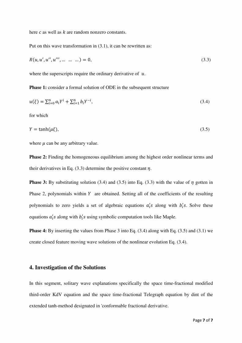
here 𝑐 as well as 𝑘 are random nonzero constants.

Put on this wave transformation in (3.1), it can be rewritten as:

𝑅(𝑢,𝑢′,𝑢′′,𝑢′′′, … … … ) = 0, (3.3)

where the superscripts require the ordinary derivative of 𝑢.

Phase 1: consider a formal solution of ODE in the subsequent structure

𝑢(𝜉) = ∑ 𝑎𝑖𝑌𝑖𝑛𝑖=0 + ∑ 𝑏𝑖𝑌−𝑖𝑛𝑖=1 , (3.4)

for which

𝑌 = tanh(𝜇𝜉), (3.5)

where 𝜇 can be any arbitrary value.

Phase 2: Finding the homogeneous equilibrium among the highest order nonlinear terms and

their derivatives in Eq. (3.3) determine the positive constant 𝜂.

Phase 3: By substituting solution (3.4) and (3.5) into Eq. (3.3) with the value of 𝜂 gotten in

Phase 2, polynomials within 𝑌 are obtained. Setting all of the coefficients of the resulting

polynomials to zero yields a set of algebraic equations 𝑎𝑖′𝑠 along with 𝑏𝑖′𝑠. Solve these

equations 𝑎𝑖′𝑠 along with 𝑏𝑖′𝑠 using symbolic computation tools like Maple.

Phase 4: By inserting the values from Phase 3 into Eq. (3.4) along with Eq. (3.5) and (3.1) we

create closed feature moving wave solutions of the nonlinear evolution Eq. (3.4).

4. Investigation of the Solutions

In this segment, solitary wave explanations specifically the space time-fractional modified

third-order KdV equation and the space time-fractional Telegraph equation by dint of the

extended tanh-method designated in 'conformable fractional derivative.

Page 8 of 8

4.1 The Space-Time Fractional Modified third order KdV Equation

The space-time fractional modified third order KdV equation is

𝐷𝑡𝛼𝑢(𝑥, 𝑡) + 𝑝𝑢2(𝑥, 𝑡)𝐷𝑥𝛽𝑢(𝑥, 𝑡) + 𝑞𝐷𝑥3𝛽𝑢(𝑥, 𝑡) = 0. 0 < 𝛼,𝛽 ≤ 1 (4.1.1)

where 𝑝, 𝑞 is a nonzero constant.

Let us consider the complex travelling waves transformation as

𝜍 = 𝜔 𝑥𝛼𝛼 − 𝜆 𝑡𝛼𝛼 , 𝑢(𝑥, 𝑡) = 𝑢(𝜍), (4.1.2)

where 𝜔, 𝜆 is the traveling wave's speed. The equation (4.1.1) is shortened to the following

integer order ordinary differential equation (ODE) through the transformation (4.1.2):

−𝜆𝑢′ + 𝜔𝑝𝑢2𝑢′ + 𝜔3𝑞𝑢′′′ = 0. (4.1.3)

Integrating equation (4.1.3) with zero constant, we achieve

3𝜔3𝑞𝑢′′ − 3𝜆𝑢 + 𝜔𝑝𝑢3 = 0. (4.1.4)

The balancing number is found 1 by balancing the highest order derivative term with the

highest power nonlinear term. The equation (3.4) is then resolved as

𝑢(𝜍) = 𝑎0 + 𝑎1𝑌 + 𝑏1𝑌−1. (4.1.5)

Take the place of (4.1.4) into (4.1.5) along with (3.5), in 𝑌, the left side converts into a

polynomial. When each of the polynomial's coefficients is set to zero, a set of algebraic

equations emerges (intended used for plainness, we try to slip over them to exposition) for 𝑎0, 𝑎1, 𝑏1,𝜔 and 𝜆 .The subsequent outcomes are attained by put on computer algebra, such as

Maple, to resolve this over determined series of equations:

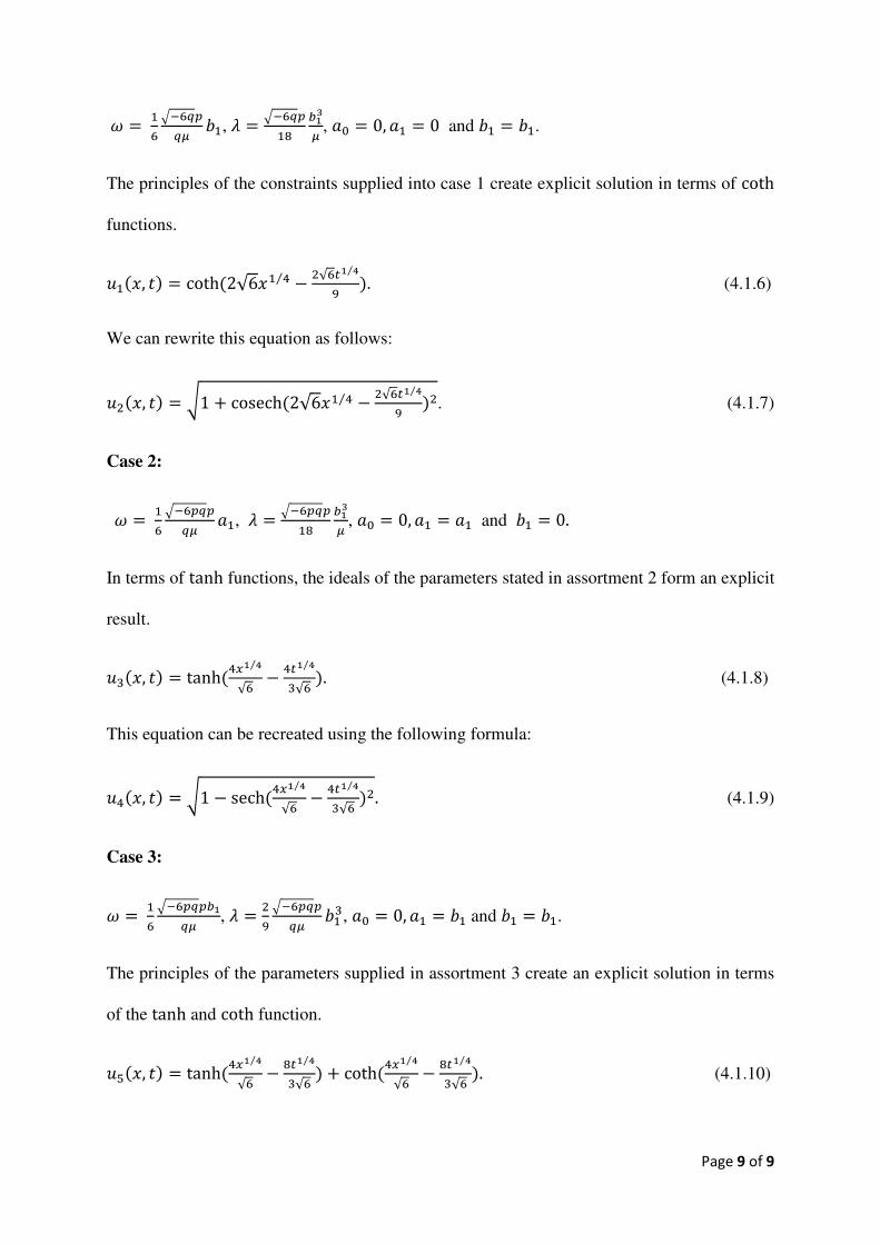
Case 1:

Page 9 of 9

𝜔 = 16 √−6𝑞𝑝𝑞𝜇 𝑏1, 𝜆 =

√−6𝑞𝑝18 𝑏13𝜇 , 𝑎0 = 0,𝑎1 = 0 and 𝑏1 = 𝑏1.

The principles of the constraints supplied into case 1 create explicit solution in terms of coth

functions.

𝑢1(𝑥, 𝑡) = coth(2√6𝑥1 4⁄ − 2√6𝑡1 4⁄9 ). (4.1.6)

We can rewrite this equation as follows:

𝑢2(𝑥, 𝑡) = √1 + cosech(2√6𝑥1 4⁄ − 2√6𝑡1 4⁄9 )2. (4.1.7)

Case 2:

𝜔 = 16 √−6𝑝𝑞𝑝𝑞𝜇 𝑎1, 𝜆 =

√−6𝑝𝑞𝑝18 𝑏13𝜇 , 𝑎0 = 0,𝑎1 = 𝑎1 and 𝑏1 = 0.

In terms of tanh functions, the ideals of the parameters stated in assortment 2 form an explicit

result.

𝑢3(𝑥, 𝑡) = tanh (4𝑥1 4⁄√6 − 4𝑡1 4⁄3√6 ). (4.1.8)

This equation can be recreated using the following formula:

𝑢4(𝑥, 𝑡) = √1 − sech(4𝑥1 4⁄√6 − 4𝑡1 4⁄3√6 )2. (4.1.9)

Case 3:

𝜔 = 16 √−6𝑝𝑞𝑝𝑏1𝑞𝜇 , 𝜆 =

29 √−6𝑝𝑞𝑝𝑞𝜇 𝑏13, 𝑎0 = 0,𝑎1 = 𝑏1 and 𝑏1 = 𝑏1.

The principles of the parameters supplied in assortment 3 create an explicit solution in terms

of the tanh and coth function.

𝑢5(𝑥, 𝑡) = tanh (4𝑥1 4⁄√6 − 8𝑡1 4⁄3√6 ) + coth (

4𝑥1 4⁄√6 − 8𝑡1 4⁄3√6 ). (4.1.10)

Page 10 of 10

The following formula can be used to reproduce this equation.

𝑢6(𝑥, 𝑡) = √1 − sech(4𝑥1 4⁄√6 − 8𝑡1 4⁄3√6 )2 + √1 + cosech(4𝑥1 4⁄√6 − 8𝑡1 4⁄3√6 )2. (4.1.11)

Case 4:

𝜔 = 16 √−6𝑝𝑞𝑏1𝑞𝜇 , 𝜆 =

19 √−6𝑝𝑞𝑝𝑞𝜇 𝑏13, 𝑎0 = 0,𝑎1= − 𝑏1 and 𝑏1 = 𝑏1.

In terms of the tanh and coth functions, the values of the parameters in assortment 4 establish

an explicit solution.

𝑢7(𝑥, 𝑡) = −tanh (4𝑥1 4⁄√6 − 4𝑡1 4⁄9 ) + coth (4𝑥1 4⁄√6 − 4𝑡1 4⁄9 ). (4.1.12)

The following formula can be used to reproduce this equation.

𝑢8(𝑥, 𝑡) = −√1 − sech (4𝑥1 4⁄√6 − 4𝑡1 4⁄9 )2 + √1 + cosech(4𝑥1 4⁄√6 − 4𝑡1 4⁄9 )2. (4.1.13)

It is striking to note that the traveling wave solutions 𝑢1 − 𝑢8 to the space-time fractional

modified third-order KdV equation are all novel also more general. These solutions recite the

circulation process of surface water waves and the electric circuit and multi constituent plasms

in fluid mechanics.

4.2 The space time fractional Telegraph equation

The suggested approach uses in this subsection to observe more universal and novel closed-

form wave solutions to the space-time fractional Telegraph equation. The space-time fractional

Telegraph equation is given by

𝐷𝑡𝑡2𝛼𝑢(𝑥, 𝑡) − 𝐷𝑥𝑥2𝛼𝑢(𝑥, 𝑡) + 𝐷𝑡𝛼𝑢(𝑥, 𝑡) + 𝛾𝑢(𝑥, 𝑡) + 𝛽𝑢3(𝑥, 𝑡) = 0. (4.2.1)

where 𝛼 is a parameter recitation the order of the fractional space and time derivative. When 𝛼 = −1 equation (4.2.1) is termed the nonlinear Telegraph equation. Exploitation the

fractional complex transform,

Page 11 of 11

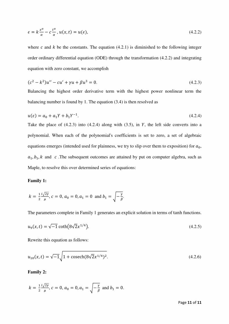
𝜖 = 𝑘 𝑥𝛼𝛼 − 𝑐 𝑡𝛼𝛼 , 𝑢(𝑥, 𝑡) = 𝑢(𝜖), (4.2.2)

where 𝑐 and 𝑘 be the constants. The equation (4.2.1) is diminished to the following integer

order ordinary differential equation (ODE) through the transformation (4.2.2) and integrating

equation with zero constant, we accomplish

(𝑐2 − 𝑘2)𝑢′′ − 𝑐𝑢′ + 𝛾𝑢 + 𝛽𝑢3 = 0. (4.2.3)

Balancing the highest order derivative term with the highest power nonlinear term the

balancing number is found by 1. The equation (3.4) is then resolved as

𝑢(𝜖) = 𝑎0 + 𝑎1𝑌 + 𝑏1𝑌−1. (4.2.4)

Take the place of (4.2.3) into (4.2.4) along with (3.5), in 𝑌, the left side converts into a

polynomial. When each of the polynomial's coefficients is set to zero, a set of algebraic

equations emerges (intended used for plainness, we try to slip over them to exposition) for 𝑎0, 𝑎1, 𝑏1,𝑘 and 𝑐 .The subsequent outcomes are attained by put on computer algebra, such as

Maple, to resolve this over determined series of equations:

Family 1:

𝑘 = 12 𝐼√2𝛾𝜇 , 𝑐 = 0, 𝑎0 = 0,𝑎1 = 0 and 𝑏1 = √− 𝛾𝛽.

The parameters complete in Family 1 generates an explicit solution in terms of tanh functions.

𝑢9(𝑥, 𝑡) = √−1 coth(8√2𝑥1 4⁄ ). (4.2.5)

Rewrite this equation as follows:

𝑢10(𝑥, 𝑡) = √−1√1 + cosech(8√2𝑥1 4⁄ )2. (4.2.6)

Family 2:

𝑘 = 12 𝐼√2𝛾𝜇 , 𝑐 = 0, 𝑎0 = 0,𝑎1 = √− 𝛾𝛽 and 𝑏1 = 0.

Page 12 of 12

In terms of tanh functions, the ideals of the parameters stated within family 2 form a plain

solution.

𝑢11(𝑥, 𝑡) = √−1 tanh(𝑥1 4⁄ √2⁄ ). (4.2.7)

This equation can be recreated using the following formula:

𝑢12(𝑥, 𝑡) = √1 − sech(𝑥1 4⁄ √2⁄ )2. (4.2.8)

Family 3:

𝑘 = 14 𝐼√2𝛾𝜇 , 𝑐 = 0, 𝑎0 = 0,𝑎1 = √− 𝛾4𝛽 and 𝑏1 =

14 𝛾√− 𝛾4𝛽.

The parameters complete in Family 3 generates an explicit solution in terms of the tanh and

coth function.

𝑢13(𝑥, 𝑡) =12 tanh (√2𝑥1 4⁄ ) +

12 coth (√2𝑥1 4⁄ ). (4.2.9)

Family 4:

𝑘 = 14 𝐼√−2𝛾+9𝛾2𝜇 , 𝑐 =

3𝛾4𝜇, 𝑎0 = √− 𝛾4𝛽 ,𝑎1 = 0 and 𝑏1 = √− 𝛾4𝛽.

In terms of tanh and coth functions, the values of the parameters in assortment 4 create an

explicit result.

𝑢14(𝑥, 𝑡) =12 +

12 coth (√7𝑥1 4⁄ − 3𝑡1 4⁄ ). (4.2.10)

The following formula can be used to reproduce this equation.

𝑢15(𝑥, 𝑡) =12 +

12√1 + cosech(√7𝑥1 4⁄ − 3𝑡1 4⁄ )2. (4.2.11)

Page 13 of 13

Family 5:

𝑘 = 14 𝐼√−2𝛾+9𝛾2𝜇 , 𝑐 = − 3𝛾4𝜇, 𝑎0 =

14 𝛾√− 𝛾4𝛽 ,𝑎1 = √− 𝛾4𝛽 and 𝑏1 = 0.

In terms of tanh and coth functions, the values of the parameters within family 4 establish an

explicit answer.

𝑢16(𝑥, 𝑡) =12 +

12 tanh (√7𝑥1 4⁄ − 3𝑡1 4⁄ ). (4.2.12)

Correspondingly

𝑢17(𝑥, 𝑡) =12 +

12√1 − sech (√7𝑥1 4⁄ − 3𝑡1 4⁄ ]2. (4.2.13)

Family 6:

𝑘 = 18 𝐼√−2𝛾+9𝛾2𝜇 , 𝑐 = − 3𝛾8𝜇, 𝑎0 =

18𝛽 𝛾√− 𝛾16𝛽 , 𝑎1 = √− 𝛾16𝛽 and 𝑏1 =116𝛽 𝛾√− 𝛾16𝛽.

The values of the parameters supplied in family 6 create an explicit solution in terms of the

tanh and coth function.

𝑢18(𝑥, 𝑡) =12 +

14 tanh(√7𝑥1 4⁄2 +

3𝑡1 4⁄2 ) +14 coth (

√7𝑥1 4⁄2 +3𝑡1 4⁄2 ). (4.2.14)

The following formula can be used to reproduce this equation.

𝑢19(𝑥, 𝑡) =12 +

14√1 − sech(√7𝑥1 4⁄2 +3𝑡1 4⁄2 )2 +

14√1 + cosech(√7𝑥1 4⁄2 +

3𝑡1 4⁄2 )2. (4.2.15)

The solutions (4.2.5)-(4.2.15) attains the mentioned equations are all new and more general

and this solutions can be explain to pulsatory blood movement among arteries also a one-

dimensional haphazard movement of bugs towards an obstacle, communication lines of all

frequencies together with direct current also high-frequency etc.

Page 14 of 14

5. Physical Description and Classification are part of the Visual

Explanation.

The physical explanation of the established traveling waves solutions to the space-time

fractional modified third-order KdV equation and the space-time fractional Telegraph

equations will be discussed in this section. The collected traveling-wave solutions of those

equations are discussed in the three-dimensional plotline, the plot of contour, and plot of vector

which are designed via Mathematica. Using those three sorts of pictorial descriptions, we may

more explicitly characterize the physical sketch.

(a) Three-dimensional

graph.

(b) Plot of contour. (c) Plot of vector.

Figure 01: Diagram of the periodic kink shape solution (4.1.6), representing (a) the three-

dimensional graph. (b) Plot of contour (c) and plot of vector of u1(x, t).

(a) Three-dimensional

graph.

(b) Plot of contour. (c) Plot of vector.

Figure 02: Diagram of the kink shape wave solution (4.1.8), representing (a) the three-dimensional

plotline (b) plot of contour (c) and plot of vector of u3(x, t).

Page 15 of 15

(a) Three-dimensional

graph.

(b) Plot of contour. (c) Plot of vector.

Figure 03: Diagram of the bell shape king wave solution (4.1.9), representing (a) the three-

dimensional plotline (b) plot of contour (c) and plot of vector of u4(x, t).

(a) Three-dimensional

graph.

(b) Plot of contour. (c) Plot of vector.

Figure 04: Diagram of the soliton king shape wave solution (4.1.12), representing (a) the

three-dimensional plotline (b) plot of contour (c) and plot of vector of u7(x, t).

(a) Three-dimensional

graph.

(b) Plot of contour. (c) Plot of vector.

Figure 05: Illustration of the anti-bell king shape wave solution (4.1.13), representing (a) the three-

dimensional plotline (b) plot of contour (c) and plot of vector of u8(𝑥, 𝑡).

Page 16 of 16

(a) Three-dimensional

graph.

(b) Plot of contour. (c) Plot of vector.

Figure 06: Illustration of the multiple soliton shape (solutions which behave at large time as

a sum of solitons) wave solution (4.2.10), representing (a) the three-dimensional plotline (b)

plot of contour (c) and plot of vector of u14(𝑥, 𝑡).

(a) Three-dimensional

graph.

(b) Plot of contour. (c) Plot of vector.

Figure 07: Illustration of the singular bell shape wave solution (4.2.11), representing (a) the

three-dimensional plotline (b) plot of contour (c) and plot of vector of u15(𝑥, 𝑡).

(a) Three-dimensional

graph.

(b) Plot of contour. (c) Plot of vector.

Figure 08: Illustration of the single soliton shape wave solution (4.2.12), representing (a) the

three-dimensional plotline (b) plot of contour (c) and plot of vector of u16(𝑥, 𝑡).

Page 17 of 17

(a) Three-dimensional

graph.

(b) Plot of contour. (c) Plot of vector.

Figure 09: Diagram of the single soliton shape wave solution (4.2.15), representing (a) the three-

dimensional plotline (b) plot of contour (c) and plot of vector of u19(𝑥, 𝑡).

sss

(a) Three-dimensional

graph.

(b) Plot of contour. (c) Plot of vector.

Figure 10: Diagram of the double solitons shape wave solution (4.2.13), representing (a) the

three-dimensional plotline (b) plot of contour (c) and plot of vector of u17(𝑥, 𝑡).

(a) Three-dimensional

graph.

(b) Plot of contour. (c) Plot of vector.

Figure 11: Diagram of the compaction wave solution (4.2.14), representing (a) the three-

dimensional plotline (b) plot of contour (c) and plot of vector of u18(𝑥, 𝑡).

Page 18 of 18

Physical clarification of the resolution

In this segment graphic delegation also physical amplification of the resolution of the derived

solutions of nonlinear fractional differential equations through the time fractional modified

third-order KdV equation and Telegraph equation are recapitulated. Solution 𝑢1(𝑥, 𝑡) in fig-1

for space-time fractional modified third-order KdV equation illustrates periodic kink shape

wave solution, within the interval −5 < 𝑥 < 10 and −5 < 𝑡 < 10 and with the values 𝜇 =

1, 𝑝 = 1, 𝑞 = −1,𝛽 =14 ,𝛼 =

14 . Periodic king wave is a recapping nonstop pattern which

regulates its wavelength and frequency. similarly, solution 𝑢2(𝑥, 𝑡) and 𝑢5(𝑥, 𝑡) delivers the

same types of solutions like periodic king wave for the values of same intervals but for the

simplicity those are omitted here. Solution u3(x, t) in fig-2 for space-time fractional modified

third-order KdV equation illustrates the kink shape wave solution with the interval 0 < 𝑥 <

100 and 0 < 𝑡 < 100 for the values 𝜇 = 1,𝑝 = 1, 𝑞 = −1,𝛽 =14 ,𝛼 =

14. Kink shape wave

solution be a wave which travels from one asymptotic spot to additional asymptotic spot wave.

Similarly, for space-time fractional Telegraph equation, solutions 𝑢6(𝑥, 𝑡), 𝑢9(𝑥, 𝑡),𝑢10(𝑥, 𝑡), 𝑢11(𝑥, 𝑡), 𝑢12(𝑥, 𝑡) for the values 𝜇 = 1,𝑝 = 1, 𝑞 = −1,𝛽 =14 ,𝛼 =

14 ,all are represent the

kink wave solution, which are hide here. In fig-3 solution u4(x, t) for space-time fractional

modified third-order KdV equation shows bell shape wave solution through the interval −10 <𝑥 < 10 and −10 < 𝑡 < 10 for the values 𝜇 = 1,𝑝 = 1, 𝑞 = −1,𝛽 =14 ,𝛼 =

14. Bell shape

wave is a continuous circulation through no breaks among principles. Fig-4 is the diagram of

the soliton king shape of u7(x, t) for the values 𝜇 = 1, 𝑝 = 1, 𝑞 = −1,𝛽 =14 ,𝛼 =

14 with the

interval 500 < 𝑥 < 100000 and 500 < 𝑡 < 100000. Soliton king shape is a confined

disorder which circulates alike a wave. Solution u8(𝑥, 𝑡) for space-time fractional modified

Page 19 of 19

third-order KdV equation shows anti-bell king wave solution for the values 𝜇 = 1,𝑝 = 1, 𝑞 =−1,𝛽 =14 ,𝛼 =

14 with the interval −1000 < 𝑥 < 10000 and −1000 < 𝑡 < 10000 in fig-5.

The solution of u14(𝑥, 𝑡) imply the type of multiple soliton shape solution, intended for the

standards 𝜇 = 1, 𝐼 = 1, 𝛾 = −1,𝛽 =14 ,𝛼 =

14 and 0 < 𝑥 < 50000, 0 < 𝑡 < 50000 is

symbolized by Fig.-6 which are represented space-time fractional Telegraph equation. The

solution of u15(𝑥, 𝑡) imply the type of singular bell shape wave solution, intended for the

standards 𝜇 = 1, 𝐼 = 1, 𝛾 = −1,𝛽 =14 ,𝛼 =

14 and 10< 𝑥 < 100, 10 < 𝑡 < 100 is

symbolized by Fig.-7. For the case of space-time fractional Telegraph equation, fig-8

demonstrates single solitons shape wave solution for the solution of u16(𝑥, 𝑡) considering the

values of 𝜇 = 1, 𝐼 = 1, 𝛾 = −1,𝛽 =14 ,𝛼 =

14 with the interval 0 < 𝑥 < 30 , 0 < 𝑡 < 30, and

also fig-9 demonstrates single solitons shape wave solution for the solution of u19(𝑥, 𝑡)considering the values of 𝜇 = 1, 𝐼 = 1, 𝛾 = −1,𝛽 =

14 ,𝛼 =14 with the interval −100 < 𝑥 <

10 , −100 < 𝑡 < 10. Singular solitons are a form of solitary wave that has a singularity, which

is typically an infinite discontinuity. When the center point of the solitary wave is imaginary,

singular solitons can be bound to it. In fig-10, the double solitons shape wave solution is

depicted, for the solution of u17(𝑥, 𝑡) (space-time fractional Telegraph equation) with the

values of 𝜇 = 1, 𝐼 = 1, 𝛾 = −1,𝛽 =14 ,𝛼 =

14 within the interval 100 < 𝑥 < −1000 and

100 < 𝑡 < −1000. Double solitons is known as a bion, or in systems where the bound state

periodically oscillates, a breather. Solution u18(𝑥, 𝑡), for space-time fractional Telegraph

equation illustrates compaction wave solution in fig-11, for the values of 𝜇 = 1, 𝐼 = 1, 𝛾 =−1,𝛽 =14 ,𝛼 =

14 with the interval −10 < 𝑥 < 0.1 and −10 < 𝑡 < 0.1. Compaction wave

solution defined as a propagating disturbance of the solid volume fraction of the granular

material.

Page 20 of 20

Conclusion

In summary, this manuscript has built scores of innovative, extra universal, and wide-ranging

solitary wave explanations employing two dependable ways relating conformable fractional

derivative, in addition, extended tanh-method to the nonlinear space time-fractional modified

third-order Kdv equation and the nonlinear space time-fractional Telegraph equation. The

obtained results illustrate that both equations accept a large number of closed-form

investigative explanations with arbitrarily conversant irreversible parameters. The recognized

outcomes reveal amusing dynamical constructions of soliton results in the categories of single

solitons, double solitons, bell types waves, kink-type waves, imaginary waves also multiple

solitons. The dynamics of solitary waves have been realistically described within relations of

space and time coordinates, revealing the reliability of the methodologies employed. The

accurateness of the data produced in these learning was confirmed by means of the

computational software Maple by re-entering them into NLFPDEs and confirming that were

correct. These soliton solutions will be beneficial in soliton theory, nonlinear wave physics,

plasma physics, optical engineering, oceanography, fluid dynamics, and engineering physics.

It is remarkable to the indication that the extended tanh-function scheme formed an extensive

assortment of computational wave solutions to the main equation. The existing technique’s

foremost benefit is that it generates more general solutions with arbitrary known-constant

constraints that also can be exerted to several categories of NLFPDEs.

Conflict of interest:

We guarantee that in this article none of the authors have any contest of interests.

Page 21 of 21

Author’s contribution

Ummay Sadia: Software, Data Curation, Writing, Formal Analysis.

Mohammad Asif Arefin: Software, Data Curation, Writing, Investigation.

Mustafa Inc: Investigation, Validation.

M. Hafiz Uddin: Conceptualization, Supervision, Writing-Reviewing Editing, Validation.

Data Availability Statements

Data sharing not applicable to this article as no datasets were generated or analyzed during

the current study.

References

[1] Du M, Wang Z, Hu H. Measuring memory with the order of fractional derivative. Sci

Rep 2013;3:1–3. https://doi.org/10.1038/srep03431.

[2] Caputo M, Fabrizio M. A new definition of fractional derivative without singular

kernel. Prog Fract Differ Appl 2015;1:73–85. https://doi.org/10.12785/pfda/010201.

[3] Zheng B. Exp-function method for solving fractional partial differential equations. Sci

World J 2013;2013. https://doi.org/10.1155/2013/465723.

[4] Čermák J, Kisela T. Stability properties of two-term fractional differential equations.

Nonlinear Dyn 2015;80:1673–84. https://doi.org/10.1007/s11071-014-1426-x.

[5] Alzai JF. The Fractional Sub-Equation Method and Exact Analytical Solutions for

Some Nonlinear Fractional PDEs. Am J Math Anal 2013;1:14–9.

https://doi.org/10.12691/ajma-1-1-3.

[6] Meng F, Feng Q. A new fractional subequation method and its applications for space-

time fractional partial differential equations. J Appl Math 2013;2013.

https://doi.org/10.1155/2013/481729.

Page 22 of 22

[7] Guo S, Mei L, Li Y, Sun Y. The improved fractional sub-equation method and its

applications to the space-time fractional differential equations in fluid mechanics. Phys

Lett Sect A Gen At Solid State Phys 2012;376:407–11.

https://doi.org/10.1016/j.physleta.2011.10.056.

[8] Feng Z. The first-integral method to study the Burgers – Korteweg – de Vries equation

n.d.;343.

[9] Younis M. The First Integral Method for Time-Space Fractional Differential

Equations. J Adv Phys 2013;2:220–3. https://doi.org/10.1166/jap.2013.1074.

[10] Meng F. A new approach for solving fractional partial differential equations. J Appl

Math 2013;2013. https://doi.org/10.1155/2013/256823.

[11] Li C, Chen A, Ye J. Numerical approaches to fractional calculus and fractional

ordinary differential equation. J Comput Phys 2011;230:3352–68.

https://doi.org/10.1016/j.jcp.2011.01.030.

[12] Varieschi GU. Applications of Fractional Calculus to Newtonian Mechanics. J Appl

Math Phys 2018;06:1247–57. https://doi.org/10.4236/jamp.2018.66105.

[13] Cui M. Compact finite difference method for the fractional diffusion equation. J

Comput Phys 2009;228:7792–804. https://doi.org/10.1016/j.jcp.2009.07.021.

[14] Huang Q, Huang G, Zhan H. A finite element solution for the fractional advection-

dispersion equation. Adv Water Resour 2008;31:1578–89.

https://doi.org/10.1016/j.advwatres.2008.07.002.

[15] El-Sayed AMA, Gaber M. The Adomian decomposition method for solving partial

differential equations of fractal order in finite domains. Phys Lett Sect A Gen At Solid

State Phys 2006;359:175–82. https://doi.org/10.1016/j.physleta.2006.06.024.

Page 23 of 23

[16] El-Sayed AMA, Behiry SH, Raslan WE. Adomian’s decomposition method for

solving an intermediate fractional advection-dispersion equation. Comput Math with

Appl 2010;59:1759–65. https://doi.org/10.1016/j.camwa.2009.08.065.

[17] Odibat Z, Momani S. A generalized differential transform method for linear partial

differential equations of fractional order. Appl Math Lett 2008;21:194–9.

https://doi.org/10.1016/j.aml.2007.02.022.

[18] He J. Variational iteration method for delay differential equations. Commun Nonlinear

Sci Numer Simul 1997;2:235–6. https://doi.org/10.1016/S1007-5704(97)90008-3.

[19] Wu G cheng, Lee EWM. Fractional variational iteration method and its application.

Phys Lett Sect A Gen At Solid State Phys 2010;374:2506–9.

https://doi.org/10.1016/j.physleta.2010.04.034.

[20] Guo S, Mei L. The fractional variational iteration method using He’s polynomials.

Phys Lett Sect A Gen At Solid State Phys 2011;375:309–13.

https://doi.org/10.1016/j.physleta.2010.11.047.

[21] Jafari H, Seifi S. Homotopy analysis method for solving linear and nonlinear fractional

diffusion-wave equation. Commun Nonlinear Sci Numer Simul 2009;14:2006–12.

https://doi.org/10.1016/j.cnsns.2008.05.008.

[22] He JH. Coupling method of a homotopy technique and a perturbation technique for

non-linear problems. Int J Non Linear Mech 2000;35:37–43.

https://doi.org/10.1016/S0020-7462(98)00085-7.

[23] Khatun MA, Arefin MA, Uddin MH. Abundant Explicit Solutions to Fractional Order

Nonlinear Evolution Equations 2021;2021.

[24] Uddin MH, Arefin MA, Akbar MA. New Explicit Solutions to the Fractional-Order

Burgers ’ Equation 2021;2021.

Page 24 of 24

[25] Uddin MH, Khatun MA, Arefin MA, Akbar MA. Abundant new exact solutions to the

fractional nonlinear evolution equation via Riemann-Liouville derivative. Alexandria

Eng J 2021;60:5183–91. https://doi.org/10.1016/j.aej.2021.04.060.

[26] Khatun MA, Asif M, Uddin MH, Baleanu D, Akbar MA. Results in Physics Explicit

wave phenomena to the couple type fractional order nonlinear evolution equations.

Results Phys 2021;28:104597. https://doi.org/10.1016/j.rinp.2021.104597.

[27] Raza N, Zubair A, Arshed S, Mahmoud EE. Optical solitons in birefringent fibers with

quadratic-cubic nonlinearity using three integration architectures 2021;025121:1–16.

https://doi.org/10.1063/5.0038038.

[28] Zhang J, Yang X. A class of efficient difference method for time fractional reaction–

diffusion equation. Comput Appl Math 2018;37:4376–96.

https://doi.org/10.1007/s40314-018-0579-5.

[29] Mophou GM. Existence and uniqueness of mild solutions to impulsive fractional

differential equations. Nonlinear Anal Theory, Methods Appl 2010;72:1604–15.

https://doi.org/10.1016/j.na.2009.08.046.

[30] Liu F, Anh V V., Turner I, Zhuang P. Time fractional advection-dispersion equation. J

Appl Math Comput 2003;13:233–45. https://doi.org/10.1007/BF02936089.

[31] Jiang W, Lin Y. Approximate solution of the fractional advection-dispersion equation.

Comput Phys Commun 2010;181:557–61. https://doi.org/10.1016/j.cpc.2009.11.004.

[32] Pandey RK, Singh OP, Baranwal VK. An analytic algorithm for the space-time

fractional advection-dispersion equation. Comput Phys Commun 2011;182:1134–44.

https://doi.org/10.1016/j.cpc.2011.01.015.

[33] Xue C, Nie J, Tan W. An exact solution of start-up flow for the fractional generalized

Burgers’ fluid in a porous half-space. Nonlinear Anal Theory, Methods Appl

Page 25 of 25

2008;69:2086–94. https://doi.org/10.1016/j.na.2007.07.047.

[34] Molliq R Y, Noorani MSM, Hashim I. Variational iteration method for fractional heat-

and wave-like equations. Nonlinear Anal Real World Appl 2009;10:1854–69.

https://doi.org/10.1016/j.nonrwa.2008.02.026.

[35] Arshed S, Biswas A, Zhou Q, Khan S, Adesanya S. Optik Optical solitons

pertutabation with Fokas-Lenells equation by exp ( − ϕ ( ξ )) -expansion method. Opt -

Int J Light Electron Opt 2019;179:341–5. https://doi.org/10.1016/j.ijleo.2018.10.136.

[36] Simulations C. The mathematics of suspensions: kac walks and asymptotic analyticity

2000:39–50.

[37] Biazar J, Ebrahimi H, Ayati Z. An Approximation to the Solution of Telegraph

Equation by Variational Iteration Method 2009. https://doi.org/10.1002/num.

[38] Yıldırım A. He ’ s homotopy perturbation method for solving the space- and time-

fractional telegraph equations 2010;7160.

https://doi.org/10.1080/00207160902874653.

[39] Avazzadeh HHZ, Machado JAT. Numerical approach for solving variable ‑ order

space – time fractional telegraph equation using transcendental Bernstein series. Eng

Comput 2019;0:0. https://doi.org/10.1007/s00366-019-00736-x.

[40] Al-shawba AA, Abdullah FA. expansion method Travelling Wave Solutions for

Fractional Boussinesq Equation Using Modified ( G ’/ G ) Expansion Method

2018;020036. https://doi.org/10.1063/1.5041567.

[41] Shah R, Farooq U, Khan H, Baleanu D, Kumam P. Fractional View Analysis of Third

Order Kortewege-De Vries Equations , Using a New Analytical Technique 2020;7:1–

11. https://doi.org/10.3389/fphy.2019.00244.

Page 26 of 26

[42] Sepehrian B, Shamohammadi Z. Arabian Journal of Mathematics A high order method

for numerical solution of time-fractional KdV equation by radial basis functions. Arab

J Math 2018;7:303–15. https://doi.org/10.1007/s40065-018-0197-5.

[43] Khalil R, Al Horani M, Yousef A, Sababheh M. A new definition of fractional

derivative. J Comput Appl Math 2014;264:65–70.

https://doi.org/10.1016/j.cam.2014.01.002.

[44] Wazwaz AM. The extended tanh method for abundant solitary wave solutions of

nonlinear wave equations. Appl Math Comput 2007;187:1131–42.

https://doi.org/10.1016/j.amc.2006.09.013.