Technical report submitted to UGC Minor Research Project Design of Optimum PID controller for Aircraft attitude control system using TAGUCHI combined Genetic Algorithm UGC Minor Research project sanction F. No. MRP-6179/15 (UGC-SERO)-dated 07-09-2016 Link NO:6179 (Technical report No. AITAM/ECE/UGC/Minor Res proj/ Venkata.L.N.Sastry.D/2017/April/1) Venkata.L.N.Sastry.D Principal Investigator Department of Electronics & Communication Engineering Aditya Institute of Technology and Management (A) Tekkali, Srikakulam-532201, A.P., India
Transcript
Technical report submitted to UGC Minor Research Project
Design of Optimum PID controller for Aircraft attitude control system
using TAGUCHI combined Genetic Algorithm
UGC Minor Research project sanction F. No. MRP-6179/15 (UGC-SERO)-dated 07-09-2016
Link NO:6179
(Technical report No. AITAM/ECE/UGC/Minor Res proj/ Venkata.L.N.Sastry.D/2017/April/1)
Venkata.L.N.Sastry.D
Principal Investigator
Department of Electronics & Communication Engineering
Aditya Institute of Technology and Management (A)
Tekkali, Srikakulam-532201, A.P., India
Contents
1.PID control theory
1.1 Role of a Proportional Controller (PC)
1.2 Role of an Integral Controller (IC)
1.3 Role of a Derivative Controller (DC)
1.4 PID controller (PID)
1.5 The transfer function of the PID controller
1.6 PID pole zero cancellation
1.7 Tuning methods
1.8 FRACTIONAL ORDER PID CONTROLLER
2. PID TUNING ALGORITHMS
2.1.Ziegler–Nichols Tuning Formula
2.2.The Wang-Juang-Chan Tuning Formula:
2.3 Optimum PID Controller design
2.4.Chien-Hrones-Reswick algorithm
2.5 Cohen-Coon algorithm
3 GENETIC ALGORITHM
3.1 Introduction
3.2 Characteristics of Genetic Algorithm
3.3 Population Size
3.4 Reproduction
3.5 Crossover
3.6 Mutation
3.7 Elitism
3.8 Objective Function Or Fitness Function
4. TAGUCHI METHOD
4.1 Introduction
4.2 Optimisation by the TAGUCHI method
5. SIMULATION & RESULTS
5.1 Optimal Design
5.2 Optimisation by the TAGUCHI method
5.3 Orthogonal array
5.4 perform the experiment
5.5 ANOM
5.6 Discussion
5.7 Optimisation by GA
5.8 Results:
5.9 Conclusion
5.10 Acknowledgement
References
List of Publications
CHAPTER-1
PID Control Theory
Introduction:
Feedback control is a control mechanism that uses information from
measurements. In a feedback control system, the output is sensed. There
are two main types of feedback control systems:
1) positive feedback
2) negative feedback.
The positive feedback is used to increase the size of the input but in a
negative feedback, the feedback is used to decrease the size of the input.
The negative systems are usually stable. A PID is widely used in feedback
control of industrial processes on the market in 1939 and has remained the
most widely used controller in process control until today. Thus, the PID
controller can be understood as a controller that takes the present, the past,
and the future of the error into consideration. After digital implementation
was introduced, a certain change of the structure of the control system was
proposed and has been adopted in many applications. But that change does
not influence the essential part of the analysis and design of PID controllers.
A proportional– integral–derivative controller (PID controller) is a method of
the control loop feedback. This method is composing of three controllers:
1. Proportional controller (PC)
2. Integral controller (IC)
3. Derivative controller (DC)
1.1 Role of a Proportional Controller (PC)
The role of a proportional depends on the present error, I on the
accumulation of past error and D on prediction of future error. The weighted
sum of these three actions is used to adjust Proportional control is a simple
and widely used method of control for many kinds of systems. In a
proportional controller, steady state error tends to depend inversely upon
the proportional gain (ie: if the gain is made larger the error goes down). The
proportional response can be adjusted by multiplying the error by a
constant Kp, called the proportional gain. The proportional term is given by:
𝑃 = 𝐾𝑃. 𝑒𝑟𝑟𝑜𝑟(𝑡) − − − (1.1)
A high proportional gain results in a large change in the output for a given
change in the error. If the proportional gain is very high, the system can
become unstable. In contrast, a small gain results in a small output
response to a large input error. If the proportional gain is very low, the
control action may be too small when responding to system disturbances.
Consequently, a proportional controller (Kp) will have the effect of reducing
the rise time and will reduce, but never eliminate, the steady-state error. In
practice the proportional band (PB) is expressed as a percentage so:
𝑃𝐵% =100
𝐾𝑃− − − − − − − (1.2)
Thus a PB of 10% ⟺ Kp=10
1.2 Role of an Integral Controller (IC)
An Integral controller (IC) is proportional to both the magnitude of the error
and the duration of the error. The integral in a PID controller is the sum of
the instantaneous error over time and gives the accumulated offset that
should have been corrected previously. Consequently, an integral control
(Ki) will have the effect of eliminating the steady-state error, but it may make
the transient response worse. The integral term is given by:
𝐼 = 𝐾𝐼 ∫ 𝑒𝑟𝑟𝑜𝑟(𝑡)𝑑𝑡 − − − − − −(1.3)𝑡
0
1.3 Role of a Derivative Controller (DC)
The derivative of the process error is calculated by determining the slope of
the error over time and multiplying this rate of change by the derivative gain
Kd. The derivative term slows the rate of change of the controller output. A
derivative control (Kd) will have the effect of increasing the stability of the
system, reducing the overshoot, and improving the transient response. The
derivative term is given by:
𝐷 = 𝐾𝐷
𝑑. 𝑒𝑟𝑟𝑜𝑟(𝑡)
𝑑𝑡− − − − − −(1.4)
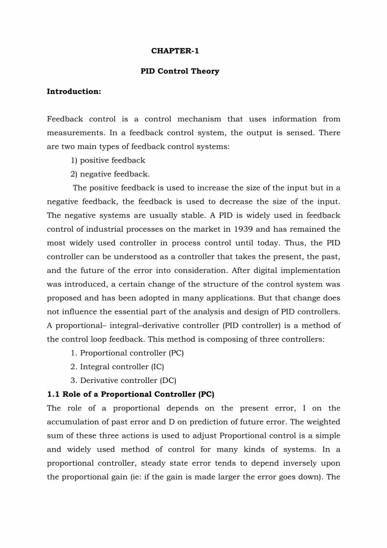
Effects of each of controllers Kp, Kd, and Ki on a closed-loop system are
summarized in the
table shown below in tableau 1.
1.4 PID controller (PID)
A typical structure of a PID control system is shown in Fig.1. Fig.2 shows a
structure of a PID control system. The error signal e(t) is used to generate
the proportional, integral, and
Table 1. A PID controller in a closed-loop system
derivative actions, with the resulting signals weighted and summed to form
the control signal u(t) applied to the plant model.
Fig.1.1: A PID control system
Fig.1.2: A structure of a PID control system
where u(t) is the input signal to the multivariable processes, the error signal
e(t) is defined as e(t) =r(t) − y(t), and r(t) is the reference input signal.
A standard PID controller structure is also known as the ‘‘three-term”
controller. This principle mode of action of the PID controller can be
explained by the parallel connection of the P, I and D elements shown in
Figure1.3.
Block diagram of the PID controller
𝐺(𝑆) = 𝐾𝑃 (1 +1 + 𝑇𝐼𝑇𝐷𝑆2
𝑇𝐼 . 𝑆) = 𝐾𝑃 (1 +
1
𝑇𝑖𝑆+ 𝑇𝐷𝑆) − − − − − −(1.5)
where KP is the proportional gain, TI is the integral time constant, TD is the
derivative time constant, KI =KP /TI is the integral gain and KD =KPTD is the
derivative gain. The ‘‘three - term” functionalities are highlighted below. The
terms KP , TI and TD definitions are:
1 The proportional term: providing an overall control action proportional to
the error signal through the all pass gain factor.
2. The integral term: reducing steady state errors through low frequency
compensation by an integrator.
3. The derivative term: improving transient response through high frequency
compensation by a differentiator.
Fig. 1.3. Parallel Form of the PID Compensator
These three variables KP , TI and TD are usually tuned within given ranges.
Therefore, they are often called the tuning parameters of the controller. By
proper choice of these tuning parameters a controller can be adapted for a
specific plant to obtain a good behaviour of the controlled system.
The time response of the controller output is
𝑢(𝑡) = 𝐾𝑃 (𝑒(𝑡) +∫ 𝑒(𝑡)𝑑𝑡
𝑡
0
𝑇𝑖+ 𝑇𝑑
𝑑𝑒(𝑡)
𝑑𝑡) − − − − − (1.6)
Using this relationship for a step input of e(t) , i.e. e(t) =δ(t) , the step
response r(t) of the PID controller can be easily determined. The result is
shown in below. One has to observe that the length of the arrow KPTD the D
action is only a measure of the weight of the δ impulse.
Fig:1. 4. a) Step response of PID ideal form b) Step response of PID real form
1.5 The transfer function of the PID controller
The transfer function of the PID controller is
𝐺(𝑆) =𝑢(𝑆)
𝐸(𝑆)− − − − − −(1.7)
𝐺(𝑆) = 𝐾𝑃 +𝐾𝐼
𝑆+ 𝐾𝐷𝑆 =
𝐾𝐷𝑆2 + 𝐾𝑃𝑆 + 𝐾𝐼
𝑆− − − − − −(1.8)
1.6 PID pole zero cancellation
The PID equation can be written in this form:
𝐺(𝑆) =𝐾𝑑 (𝑆2 +
𝐾𝑃
𝐾𝑑𝑆 +
𝐾𝑖
𝐾𝑑)
𝑆− − − − − (1.9)
When this form is used it is easy to determine the closed loop transfer
function.
𝐻(𝑆) =1
𝑆2 + 2𝜉𝜔0𝑆 + 𝜔20
− − − − − −(1.10)
If
𝐾𝑖
𝐾𝑑= 𝜔2
0 − − − − − − − − − (1.11)
𝐾𝑃
𝐾𝑑= 2𝜉𝜔0 − − − − − − − −(1.12)
Then
𝐺(𝑆)𝐻(𝑆) =𝐾𝑑
𝑆− − − − − − − −(1.13)
This can be very useful to remove unstable poles.
There are several prescriptive rules used in PID tuning. The most effective
methods generally involve the development of some form of process model,
and then choosing P, I, and D based on the dynamic model parameters.
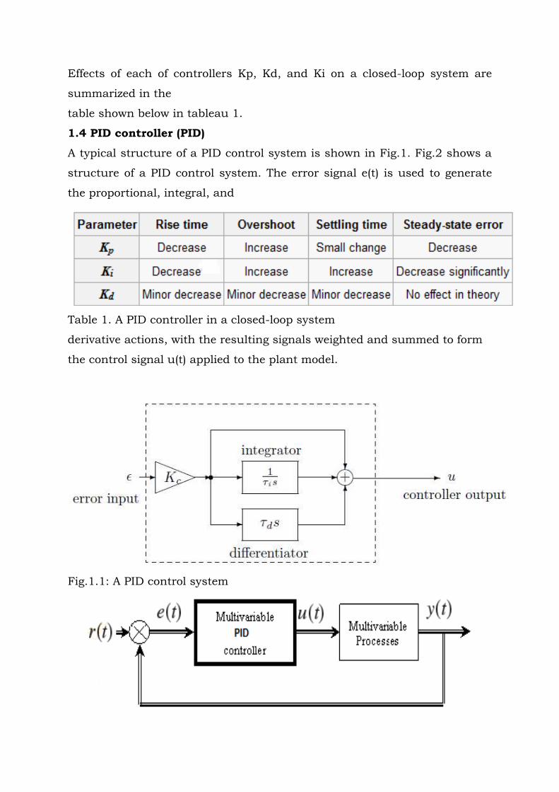
1.7 Tuning methods
We present here four tuning methods for a PID controller.
Method Advantages Disadvantages
Manuals Online method
No math expression
Requires experienced
personnel
Ziegler-Nichols Online method
Proven method
Some trial and error,
process
upset and very
aggressive
tuning
Cohen-Coon Good process models Offline method
Some math
Good only for first order
Processes
Software tools Online or offline
method,
Some cost and training
Involved
consistent tuning,
Support
Non-Steady State
tuning
Algorithmic Online or offline
method,
Consistent tuning,
Support
Non-Steady State
tuning,
Very precise
Very slow
Tuning of a PID controller refers to the tuning of its various parameters (P, I
and D) to achieve
an optimized value of the desired response. The basic requirements of the
output will be the
stability, desired rise time, peak time and overshoot. Different processes
have different
requirements of these parameters which can be achieved by meaningful
tuning of the PID
parameters. If the system can be taken offline, the tuning method involves
analysis of the step input response of the system to obtain different PID
parameters. But in most of the industrial
applications, the system must be online and tuning is achieved manually
which requires very
experienced personnel and there is always uncertainty due to human error.
Another method of
tuning can be Ziegler-Nichols method. While this method is good for online
calculations, it
involves some trial-and-error which is not very desirable.
1.8 FRACTIONAL ORDER PID CONTROLLER
1.8.1 Basic concept of Fractional order PID controller:
Consider the negative feedback control system as shown in fig
The continuous transfer function of the PI λD μ controller is obtained
through Laplace transform as
The PID controller expands the integer order PID controller from point
to plane, there by adding flexibility to controller design and allowing us to
control our real world processes more accurately but only at the cost of
increased design complexity.
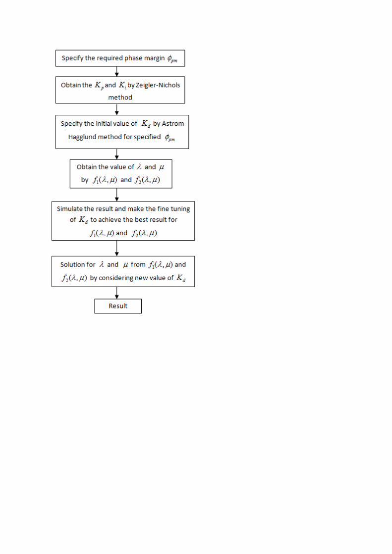
1.8.2 Tuning method for the fraction order PID controller:
To obtain the K p (proportional gain), a constant of integral term ( Ki ), the
constant of derivative term Kd, the fractional order of differentiator μ and the
fractional order of integrator λ . The method uses classical Zeigler – Nichols
tuning rule to obtain K p and Ki . To obtain initial value of Kd , then some
fine tuning has been done by using Astrom-Hagglund method described
earlier. The fractional order λ and μ are obtained to achieve specified phase
margin. Let φ pm be the required phase margin and ωcp be the frequency of
the critical point on the Nyquist curve of G(s) at which arg(G(jωcp))= -180 ,
then the gain margin defined as
In order to make the phase margin of the system equal to φ pm and |C(jωcp
)G(jωcp)=1| the following equation must be satisfied.
Then we write C (jωcp) using equation
Considering the above equations we can write
1.8.3 Algorithm for tuning of PI λ D μ controller:
CHAPTER-2
2.PID TUNING ALGORITHMS
2.1.Ziegler–Nichols Tuning Formula
A very useful empirical Tuning formula was proposed by Ziegler and
Nichols in early 1942.the tuning formula was obtained by conducting
experiment on plant or process under open loop. i.e. without connecting
controller at feed back path and step response is observed. from the step
response the parameters K,L, and T(or a where a=KL/T). with L and a the
Ziegler-Nichols formula shown in Table 2.1
Table 2.1: PID Tuning parameters by Ziegler-Nichols method
S.NO CONTROLLER
TYPE
CONTROLLER GAINS OR
VALUES
Kp Ti Td
1 P 1/a ---- ---
2 PI 0.9/a 3L ---
3 PID 1.2/a 2L L/2
2.2.The Wang-Juang-Chan Tuning Formula:
Based on the optimum ITAE criterion, the tuning algorithm proposed by
Wang, Juang, and Chan is a simple and efficient method for selecting the
PID parameters. If the k,L, T parameters of the plant model are known, the
controller parameters are given by
Kp= (𝟎.𝟕𝟑𝟎𝟑+𝟎.𝟓𝟑𝟎𝟕𝑻
𝑳⁄ )(𝑻+𝟎.𝟓𝑳)
𝑲(𝑻+𝑳)
Ti=T+0.5L Td=0.5𝐿𝑇
𝑇+0.5𝐿
2.3 Optimum PID Controller design
Optimum setting algorithms for a PID controller were proposed by Zhuang
andAtherton
for various criteria. Consider the general form of the optimum criterion
𝐽𝑛(𝜃) = ∫ [𝑡𝑛𝑒(𝜃, 𝑡)]2𝑑𝑡∞
0
where e(θ, t) is the error signal which enters the PID controller, with θ the
PID controller
parameters. For the system structure shown in Fig. 6.1, two setting
strategies are proposed:
one for the set-point input and the other for the disturbance signal d(t). In
particular, three
values of n are discussed, i.e., for n = 0, 1, 2. These three cases correspond,
respectively, to
three different optimum criteria: the integral squared error (ISE) criterion,
integral squared
time weighted error (ISTE) criterion, and the integral squared time-squared
weighted error
(ISTE) criterion. The expressions given were obtained by fitting curves to the
optimum
theoretical results.
Table 2.2: PID Tuning parameters by Optimum method
S.NO RANGE OF
L/T
0.1 – 1 1.1 - 2
CRITERION ISE ISTE IST2E ISE ISTE IST2E
1 A1 1.048 1.042 0.968 1.154 1.142 1.061
2 A2 -0.897 -0.897 -0.904 - - -0.583
0.567 0.579
3 B1 1.195 0.987 0.977 1.047 0.919 0.892
4 B2 -0.368 -0.238 -0.253 -
0.220
-
0.172
-0.165
5 A3 0.489 0.385 0.316 0.490 0.384 0.315
6 B3 0.888 0.906 0.892 0.708 0.839 0.832
For the PID controller, the gains are set as follows
𝐾𝑝 = 𝐴1
𝐾(
𝐿
𝑇)
𝐵1
𝑇𝑖 = 𝑇
𝐴2+𝐵2(𝐿𝑇⁄ )
𝑇𝑑 = 𝐴3𝑇 (𝐿
𝑇)
𝐵3
2.4.Chien-Hrones-Reswick algorithm
According to Chien-Hrones-Reswick, the tuning parameters are
𝐾𝑝 = 0.95
𝑎 ; 𝐾𝑖 =
1
2.4𝐿 ; 𝐾𝑑 = 0.42𝐿
2.5 Cohen-Coon algorithm
According to Cohen-Coon algorithm tuning parameters are
𝐾𝑝 = 1.35
𝑎(1 +
0.18µ
1 − µ)
𝐾𝑖 =1
𝑇𝑖=
2.5 − 2µ
1 − 0.39µ𝑇𝐿
𝐾𝑑 =0.37 − 0.37µ
1 − 0.81µ𝐿
CHAPTER-3
GENETIC ALGORITHM
3.1 Introduction
Genetic Algorithms (GA’ s) are a stochastic global search method that
mimics the process of natural evolution. It is one of the methods used for
optimization. John Holland formally introduced this method in the United
States in the 1970 at the University of Michigan. The continuing
performance improvements of computational systems has made them
attractive for some types of optimization. The genetic algorithm starts with
no knowledge of the correct solution and depends entirely on responses from
its environment and evolution operators such as reproduction, crossover
and mutation to arrive at the best solution. By starting at several
independent points and searching in parallel, the algorithm avoids local
minima and converging to sub optimal solutions.
3.2 Characteristics of Genetic Algorithm
Genetic Algorithms are search and optimization techniques inspired by two
biological principles namely the process of .natural selection. and the
mechanics of .natural genetics.. GAs manipulate not just one potential
solution to a problem but a collection of potential solutions. This is known
as population. The potential solution in the population is called
.chromosomes.. These chromosomes are the encoded representations of all
the parameters of the solution. Each chromosomes is compared to other
chromosomes in the population and awarded fitness rating that indicates
how successful this chromosomes to the latter. To encode better solutions,
the GA will use “genetic operators” or “evolution operators” such as
crossover and mutation for the creation of new chromosomes from the
existing ones in the population. This is achieved by either merging the
existing ones in the population or by modifying an existing chromosomes
The selection mechanism for parent chromosomes takes the fitness of the
parent into account. This will ensure that the better solution will have a
higher chance to procreate and donate their beneficial characteristic to their
offspring. genetic algorithm is typically initialized with a random population
consisting of between 20-100 individuals. This population or also known as
mating pool is usually represented by a real-valued number or a binary
string called a chromosome. For illustrative purposes, the rest of this section
represents each chromosome as a binary string. How well an individual
performs a task is measured and assessed by the objective function. The
objective function assigns
each individual a corresponding number called its fitness. The fitness of
each chromosome is assessed and a survival of the fittest strategy is
applied. In this project, the magnitude of the error will be used to assess the
fitness of each chromosome. There are three main stages of a genetic
algorithm, these are known as reproduction, crossover and mutation. This
will be explained in details in the following section
3.3 Population Size
Determining the number of population is the one of the important step in
GA.There are many research papers that dwell in the subject. Many theories
have been documented and experiments recorded However the matter of the
fact is that more and more theories and experiments are conducted and
tested and there is no fast and thumb rule with regards to which is the best
method to adopt. For a long time the decision on the population size is
based on trial and error. In this project the approach in determining the
population is rather unsciencetific. From my reading of various papers, it
suggested that the safe population size is from 30 to 100. In this project an
initial population of 20 were used and the result observed. The result was
not promising. Hence an initiative of 40, 60, 80 and 90 size of population
were experimented. It was observed that the population of 80 seems to be a
good guess. Population of 90 and above does not results in any further
optimization.
3.4 Reproduction
During the reproduction phase the fitness value of each chromosome is
assessed. This value is used in the selection process to provide bias towards
fitter individuals. Just like in natural evolution, a fit chromosome has a
higher probability of being selected for reproduction. An example of a
common selection technique is the .Roulette Wheel selection method . Each
individual in the population is allocated a section of a roulette wheel. The
size of the section is proportional to the fitness of the individual. A pointer is
spun and the individual to whom it points is selected. This continues until
the selection criterion has been met. The probability of an individual being
selected is thus related to its fitness, ensuring that fitter individuals are
more likely to leave offspring. Multiple copies of the same string may be
selected for reproduction and the fitter strings should begin to dominate.
However, for the situation illustrated in Figure 8, it is not implausible for the
weakest string (01001) to dominate the selection process. There are a
number of other selection methods available and it is up to the user to select
the appropriate one for each process. All selection methods are based on the
same principal that is giving fitter chromosomes a larger probability of
selection.
Four common methods for selection are:
1. Roulette Wheel selection
2. Stochastic Universal sampling
3. Normalized geometric selection
4. Tournament selection
Due to the complexities of the other methods, the Roulette Wheel methods is
preferred in this project.
3.5 Crossover
Once the selection process is completed, the crossover algorithm is initiated.
The crossover operations swaps certain parts of the two selected strings in a
bid to capture the good parts of old chromosomes and create better new
ones. Genetic operators manipulate the characters of a chromosome
directly, using the assumption that certain individual.s gene codes, on
average, produce fitter individuals. The crossover probability indicates how
often crossover is performed. A probability of 0% means that the .offspring.
will be exact replicas of their
.parents. and a probability of 100% means that each generation will be
composed of entirely new offspring. The simplest crossover technique is the
Single Point Crossover.
There are two stages involved in single point crossover:
1. Members of the newly reproduced strings in the mating pool are .mated.
(paired) at random.
2. Each pair of strings undergoes a crossover as follows: An integer k is
randomly selected between one and the length of the string less one, [1,L-1].
Swapping all the characters between positions k+1 and L inclusively creates
two new strings.
Example: If the strings 10000 and 01110 are selected for crossover and the
value
of k is randomly set to 3 then the newly created strings will be 10010 and
01100
More complex crossover techniques exist in the form of Multi-point and
Uniform Crossover Algorithms. In Multi-point crossover, it is an extension of
the single point crossover algorithm and operates on the principle that the
parts of a chromosome that contribute most to its fitness might not be
adjacent. There are three main stages involved in a Multi-point crossover.
1. Members of the newly reproduced strings in the mating pool are .mated.
(paired) at random.
2. Multiple positions are selected randomly with no duplicates and sorted
into ascending order.
3. The bits between successive crossover points are exchanged to produce
new offspring.
3.6 Mutation
Using selection and crossover on their own will generate a large amount of
different strings. However there are two main problems with this:
1. Depending on the initial population chosen, there may not be enough
diversity in the initial strings to ensure the Genetic Algorithm searches the
entire problem space.
2. The Genetic Algorithm may converge on sub-optimum strings due to a
bad choice of initial population.
3.7 Elitism
In the process of the crossover and mutation-taking place, there is high
chance that the optimum solution could be lost. There is no guarantee that
these operators will preserve the fittest string. To avoid this, the elitist
models are often used. In this model, the best individual from a population
is saved before any of these operations take place. When a new population is
formed and evaluated, this model will examine to see if this best structure
has been preserved. If not the saved copy is reinserted into the population.
The GA will then continues on as normal.
3.8 Objective Function Or Fitness Function
The objective function is used to provide a measure of how individuals have
performed in the problem domain. In the case of a minimization problem,
the most fit individuals will have the lowest numerical value of the
associated objective function. This raw measure of fitness is usually only
used as an intermediate stage in determining the relative performance of
individuals in a GA.
Another function that is the fitness function, is normally used to transform
the objective function value into a measure of relative fitness, thus where f is
the objective function, g transforms the value of the objective function to a
nonnegative number and F is the resulting relative fitness. This mapping is
always necessary when the objective function is to be minimized as the
lower objective function values correspond to fitter individuals. In many
cases, the fitness function value corresponds to the number of offspring that
an individual can
expect to produce in the next generation. A commonly used transformation
is that of proportional fitness assignment.
CHAPTER-4
TAGUCHI METHOD
4.1 Introduction
The Taguchi method is an optimization method. This method has been
applied to solve many optimization problems in electrical machines design
and electric power systems . It does not need to use sophisticated algorithms
and extra programming besides the software tool used for system modeling .
For the same number of design variables and levels, the Taguchi method
gives a lower number of design experiments than that of the response
surface methodology. Therefore, time saving and lower cost can be achieved
by using this method. However, the Taguchi method is sufficient to deal with
multiobjective optimization problems requiring more than two factors, but
the Taguchi method can be combined with another technique to obtain
accurate results.
`
4.2 Optimisation by the TAGUCHI method
The Taguchi method was constructed based on the principle of an
orthogonal array that can effectively minimize the number of design
experiments required in any design process. The Taguchi method can
provide an efficient way to obtain the optimal parameters in an optimization
problem. In the Taguchi method, an orthogonal array that depends on the
number of factors and their levels is used to study the parameters’ variation
effect. This method has a low number of experiments. For example, if there
are four factors each at three levels, the full factorial design method requires
34 = 81 experiments while the Taguchi method needs only nine experiments
to obtain the approximate optimal values.
4.2.1 Orthogonal Array
In establishing an orthogonal array, four factors A, B, C, and D are
considered. A is the proportional gain, B is the integral gain, C is the
derivative gain, and D is the saturation limit of an integral action. The
saturation limit fixes 100 for the AVR system stability. Table II illustrates
the design variables
or factors and their levels. The standard Taguchi’s orthogonal array L-9 is
used for this numerical experiments study.
4.2.2 perform the experiment
Nine experiments should be carried out in order to know the dynamic
response of the AVR system with the PID controller at combination levels of
these factors. The maximum percentage overshoot (MPOS), the rise time (T
r), the settling time (T s), and the steady-state error (Ess) of the terminal
voltage of a synchronous generator are the most important variables. To
obtain the values of MPOS, T r , T s, and Ess for each experiment, the
MATLAB-Simulink model of the AVR system with the PID controller is used.
After performing the nine experiments and obtaining all experimental data,
ANOM and ANOVA are carried out to estimate the effects of the three design
parameters and to determine the relative importance of each design
parameter, respectively.
4.2.3 ANOM
1) Overall Mean: The mean or average value of all results can be
calculated as follows:
𝑚 = 1
9∑ 𝑀𝑃𝑂𝑆𝑖
9
𝑖=1
2) Average Effect of a Design Variable at One Setting: The MPOS of factor
A at level three is calculated by
𝑚𝐴3(𝑀𝑃𝑂𝑆) = 1
3(𝑀𝑃𝑂𝑆(7) + 𝑀𝑃𝑂𝑆(8) + 𝑀𝑃𝑂𝑆(9))
where the factor A is set to level three only in experiments . The MPOS for all
levels for all factors can be determined by a similar way In a similar way, T r
, T s, and Ess can be obtained for all levels of all factorsIt can be realized
that the factor-level combination (A3, B1, C1) contributes to minimization of
T r , T s, and Ess.
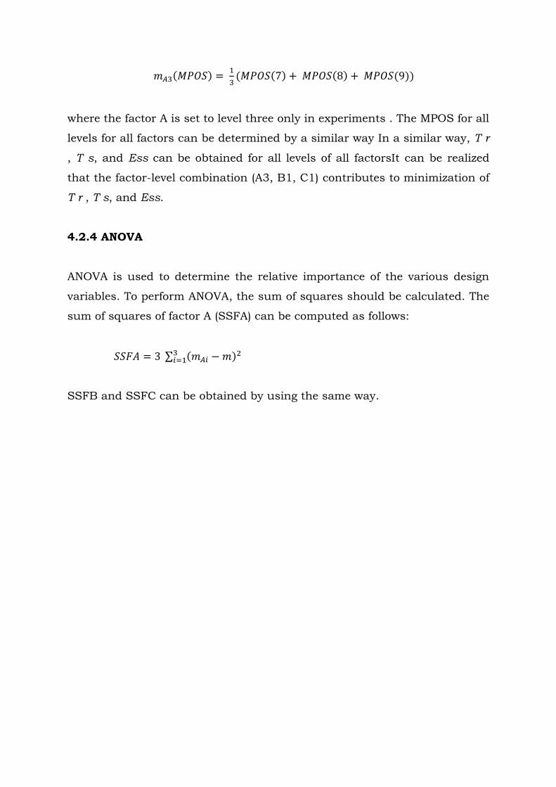
4.2.4 ANOVA
ANOVA is used to determine the relative importance of the various design
variables. To perform ANOVA, the sum of squares should be calculated. The
sum of squares of factor A (SSFA) can be computed as follows:
𝑆𝑆𝐹𝐴 = 3 ∑ (𝑚𝐴𝑖 − 𝑚)23𝑖=1
SSFB and SSFC can be obtained by using the same way.
CHAPTER-5
SIMULATION & RESULTS
5.1 Optimal Design
The design optimization process is presented in this paper for optimizing the
PID controller parameters using the TCGA method. This method refers to
the accurate optimum design
that improves the dynamic response of the Aircraft attitude system.
However, the procedure for the optimal design consists of two main steps. In
the first step, the optimization is carried out by the Taguchi method in order
to obtain the approximate optimal values of the PID controller parameters
using ANOM. Then, ANOVA is used to choose the design variables
influencing the objective function. In the second step, a multiobjective GA is
carried out to find the accurate optimum values of these influential design
variables. The proposed optimization method has many merits. In the
Taguchi method, the number of design experiments is reduced in
comparison with the full factorial design. Moreover, by using ANOVA to
select the influential design variables, the design area for optimization using
GA is greatly reduced
5.2 Optimisation by the TAGUCHI method
The Taguchi method was constructed based on the principle of an
orthogonal array that can effectively minimize the number of design
experiments required in any design process. The Taguchi method can
provide an efficient way to obtain the optimal parameters in an optimization
problem. In the Taguchi method, an orthogonal array that depends on the
number of factors and their levels is used to study the parameters’ variation
effect This method has a low number of experiments. For example, if there
are four factors each at three levels, the full factorial design method requires
34 = 81 experiments while the Taguchi method needs only nine experiments
to obtain the approximate optimal values.
5.3 Orthogonal array
In establishing an orthogonal array, four factors X, Y, Z are considered. X is
the proportional gain, Y is the integral gain, and Z is the derivative gain.
Table 5.1 illustrates the design variables or factors and their levels. The
standard Taguchi’s orthogonal array L-9 is used for this numerical
experiments study, as shown in Table 5.2
Table 5.1: Design Variables and Levels
Design
variable Level 1 Level 2 Level 3
X 6 7 8
Y 0.5 0.6 0.7
Z 0.2 0.25 0.3
Table 5.2: Actual Values of Three Settings of Three Design Variables
EXP.NO X Y Z
1 6 0.5 0.2
2 6 0.6 0.25
3 6 0.7 0.3
4 7 0.5 0.25
5 7 0.6 0.3
6 7 0.7 0.2
7 8 0.5 0.3
8 8 0.6 0.2
9 8 0.7 0.25
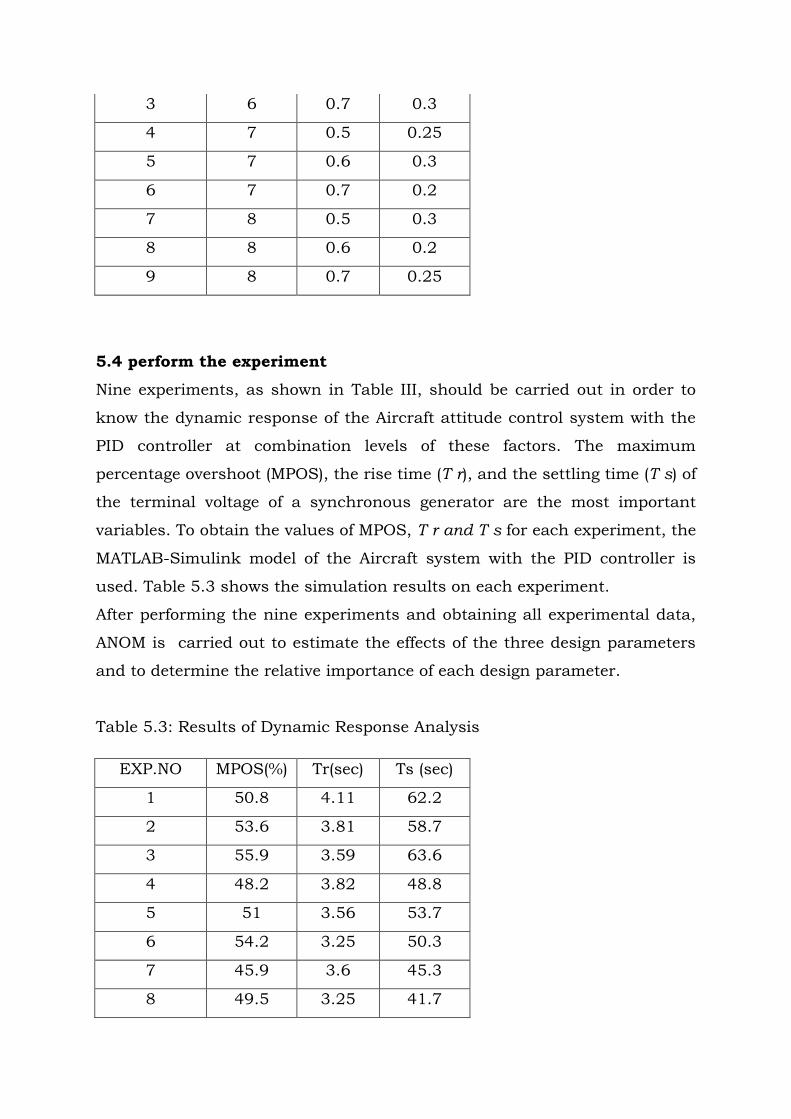
5.4 perform the experiment
Nine experiments, as shown in Table III, should be carried out in order to
know the dynamic response of the Aircraft attitude control system with the
PID controller at combination levels of these factors. The maximum
percentage overshoot (MPOS), the rise time (T r), and the settling time (T s) of
the terminal voltage of a synchronous generator are the most important
variables. To obtain the values of MPOS, T r and T s for each experiment, the
MATLAB-Simulink model of the Aircraft system with the PID controller is
used. Table 5.3 shows the simulation results on each experiment.
After performing the nine experiments and obtaining all experimental data,
ANOM is carried out to estimate the effects of the three design parameters
and to determine the relative importance of each design parameter.
Table 5.3: Results of Dynamic Response Analysis
EXP.NO MPOS(%) Tr(sec) Ts (sec)
1 50.8 4.11 62.2
2 53.6 3.81 58.7
3 55.9 3.59 63.6
4 48.2 3.82 48.8
5 51 3.56 53.7
6 54.2 3.25 50.3
7 45.9 3.6 45.3
8 49.5 3.25 41.7
9 51.7 3.07 46.7
5.5 ANOM
i) Overall Mean: The mean or average value of all results can be
calculated as follows:
𝑚 = 1
9 ∑ 𝑀𝑃𝑂𝑆𝑖
𝑝𝑖=1
Table 5.4 shows the mean of MPOS, T r , and T s.
Table 5.4: Mean of Results
MPOS(%) Tr(sec) Tssec)
m (overall
mean) 51.2 3.56 52.33
ii) Average Effect of a Design Variable at One Setting:
The MPOS of factor A at level three is calculated by
mx3 (MPOS) =1/3 (MPOS(7)+MPOS(8)+MPOS(9))
where the factor X is set to level three only in experiments 7–9. The MPOS
for all levels for all factors can be determined by a similar way. The results
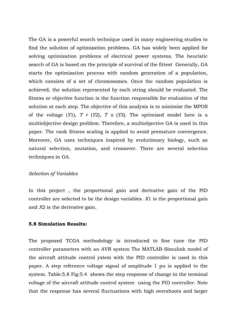
are given in Table:5.5. Fig.5.1 shows main factor effects on the MPOS. It
can be noticed that the factor-level combination (X1, Y1,Z3) contributes to
minimization of the MPOS.
Table 5.5: MPOS for All Levels of All Factors
settings of
factor
MPOS of
X
MPOS of
Y
MPOS of
Z
1 53.33 48.3 51.5
2 51.13 51.36 51.16
3 49.03 53.93 50.93
Fig 5.1: Main factors effects on the MPOS
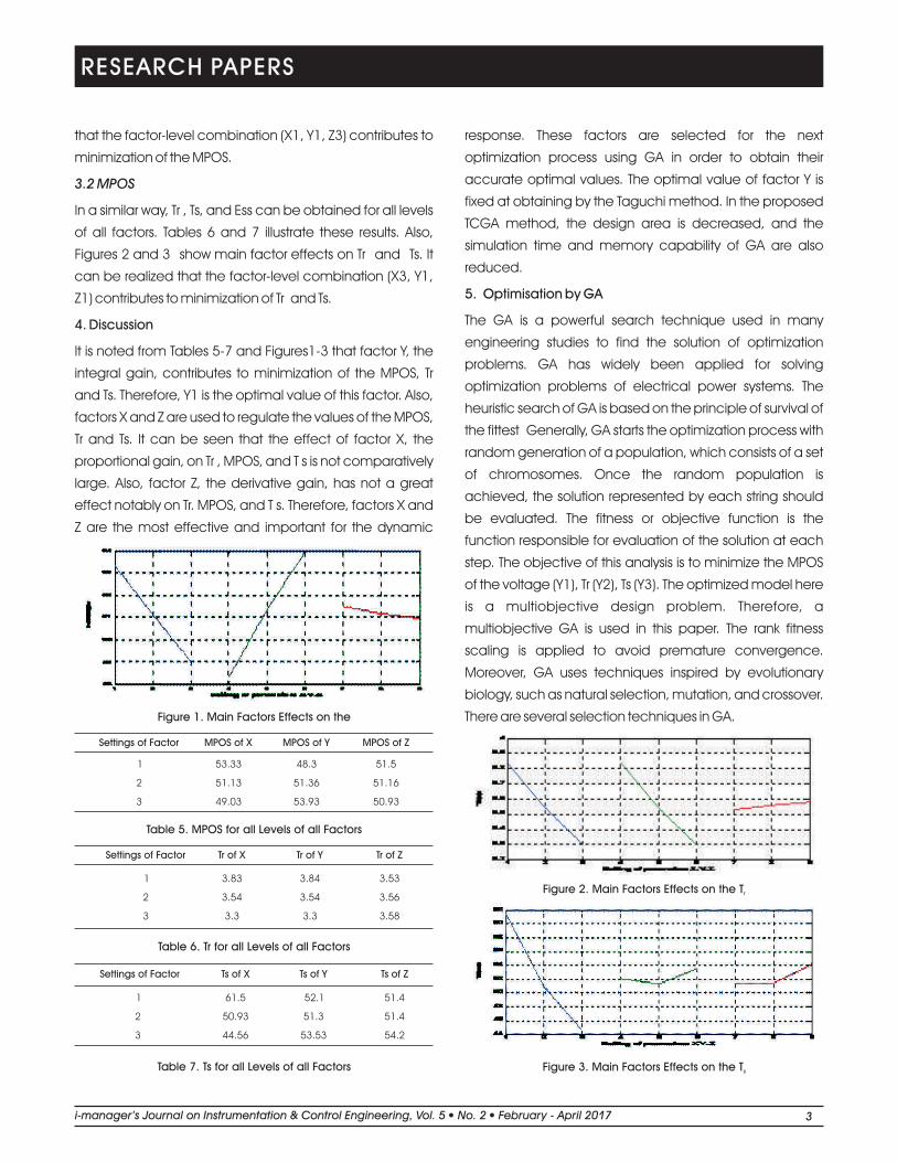
In a similar way, T r , T s, and Ess can be obtained for all levels of all factors.
Tables 5.6&5.7 illustrate these results. Also, Figs.5.2 &5.3 show main
factor effects on T r and T s. It can be realized that the factor-level
combination (X3, Y1, Z1) contributes to minimization of T r and T s,
Table:5.6 Tr for All Levels of All Factors
settings of
factor Tr of X Tr of Y Tr of Z
1 3.83 3.84 3.53
2 3.54 3.54 3.56
3 3.3 3.3 3.58
Table:5.7 Ts for All Levels of All Factors
settings of
factor Ts of X Ts of Y Ts of Z
1 61.5 52.1 51.4
2 50.93 51.3 51.4
3 44.56 53.53 54.2
1 2 3 4 5 6 7 8 948
49
50
51
52
53
54
Setting of parameters X,Y,Z
MPOS
(%)
Fig:5.2 Main factors effects on the Tr
Fig:5.3 Main factors effects on the Ts
5.6 Discussion
It is noted from Tables VI–IX and Figs. 2–5 that factor Y, the integral gain,
contributes to minimization of the MPOS, T r and T s. Therefore, Y1 is the
optimal value of this factor. Also, factors X and Z are used to regulate the
values of the MPOS, T r and T s. It can be seen that the effect of factor X,
the proportional gain, on T r , MPOS, and T s is not comparatively large.
Also, factor Z, the derivative gain, has not a great effect notably on T r .
MPOS, and T s. Therefore, factors X and Z are the most effective and
important for the dynamic response. These factors are selected for the next
optimization process using GA in order to obtain their accurate optimal
values. The optimal value of factor Y is fixed at obtaining by the Taguchi
method. In the proposed TCGA method, the design area is decreased, and
the simulation time and memory capability of GA are also reduced.
5.7 Optimisation by GA
1 2 3 4 5 6 7 8 93.2
3.3
3.4
3.5
3.6
3.7
3.8
3.9
4
Setting of parameters X,Y,Z
Tr(sec
)
1 2 3 4 5 6 7 8 944
46
48
50
52
54
56
58
60
62
Setting of parameters X,Y,Z
Ts(sec
)
The GA is a powerful search technique used in many engineering studies to
find the solution of optimization problems. GA has widely been applied for
solving optimization problems of electrical power systems. The heuristic
search of GA is based on the principle of survival of the fittest Generally, GA
starts the optimization process with random generation of a population,
which consists of a set of chromosomes. Once the random population is
achieved, the solution represented by each string should be evaluated. The
fitness or objective function is the function responsible for evaluation of the
solution at each step. The objective of this analysis is to minimize the MPOS
of the voltage (Y1), T r (Y2), T s (Y3). The optimized model here is a
multiobjective design problem. Therefore, a multiobjective GA is used in this
paper. The rank fitness scaling is applied to avoid premature convergence.
Moreover, GA uses techniques inspired by evolutionary biology, such as
natural selection, mutation, and crossover. There are several selection
techniques in GA.
Selection of Variables
In this project , the proportional gain and derivative gain of the PID
controller are selected to be the design variables. X1 is the proportional gain
and X2 is the derivative gain.
5.8 Simulation Results:
The proposed TCGA methodology is introduced to fine tune the PID
controller parameters with an AVR system The MATLAB-Simulink model of
the aircraft attitude control ystem with the PID controller is used in this
paper. A step reference voltage signal of amplitude 1 pu is applied to the
system. Table:5.8 Fig:5.4 shows the step response of change in the terminal
voltage of the aircraft attitude control system using the PID controller. Note
that the response has several fluctuations with high overshoots and larger
settling time. The MPOS reduced by12.3%, the T r reduces by 0.6 s, the T s
reduces by 17.3 s.
Table:5.8 Comparision between PID and GA-PID
parameters PID GA-PID
MPOS(%) 54 41.7
Tr (sec) 2.89 2.29
Ts (sec) 44.4 27.1
Fig:5.4 Comparison of step responses of PID with proposed method.
5.9 Conclusion
In this project, a novel Taguchi combined genetic algorithm method was
presented to optimally design a PID controller in the aircraft attitude control
system for improving the step response of attitude voltage. The proportional
gain, the integral gain and the derivative gain were chosen to define the
search space for the optimization problem. The near optimum values of the
design variables were determined by the Taguchi method using analysis of
means. Analysis of variance was used to select the two most influential
design variables. As a result of the proposed approach, fast design and an
accurate performance prediction was achieved. Therefore, when this
0 10 20 30 40 50 60 700
0.5
1
1.5
2
Step Response
Time (seconds)
aircr
aft a
ttitu
de p
ositio
n
PID
0 5 10 15 20 25 30 35 40 450
0.5
1
1.5
Step Response
Time (seconds)
aircr
aft a
ttitu
de p
ositio
n
GA-PID
proposed approach is applied, it is more efficient in raising the precision of
optimization.
5.10 Acknowledgement
The author would like to thank the UGC Delhi for granting funding for
minor research project.
References
[1] A. H. M. S. Ula and A. R. Hasan, “Design and implementation of a
personal computer based automatic voltage regulator for a synchronous
generator,” IEEE Trans. Energy Convers., vol. 7, no. 1, pp. 125–131, Mar.
1992.
[2] K. J. Astrom and T. Hagglund, “The future of PID control,” Control Eng.
Practice, vol. 9, no. 11, pp. 1163–1175, 2001.
[3] A. Visioli, “Tuning of PID controllers with fuzzy logic,” IEE Proc. Control
Theory Appl., vol. 148, no. 1, pp. 1–8, Jan. 2001.
[4] Y. Li, K. H. Ang, and G. C. Y. Chong, “PID control system analysis and
design, problems, remedies, and future directions,” IEEE Control Syst. Mag.,
vol. 26, no. 1, pp. 32–41, 2006.
[5] S.-R. Qi, D.-F. Wang, P. Han, and Y.-H. Li, “Grey prediction based RBF
neural network self-tuning PID control for turning process,” in Proc. Int.
Conf. Mach. Learning Cybern., 2004, pp. 802–805.
[6] A. Rubaai, M. J. Castro-Sitiriche, and A. R. Ofoli, “Design and
implementation of parallel fuzzy PID controller for high-performance
brushless motor drives: An integrated environment for rapid control