1 N. Gauger et al. Intro to Optimization and MDO, VKI, March 6-10,2006 Adjoint Approaches in Aerodynamic Shape Optimization and MDO Context I/II Nicolas Gauger 1), 2) 1) DLR Braunschweig Institute of Aerodynamics and Flow Technology Numerical Methods Branch 2) Humboldt University Berlin Department of Mathematics Introduction to Optimization and Multidisciplinary Design VKI, March 6-10, 2006 http://www.mathematik.hu-berlin.de/~gauger
Transcript
1N. Gauger et al.Intro to Optimization and MDO, VKI, March 6-10,2006
Adjoint Approaches in Aerodynamic Shape Optimization and MDO Context I/II
Nicolas Gauger 1), 2)
1) DLR BraunschweigInstitute of Aerodynamics and Flow Technology
Numerical Methods Branch2) Humboldt University Berlin
Department of Mathematics
Introduction to Optimization and Multidisciplinary DesignVKI, March 6-10, 2006
http://www.mathematik.hu-berlin.de/~gauger
2N. Gauger et al.Intro to Optimization and MDO, VKI, March 6-10,2006
CollaboratorsWith contributions to this lecture:
• DLR: N. Kroll, J. Brezillon, A. Fazzolari,
R. Dwight, M. Widhalm
• HU Berlin: A. Griewank, J. Riehme
• Fastopt: R. Giering, Th. Kaminski
• TU Dresden: A. Walther, C. Moldenhauer
• Uni Trier: V. Schulz, S. HazraUniversity of Trier
FastOpt
3N. Gauger et al.Intro to Optimization and MDO, VKI, March 6-10,2006
Content of lecture
Why adjoint approaches?
What is an adjoint approach?
Continuous and discrete adjoint approaches / solvers
Validation and Application in 2D and 3D, Euler and Navier-Stokes
Algorithmic / Automated Differentiation (AD)
Coupled aero-structure adjoint approach
Validation and application in MDO context
One shot approaches
4N. Gauger et al.Intro to Optimization and MDO, VKI, March 6-10,2006
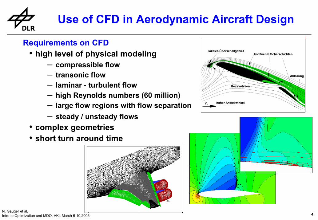
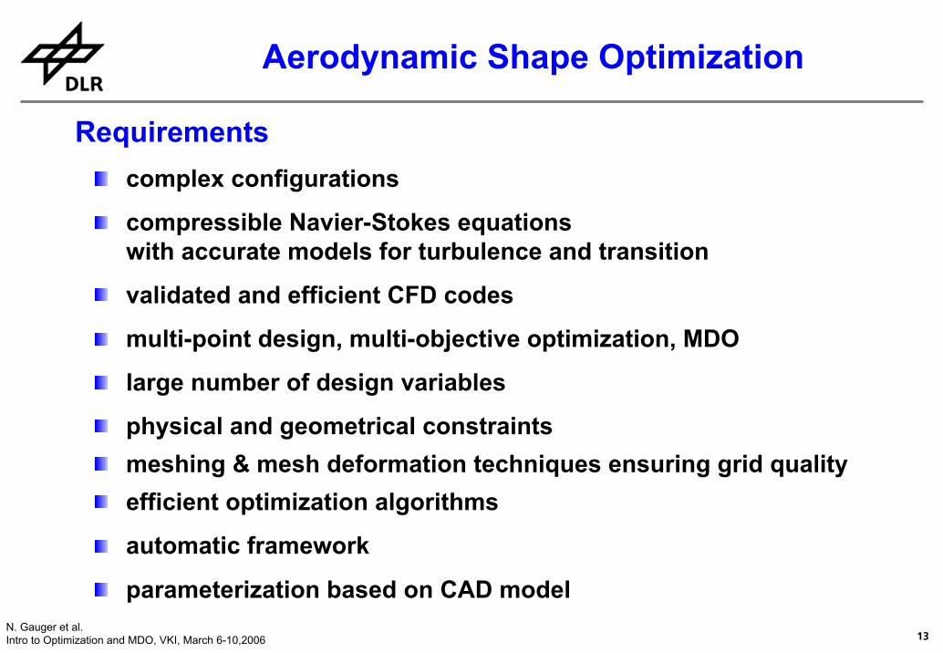
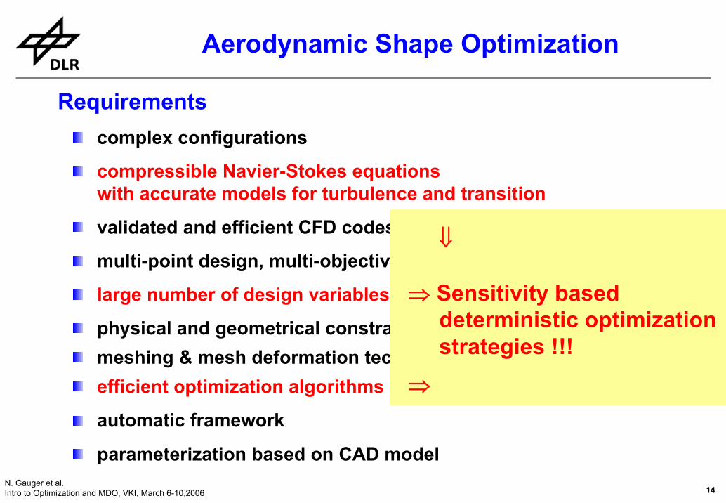
Requirements on CFD• high level of physical modeling
– compressible flow– transonic flow– laminar - turbulent flow – high Reynolds numbers (60 million)– large flow regions with flow separation – steady / unsteady flows
• complex geometries• short turn around time
Use of CFD in Aerodynamic Aircraft Design
5N. Gauger et al.Intro to Optimization and MDO, VKI, March 6-10,2006
Consequencessolution of 3D compressible Reynolds averaged Navier-Stokes equations turbulence models based on transport equations (2 – 6 eqn)models for predicting laminar-turbulent transition flexible grid generation techniques with high level of automation(block structured grids, overset grids, unstructured/hybrid grids)link to CAD-systemsefficient algorithms (multigrid, grid adaptation, parallel algorithms...)large scale computations ( ~ 10 - 25 million grid points)…
Use of CFD in Aerodynamic Aircraft Design
6N. Gauger et al.Intro to Optimization and MDO, VKI, March 6-10,2006
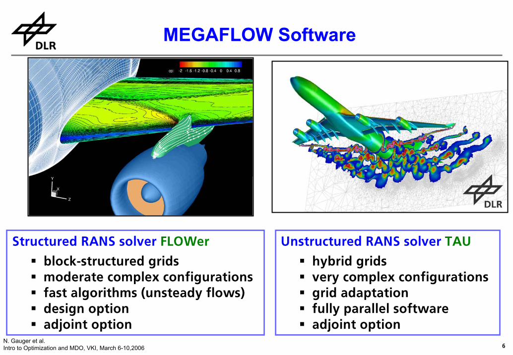
hybrid grids very complex configurationsgrid adaptation fully parallel softwareadjoint option
7N. Gauger et al.Intro to Optimization and MDO, VKI, March 6-10,2006
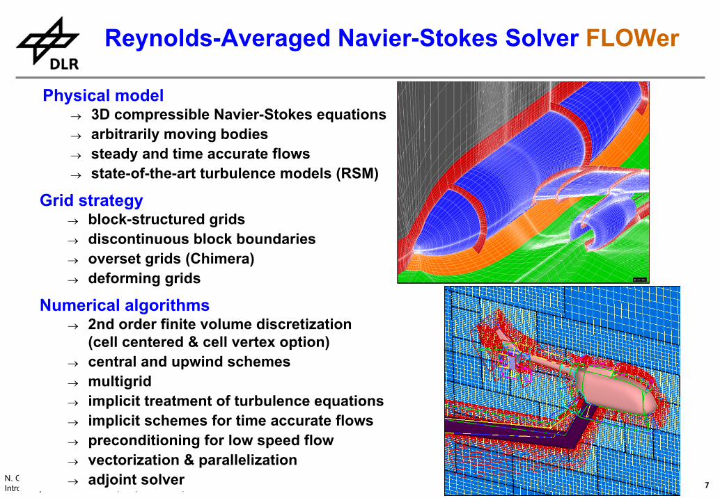
Physical model→ 3D compressible Navier-Stokes equations→ arbitrarily moving bodies→ steady and time accurate flows→ state-of-the-art turbulence models (RSM)
Reynolds-Averaged Navier-Stokes Solver FLOWer
Numerical algorithms→ 2nd order finite volume discretization
(cell centered & cell vertex option)→ central and upwind schemes→ multigrid→ implicit treatment of turbulence equations→ implicit schemes for time accurate flows→ preconditioning for low speed flow→ vectorization & parallelization→ adjoint solver
8N. Gauger et al.Intro to Optimization and MDO, VKI, March 6-10,2006
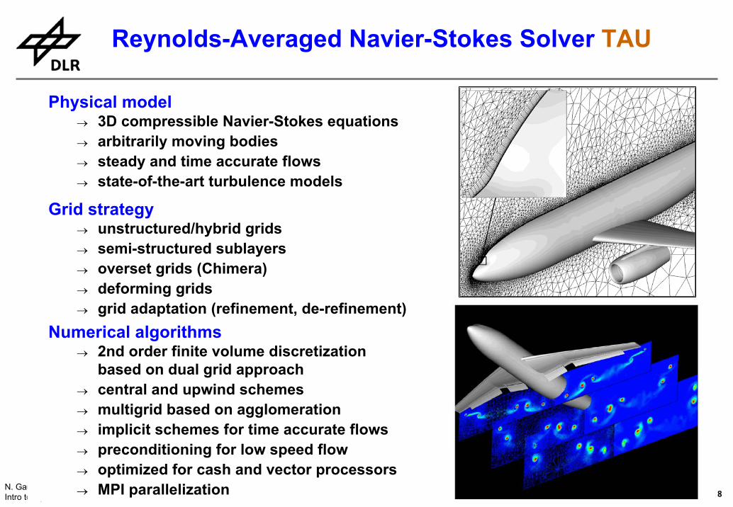
Physical model→ 3D compressible Navier-Stokes equations→ arbitrarily moving bodies→ steady and time accurate flows→ state-of-the-art turbulence models
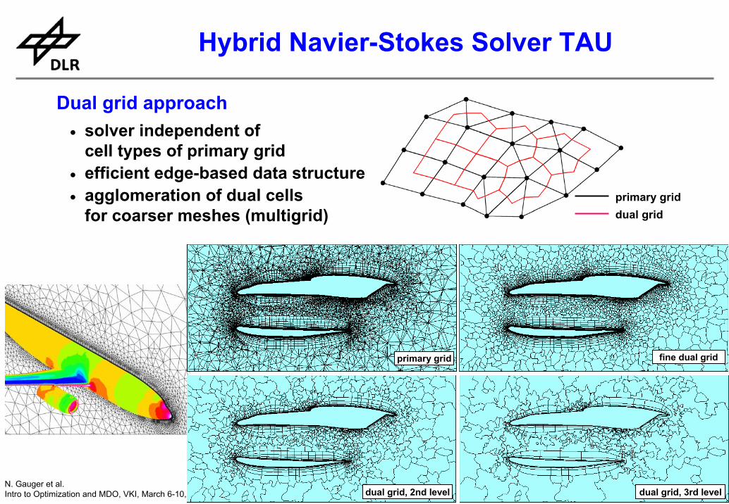
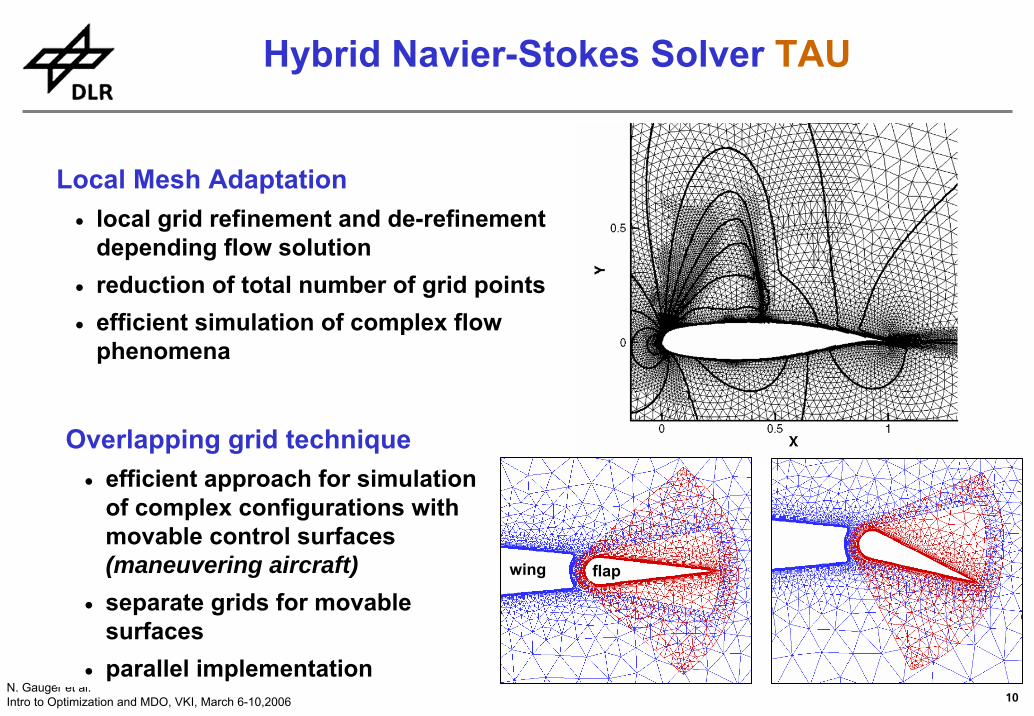
Reynolds-Averaged Navier-Stokes Solver TAU
Numerical algorithms→ 2nd order finite volume discretization
based on dual grid approach→ central and upwind schemes→ multigrid based on agglomeration → implicit schemes for time accurate flows→ preconditioning for low speed flow→ optimized for cash and vector processors→ MPI parallelization
19N. Gauger et al.Intro to Optimization and MDO, VKI, March 6-10,2006
20N. Gauger et al.Intro to Optimization and MDO, VKI, March 6-10,2006
21N. Gauger et al.Intro to Optimization and MDO, VKI, March 6-10,2006
22N. Gauger et al.Intro to Optimization and MDO, VKI, March 6-10,2006
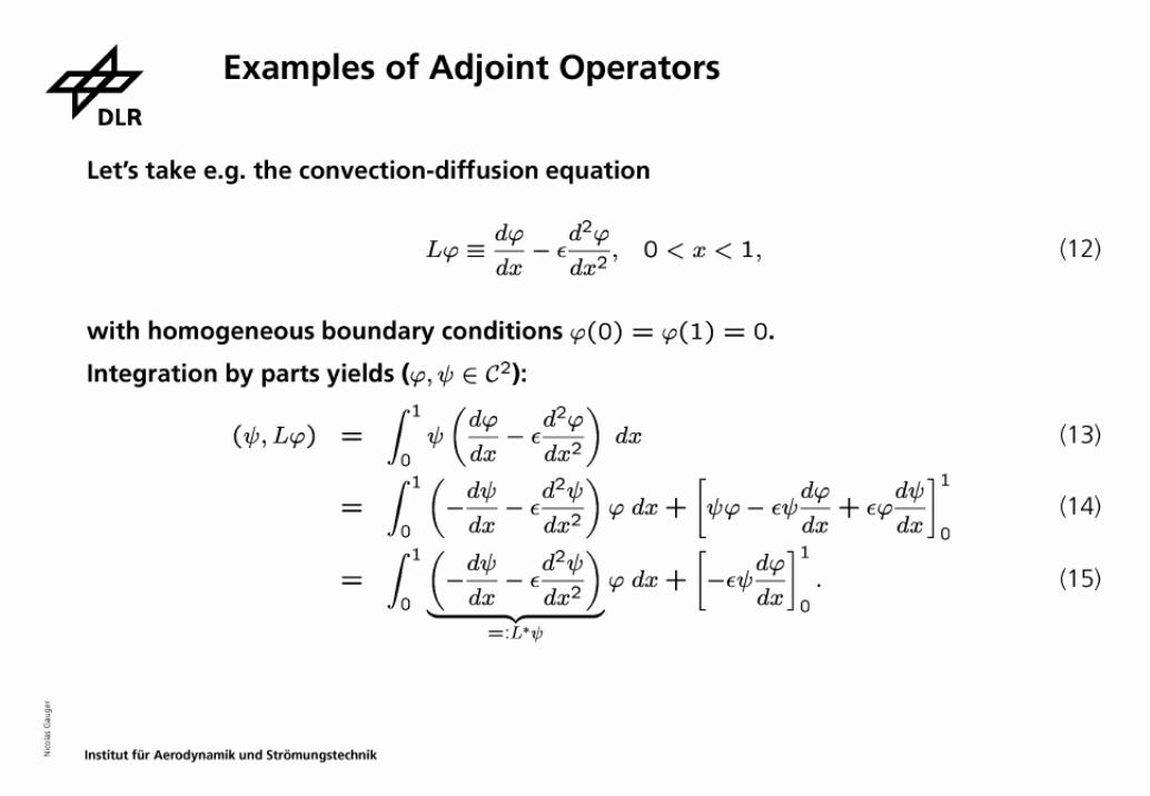
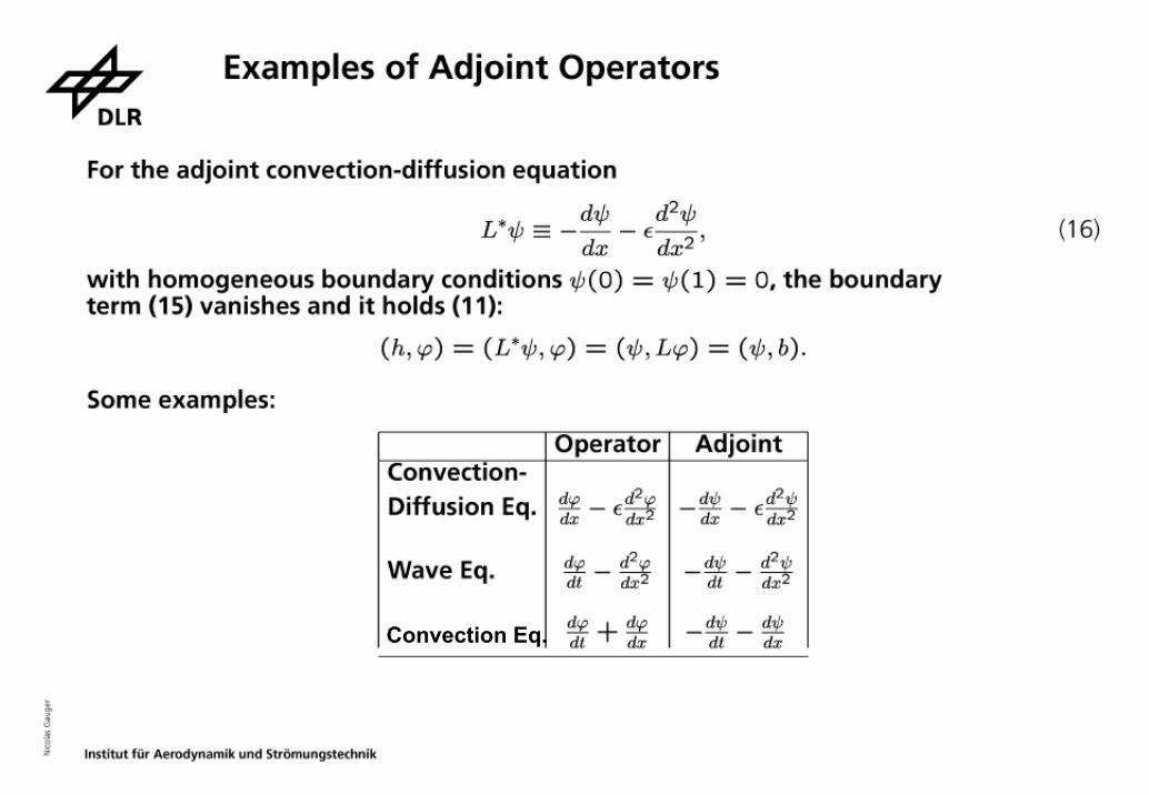
Convection Eq.
23N. Gauger et al.Intro to Optimization and MDO, VKI, March 6-10,2006
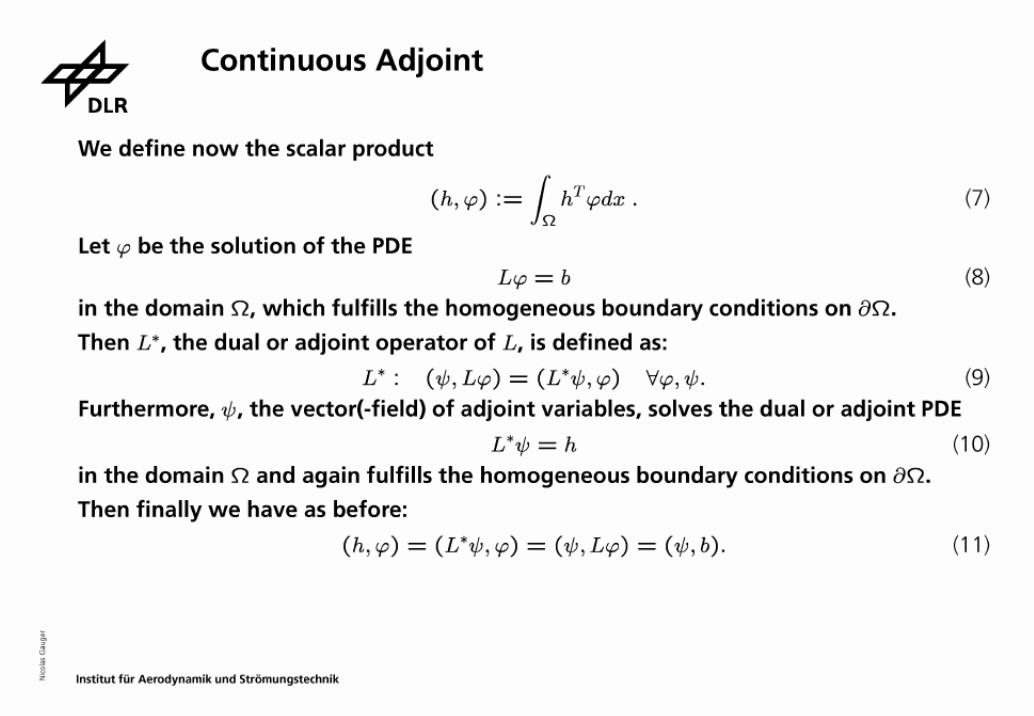
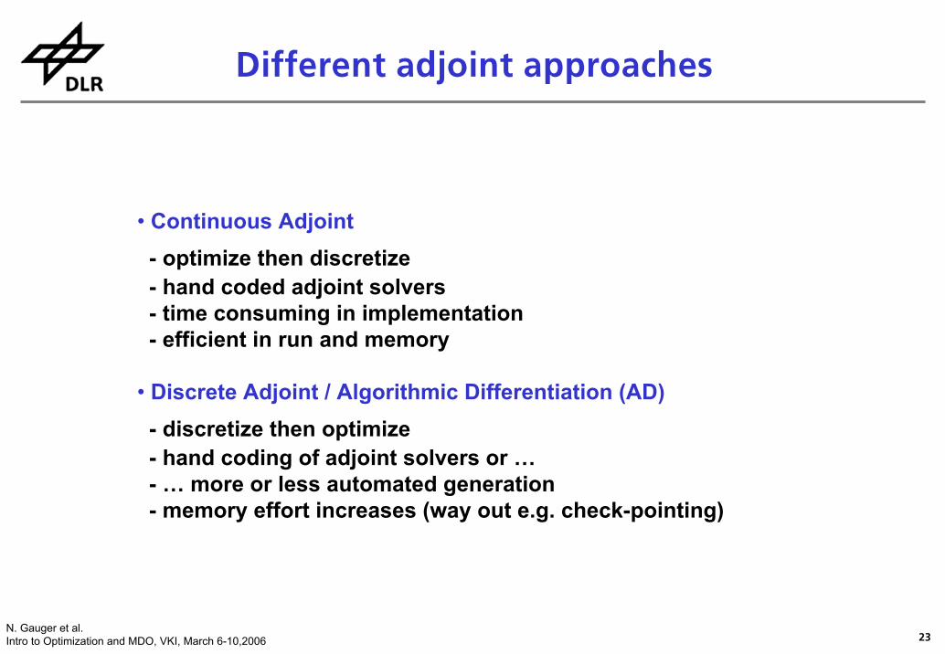
• Continuous Adjoint- optimize then discretize- hand coded adjoint solvers- time consuming in implementation- efficient in run and memory
• Discrete Adjoint / Algorithmic Differentiation (AD)- discretize then optimize- hand coding of adjoint solvers or …- … more or less automated generation- memory effort increases (way out e.g. check-pointing)
Different adjoint approaches
24N. Gauger et al.Intro to Optimization and MDO, VKI, March 6-10,2006
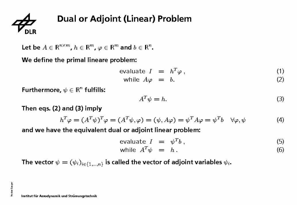
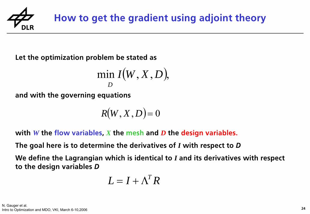
How to get the gradient using adjoint theory
Let the optimization problem be stated as
and with the governing equations
with W the flow variables, X the mesh and D the design variables.
The goal here is to determine the derivatives of I with respect to D
We define the Lagrangian which is identical to I and its derivatives with respect to the design variables D
( ) 0,, =DXWR
( ),,, min D
DXWI
RIL TΛ+=
25N. Gauger et al.Intro to Optimization and MDO, VKI, March 6-10,2006
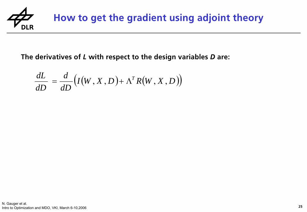
The derivatives of L with respect to the design variables D are:
( ) ( )( )Λ+= DXWRDXWIdDd
dDdL T ,,,,
How to get the gradient using adjoint theory
26N. Gauger et al.Intro to Optimization and MDO, VKI, March 6-10,2006
( ) ( )( )
⎭⎬⎫
⎩⎨⎧
∂∂
+∂∂
+∂∂
Λ+⎭⎬⎫
⎩⎨⎧
∂∂
+∂∂
+∂∂
=
Λ+=
DR
dDdX
XR
dDdW
WRT
DI
dDdX
XI
dDdW
WI
DXWRDXWIdDd
dDdL T
,,,,
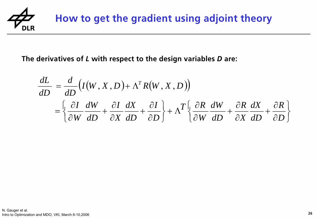
The derivatives of L with respect to the design variables D are:
How to get the gradient using adjoint theory
27N. Gauger et al.Intro to Optimization and MDO, VKI, March 6-10,2006
( ) ( )( )
⎭⎬⎫
⎩⎨⎧
∂∂
Λ+∂∂
+⎭⎬⎫
⎩⎨⎧
∂∂
Λ+∂∂
+⎭⎬⎫
⎩⎨⎧
∂∂
Λ+∂∂
=
⎭⎬⎫
⎩⎨⎧
∂∂
+∂∂
+∂∂
Λ+⎭⎬⎫
⎩⎨⎧
∂∂
+∂∂
+∂∂
=
Λ+=
DRT
DI
dDdX
XRT
XI
dDdW
WRT
WI
DR
dDdX
XR
dDdW
WRT
DI
dDdX
XI
dDdW
WI
DXWRDXWIdDd
dDdL T
,,,,
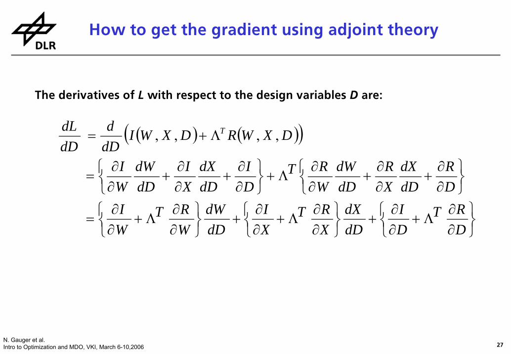
The derivatives of L with respect to the design variables D are:
How to get the gradient using adjoint theory
28N. Gauger et al.Intro to Optimization and MDO, VKI, March 6-10,2006
=0
}
}}
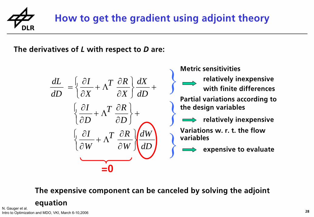
The expensive component can be canceled by solving the adjoint
The derivatives of L with respect to D are:
equation
dDdW
WRT
WI
DRT
DI
dDdX
XRT
XI
dDdL
⎭⎬⎫
⎩⎨⎧
∂∂
Λ+∂∂
+⎭⎬⎫
⎩⎨⎧
∂∂
Λ+∂∂
+⎭⎬⎫
⎩⎨⎧
∂∂
Λ+∂∂
=
Variations w. r. t. the flow variables
expensive to evaluate
Partial variations according to the design variables
relatively inexpensive
Metric sensitivities
relatively inexpensive with finite differences
How to get the gradient using adjoint theory
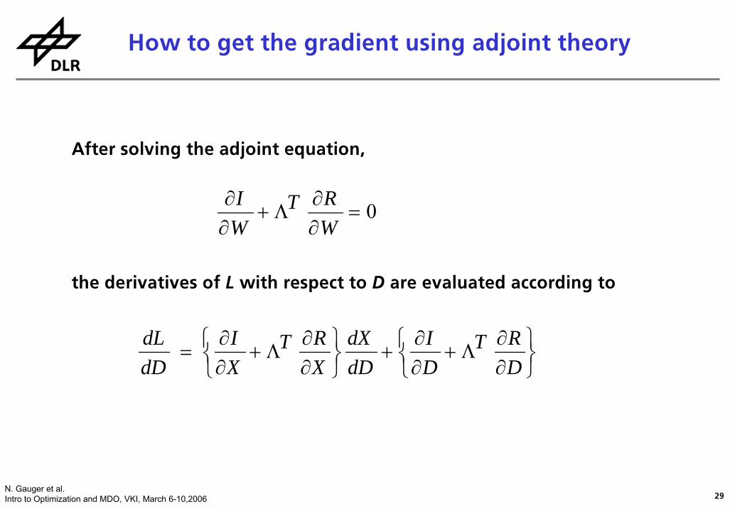
29N. Gauger et al.Intro to Optimization and MDO, VKI, March 6-10,2006
After solving the adjoint equation,
the derivatives of L with respect to D are evaluated according to
⎭⎬⎫
⎩⎨⎧
∂∂
Λ+∂∂
+⎭⎬⎫
⎩⎨⎧
∂∂
Λ+∂∂
=DRT
DI
dDdX
XRT
XI
dDdL
0=∂∂
Λ+∂∂
WRT
WI
How to get the gradient using adjoint theory
30N. Gauger et al.Intro to Optimization and MDO, VKI, March 6-10,2006
31N. Gauger et al.Intro to Optimization and MDO, VKI, March 6-10,2006
32N. Gauger et al.Intro to Optimization and MDO, VKI, March 6-10,2006
33N. Gauger et al.Intro to Optimization and MDO, VKI, March 6-10,2006
34N. Gauger et al.Intro to Optimization and MDO, VKI, March 6-10,2006
35N. Gauger et al.Intro to Optimization and MDO, VKI, March 6-10,2006
36N. Gauger et al.Intro to Optimization and MDO, VKI, March 6-10,2006
37N. Gauger et al.Intro to Optimization and MDO, VKI, March 6-10,2006
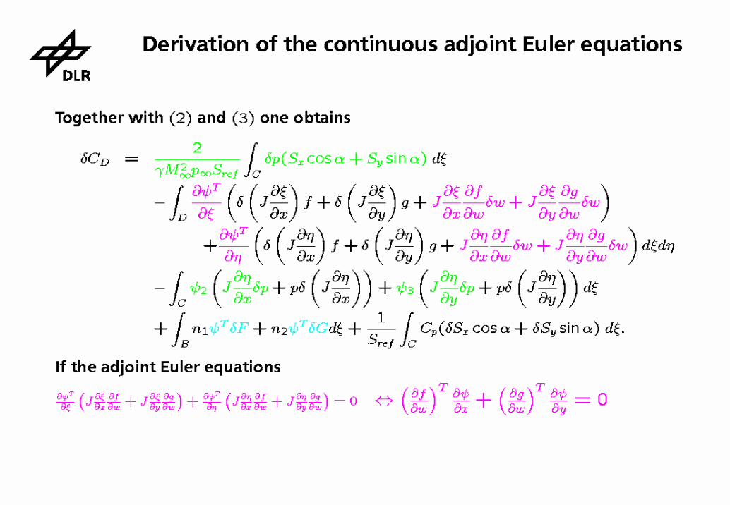
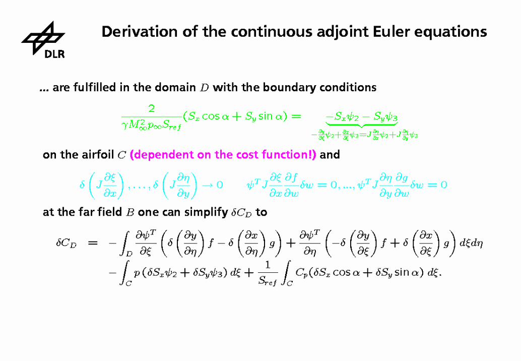
0=∂∂
⎟⎠⎞
⎜⎝⎛
∂∂
−∂∂
⎟⎠⎞
⎜⎝⎛
∂∂
−∂
∂−
ywg
xwf
t
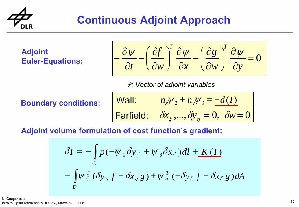
TT ψψψAdjointEuler-Equations:
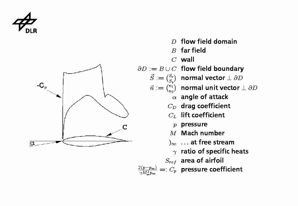
Boundary conditions:
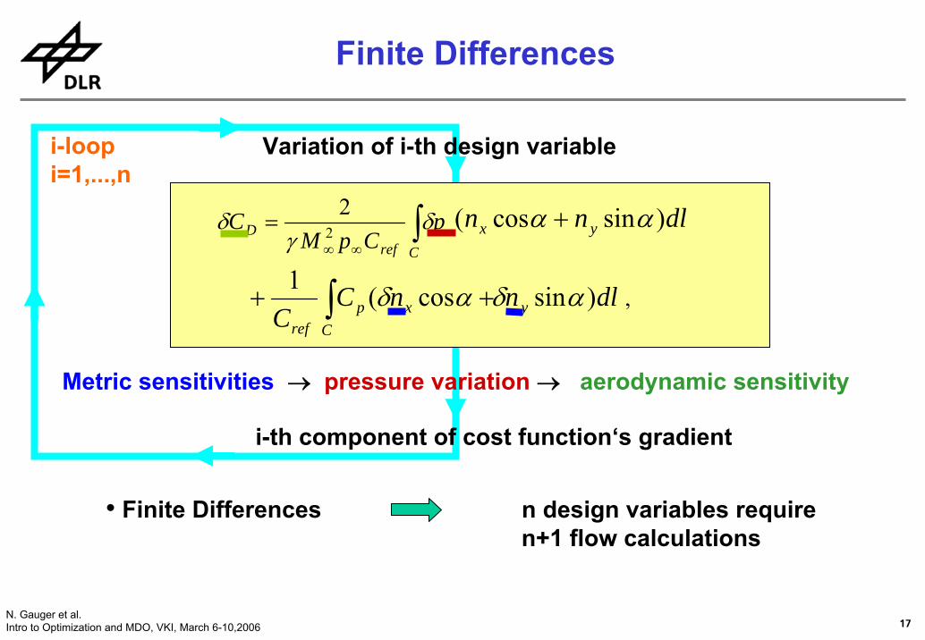
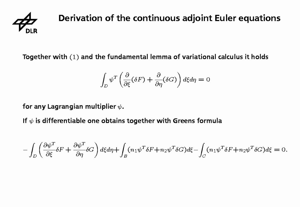
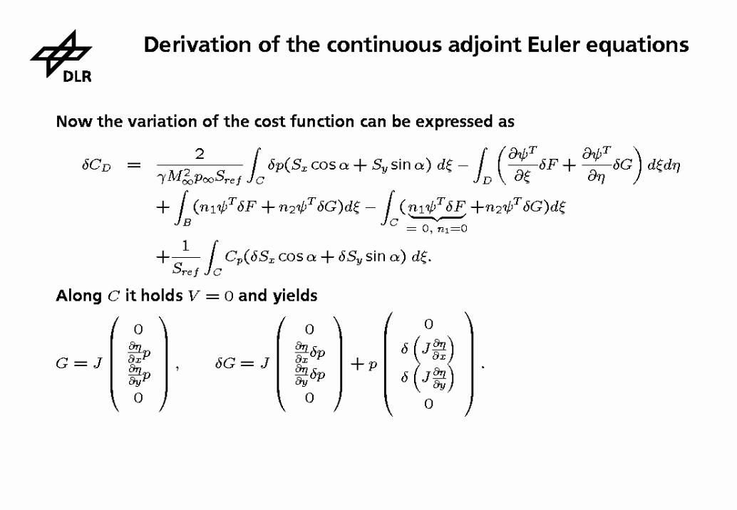
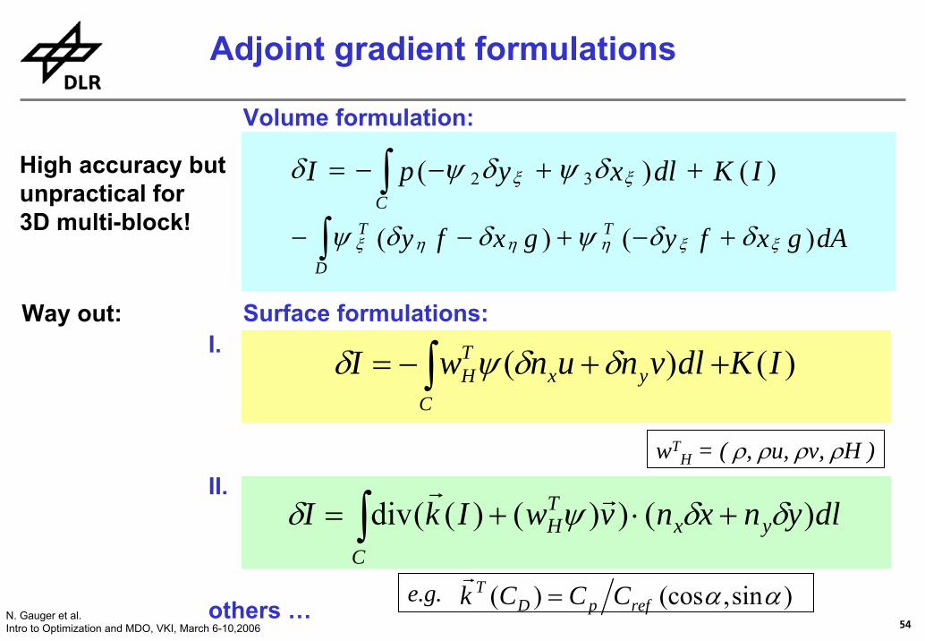
∫ ++−−=C
IKdlxypI )()( 32 ξξ δψδψδ
∫ +−+−−D
TT dAgxfygxfy )()( ξξηηηξ δδψδδψ
Adjoint volume formulation of cost function’s gradient:
Ψ: Vector of adjoint variables
)(32 Idnn yx −=+ ψψ
0=wδ,0,..., =ηξ δδ yxWall:Farfield:
Continuous Adjoint Approach
38N. Gauger et al.Intro to Optimization and MDO, VKI, March 6-10,2006
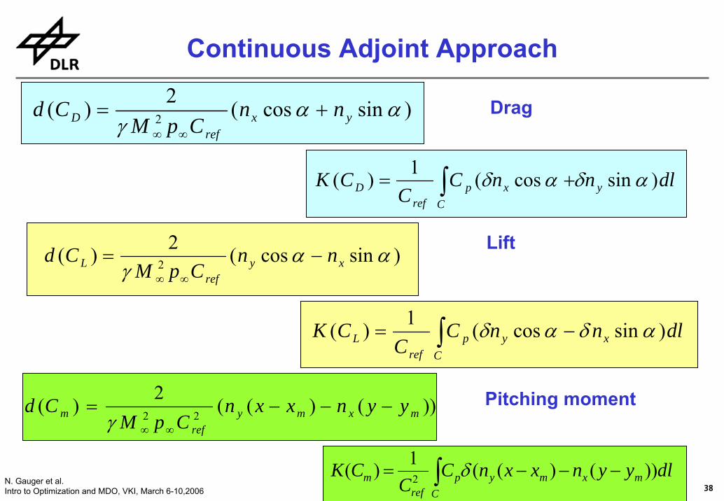
)sincos(2)( 2 ααγ yx
refD nn
CpMCd +=
∞∞
dlnnCC
CK yC
xpref
D )sincos(1)( αδαδ∫ +=
)sincos(2)( 2 ααγ xy
refL nn
CpMCd −=
∞∞
dlnnCC
CK xC
ypref
L )sincos(1)( αδαδ∫ −=
))()((2
)(22 mxmyref
m yynxxnCpM
Cd −−−=∞∞γ
dlyynxxnCC
CKC
mxmypref
m ))()((1)( 2 ∫ −−−= δ
Drag
Pitching moment
Lift
Continuous Adjoint Approach
39N. Gauger et al.Intro to Optimization and MDO, VKI, March 6-10,2006
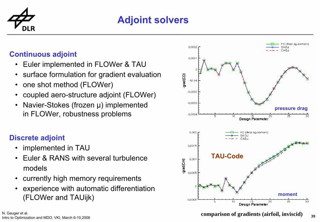
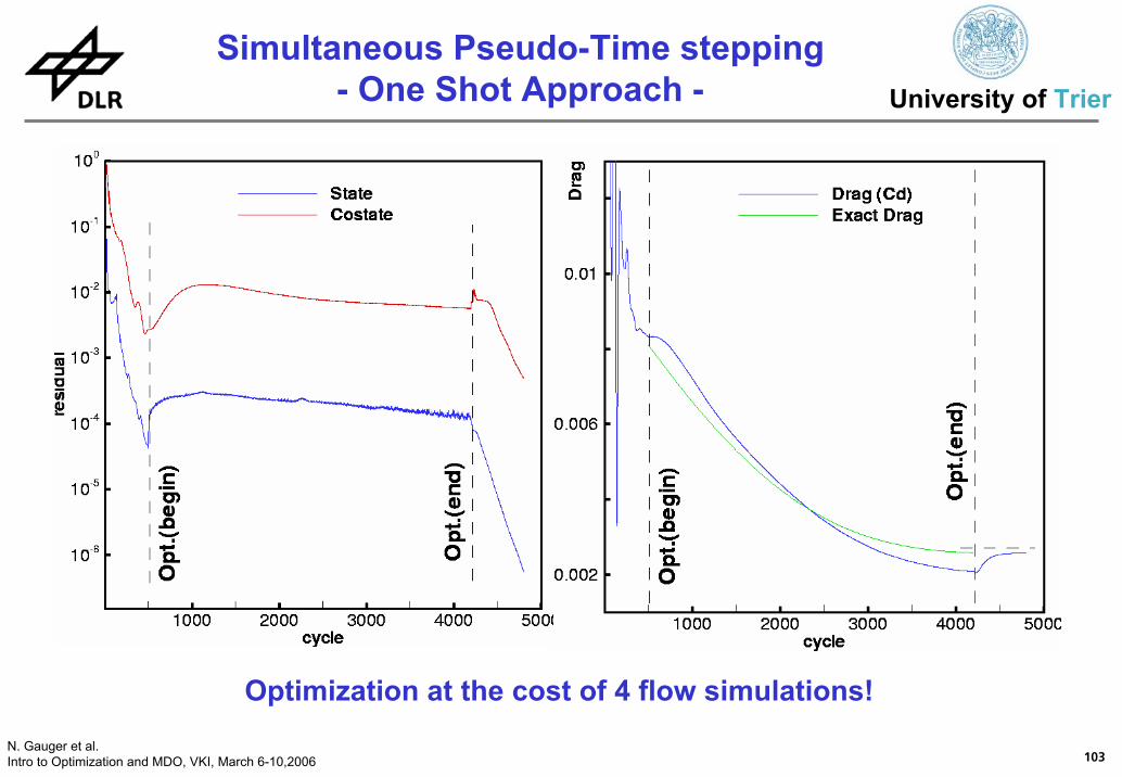
Continuous adjoint• Euler implemented in FLOWer & TAU• surface formulation for gradient evaluation• one shot method (FLOWer)• coupled aero-structure adjoint (FLOWer) • Navier-Stokes (frozen μ) implemented
in FLOWer, robustness problems
Discrete adjoint• implemented in TAU • Euler & RANS with several turbulence
models• currently high memory requirements• experience with automatic differentiation
(FLOWer and TAUijk) moment
pressure drag
TAU-Code
comparison of gradients (airfoil, inviscid)
Adjoint solvers
40N. Gauger et al.Intro to Optimization and MDO, VKI, March 6-10,2006
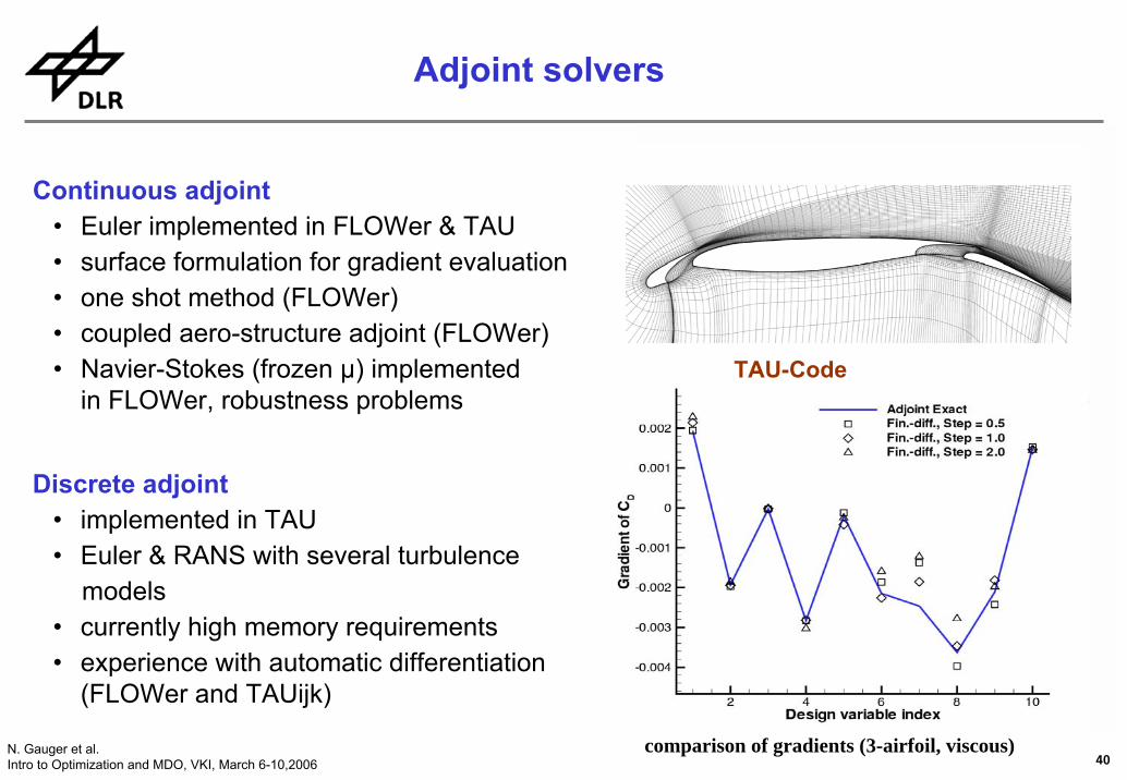
Continuous adjoint• Euler implemented in FLOWer & TAU• surface formulation for gradient evaluation• one shot method (FLOWer)• coupled aero-structure adjoint (FLOWer) • Navier-Stokes (frozen μ) implemented
in FLOWer, robustness problems
Discrete adjoint• implemented in TAU • Euler & RANS with several turbulence
models• currently high memory requirements• experience with automatic differentiation
(FLOWer and TAUijk) moment
pressure drag
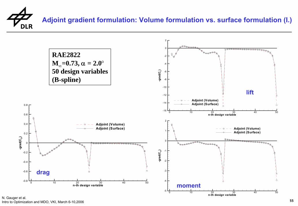
comparison of gradients (airfoil, inviscid)
TAU-Code
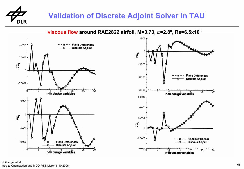
comparison of gradients (3-airfoil, viscous)
TAU-Code
Adjoint solvers
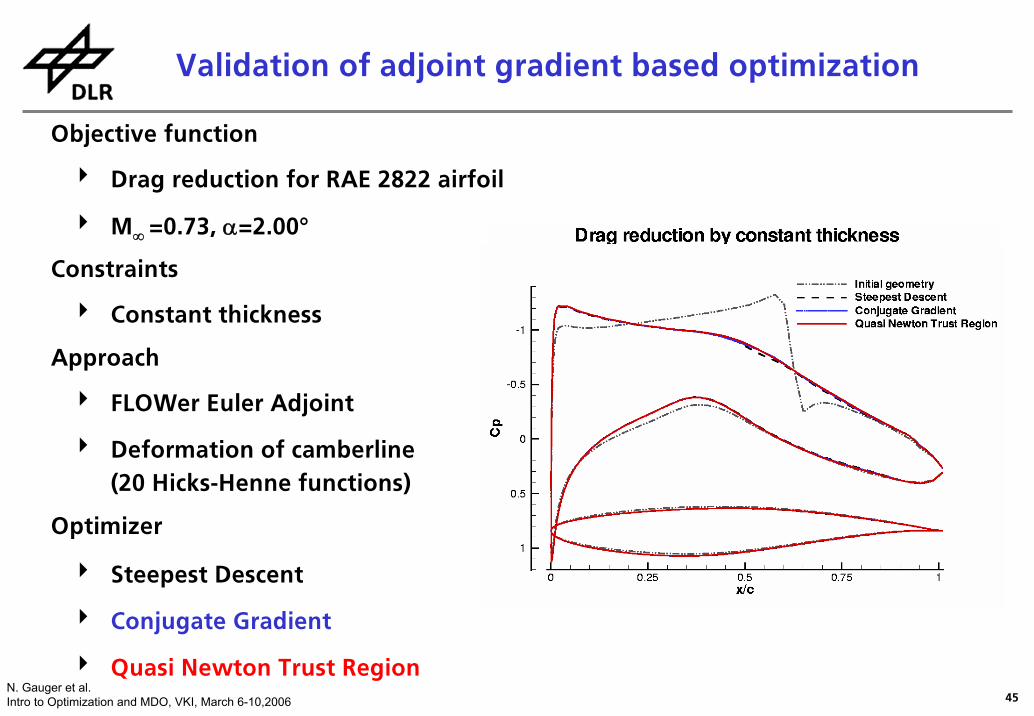
41N. Gauger et al.Intro to Optimization and MDO, VKI, March 6-10,2006
flowsolution
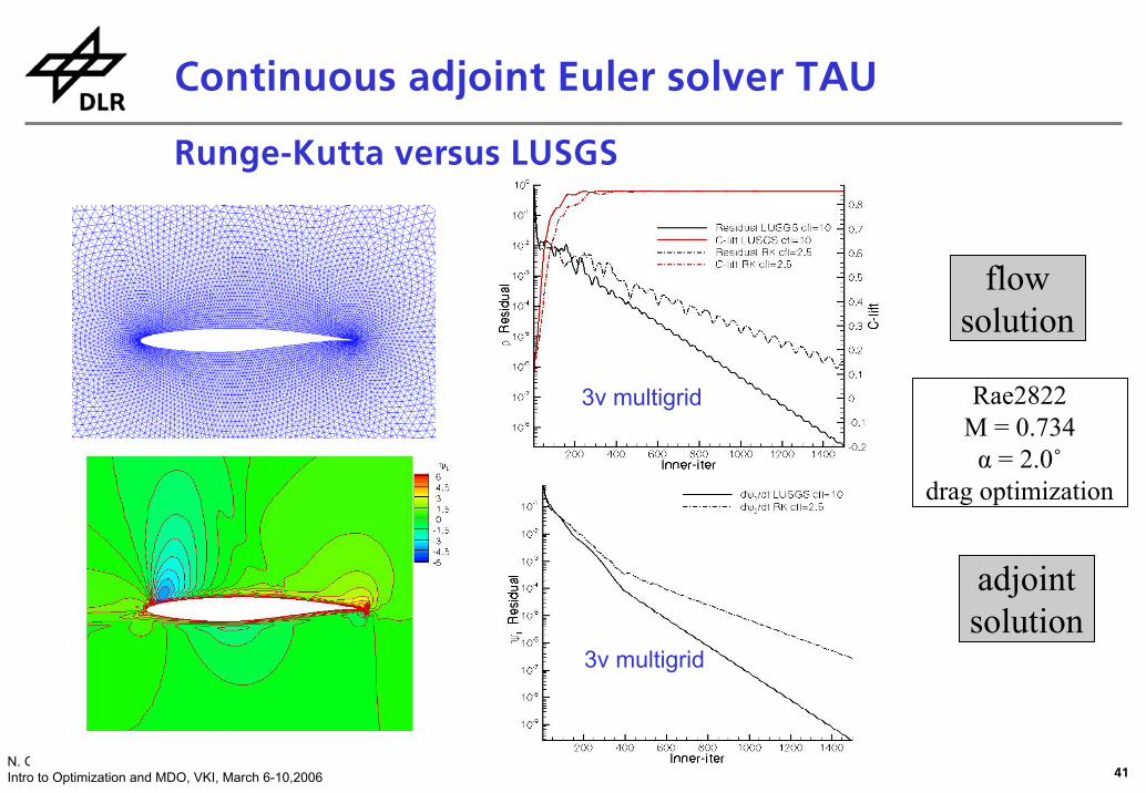
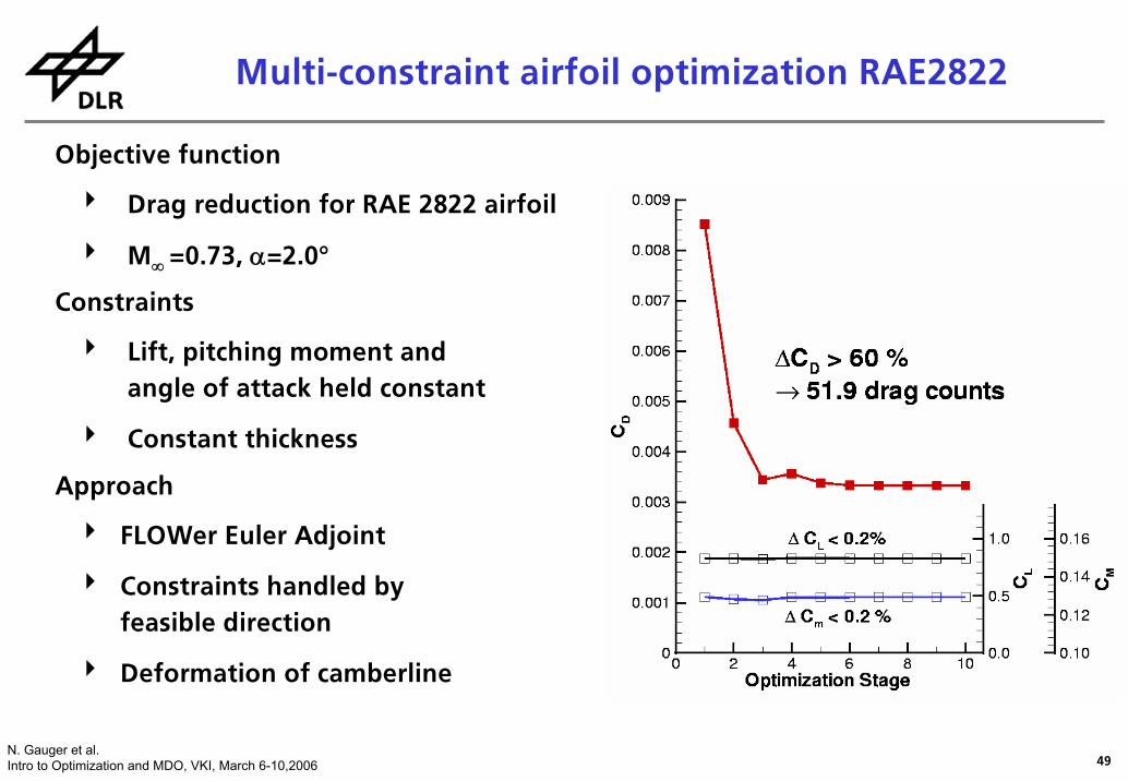
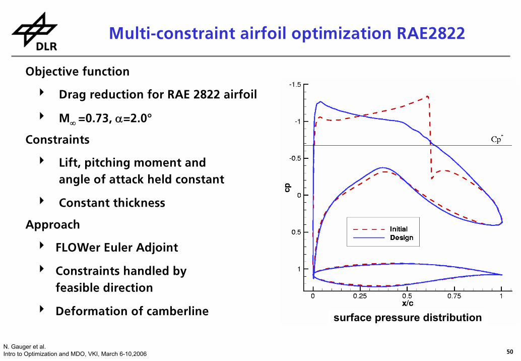
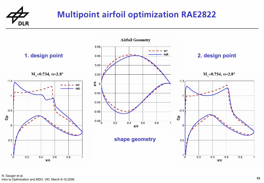
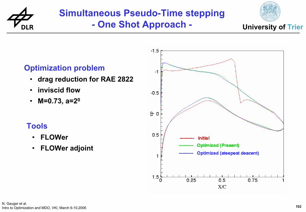
Rae2822M = 0.734α = 2.0˚
drag optimization
adjointsolution
3v multigrid
3v multigrid
Continuous adjoint Euler solver TAU
Runge-Kutta versus LUSGS
42N. Gauger et al.Intro to Optimization and MDO, VKI, March 6-10,2006
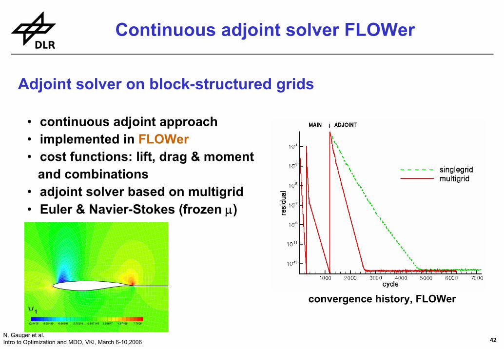
Continuous adjoint solver FLOWer
Adjoint solver on block-structured grids
• continuous adjoint approach• implemented in FLOWer• cost functions: lift, drag & moment
and combinations • adjoint solver based on multigrid• Euler & Navier-Stokes (frozen μ)
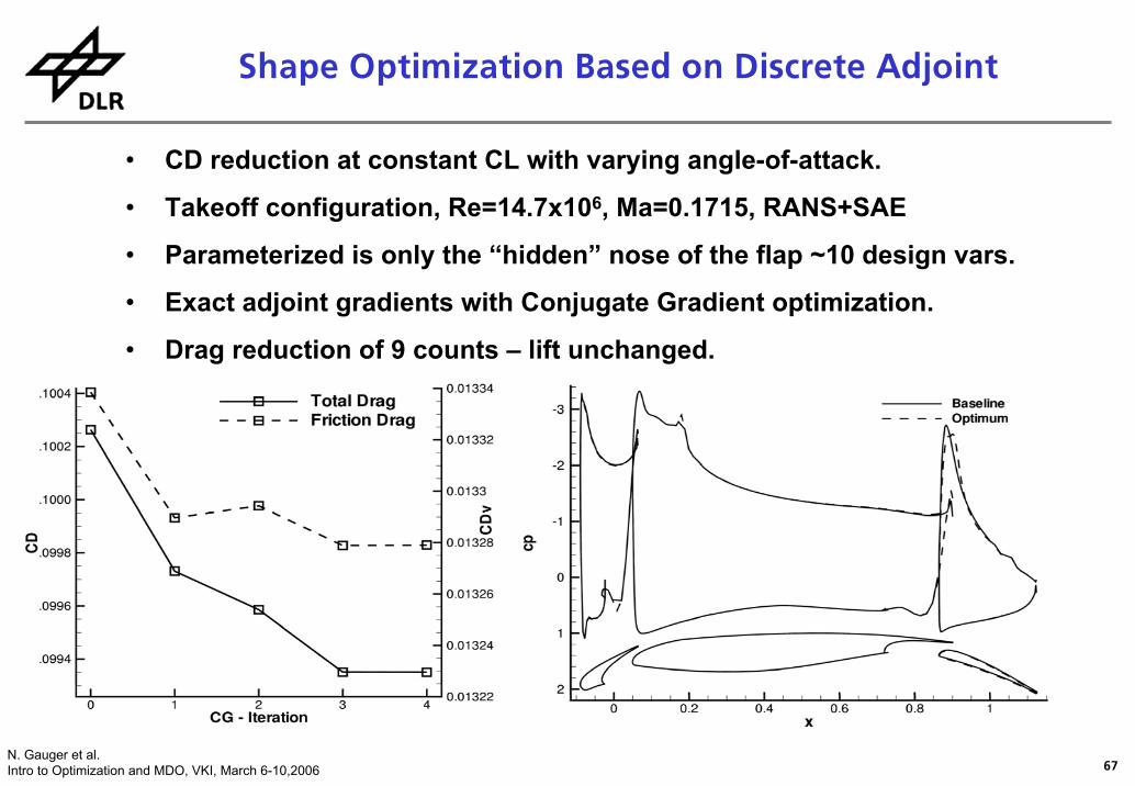
• Parameterized is only the “hidden” nose of the flap ~10 design vars.
• Exact adjoint gradients with Conjugate Gradient optimization.
• Drag reduction of 9 counts – lift unchanged.
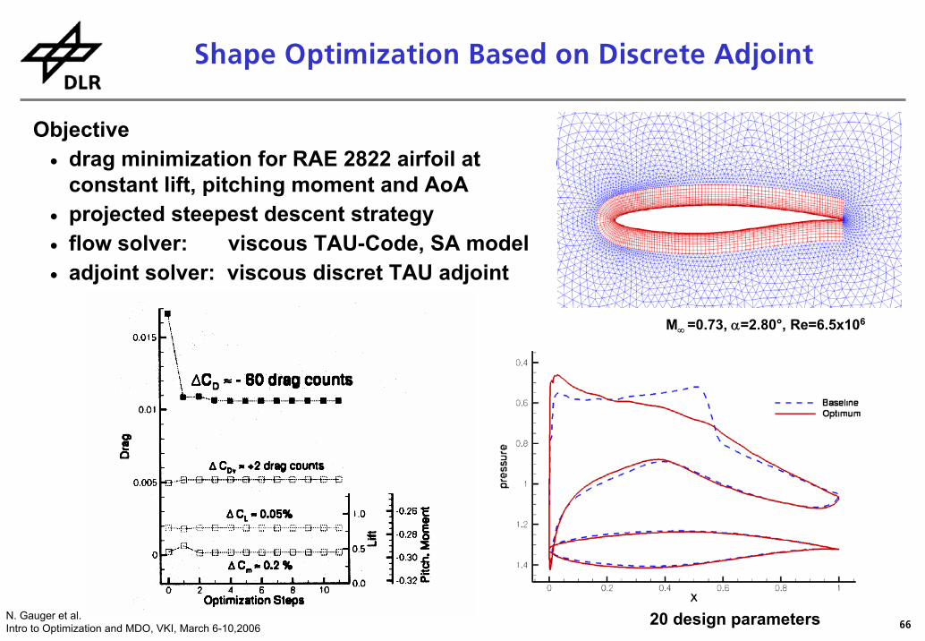
Shape Optimization Based on Discrete Adjoint
68N. Gauger et al.Intro to Optimization and MDO, VKI, March 6-10,2006
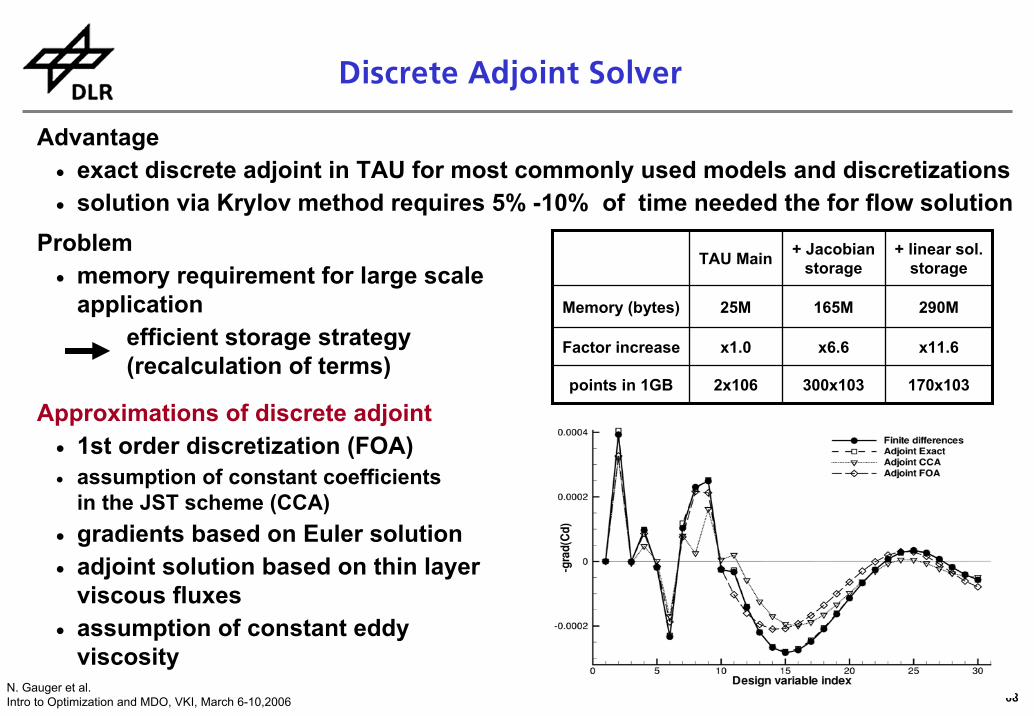
Discrete Adjoint Solver
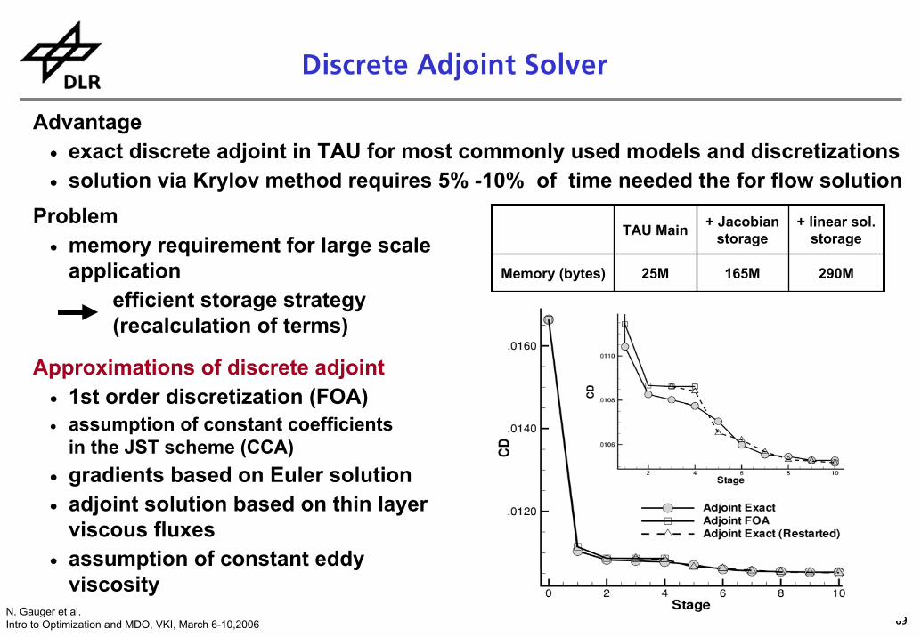
Advantage• exact discrete adjoint in TAU for most commonly used models and discretizations• solution via Krylov method requires 5% -10% of time needed the for flow solution
Problem• memory requirement for large scale
application efficient storage strategy(recalculation of terms)
TAU Main + Jacobianstorage
+ linear sol.storage
Memory (bytes) 25M 165M 290M
Factor increase x1.0 x6.6 x11.6
points in 1GB 2x10⁶ 300x103 170x103
Approximations of discrete adjoint• 1st order discretization (FOA)• assumption of constant coefficients
in the JST scheme (CCA)• gradients based on Euler solution• adjoint solution based on thin layer
viscous fluxes• assumption of constant eddy
viscosity
Discrete Adjoint Solver
69N. Gauger et al.Intro to Optimization and MDO, VKI, March 6-10,2006
Discrete Adjoint Solver
Advantage• exact discrete adjoint in TAU for most commonly used models and discretizations• solution via Krylov method requires 5% -10% of time needed the for flow solution
Problem• memory requirement for large scale
application efficient storage strategy(recalculation of terms)
TAU Main + Jacobianstorage
+ linear sol.storage
Memory (bytes) 25M 165M 290M
Factor increase x1.0 x6.6 x11.6
points in 1GB 2x10⁶ 300x103 170x103
Approximations of discrete adjoint• 1st order discretization (FOA)• assumption of constant coefficients
in the JST scheme (CCA)• gradients based on Euler solution• adjoint solution based on thin layer
viscous fluxes• assumption of constant eddy
viscosity
Discrete Adjoint Solver
70N. Gauger et al.Intro to Optimization and MDO, VKI, March 6-10,2006
Algorithmic Differentiation (AD)
Work in progress and results
• ADFLOWer generated with TAF (3D Navier-Stokes,k-w), first verifications and validation
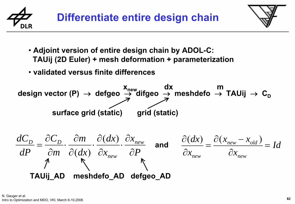
• Adjoint version of TAUij (2D Euler) + mesh deformationand parameterization with ADOL-C, validated versus finite differences and first applications
• First and second derivatives of a “FLOWer-Derivate”(2D Euler) + mesh deformation and parameterizationgenerated with TAPENADE, used for One Shot (Piggy Back)
71N. Gauger et al.Intro to Optimization and MDO, VKI, March 6-10,2006
72N. Gauger et al.Intro to Optimization and MDO, VKI, March 6-10,2006
73N. Gauger et al.Intro to Optimization and MDO, VKI, March 6-10,2006
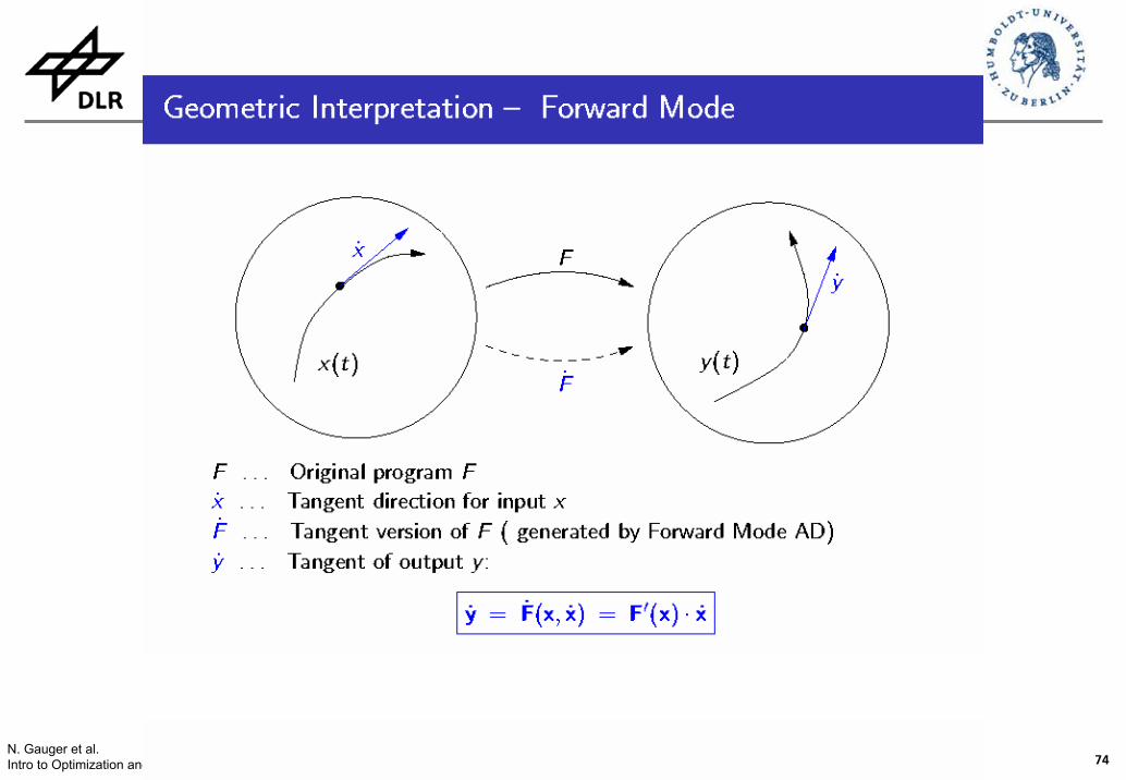
Evaluation of Simple Example:
Simple Example
74N. Gauger et al.Intro to Optimization and MDO, VKI, March 6-10,2006
75N. Gauger et al.Intro to Optimization and MDO, VKI, March 6-10,2006
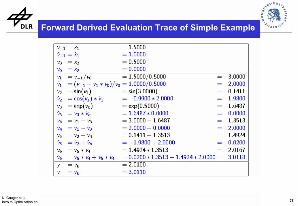
Forward Derived Evaluation Trace of Simple Example
76N. Gauger et al.Intro to Optimization and MDO, VKI, March 6-10,2006
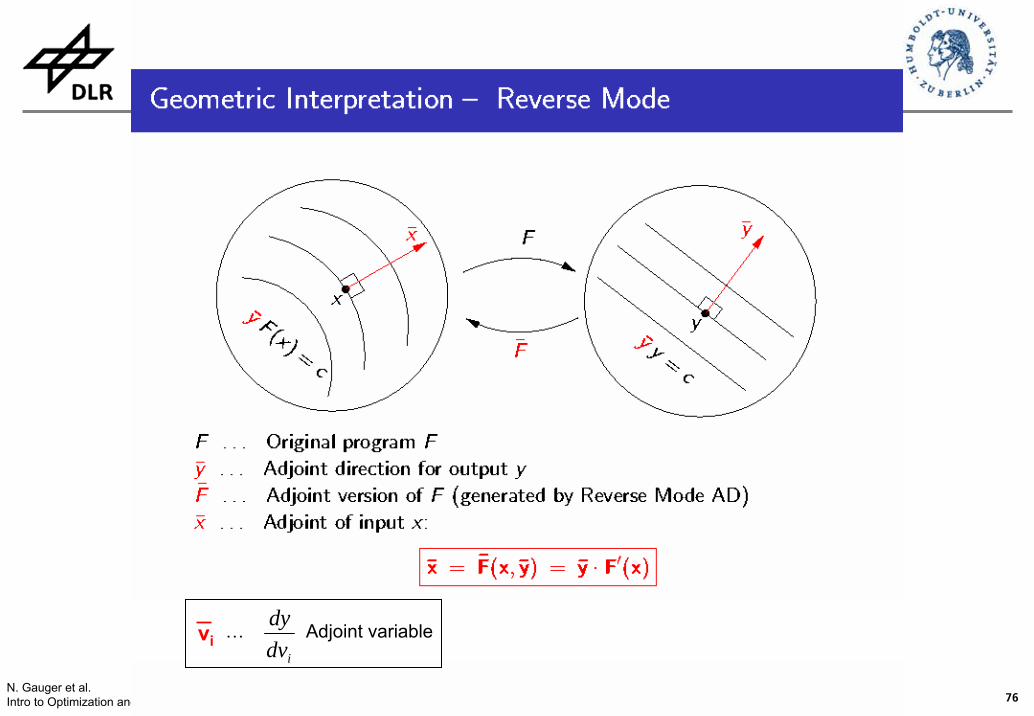
idvdy
vi … Adjoint variable
77N. Gauger et al.Intro to Optimization and MDO, VKI, March 6-10,2006
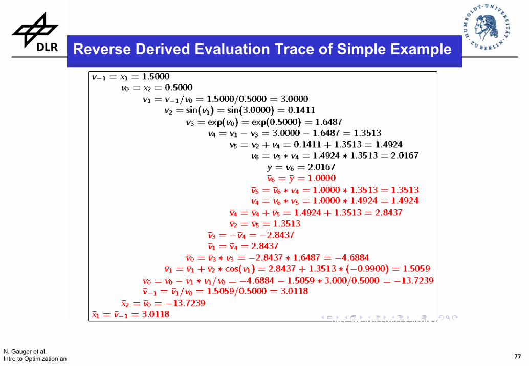
Reverse Derived Evaluation Trace of Simple Example
78N. Gauger et al.Intro to Optimization and MDO, VKI, March 6-10,2006
FastOpt
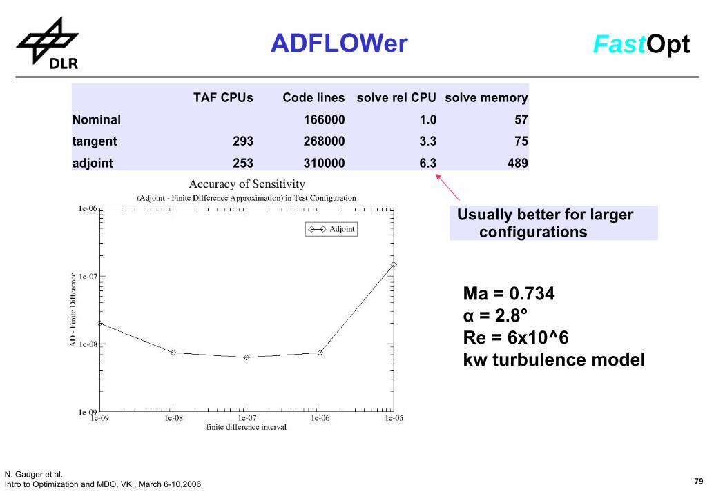
Test configuration2d NACA12k-omega (Wilcox) turbulence modelcell-centred metric2 time steps on fine gridtarget sensitivity: d lift/ d alpha
StepsModifications of FLOWer code (TAF Directives, slight recoding, etc...)tangent-linear code (verification + useful per se small dimensional design problems) adjoint codeeifficient adjoint code
Major challengememory management (all variables in one big field 'variab')complicates detailed analysis and handling of deallocation
ADFLOWer by TAF
79N. Gauger et al.Intro to Optimization and MDO, VKI, March 6-10,2006
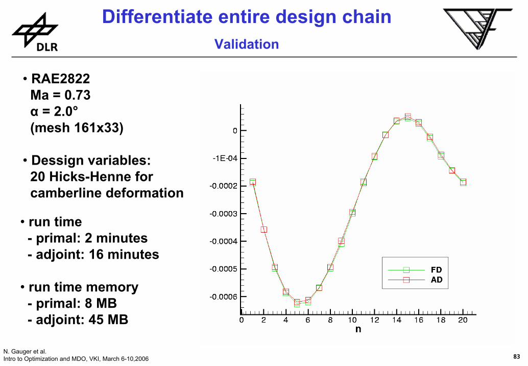
• run time- primal: 2 minutes- adjoint: 16 minutes
• run time memory- primal: 8 MB- adjoint: 45 MB
Differentiate entire design chainValidation
84N. Gauger et al.Intro to Optimization and MDO, VKI, March 6-10,2006
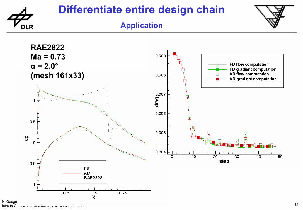
Differentiate entire design chainApplication
RAE2822Ma = 0.73α = 2.0°(mesh 161x33)
85N. Gauger et al.Intro to Optimization and MDO, VKI, March 6-10,2006
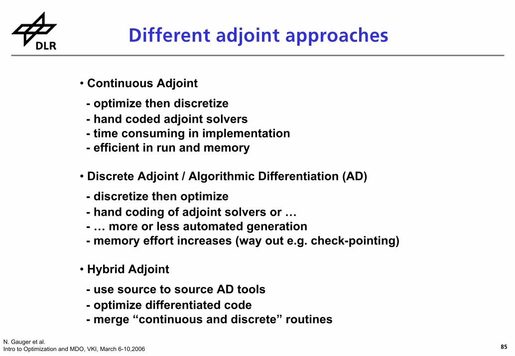
• Continuous Adjoint- optimize then discretize- hand coded adjoint solvers- time consuming in implementation- efficient in run and memory
• Discrete Adjoint / Algorithmic Differentiation (AD)- discretize then optimize- hand coding of adjoint solvers or …- … more or less automated generation- memory effort increases (way out e.g. check-pointing)
• Hybrid Adjoint- use source to source AD tools - optimize differentiated code- merge “continuous and discrete” routines
Different adjoint approaches
86N. Gauger et al.Intro to Optimization and MDO, VKI, March 6-10,2006
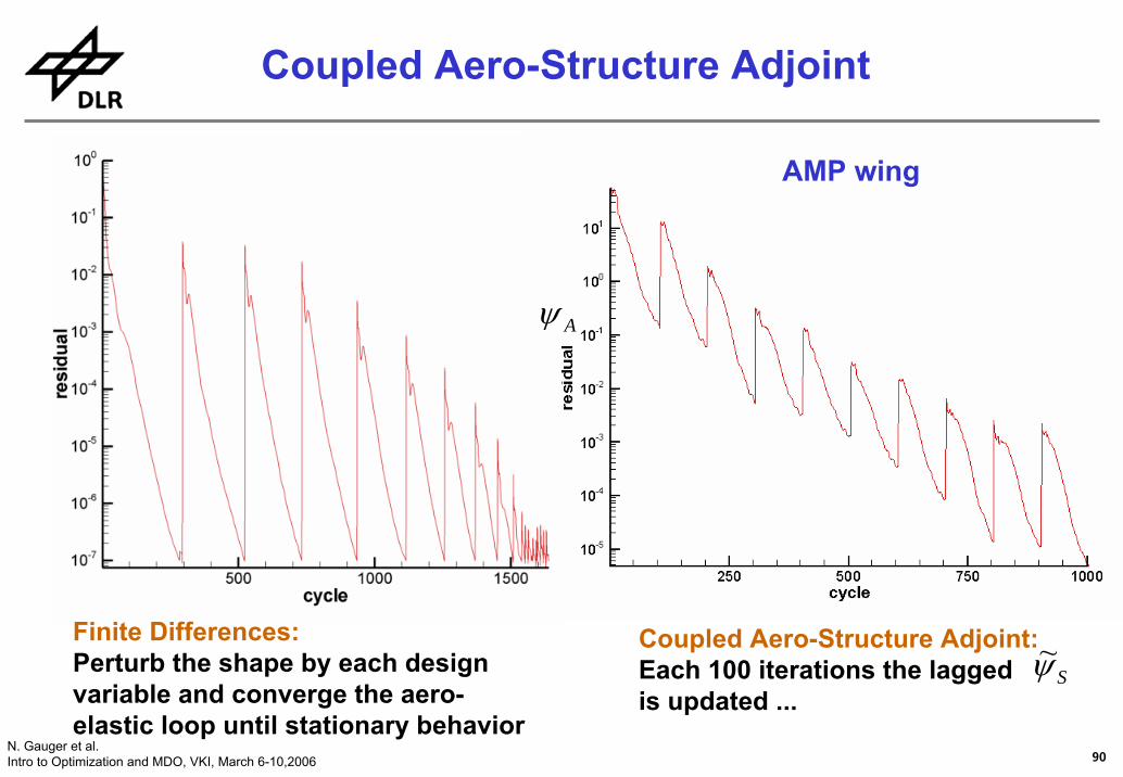
Coupled Aero-Structure Adjoint
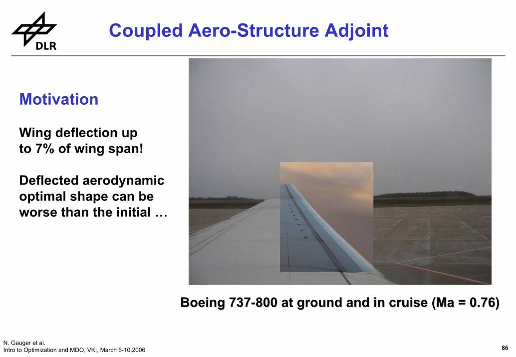
Motivation
Wing deflection up to 7% of wing span!
Deflected aerodynamicoptimal shape can beworse than the initial …
Boeing 737Boeing 737--800 at ground and in cruise (Ma = 0.76)800 at ground and in cruise (Ma = 0.76)
87N. Gauger et al.Intro to Optimization and MDO, VKI, March 6-10,2006
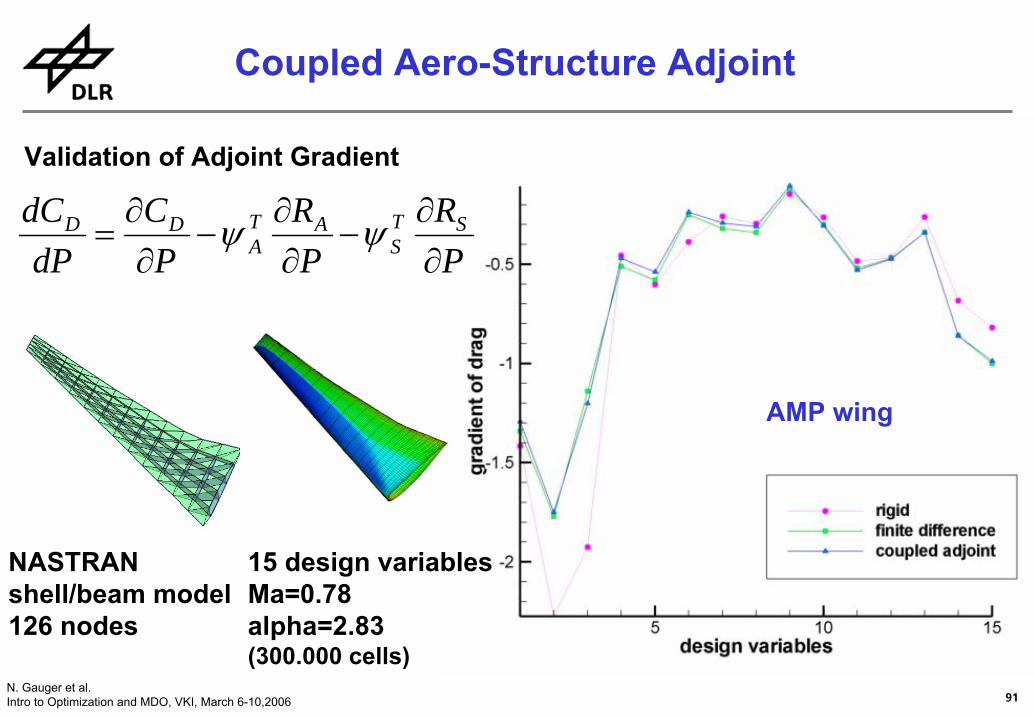
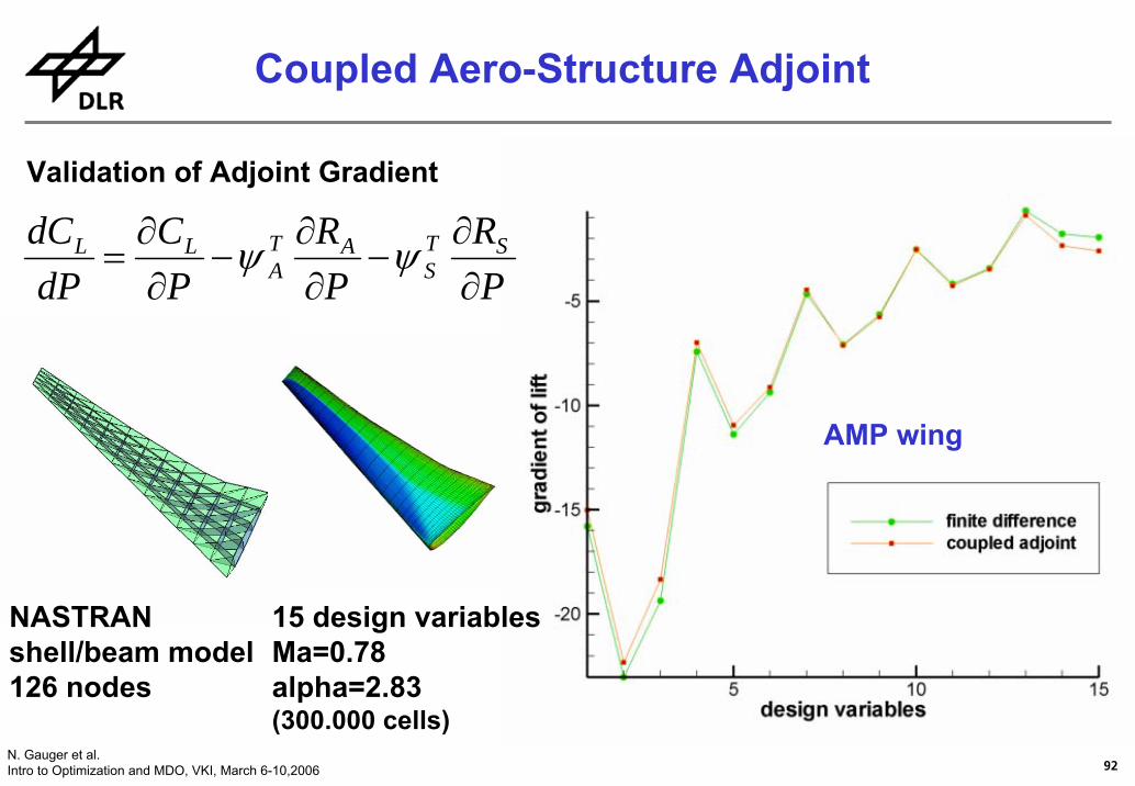
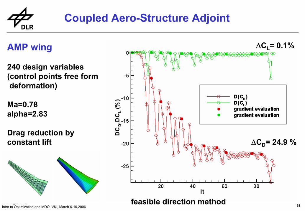
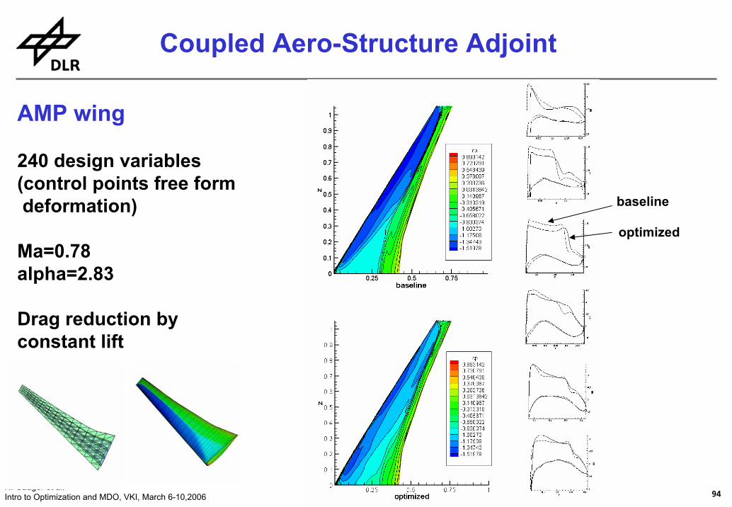
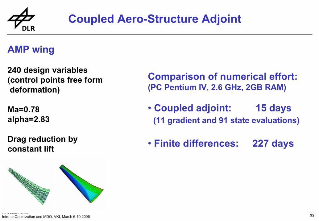
Coupled Aero-Structure Adjoint
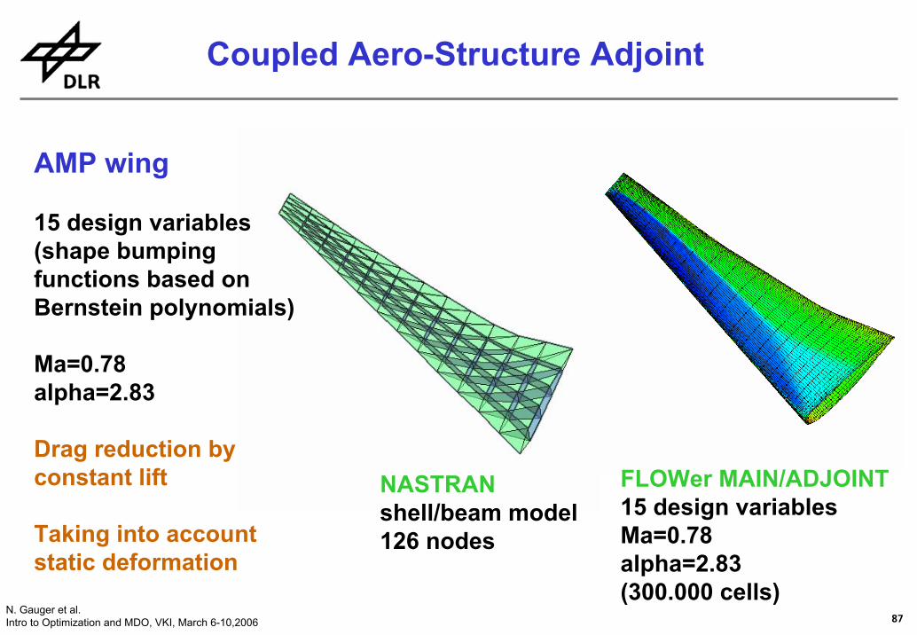
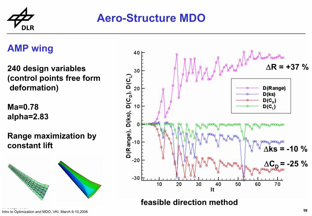
AMP wing
15 design variables(shape bumping functions based on Bernstein polynomials)