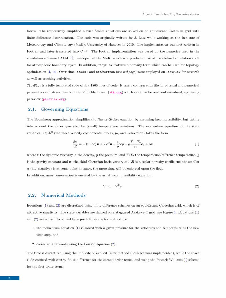
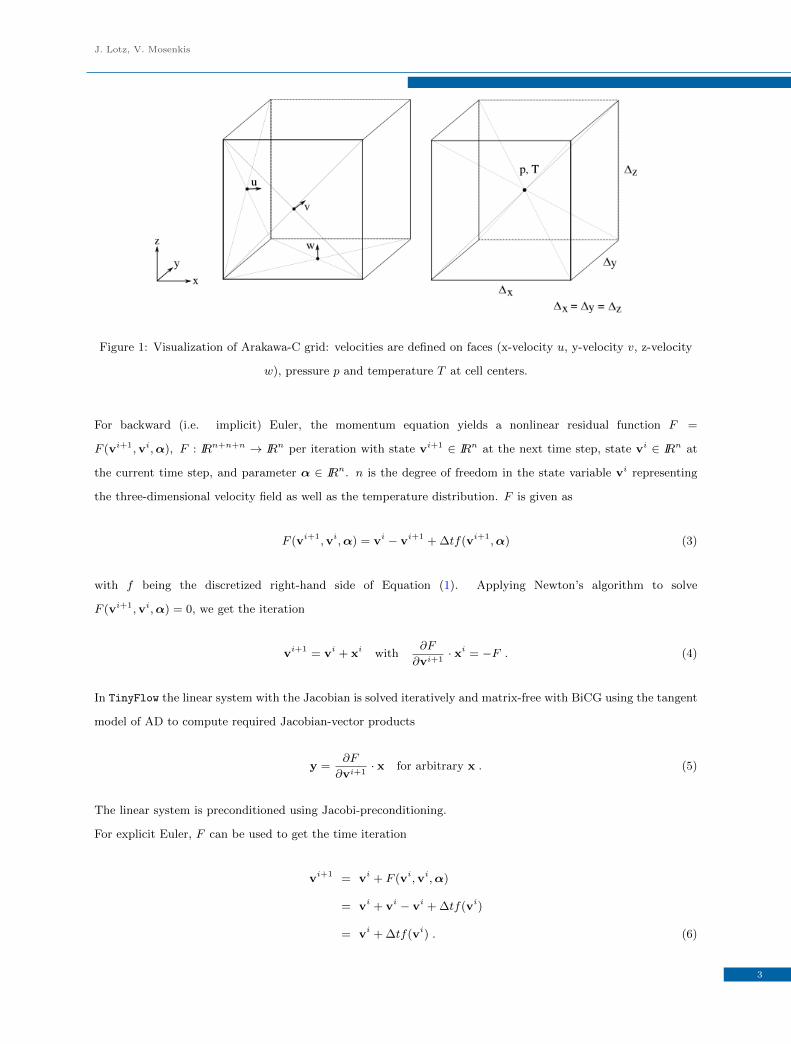
+ All Categories
Home > Documents > Adjoint Flow Solver TinyFlow using dco/c++ · Equations (1) and (2) are discretized using nite di...

Adjoint Flow Solver TinyFlow using dco/c++ · Equations (1) and (2) are discretized using nite di...

Date post: 14-Mar-2020
Category:
Upload: others
View: 12 times
Download: 2 times
Share this document with a friend
16
Tech.Rep. 1-16 Author version Technical Report Adjoint Flow Solver TinyFlow using dco/c ++ Johannes Lotz 1* and Viktor Mosenkis 2 1 Software and Tools for Computational Engineering 2 Numerical Algorithms Group Abstract: Adjoints of large numerical solvers are used more and in industry and academia, e.g. in computational fluid dynamics, finance and engineering. Using algorithmic differentiation is a convenient and efficient of generat- ing adjoint codes automatically from a given primal. This document reports the application of algorithmic differentiation using dco/c++ to a demonstrator flow solver, which makes use of various NAG Library routines. Since the NAG Library supports dco/c++ data types, seamless integration is possible (as shown in this report). Simple switches between algorithmic and symbolic versions of the NAG routines can be used to minimize memory usage. Keywords: NAG Library Adjoints Algorithmic Differentiation dco/c++ CFD c Numerical Algorithms Group Ltd. 1. Introduction This technical report serves as a demonstrator on how to use dco/c++ and the NAG AD Library to compute adjoints of a non-trivial PDE (partial differential equation) solver. It shows how dco/c++ can be used to couple hand-written symbolic adjoint code with an overall algorithmic solution; but it also demonstrates the easy-to-use interface when dco/c++ is coupled with the NAG AD Library (nag.co.uk/content/adjoint-algorithmic-differentiation referred to as webpage in the following). Here, the sparse linear solver f11jc can be switched from algorithmic to symbolic mode in one code line. The next section introduces the primal solver followed by sections about the adjoint solver and respective run time and memory results. Also, an optimization algorithm is run on a test case using steepest descent to show potential use of the computed adjoints. 2. Primal Solver TinyFlow is a non-validated three-dimensional unsteady incompressible DNS (direct numerical simulation, i.e. no turbulence model) solver with Boussinesq approximation [1, 2] for modeling temperature dependency on vertical * E-mail: [email protected] 1
Transcript

Tech.Rep. • 1-16Author version

Technical Report

Adjoint Flow Solver TinyFlow using dco/c++

Johannes Lotz1∗ and Viktor Mosenkis2

1 Software and Tools for Computational Engineering

2 Numerical Algorithms Group

Abstract: Adjoints of large numerical solvers are used more and in industry and academia, e.g. in computational fluid

dynamics, finance and engineering. Using algorithmic differentiation is a convenient and efficient of generat-

ing adjoint codes automatically from a given primal. This document reports the application of algorithmicdifferentiation using dco/c++ to a demonstrator flow solver, which makes use of various NAG Library routines.

Since the NAG Library supports dco/c++ data types, seamless integration is possible (as shown in this report).

Simple switches between algorithmic and symbolic versions of the NAG routines can be used to minimizememory usage.

Keywords: NAG Library • Adjoints • Algorithmic Differentiation • dco/c++ • CFD

c© Numerical Algorithms Group Ltd.

1. Introduction

This technical report serves as a demonstrator on how to use dco/c++ and the NAG AD Library to compute adjoints

of a non-trivial PDE (partial differential equation) solver. It shows how dco/c++ can be used to couple hand-written

symbolic adjoint code with an overall algorithmic solution; but it also demonstrates the easy-to-use interface when

dco/c++ is coupled with the NAG AD Library (nag.co.uk/content/adjoint-algorithmic-differentiation –

referred to as webpage in the following). Here, the sparse linear solver f11jc can be switched from algorithmic to

symbolic mode in one code line.

The next section introduces the primal solver followed by sections about the adjoint solver and respective run

time and memory results. Also, an optimization algorithm is run on a test case using steepest descent to show

potential use of the computed adjoints.

2. Primal Solver

TinyFlow is a non-validated three-dimensional unsteady incompressible DNS (direct numerical simulation, i.e. no

turbulence model) solver with Boussinesq approximation [1, 2] for modeling temperature dependency on vertical

∗ E-mail: [email protected]

1

Adjoint Flow Solver TinyFlow using dco/c++

forces. The respectively simplified Navier–Stokes equations are solved on an equidistant Cartesian grid with

finite difference discretization. The code was originally written by J. Lotz while working at the Institute of

Meteorology and Climatology (MuK), University of Hanover in 2010. The implementation was first written in

Fortran and later translated into C++. The Fortran implementation was based on the numerics used in the

simulation software PALM [3], developed at the MuK, which is a production sized parallelized simulation code

for atmospheric boundary layers. In addition, TinyFlow features a porosity term which can be used for topology

optimization [4, 14]. Over time, dco/c++ and dco/fortran (see webpage) were employed on TinyFlow for research

as well as teaching activities.

TinyFlow is a fully templated code with ∼1800 lines-of-code. It uses a configuration file for physical and numerical

parameters and stores results in the VTK file format (vtk.org) which can then be read and visualized, e.g., using

paraview (paraview.org).

2.1. Governing Equations

The Boussinesq approximation simplifies the Navier–Stokes equation by assuming incompressibility, but taking

into account the forces generated by (small) temperature variations. The momentum equation for the state

variables u ∈ IR3 (the three velocity components into x-, y-, and z-direction) takes the form

du

dt= − (u · ∇)u + ν∇2u− 1

ρ∇p− g T − T0

T0e3 + αu (1)

where ν the dynamic viscosity, ρ the density, p the pressure, and T/T0 the temperature/reference temperature. g

is the gravity constant and e3 the third Cartesian basis vector. α ∈ IR is a scalar porosity coefficient; the smaller

α (i.e. negative) is at some point in space, the more drag will be enforced upon the flow.

In addition, mass conservation is ensured by the usual incompressibility equation

∇ · u = ∇2p . (2)

2.2. Numerical Methods

Equations (1) and (2) are discretized using finite difference schemes on an equidistant Cartesian grid, which is of

attractive simplicity. The state variables are defined on a staggered Arakawa-C grid, see Figure 1. Equations (1)

and (2) are solved decoupled by a predictor-corrector method, i.e.

1. the momentum equation (1) is solved with a given pressure for the velocities and temperature at the new

time step, and

2. corrected afterwards using the Poisson equation (2).

The time is discretized using the implicite or explicit Euler method (both schemes implemented), while the space

is descretized with central finite difference for the second-order terms, and using the Piascek-Williams [9] scheme

for the first-order terms.

2

J. Lotz, V. Mosenkis

Figure 1: Visualization of Arakawa-C grid: velocities are defined on faces (x-velocity u, y-velocity v, z-velocity

w), pressure p and temperature T at cell centers.

For backward (i.e. implicit) Euler, the momentum equation yields a nonlinear residual function F =

F (vi+1,vi,α), F : IRn+n+n → IRn per iteration with state vi+1 ∈ IRn at the next time step, state vi ∈ IRn at

the current time step, and parameter α ∈ IRn. n is the degree of freedom in the state variable vi representing

the three-dimensional velocity field as well as the temperature distribution. F is given as

F (vi+1,vi,α) = vi − vi+1 + ∆tf(vi+1,α) (3)

with f being the discretized right-hand side of Equation (1). Applying Newton’s algorithm to solve

F (vi+1,vi,α) = 0, we get the iteration

vi+1 = vi + xi with∂F

∂vi+1· xi = −F . (4)

In TinyFlow the linear system with the Jacobian is solved iteratively and matrix-free with BiCG using the tangent

model of AD to compute required Jacobian-vector products

y =∂F

∂vi+1· x for arbitrary x . (5)

The linear system is preconditioned using Jacobi-preconditioning.

For explicit Euler, F can be used to get the time iteration

vi+1 = vi + F (vi,vi,α)

= vi + vi − vi + ∆tf(vi)

= vi + ∆tf(vi) . (6)

3

Adjoint Flow Solver TinyFlow using dco/c++

2.3. Test Case

The test case is chosen to be a cube with a 1m side length. Velocity has no-slip boundary conditions and

temperature has everywhere Dirichlet boundary conditions. At two spots at the bottom, the temperature is set to

a value 30K warmer than everywhere else. Initial conditions are chosen to be zero for all velocities and constant

to 273K for the temperature. See Figure 2 for a visualization. The flow solution after six seconds is shown in

Figure 2: Visualization of the test case. At the bottom, the color shows the temperature distribution (red:

warmer). z is the vertical axis, x and y the horizontal.

Figure 3a. Putting a plate in the middle of the cube using the α term in Equation (1) results in a flow solution

shown in Figure 3b.

2.4. Implementation

The code is writte in C++ using selected features from C++14. It is fully templated and is build upon NAG

Library routines for the numerical core, i.e. solving the linear systems with sparse or matrix-free methods. The

following NAG routines are used:

• f11ja: computes an incomplete Cholesky factorization of a real sparse symmetric matrix, represented in

4

J. Lotz, V. Mosenkis

(a) Without plate. (b) With plate. Plate is sligthly shifted to the left, i.e. not asymmetric flow.

Figure 3: Flow solutions of the test case with and without a plate in the middle of a 1m side length cube with

two heat sources at the bottom.

symmetric coordinate storage format. This factorization is used as a preconditioner in combination with

f11jc.

• f11jc: solves a real sparse symmetric system of linear equations, represented in symmetric coordinate

storage format, using a conjugate gradient or Lanczos method, with incomplete Cholesky preconditioning.

• f11be: an iterative solver for a real general (nonsymmetric) system of simultaneous linear equations.

• f11bd: the setup routine for the iterative solution of a real general (nonsymmetric) system of simultaneous

linear equations with f11be.

A documented example of the main program is given in the following. As can be seen, all used classes are

templated, such that a type change can easily be achieved later for computing tangents or adjoints with dco/c++.

1 #include "TinyFlow.hpp"

2 int main(int argc, char **argv) {

3 //** reads numerical parameters from file

4 parameters_t p(argv[1]);

5

6 //** allocates and holds all state variables

7 variables_t<double> v(p);

8

9 //** defines equation/residual and numerical methods

10 equation_t<double> e(p);

5

Adjoint Flow Solver TinyFlow using dco/c++

11

12 //** defines the objective

13 cost_functional_t<double> J(p);

14

15 //** run time integrator (static function)

16 integrator_t<double>::run(p, e, v, J);

17

18 cout << "objective = " << J.get() << endl;

19 return 0;

20 }

Printing the parameters p to std::cout might result in

PARAMETERS:

===========

physical:

g_earth = 9.81

nu = 1.7e-05

kappa = 2.62e-05

rho = 1.204

t0 = 293

t_end = 5

nx = 10

ny = 10

nz = 10

numerical:

pressure_solver = 1

timestepping = 1

pressure_solver_eps = 0.01

newton_eps = 0.01

pressure_solver_max_iter = 5000

opti_max_iter = 5

omega = 1.4

max CFL = 0.1

dt = 0.01

various:

save_to_file_dt = 0.1

text_output = 2

6

J. Lotz, V. Mosenkis

2.4.1. Momentum Equation

As described in Section 2.2, the momentum is either solved with explicit or implicit Euler. For the explicit case,

no further comments are required. The implicit solver needs to solve the nonlinear system

F (vi+1,vi,α) = vi − vi+1 + ∆tf(vi+1) = 0 (7)

with f being the discretized right-hand side of Equation (1) for unknown state vi+1, given state vi, and parameters

α. F is implemented as a templated residual function with the following specification:

1 template <typename U, typename RES_P>

2 std::vector<U> residual(parameters_t const& flow_parameters,

3 std::vector<U> const& V,

4 RES_P const& res_parameters)

where flow_parameters hold the necessary constants (e.g. gravity constant) as well as numerical parameters (e.g.

timestep ∆t), V holds vi+1, and res_parameters holds vi as well as α. The returned value is the residual. This

residual function can now easily be used in the iterative BiCG solver f11be as shown in the next code listings. It

is now assumed that you are familiar with the used NAG routines as well as dco/c++ usage. The code in case 1

needs to compute the Jacobian-vector product from Equation (5).

1 F11BEF(irevcm, x, y, wgt, work, lwork, fail);

2 while (irevcm != 4) {

3 switch (irevcm) {

4 case 1:

5 //** compute Jacobian-vector product

6 // set tangent of v^{i+1} to x

7 dco::derivative(v) = x;

8 // get tangent of F and store to y

9 y = dco::derivative(residual(flow_p, v, res_p));

10 break;

11 case 2:

12 //** preconditioner

13 };

14 F11BEF(irevcm, x, y, wgt, work, lwork, fail);

15 }

This linear system solver is embedded into a standard Newton algorithm.

2.4.2. Pressure Solver

The pressure solver needs to solve symmetric sparse systems using f11jc. The system matrix is constant over

all time steps, and therefore the incomplete Cholesky factorization which is used as the preconditioner needs

to be computed only once using f11ja. An alternative method using SOR (Successive Over-Relaxation) is also

implemented.

7

Adjoint Flow Solver TinyFlow using dco/c++

3. Adjoint Solver

The overall adjoint is computed using dco/c++ with the following driver. Only differences to the listing in Section

2.4 are documented.

1 #include "dco.hpp"

2 #include "TinyFlow.hpp"

3

4 //** define mode and type of dco/c++ to be used: adjoint

5 using adjoint_m = dco::ga1s<double>;

6 using adjoint_t = adjoint_m::type;

7

8 int main(int argc, char **argv) {

9 //** allocate global tape / data structure for reversal

10 adjoint_m::global_tape = adjoint_m::tape_t::create();

11

12 parameters_t p(argv[1]);

13

14 //** instantiate all classes with dco/c++ type

15 variables_t<adjoint_t> v(p);

16 equation_t<adjoint_t> e(p);

17 cost_functional_t<adjoint_t> cost_functional(p);

18

19 //** register parameters we want to have the gradient w.r.t; here: \alpha

20 adjoint_m::global_tape->register_variable(v.alpha());

21

22 integrator_t<adjoint_t>::run(p, e, v, cost_functional);

23

24 //** set output adjoint to 1.0

25 dco::derivative(cost_functional.get()) = 1.0;

26

27 //** propagate adjoints through tape (reversal)

28 adjoint_m::global_tape->interpret_adjoint();

29

30 //** get gradient of J w.r.t. alpha

31 for (auto& a : v.alpha())

32 std::cout << dco::derivative(a) << std::endl;

33

34 //** free memory

35 adjoint_m::tape_t::remove(adjoint_m::global_tape);

36 return 0;

37 }

Since TinyFlow is an unsteady solver, common approaches for steady flow solvers like reverse accumulation [13]

or piggyback [12] cannot be used.

As described in [10], dco/c++ can be coupled with hand-written or externally differentiated adjoint solutions.

In addition, NAG routines can seamlessly be integrated into the dco/c++ solution via the NAG AD Library, as

described on the webpage. Since a fully algorithmic treatment requires a huge amount of memory, the NAG AD

8

J. Lotz, V. Mosenkis

Library provides robust (i.e. symbolic and checkpointed) versions of some routines, including d02cj [11] and the

used f11jc.

In TinyFlow both techniques are used. For the implicit solution of the momentum equation, a hand-written

adjoint is implemented exploiting the implicit function theorem [10]. For the pressure solver, NAG’s symbolic

adjoint implementation is used.

3.1. Momentum Equation

Symbolic treatment of the nonlinear solver as shown in [10] for an overall adjoint requires per reverse time step

the solution of a linear system of type

(∂F

∂vi+1

)T

· b = vi+1 , vi+1, vi+1,b ∈ IRn (8)

with incoming adjoints vi+1. This is followed by one adjoint propagation

vi

α

+ =

(∂F

∂(vi,α)

)T

· b . (9)

This equation motivates the respective interface of the residual function shown in Section 2.4.1. We need to

distinguish between vi+1 on the one hand and (vi,α) on the other.

The system in Equation (8) can be solved again matrix-free and iteratively with BiCG (alike the primal, see

Section 2.2) using the adjoint model of F to compute transposed Jacobian-vector products

y =

(∂F

∂vi+1

)T

· x for arbitrary x . (10)

The same Jacobi preconditioner can be used. The respective code section implementing Equation (8) is given as:

1 //** since we’re using one global tape, we have to reset to the

2 //** current position later

3 auto pos = tape->get_position();

4

5 //** register V^{i+1} and record tape; this only needs to be done

6 //** once, since the same tape can be reinterpreted with different

7 //** output adjoints, see below in ’case 1’

8 tape->register_variable(v);

9 auto res = residual(flow_p, v, cparams);

10

11 //** the following computation should not be taped

12 tape->switch_to_passive();

13

14 //** run solver

15 F11BEF(irevcm, x, y, wgt, work, lwork, fail);

16 while (irevcm != 4) {

9

Adjoint Flow Solver TinyFlow using dco/c++

17 switch (irevcm) {

18 case 1:

19 //** compute transposed matrix-vector-product using the tape

20 dco::derivative(res) = u;

21 tape->interpret_adjoint_to(pos);

22 v = dco::derivative(x);

23 tape->zero_adjoints_to(pos);

24 break;

25 case 2:

26 //** preconditioner

27 };

28 F11BEF(irevcm, x, y, wgt, work, lwork, fail);

29 }

The respective code section implementing Equation (9) is given as:

1 //** as described in previous listing, we need to reset state in global tape

2 tape->reset_to(pos);

3

4 //** passivate vi, adjoints w.r.t. parameters only

5 for (auto& vi : v) vi = dco::value(vi);

6

7 //** record

8 tape->switch_to_active();

9 res = residual(flow_p, x, params);

10

11 //** set output adjoint to solution of adjoint linear system

12 dco::derivative(res) = b;

13

14 //** propagate into parameters (not required to be registered

15 //** beforehand in this special case) and reset tape to original state

16 tape->interpret_adjoint_and_reset_to(pos);

3.2. Pressure Solver

The adjoint of the pressure solver can ignore the incomplete Cholesky factorization needed for preconditioning,

since the matrix is constant and has therefore zero derivatives. Only the adjoint of the solution of the linear

systems with respect to its right-hand side need to be addressed. The default behaviour when calling NAG

routines with dco/c++ types is to compute fully algorithmic adjoint. This usually requires a huge amount of

memory. Therefore, symbolic approaches can be used in the following way:

1 void *ad_config = dco::a1w::create_config();

2 dco::a1w::adjoint_mode(ad_config) = nagad_symbolic;

3

4 F11JCF(ad_config, method, _n, _nnz, _a, _la, _irow, _icol, _ipiv, _istr, b,

5 tol, maxitn, x, rnorm, itn, work, lwork, fail, method_len);

6

7 dco::a1w::remove_config(ad_config);

10

J. Lotz, V. Mosenkis

Since the NAG AD Library provides symbolic versions of specific routines, this is just a matter of switching the

correct flag in the ad_config object.

4. Results

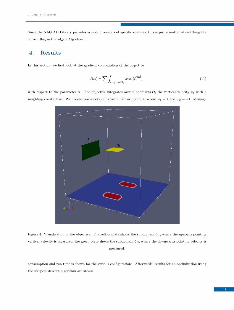
In this section, we first look at the gradient computation of the objective

J(α) =∑i

∫(x,y,z)∈Oi

wiuz(tend) . (11)

with respect to the parameter α. The objective integrates over subdomains Oi the vertical velocity uz with a

weighting constant wi. We choose two subdomains visualized in Figure 4, where w1 = 1 and w2 = −1. Memory

Figure 4: Visualization of the objective. The yellow plate shows the subdomain O1, where the upwards pointing

vertical velocity is measured; the green plate shows the subdomain O2, where the downwards pointing velocity is

measured.

consumption and run time is shown for the various configurations. Afterwards, results for an optimization using

the steepest descent algorithm are shown.

11

Adjoint Flow Solver TinyFlow using dco/c++

Configuration Run Time [s] (Forward) Run Time [s] (Reverse) Memory [MB]

passive 0.2 – (no additional)

finite differences 1152 – (no additional)

tangent 9307 – (no additional)

adjoint (fully algorithmic) 5.4 1.0 6721

adjoint (symbolic f11jc) 4.1 0.9 4963

adjoint (symbolic Newton) 2.3 0.6 2175

adjoint (fully symbolic) 1.1 0.3 84

Table 1: Run time and memory consumption for the various configurations. As can be seen, the total ratio of an

adjoint evaluation to one primal evaluation comes down to 7 for the fully symbolic case. Memory consumption

comes down to 84MB.

4.1. Gradient Computation

The following configurations can be compared:

• finite differences of TinyFlow using double

• tangent version of TinyFlow using dco/c++ tangent types

• adjoint version of TinyFlow using dco/c++ adjoint types

– algorithmic or symbolic linear solver f11jc

– explicit or implicit Euler timestepping

– if implicit Euler, algorithmic or symbolic Newton solver

As shown in Figure 5, the numerical values of the gradients computed by adjoint algorithmic differentiation and

finite differences coincide quite well for the explicit as well as for the implicit Euler.

When comparing the gradient for the different solutions with implicit and explicit Euler, the values also seem to

match quite well, see Figure 6. Tangent and adjoint versions match up to machine precision.

4.2. Topology Optimization

Availability of cheap gradient computations allows the running a steepest descent for the given objective Equa-

tion (11). The optimized α∗ is shown in Figure 7. Respective flow solutions at last timestep are shown in Figure

8.

12

J. Lotz, V. Mosenkis

(a) Full Gradient; implicit Euler. (b) Zoom; implicit Euler.

(c) Full Gradient; explicit Euler. (d) Zoom; explicit Euler.

Figure 5: Implicit Euler with ∆t = 0.1 and explicit Euler with ∆t = 0.01. Both have a resolution of 10× 10× 10

grid points. Comparison of gradient computed by finite differences and adjoint AD. The explicit case shows less

differences. This might be because of the smaller timestep (which is required for stability).

13

Adjoint Flow Solver TinyFlow using dco/c++

(a) Full Gradient. (b) Zoom.

Figure 6: Explicit vs. Implicit Euler with a resolution of 10× 10× 10 grid points: Comparison of gradient

computed with ∆t = 0.01 in the explicit case and with ∆t = 0.1 for the implicit case.

Figure 7: Visualization from two different angles of optimized α∗ for objective Equation (11). Both subdomains

are left free of any material, while the flow is actually guided by the material to the respective domains.

14

J. Lotz, V. Mosenkis

(a) Before Optimization. Streamlines through O1. (b) After Optimization. Streamlines through O1. One can see,that the flow has a larger vertical component at O1.

(c) Before Optimization. Streamlines through O2. (d) After Optimization. Streamlines through O2. The bettermatch of the vertical component through O2 is obvious.

Figure 8: Visualization of the flow solution at end time, where the objective Equation (11) is defined before and

after optimization for two different streamline sets. Material is cut of for visualization purposes only.

15

Adjoint Flow Solver TinyFlow using dco/c++

References

[1] D. Etling: Theoretische Meteorologie. Eine Einfhrung. Springer, 2008.

[2] J. Boussinesq: Theorie Analytique de la Chaleur. Gauthier-Villars, 1903.

[3] S. Raasch and M. Schroter: PALM – a Large-Eddy Simulation Model Performing on Massively Parallel

Computers. E. Schweizerbart’sche Verlagsbuchhandlung, Meteorologische Zeitschrift, Vol. 10, Nr. 5, 2001.

[4] C. Othmer and E. de Villiers: Implementation of a continuous adjoint for topology optimization of ducted

flows. 18th AIAA Computational Fluid Dynamics Conference, 2007.

[5] U. Naumann, J. Lotz, K. Leppkes, M. Towara: Algorithmic Differentiation of Numerical Methods: First-

Order Tangents and Adjoints for Solvers of Systems of Nonlinear Equations. ACM ToMS, 41(4):26:1-26:21.

[6] J. Lotz, U. Naumann, R. Hannemann-Tamas, T. Ploch, and A. Mitsos: Higher-Order Discrete Adjoint ODE

Solver in C++ for Dynamic Optimization. Procedia Computer Science, 2015 International Conference on

Computational Science.

[7] A. Griewank and A. Walther: Evaluating Derivatives, 2nd Edition. SIAM, 2008.

[8] A. Griewank and A. Walther: Algorithm 799: Revolve: An Implementation of Checkpoint for the Reverse

or Adjoint Mode of Computational Differentiation Article. ACM ToMS, 2000.

[9] S. Piascek, G. Williams: Conservation properties of convection difference schemes. J. Comput. Phys. 198,

1970.

[10] U. Naumann, J. Lotz, K. Leppkes, and M. Towara: Algorithmic Differentiation of Numerical Methods:

Tangent and Adjoint Solvers for Parameterized Systems of Nonlinear Equations, ACM ToMS, 2016.

[11] J. Lotz: Robust Adjoints of the ODE Solver d02cj. Internal Technical Report, 2018.

[12] A. Griewank and C. Faure: Piggyback Differentiation and Optimization. Large-Scale PDE-Constrained Op-

timization, Springer, 2003.

[13] B. Christianson: Reverse accumulation and attractive fixed points. Optimization Methods and Software,

Taylor & Francis, 1994.

[14] M. Towara: A Discrete Adjoint Model for OpenFOAM. Procedia Computer Science, Elsevier, 2013.

16


Recommended