Adjoint methods for option pricing, Greeks and calibration using PDEs and SDEs Mike Giles [email protected]Oxford University Mathematical Institute Oxford-Man Institute of Quantitative Finance Adjoints for finance – p. 1
Transcript
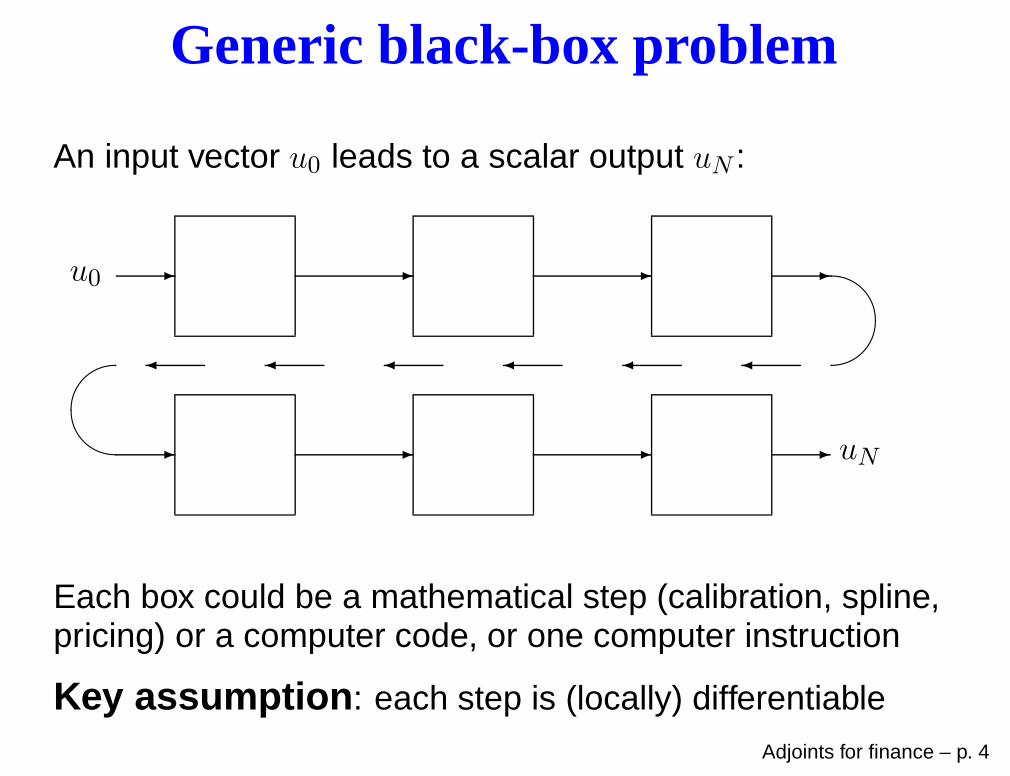
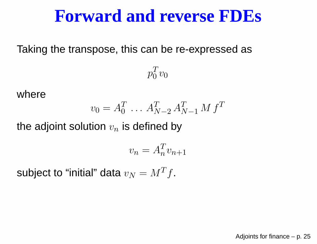
Adjoint methods for optionpricing, Greeks and calibration
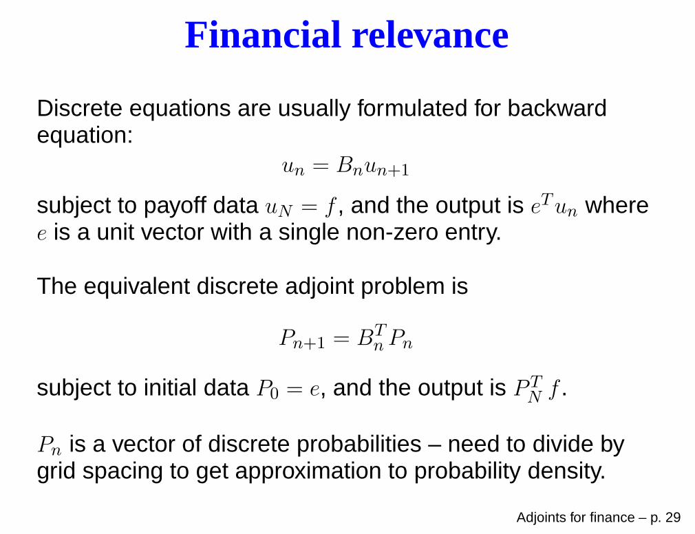
Discrete equations are usually formulated for backwardequation:
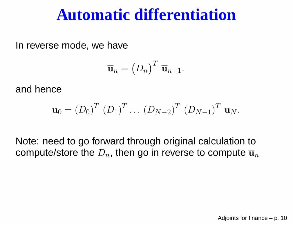
un = Bnun+1
subject to payoff data uN = f , and the output is eTun wheree is a unit vector with a single non-zero entry.
The equivalent discrete adjoint problem is
Pn+1 = BTnPn
subject to initial data P0 = e, and the output is PTN f .
Pn is a vector of discrete probabilities – need to divide bygrid spacing to get approximation to probability density.
Adjoints for finance – p. 29
Financial relevance
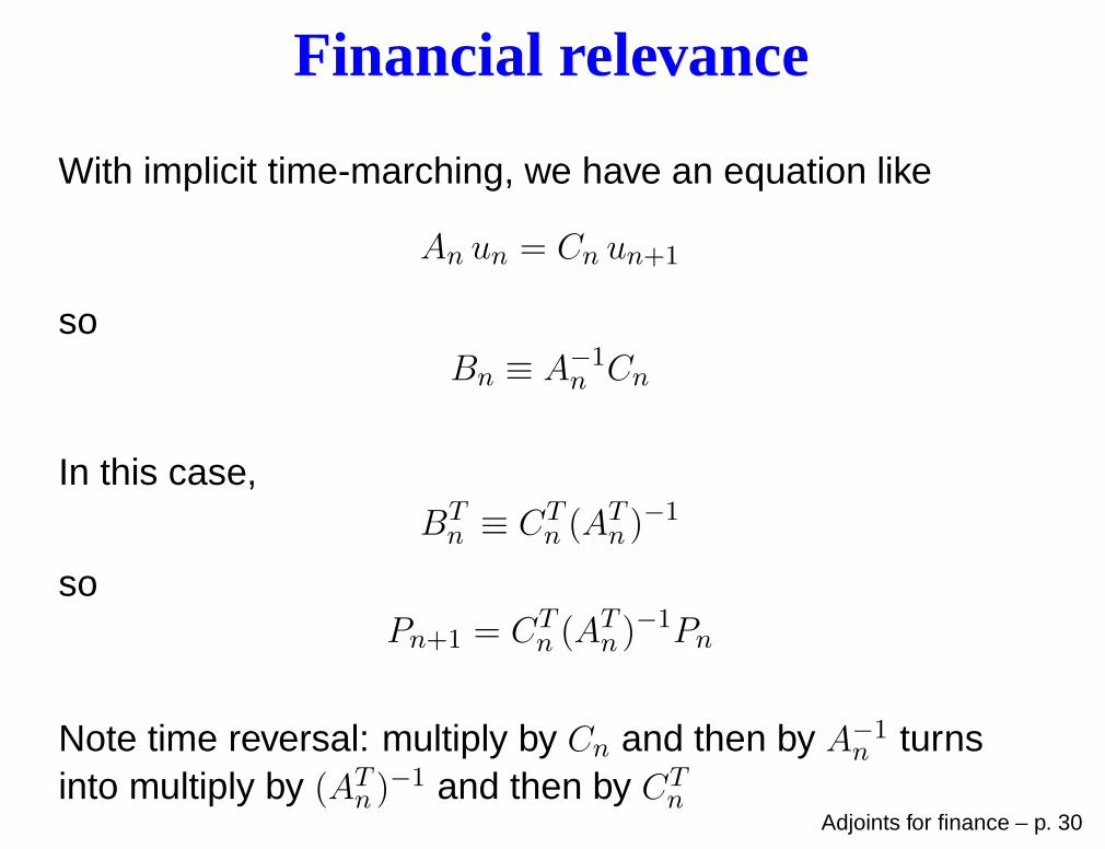
With implicit time-marching, we have an equation like
An un = Cn un+1
soBn ≡ A−1
n Cn
In this case,BTn ≡ CT
n (ATn )
−1
soPn+1 = CT
n (ATn )
−1Pn
Note time reversal: multiply by Cn and then by A−1n turns
into multiply by (ATn )
−1 and then by CTn
Adjoints for finance – p. 30
Financial relevance
Which is better – forward or reverse?
forward is best for pricing multiple European optionsa single forward calculation and then a separatevector dot product for each optionparticularly useful when calibrating a model to vanillaoptions?
backward is only possibility for American options, andalso gives Delta and Gamma approximations for free
Adjoints for finance – p. 31
FDE sensitivities
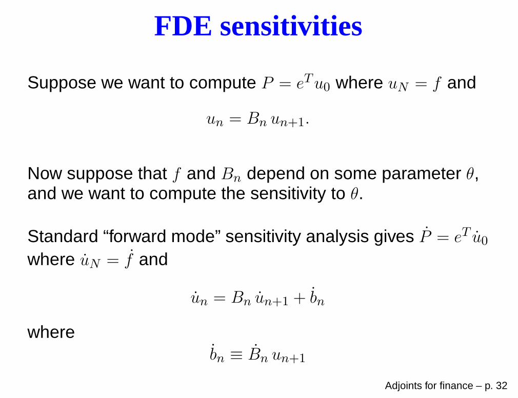
Suppose we want to compute P = eTu0 where uN = f and
un = Bn un+1.
Now suppose that f and Bn depend on some parameter θ,and we want to compute the sensitivity to θ.
Standard “forward mode” sensitivity analysis gives P = eT u0where uN = f and
un = Bn un+1 + bn
wherebn ≡ Bn un+1
Adjoints for finance – p. 32
FDE sensitivities
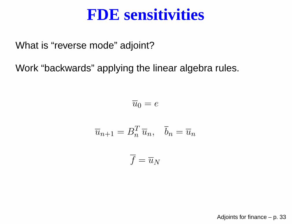
What is “reverse mode” adjoint?
Work “backwards” applying the linear algebra rules.
u0 = e
un+1 = BTn un, bn = un
f = uN
Adjoints for finance – p. 33
FDE sensitivities
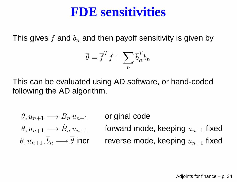
This gives f and bn and then payoff sensitivity is given by
θ = fTf +
∑
n
bTn bn
This can be evaluated using AD software, or hand-codedfollowing the AD algorithm.
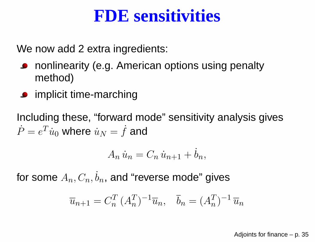
nonlinearity (e.g. American options using penaltymethod)
implicit time-marching
Including these, “forward mode” sensitivity analysis givesP = eT u0 where uN = f and
An un = Cn un+1 + bn,
for some An, Cn, bn, and “reverse mode” gives
un+1 = CTn (AT
n )−1un, bn = (AT
n )−1 un
Adjoints for finance – p. 35
FDE sensitivities
This again gives f and bn and AD ideas can then be used tocompute θ.
So far, I have talked of θ being a single input parameter, butit can be a vector of input parameters.
The key is that they all use the same f and bn, and it is justthis final AD step which depends on θ, and the cost isindependent of the number of parameters.
Adjoints for finance – p. 36
What can go wrong?
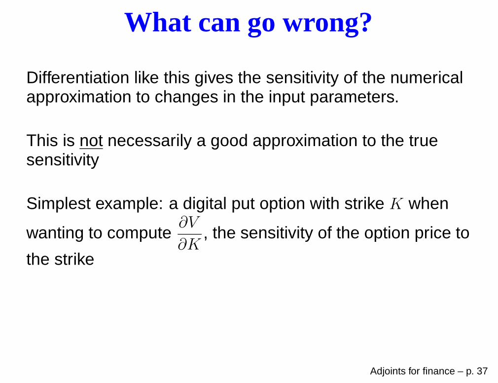
Differentiation like this gives the sensitivity of the numericalapproximation to changes in the input parameters.
This is not necessarily a good approximation to the truesensitivity
Simplest example: a digital put option with strike K when
wanting to compute∂V
∂K, the sensitivity of the option price to
the strike
Adjoints for finance – p. 37
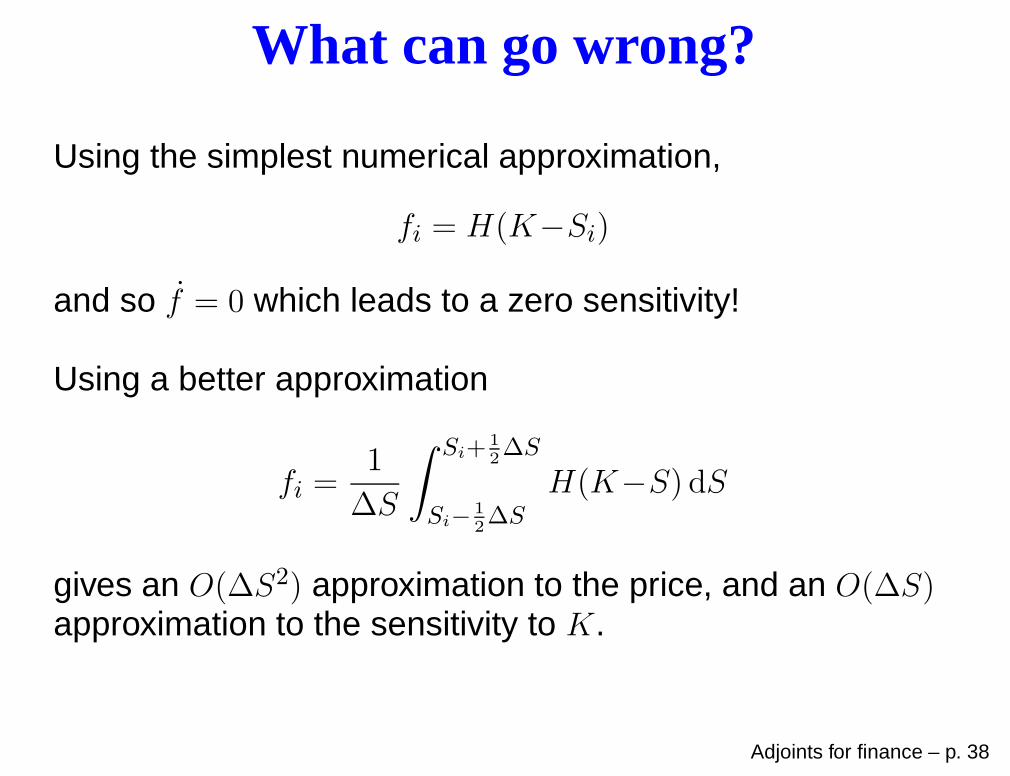
What can go wrong?
Using the simplest numerical approximation,
fi = H(K−Si)
and so f = 0 which leads to a zero sensitivity!
Using a better approximation
fi =1
∆S
∫ Si+1
2∆S
Si−1
2∆S
H(K−S) dS
gives an O(∆S2) approximation to the price, and an O(∆S)approximation to the sensitivity to K.
Adjoints for finance – p. 38
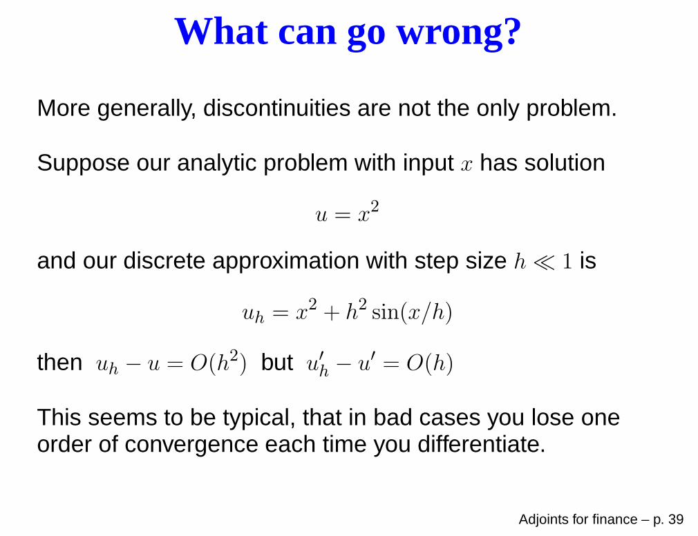
What can go wrong?
More generally, discontinuities are not the only problem.
Suppose our analytic problem with input x has solution
u = x2
and our discrete approximation with step size h ≪ 1 is
uh = x2 + h2 sin(x/h)
then uh − u = O(h2) but u′h − u′ = O(h)
This seems to be typical, that in bad cases you lose oneorder of convergence each time you differentiate.
Adjoints for finance – p. 39
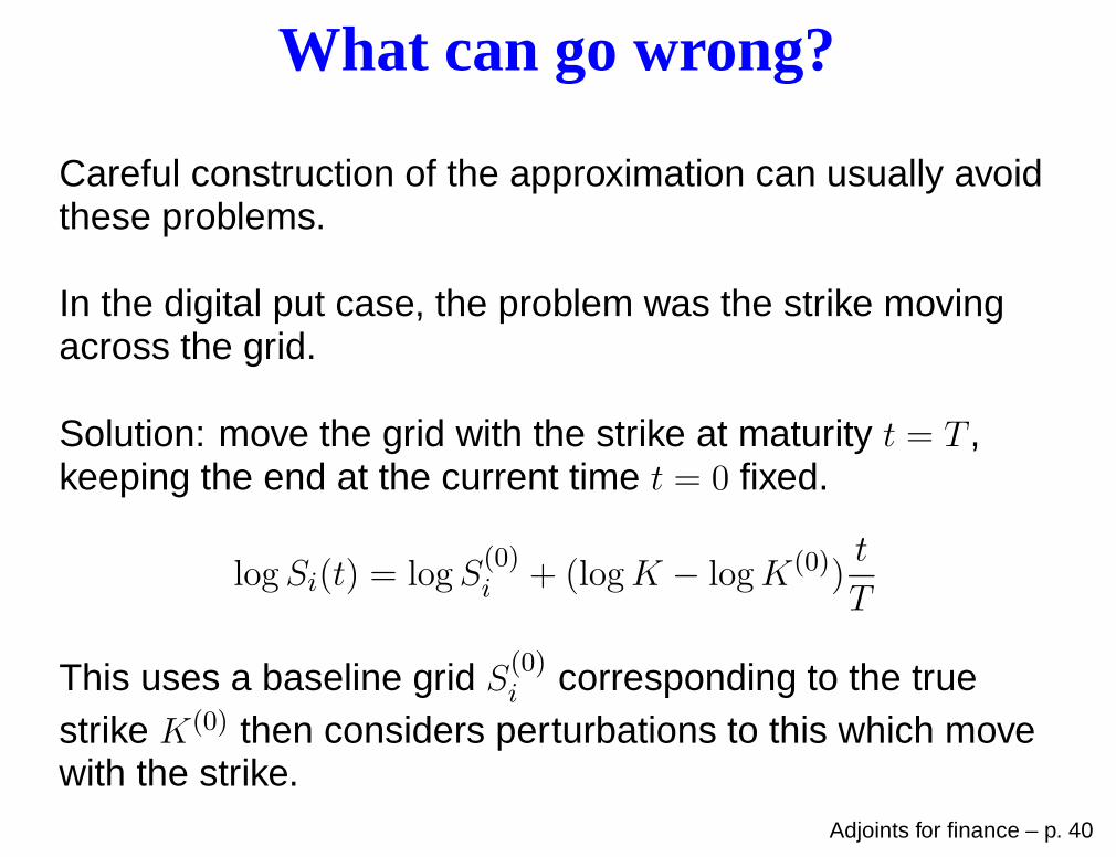
What can go wrong?
Careful construction of the approximation can usually avoidthese problems.
In the digital put case, the problem was the strike movingacross the grid.
Solution: move the grid with the strike at maturity t = T ,keeping the end at the current time t = 0 fixed.
logSi(t) = logS(0)i + (logK − logK(0))
t
T
This uses a baseline grid S(0)i corresponding to the true
strike K(0) then considers perturbations to this which movewith the strike.
Adjoints for finance – p. 40
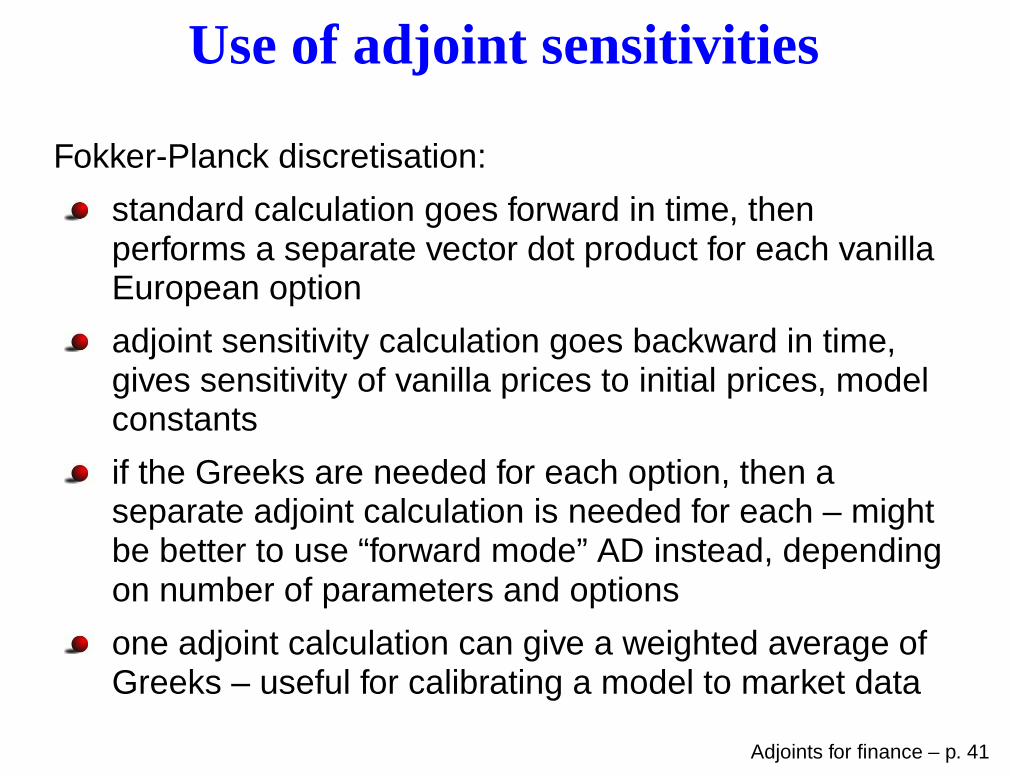
Use of adjoint sensitivities
Fokker-Planck discretisation:
standard calculation goes forward in time, thenperforms a separate vector dot product for each vanillaEuropean option
adjoint sensitivity calculation goes backward in time,gives sensitivity of vanilla prices to initial prices, modelconstants
if the Greeks are needed for each option, then aseparate adjoint calculation is needed for each – mightbe better to use “forward mode” AD instead, dependingon number of parameters and options
one adjoint calculation can give a weighted average ofGreeks – useful for calibrating a model to market data
Adjoints for finance – p. 41
Use of adjoint sensitivities
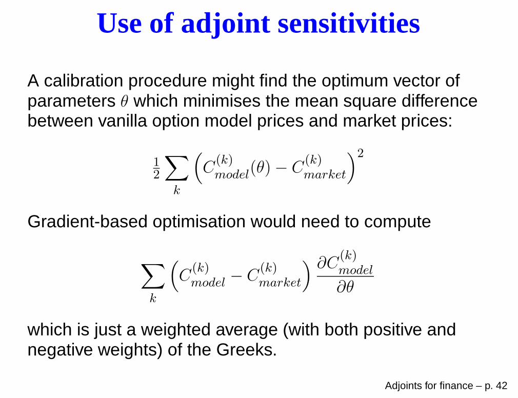
A calibration procedure might find the optimum vector ofparameters θ which minimises the mean square differencebetween vanilla option model prices and market prices:
12
∑
k
(
C(k)model(θ)− C
(k)market
)2
Gradient-based optimisation would need to compute
∑
k
(
C(k)model − C
(k)market
) ∂C(k)model
∂θ
which is just a weighted average (with both positive andnegative weights) of the Greeks.
Adjoints for finance – p. 42
Use of adjoint sensitivities
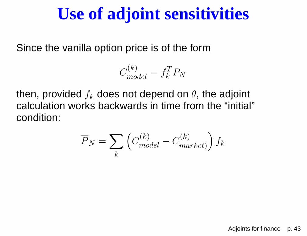
Since the vanilla option price is of the form
C(k)model = fTk PN
then, provided fk does not depend on θ, the adjointcalculation works backwards in time from the “initial”condition:
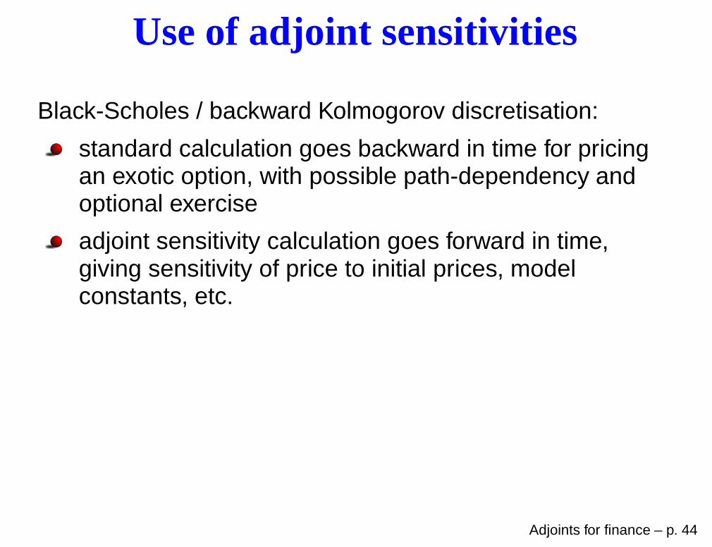
standard calculation goes backward in time for pricingan exotic option, with possible path-dependency andoptional exercise
adjoint sensitivity calculation goes forward in time,giving sensitivity of price to initial prices, modelconstants, etc.
Adjoints for finance – p. 44
Use of adjoint sensitivities
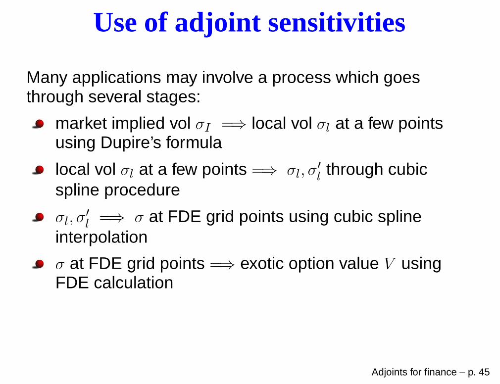
Many applications may involve a process which goesthrough several stages:
market implied vol σI =⇒ local vol σl at a few pointsusing Dupire’s formula
local vol σl at a few points =⇒ σl, σ′
l through cubicspline procedure
σl, σ′
l =⇒ σ at FDE grid points using cubic splineinterpolation
σ at FDE grid points =⇒ exotic option value V usingFDE calculation
Adjoints for finance – p. 45
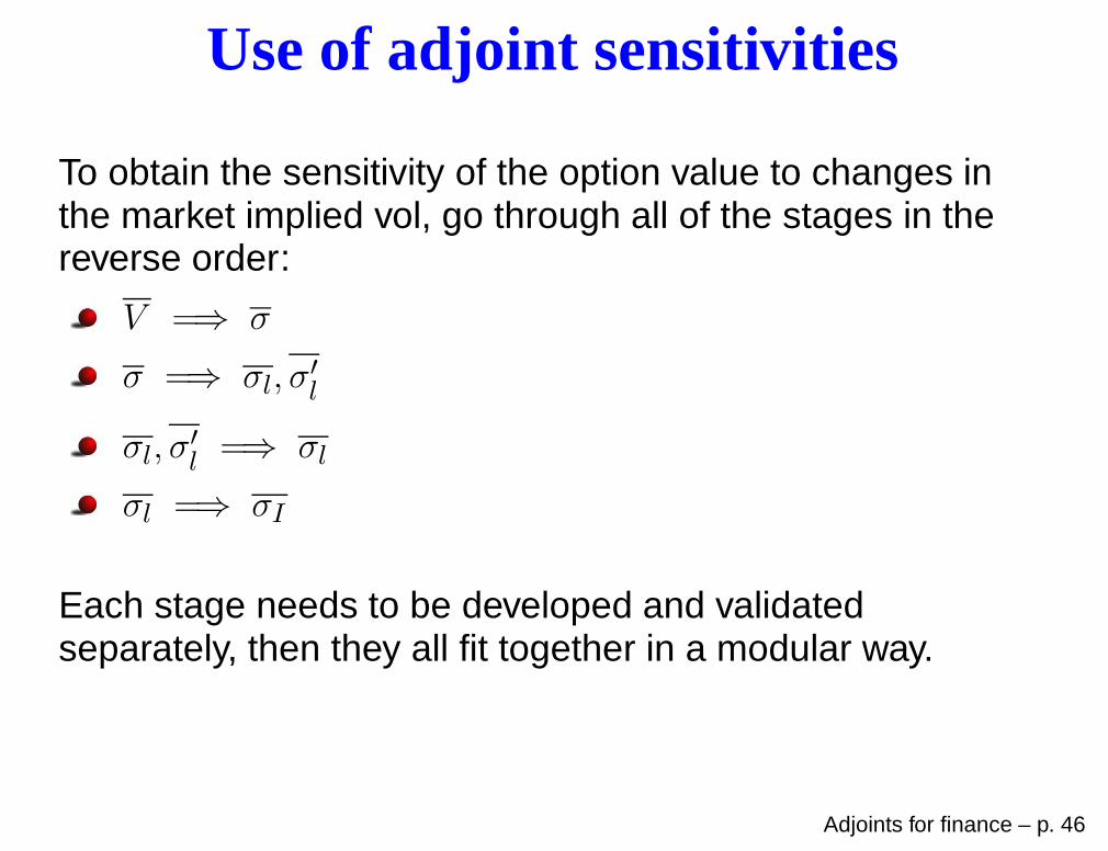
Use of adjoint sensitivities
To obtain the sensitivity of the option value to changes inthe market implied vol, go through all of the stages in thereverse order:
V =⇒ σ
σ =⇒ σl, σ′
l
σl, σ′
l =⇒ σl
σl =⇒ σI
Each stage needs to be developed and validatedseparately, then they all fit together in a modular way.
Adjoints for finance – p. 46
Use of adjoint sensitivities
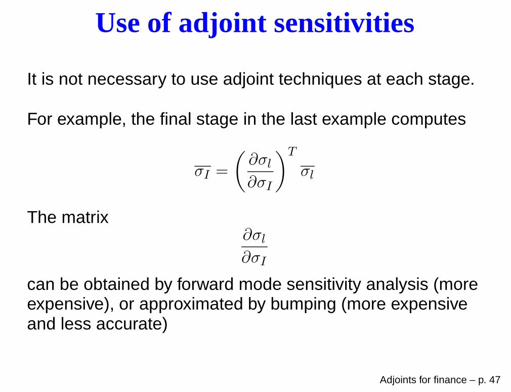
It is not necessary to use adjoint techniques at each stage.
For example, the final stage in the last example computes
σI =
(
∂σl∂σI
)T
σl
The matrix∂σl∂σI
can be obtained by forward mode sensitivity analysis (moreexpensive), or approximated by bumping (more expensiveand less accurate)
Adjoints for finance – p. 47
Monte Carlo sensitivities
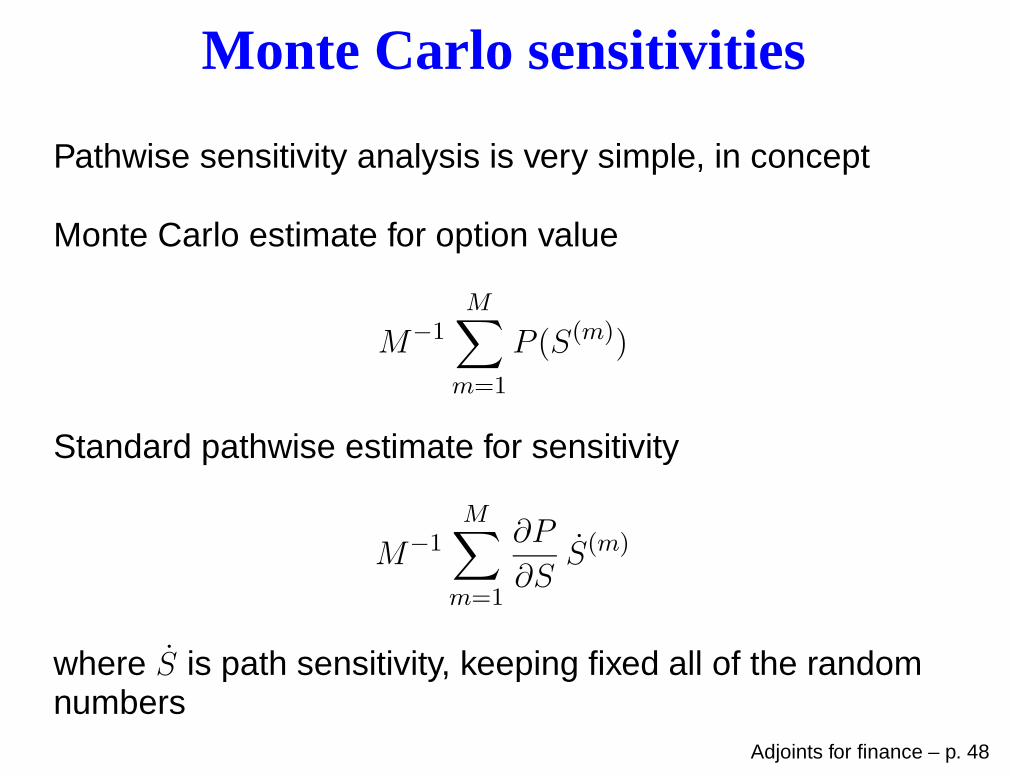
Pathwise sensitivity analysis is very simple, in concept
Monte Carlo estimate for option value
M−1M∑
m=1
P (S(m))
Standard pathwise estimate for sensitivity
M−1M∑
m=1
∂P
∂SS(m)
where S is path sensitivity, keeping fixed all of the randomnumbers
Adjoints for finance – p. 48
Monte Carlo sensitivities
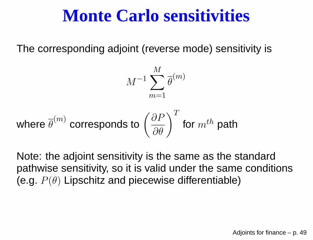
The corresponding adjoint (reverse mode) sensitivity is
M−1M∑
m=1
θ(m)
where θ(m)
corresponds to(
∂P
∂θ
)T
for mth path
Note: the adjoint sensitivity is the same as the standardpathwise sensitivity, so it is valid under the same conditions(e.g. P (θ) Lipschitz and piecewise differentiable)
Adjoints for finance – p. 49
Monte Carlo sensitivities
Largely a straightforward application of reverse mode AD,but a few new things to discuss
path-dependent payoffs (Asian and lookback options)
binning for expensive pre-processing steps(Luca Capriotti)
handling discontinuous payoffs
Adjoints for finance – p. 50
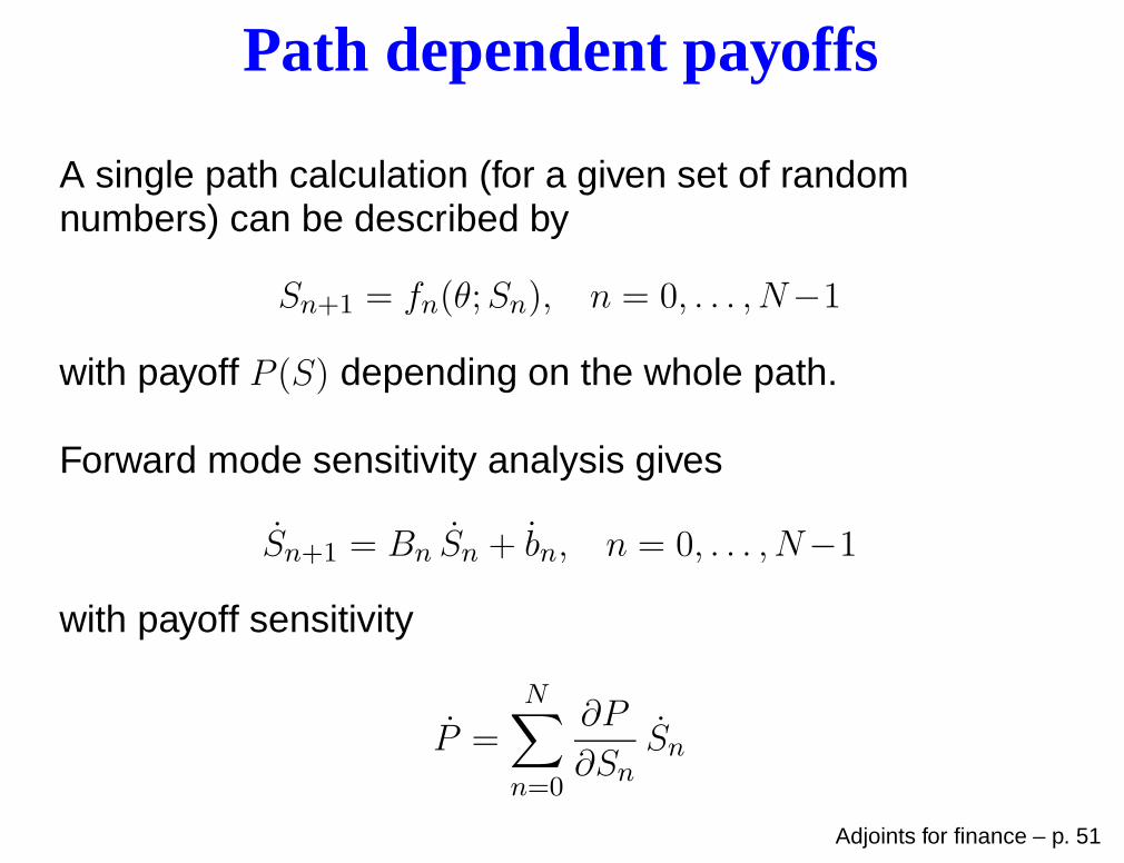
Path dependent payoffs
A single path calculation (for a given set of randomnumbers) can be described by
Sn+1 = fn(θ;Sn), n = 0, . . . , N−1
with payoff P (S) depending on the whole path.
Forward mode sensitivity analysis gives
Sn+1 = Bn Sn + bn, n = 0, . . . , N−1
with payoff sensitivity
P =
N∑
n=0
∂P
∂SnSn
Adjoints for finance – p. 51
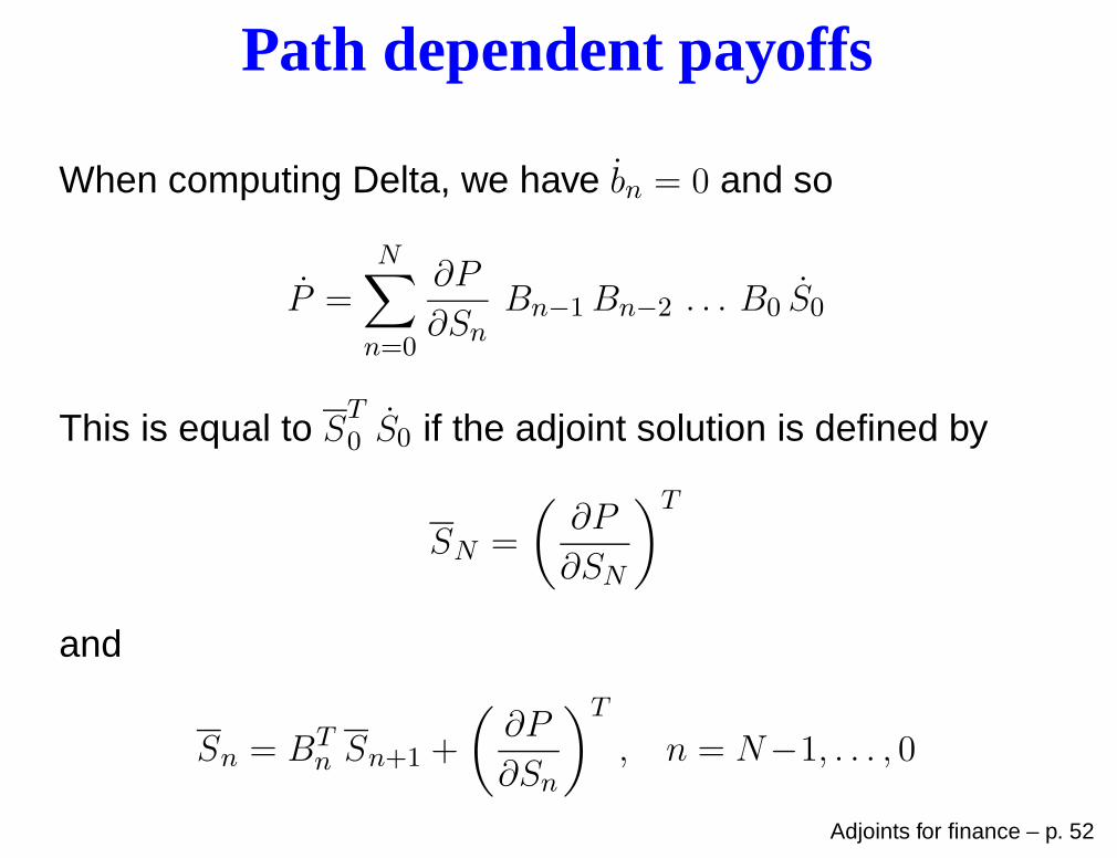
Path dependent payoffs
When computing Delta, we have bn = 0 and so
P =
N∑
n=0
∂P
∂SnBn−1Bn−2 . . . B0 S0
This is equal to ST0 S0 if the adjoint solution is defined by
SN =
(
∂P
∂SN
)T
and
Sn = BTn Sn+1 +
(
∂P
∂Sn
)T
, n = N−1, . . . , 0
Adjoints for finance – p. 52
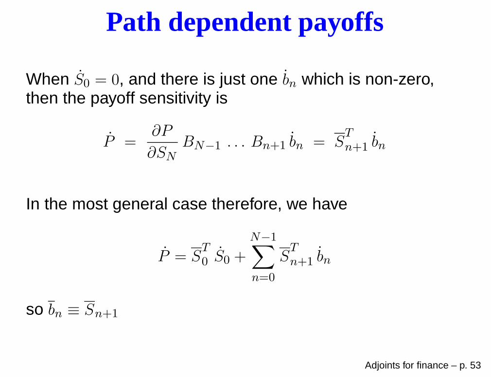
Path dependent payoffs
When S0 = 0, and there is just one bn which is non-zero,then the payoff sensitivity is
P =∂P
∂SNBN−1 . . . Bn+1 bn = S
Tn+1 bn
In the most general case therefore, we have
P = ST0 S0 +
N−1∑
n=0
STn+1 bn
so bn ≡ Sn+1
Adjoints for finance – p. 53
Path dependent payoffs
Having discussed the maths, the good news is that all ofthe details should be handled automatically by the AD tools.
If step(n,theta,S) performs the nth timestep, takingθ, Sn as input and returning Sn+1, then the adjoint routinestep b(n,theta,theta b,S,S b) takes inputsθ, θ, Sn, Sn+1 and returns an updated θ and Sn.
The only thing you have to add to Sn is(
∂P
∂Sn
)T
.
This could also be handled by AD, but maybe simpler to doit by hand – e.g. for lookback options you just need to storewhich timestep has the minimum or maximum, whereas ADwould need to store lots of other info.
Adjoints for finance – p. 54
Path dependent payoffs
An alternative point of view / approach is to make the payoffdepend only on the final state SN by augmenting the state:
∑
n
Sn for Asian options
minn
Sn,maxn
Sn for lookback options
Doing it this way, the whole adjoint code can be generatedby AD.
Adjoints for finance – p. 55
Path dependent payoffs
Some more implementation detail:
first, go forward through the path storing the state Sn ateach timestep (corresponds to “checkpointing” in ADterminology)
then, go backwards through the path, using reversemode AD for each step – this will re-do the internalcalculations for the timestep and then do its adjoint
when hand-coding for maximum performance, I alsostore the result of any very expensive operations(typically exp) to avoid having to re-do these
Note that this is different from applying AD to the entirepath, which would require a lot of storage – it’s cheaper tore-calculate the internal variables rather than fetch themfrom main memory Adjoints for finance – p. 56
Multiple European payoffs
Suppose that you have
nθ input parameters
nP different payoffs
dimension d path simulation
If nθ is smallest, use forward mode sensitivity analysis
If nP is smallest, use reverse mode sensitivity analysis
What if d is smallest?
Adjoints for finance – p. 57
Multiple European payoffs
Going back to original matrix question, what is the best wayof computing this?
· · · · ·
· · · · ·
· · · · ·
· · · · ·
· · · · ·
·
·
·
·
·
(
· · · · ·)
· · · · ·
· · · · ·
· · · · ·
· · · · ·
· · · · ·
Adjoints for finance – p. 58
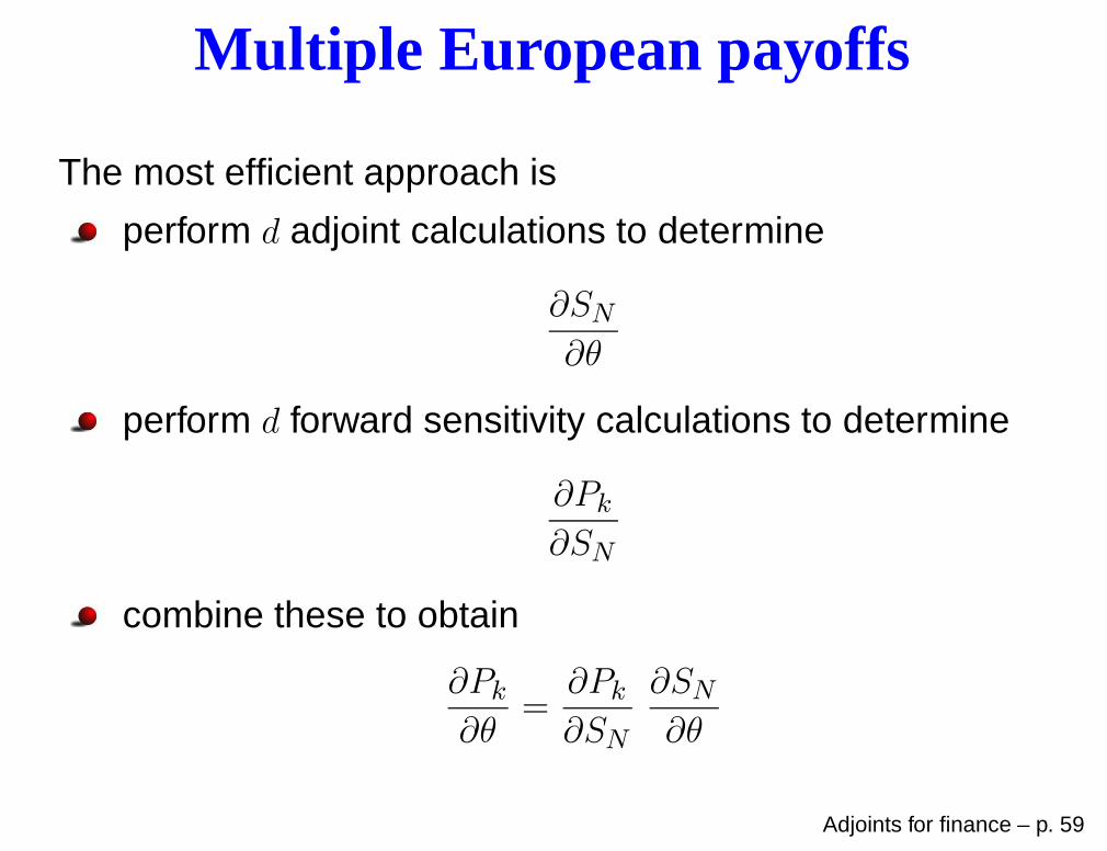
Multiple European payoffs
The most efficient approach is
perform d adjoint calculations to determine
∂SN
∂θ
perform d forward sensitivity calculations to determine
∂Pk
∂SN
combine these to obtain
∂Pk
∂θ=
∂Pk
∂SN
∂SN
∂θ
Adjoints for finance – p. 59
Binning
The need for binning is best demonstrated by the case ofcorrelation Greeks.
The standard pricing calculation has three stages
perform Cholesky factorisation
do M path calculations
compute average and confidence interval
How do we compute the adjoint sensitivity to the correlationcoefficients?
Adjoints for finance – p. 60
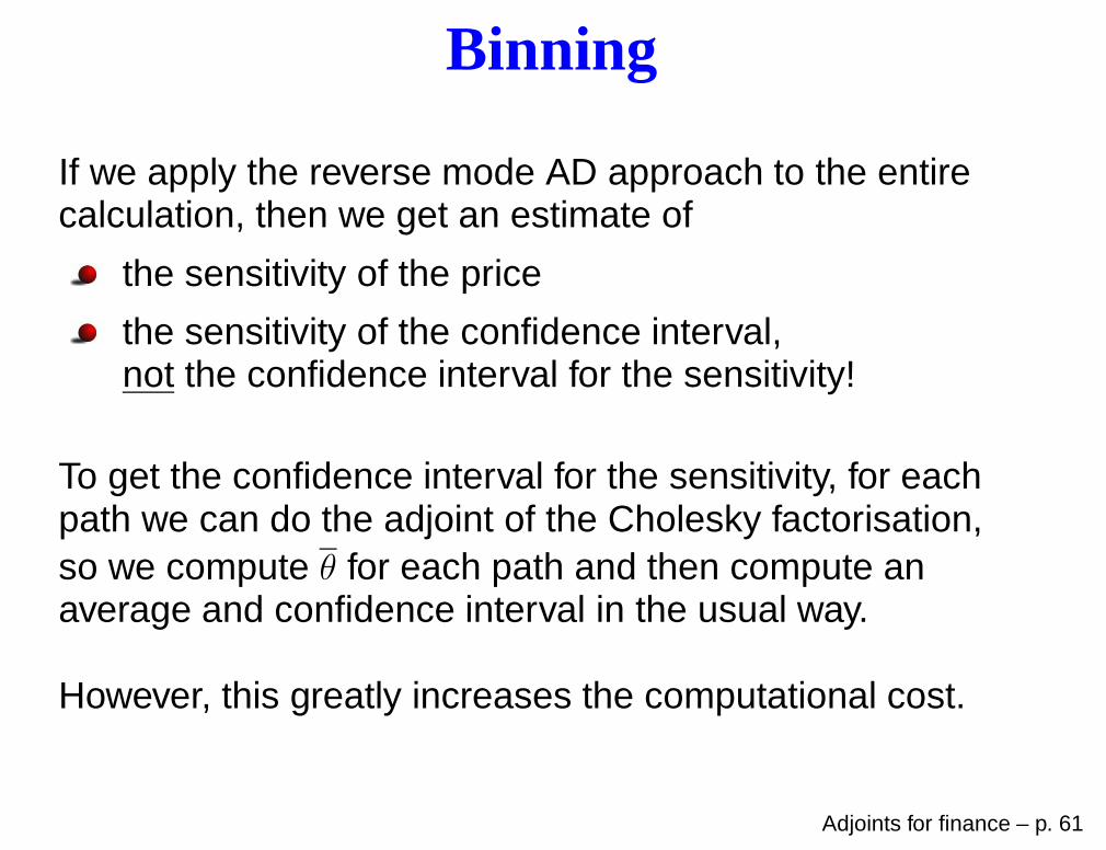
Binning
If we apply the reverse mode AD approach to the entirecalculation, then we get an estimate of
the sensitivity of the price
the sensitivity of the confidence interval,not the confidence interval for the sensitivity!
To get the confidence interval for the sensitivity, for eachpath we can do the adjoint of the Cholesky factorisation,so we compute θ for each path and then compute anaverage and confidence interval in the usual way.
However, this greatly increases the computational cost.
Adjoints for finance – p. 61
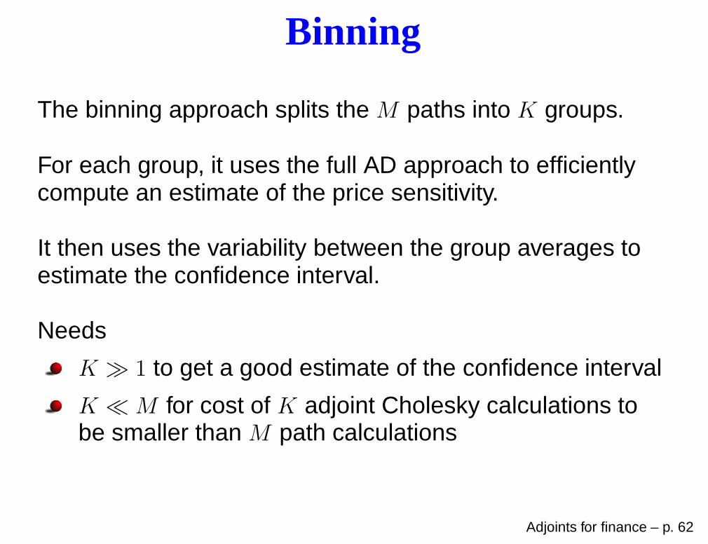
Binning
The binning approach splits the M paths into K groups.
For each group, it uses the full AD approach to efficientlycompute an estimate of the price sensitivity.
It then uses the variability between the group averages toestimate the confidence interval.
Needs
K ≫ 1 to get a good estimate of the confidence interval
K ≪ M for cost of K adjoint Cholesky calculations tobe smaller than M path calculations
Adjoints for finance – p. 62
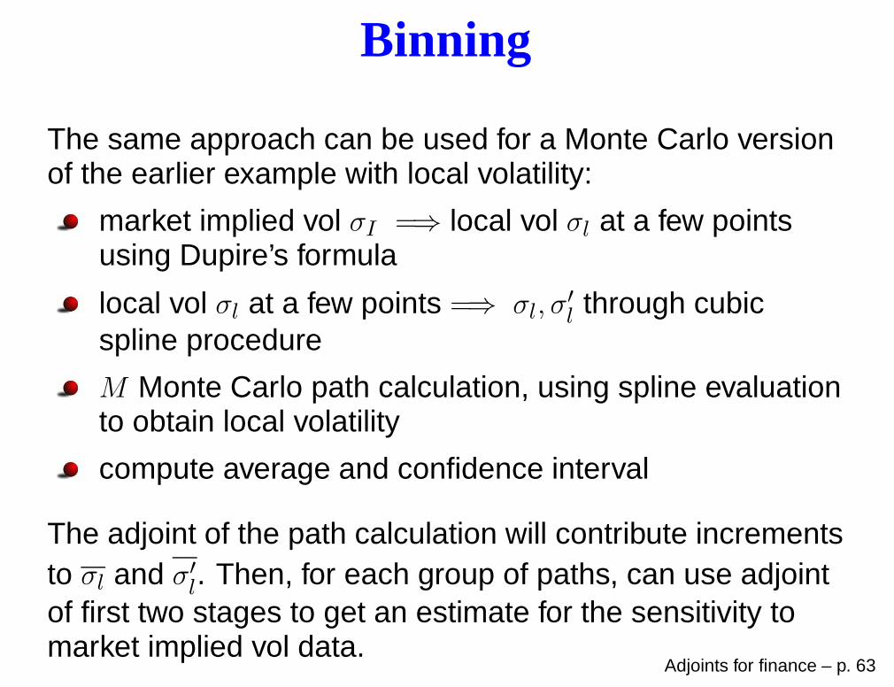
Binning
The same approach can be used for a Monte Carlo versionof the earlier example with local volatility:
market implied vol σI =⇒ local vol σl at a few pointsusing Dupire’s formula
local vol σl at a few points =⇒ σl, σ′
l through cubicspline procedure
M Monte Carlo path calculation, using spline evaluationto obtain local volatility
compute average and confidence interval
The adjoint of the path calculation will contribute incrementsto σl and σ′l. Then, for each group of paths, can use adjointof first two stages to get an estimate for the sensitivity tomarket implied vol data.
Adjoints for finance – p. 63
Non-smooth payoffs
The biggest limitation of the pathwise sensitivity method(both forward mode and reverse mode) is that it cannothandle discontinuous payoffs.
There are 3 main ways to deal with this:
explicitly smoothed payoffs
using conditional expectation to smooth the payoff
“vibrato” Monte Carlo
Of course, one can also switch to Likelihood Ratio Methodor Malliavin calculus, but then I don’t see how one gets theefficiency benefits of adjoint methods.
Adjoints for finance – p. 64
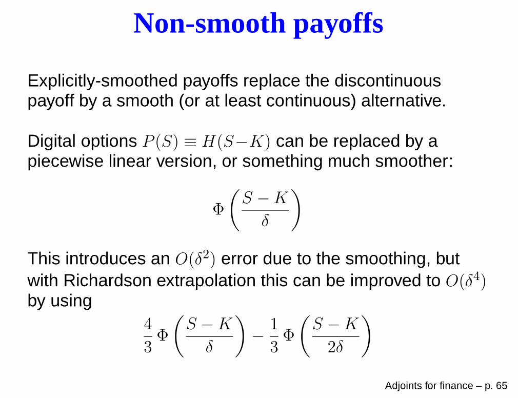
Non-smooth payoffs
Explicitly-smoothed payoffs replace the discontinuouspayoff by a smooth (or at least continuous) alternative.
Digital options P (S) ≡ H(S−K) can be replaced by apiecewise linear version, or something much smoother:
Φ
(
S −K
δ
)
This introduces an O(δ2) error due to the smoothing, butwith Richardson extrapolation this can be improved to O(δ4)by using
4
3Φ
(
S −K
δ
)
−1
3Φ
(
S −K
2δ
)
Adjoints for finance – p. 65
Non-smooth payoffs
Implicitly-smoothed payoffs use conditional expectations.
My favourite is for barrier options, where a Brownian Bridgeconditional expectation computes the probability that thepath has crossed the barrier within a timestep.(see Glasserman’s book, pp. 366-370)
This improves the weak convergence to first order, andmakes the payoff differentiable.
Adjoints for finance – p. 66
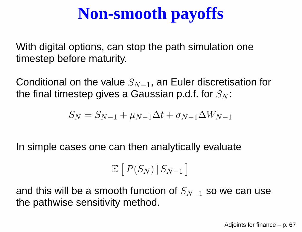
Non-smooth payoffs
With digital options, can stop the path simulation onetimestep before maturity.
Conditional on the value SN−1, an Euler discretisation forthe final timestep gives a Gaussian p.d.f. for SN :
SN = SN−1 + µN−1∆t+ σN−1∆WN−1
In simple cases one can then analytically evaluate
E[
P (SN ) |SN−1
]
and this will be a smooth function of SN−1 so we can usethe pathwise sensitivity method.
Adjoints for finance – p. 67
Non-smooth payoffs
Continuing this digital example, in more complicatedmulti-dimensional cases it is not possible to analyticallyevaluate the conditional expectation.
Instead, one can apply the Likelihood Ratio Method for thefinal step – I called this the “vibrato” method because of theuncertainty in the final value SN
Need to read my paper for full details. Its main weakness isthat the variance is O(∆t−1/2), but it is much better than theO(∆t−1) variance of the standard Likelihood Ratio Method,and you get the benefit of adjoints.
Malliavin calculus will give an O(1) variance, but no adjointefficiency gains, I think.
Adjoints for finance – p. 68
Conclusions
adjoints can be very efficient for option pricing,calibration and sensitivity analysis
same result as “standard” approach but a much lowercomputational cost
basic elements of discrete adjoint analysis are verysimple, although real applications can get quite complex
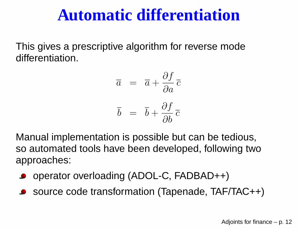
automatic differentiation ideas are very important, evenif you don’t use AD software
Adjoints for finance – p. 69
Further reading
M.B. Giles and P. Glasserman. ‘Smoking adjoints: fastMonte Carlo Greeks’, RISK, 19(1):88-92, 2006M.B. Giles and P. Glasserman. ’Smoking Adjoints: fastevaluation of Greeks in Monte Carlo calculations’.Numerical Analysis report NA-05/15, 2005.— original RISK paper, and longer version with appendix on AD
M. Leclerc, Q. Liang, I. Schneider. ’Fast Monte CarloBermudan Greeks’, RISK, 22(7):84-88, 2009.
L. Capriotti and M.B. Giles. ‘Fast correlation Greeks byadjoint algorithmic differentiation’, RISK, 23(5):77-83, 2010— correlation Greeks and binning
L. Capriotti and M.B. Giles. ‘Algorithmic differentiation:adjoint Greeks made easy’, RISK, to appear, 2012— use of AD
Adjoints for finance – p. 70
Further reading
M.B. Giles. ’Monte Carlo evaluation of sensitivities incomputational finance’. Numerical Analysis reportNA-07/12, 2007.— use of AD, and introduction of Vibrato idea
M.B. Giles. ’Vibrato Monte Carlo sensitivities’. In MonteCarlo and Quasi-Monte Carlo Methods 2008, Springer,2009.— Vibrato Monte Carlo for discontinuous payoffs
C. Kaebe, J.H. Maruhn and E.W. Sachs. ’Adjoint-basedMonte Carlo calibration of financial market models’.Finance and Stochastics, 13(3):351-379, 2009.— adjoint Monte Carlo sensitivities and calibration
Adjoints for finance – p. 71
Further reading
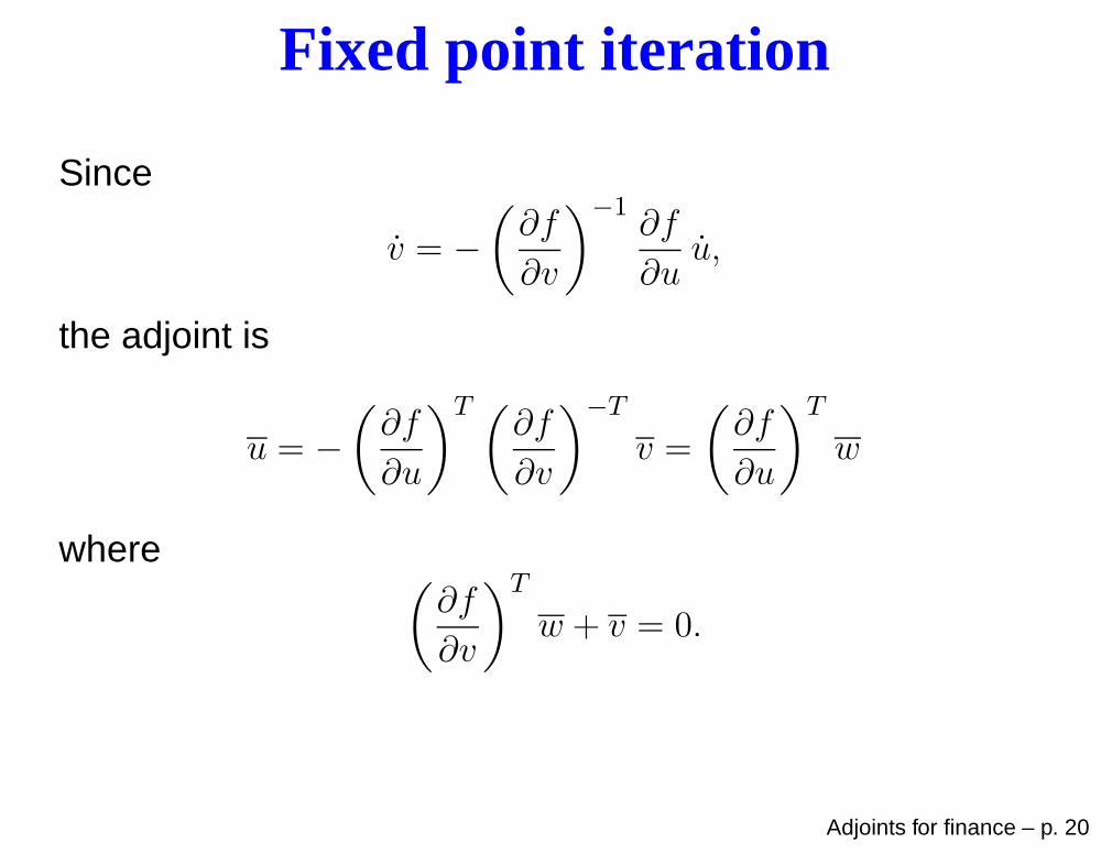
M.B. Giles ‘On the iterative solution of adjoint equations’,pp.145-152 in Automatic Differentiation: From Simulation toOptimization, G. Corliss, C. Faure, A. Griewank, L. Hascoet,U. Naumann, editors, Springer-Verlag, 2001.— adjoint treatment of time-marching and fixed point iteration
M.B. Giles. ’Collected matrix derivative results for forwardand reverse mode algorithmic differentiation’. In Advancesin Automatic Differentiation, Springer, 2008.
M.B. Giles. ’An extended collection of matrix derivativeresults for forward and reverse mode algorithmicdifferentiation’. Numerical Analysis report NA-08/01, 2008.— two papers on adjoint linear algebra, second has MATLAB code andtips on code development and validation