+ All Categories
Home > Documents > Admitting the Inadmissible: Adjoint Formulation for ... · ADMITTING THE INADMISSIBLE: ADJOINT...

Admitting the Inadmissible: Adjoint Formulation for ... · ADMITTING THE INADMISSIBLE: ADJOINT...

Date post: 29-May-2020
Category:
Upload: others
View: 30 times
Download: 0 times
Share this document with a friend
18
NASA/CR-97-206269 ICASE Report No. 97-69 , th NNIVERSARY Admitting the Inadmissible: Adjoint Formulation for Incomplete Cost Functionals in Aerodynamic Optimization Eyal Arian and Manuel D. SaIas December 1997 https://ntrs.nasa.gov/search.jsp?R=19980017376 2020-06-01T23:32:00+00:00Z
Transcript

NASA/CR-97-206269

ICASE Report No. 97-69

,th

NNIVERSARY

Admitting the Inadmissible: Adjoint Formulation

for Incomplete Cost Functionals in AerodynamicOptimization

Eyal Arian and Manuel D. SaIas

December 1997

https://ntrs.nasa.gov/search.jsp?R=19980017376 2020-06-01T23:32:00+00:00Z

The NASA STI Program Office... in Profile

Since its founding, NASA has been dedicatedto the advancement of aeronautics and spacescience. The NASA Scientific and Technical

Information (STI) Program Office plays a key

part in helping NASA maintain thisimportant role.

The NASA STI Program Office is operated byLangley Research Center, the lead center forNASA's scientific and technical information.

The NASA STI Program Office providesaccess to the NASA STI Database, the

largest collection of aeronautical and space

science STI in the world. The Program Officeis also NASA's institutional mechanism for

disseminating the results of its research and

development activities. These results arepublished by NASA in the NASA STI Report

Series, which includes the following reporttypes:

TECHNICAL PUBLICATION. Reports ofcompleted research or a major significant

phase of research that present the resultsof NASA programs and include extensivedata or theoretical analysis. Includes

compilations of significant scientific andtechnical data and information deemed

to be of continuing reference value. NASAcounter-part or peer-reviewed formal

professional papers, but having lessstringent limitations on manuscript

length and extent of graphicpresentations.

TECHNICAL MEMORANDUM.

Scientific and technical findings that arepreliminary or of specialized interest,

e.g., quick release reports, workingpapers, and bibliographies that containminimal annotation. Does not contain

extensive analysis.

CONTRACTOR REPORT. Scientific and

technical findings by NASA-sponsoredcontractors and grantees.

CONFERENCE PUBLICATIONS.

Collected papers from scientific and

technical conferences, symposia,

seminars, or other meetings sponsored orco-sponsored by NASA.

SPECIAL PUBLICATION. Scientific,technical, or historical information from

NASA programs, projects, and missions,

often concerned with subjects havingsubstantial public interest.

TECHNICAL TRANSLATION. English-language translations of foreign scientificand technical material pertinent toNASA's mission.

Specialized services that help round out theSTI Program Office's diverse offerings include

creating custom thesauri, building customizeddatabases, organizing and publishing

research results.., even providing videos.

For more information about the NASA STI

Program Office, you can:

Access the NASA STI Program Home

Page at http://www.sti.nasa.gov/STI-homepage.html

Emall your question via the Internet to

help @sti.nasa.gov

Fax your question to the NASA Access

Help Desk at (301) 621-0134

Phone the NASA Access Help Desk at(301) 621-0390

Write to:

NASA Access Help Desk

NASA Center for AeroSpace Information

800 Elkridge Landing Road

Linthicum Heights, MD 21090-2934

NASA/CR-97-206269

ICASE Report No. 97-69

bth

_,NNIVERSARY

Admitting the Inadmissible: Adjoint Formulation

for Incomplete Cost Functionals in AerodynamicOptimization

Eyal Arian and Manuel D. Salas

ICASE

Institute for Computer Applications in Science and Engineering

NASA Langley Research Center

Hampton, VA

Operated by Universities Space Research Association

National Aeronautics and

Space Administration

Langley Research Center

Hampton, Virginia 23681-2199

Ill

December 1997

Prepared for Langley Research Centerunder Contract NAS 1-97046

Available from the following:

NASA Center for AeroSpace Information (CASI)

800 Elkridge Landing Road

Linthicum Heights, MD 21090-2934

(301) 621-0390

National Technical Information Service (NTIS)

5285 Port Royal Road

Springfield, VA 22161-2171

(703) 487-4650

..............................................

ADMITTING THE INADMISSIBLE: ADJOINT FORMULATION FOR INCOMPLETE

COST FUNCTIONALS IN AERODYNAMIC OPTIMIZATION *

EYAL ARIANt AND MANUEL D. SALAS$

Abstract. We derive the adjoint equations for problems in aerodynamic optimization which are improp-

erly considered as "inadmissible". For example, a cost functional which depends on the density, rather than

on the pressure, is considered "inadmissible" for an optimization problem governed by the Euler equations.

We show that for such problems additional terms should be included in the Lagrangian functional when

deriving the adjoint equations. These terms are obtained from the restriction of the interior PDE to the

control surface. Demonstrations of the explicit derivation of the adj0int equations for "inadmissible" cost

functionals are given for the potential, Euler, and Navier-Stokes equations.

Key words, adjoint, aerodynamic optimization, Euler, Navier-Stokes, optimal shape.

Subject classification. Applied and Numerical Mathematics

1. Introduction. In recent years there has been a growing interest in solving optimization problems

governed by the Euler and the Navier-Stokes (NS) equations (for example [1]-[10]). The new interest in

this classical field is due to advances in computer performance and improvements in algorithms for the

numerical solution of the flow equations. Among the many optimization methods that are being pursued,

the Lagrange multiplier method or adjoint method is particularly attractive, because of its efficiency for

problems with many design variables. The adjoint method is based on a variation analysis of the Lagrangian

and requires that the variation vanishes at the optimum. This necessary condition yields an optimality

system of coupled PDEs consisting of the state equation, the costate or adjoint equation, the optimality

condition, and boundary conditions for the state and costate equations.

Recently, Anderson and Venkatakrishnan [8] reported some difficulties in the derivation of boundary

conditions for the costate equation for certain cost functionals. The same problem was later reported in [9]-

[10]. In [8], for example, it is concluded that for aerodynamic optimization problems which are governed by

the compressible Euler flow equations, only cost functionals that depend solely on the pressure, F -- F(p), are

admissible; and for viscous flow, using the compressible (NS) equations, only cost functionals which involve

the entire stress tensor (e.g., drag) are admissible. As stated in [8], the difficulty with the "inadmissible"

cost functionals stems from the need for a suitable balance between the different terms in the variational

form of the Lagrangian; for some cost functionals such a balance does not exist and the requirement that

the variation of the Lagrangian vanish does not result in a boundary value problem for the adjoint variables.

In [9], the authors suggest, for the compressible NS with adiabatic boundary condition on the solid wall,

to introduce a contribution into the cost functional which depends on the temperature so that appropriate

cancellation in the variation of the Lagrange functional will occur. In [10], the authors concluded that no

other choices of cost functionals, other than those suggested in [8], lead to a well-posed problem.

From the theory of functional analysis costate variables exist for all cost functionals [11]. This, however,

*This research was supported by the National Aeronautics and Space Administration under NASA Contract No. NAS1-

97046 while the authors were in residence at the Institute for Computer Applications in Science and Engineering (ICASE), M/S

403, NASA Langley Research Center, Hampton, VA, 23681-0001.

t ICASE, M/S 403, NASA Langley Research Center, Hampton, VA 23681-0001 (email: arianOicase.edu).

ICASE, M/S 403, NASA Langley Research Center, Hampton, VA 23681-0001 (email: salasOicase.edu).

is not the same as saying that all cost functionals lead to a proper boundary value problem for the costatc

equation, which is what we mean by an "admissible" cost functional.

In this paper, a general method is presented for formulating proper boundary value problcms from cost

functionals considered "inadmissible" in the literature. The method avoids redefining, or introducing new

terms in, the cost functional. Thc term "inadmissible" is obviously incorrect. We claim that for so called

"inadmissible" cost functionals additional auxiliary boundary equations are needed in the Lagrangian. These

relations are obtained from the restriction of the interior PDE and its derivatives (up to the highest order

possible) to the boundary. With these additional relations, proper cancellation of terms in the variation of

the Lagrange functional can be obtained for any well defined cost functional. However, there is value in

distinguishing those cost functionals that lead to a proper boundary value problem with out the need of

auxiliary boundary equations from those that do not. To that end, we define complete-cost functionals as

those that lead to a well posed boundary value problem of the costate equation with out need for augmenting

the Lagrangian functional with auxiliary boundary equations and we define incomplete-cost functionals as

those requiring the use of auxiliary boundary equations.

The paper is organized as follows. In §2 we begin with the potential equation and an admissible cost

functional. This example is intended to illustrate the problem that arises later with the cost functionalo•

containing _ which is also treated in this section. In §3 the adjoint equations are derived for a cost

functional containing the density, p, for shape optimization problems governed by the compressible Euler

equations. In §4 the adjoint equations are derived for a cost fimctional containing only the pressure, p,

for shape optimization problems governed by the compressible NS equations. In §5 we discuss our findings

and make some concluding remarks. Appendix A contains the definition of the Euler Jacobian matrices.

Appendix B contains identities of polar coordinates which are used extensively in §§3-4. Appendix C contains

a demonstration of the adjoint derivation on a more complex cost functional, than the one presented in §4,

for shape optimization problems governed by the compressible NS equations.

2. The Potential Equation. Let _t bca two dimensional domain confined in the area between two

circles with radii R1 < R2. We denote by F the circle with radius R1 and by 01"t - F the circle with radius

R2. Let f*(_) be a given L2(F) function defined on the boundary F, and let the function a(_), defined on

F, be the design variable.

2.1. An "Admissible" Cost Functional. Consider first the derivation of the adjoint equation on a

Dirichlet cost functional using the standard procedure. The minimization problem is defined as follows:

minFl(¢)-- fr (¢- f*)2da(2.1)

subject to

(2.2)A¢----0 inft

oaOn = -'_ on F

¢=¢o on 0_- F

where n and t, respectively, denote the outer normal and tangential directions on the boundary F. The

definition of the state equation (2.2) assumes the following smoothness properties:

a E H I(F)

(2.3) ¢ • HI (_),

whereH k denotes the Sobolev space of order k (see [12]). The necessary conditions for a minimum are

derived with the adjoint method. We introduce the Lagrange multipliers A defined on the domain f_,

defined on part of the boundary F, and _ defined on the rest of the boundary al2 - F. In terms of the

Lagrange multipliers, a Lagrangian is defined by:

The variation of the Lagrangian is given by:

The term containing ¢ on 0f_ - F was omitted since ¢ is fixed on that part of the boundary (see Eq.(2.2))

and therefore its variation vanishes.

The necessary conditions for a minimum are obtained by requiring that the integrands in (2.5b) vanish.~

Matching the terms that multiply ¢, and those that multiply _-_, results in the following equations:

¢(_): AA=0 inoA__(r): _ - -2(¢-/*) on r

(r): ¢= _ onr(0_ - r) : _ = 0 on 0_ - r

_(r): _ = 0 onr.

Therefore, the costate (adjoint) boundary value problem is defined by

AA = 0 in

(2.6) oh _- -2(¢- f*) on rA=0 on 0_ - F,

with the Frdchet derivative of the cost functional with respect to a given by

(2.7) dF1 Ohda - cOt on F.

2.2. An "Inadmissible" Cost Functional. Suppose that we want to minimize a cost functional that

depends on the second normal derivative on the boundary. Then the minimization problem is defined as

follows:

(2.8) mjnF_(_)= - f-j _

subject to Eq.(2.2). However, the definition of the cost functional (2.8) assumes that the second normal

derivative of ¢ on the boundary exists and is in L2(F). This is not consistent with the smoothness requirement

of ¢, (2.3), unless we additionally assume that a is smoother than required by the state PDE, i.e.,

(2.9) a e H=(r)¢ E H_ (f_).

If wederivethenecessaryconditionsfor aminimumaswedid for theDirichletcostfunctional(2.1),thenthevariationoftheLagrangianisgivenby:

(Aspreviouslydiscussed,thetermthat contains¢ onthe "far-field",0f_ - F, was omitted.)

In the previous example, we saw how the first and third terms in the variation of the Lagrangian (2.5a)

combined to give a boundary condition for 0_ along F. In this example, the first term in (2.10), the term_nn02-

with -_, can not be combined with any of the other terms on the boundary F and, hence, we can not obtain

a boundary condition on F for the costate equation. A cost functional exhibiting this behavior was termed

"inadmissible" in the literature [8]. However, since the state equation (2.2) is linear, ¢ depends on c_ linearly,

the cost functional F2 is a quadratic in _. A quadratic cost functional has a unique minimizer, thus the cost

functional F2 is in-fact admissible.

In the next subsection, we show how to overcome this problem using an auxiliary boundary equation.

2.3. Auxiliary Boundary Equation (ABE). For convenience, let us introduce polar coordinates

(r, 0). In polar coordinates, thc restriction of the interior PDE (2.2) to the boundary F results in the

following ABE (assuming the consistency requirements of (2.9))

(2.11) i% Or + + _-_t_-_ = 0 on F.

Here we assume that _ = -fi is perpendicular to the boundary, pointing into the domain, and R1 is the

radius of curvature. By Eq.(2.11) we get (dt = R:dO)

. . 02-

(2.12) -_: (-_-7_-_-t) onr,

which can be used to replace _ in the variation of the Lagrangian. Integration by parts, along the boundary,

of the term containing tangential derivatives results in a variational form of the Lagrangian which contains

only the naturally occurring boundary terms (¢ and _).

Another way to use Eq.(2.11), which leads to the same result, is by adding it to the Lagrangian with a_ - 82-

new Lagrange multiplier 7. Then/_ is augmented with the term frr_ ( - _ _r - _ - _-t ) da which results

in the following adjoint equations on the boundary:

(2.13) $(r) : _ _ _ :-°__ 0-_(r) : :_-_+¢=0.

Therefore, the adjoint equations can be written in the following "strong" form:

(2.14)

AX=0 in f_

or = 2 - on F

)_=0 on 0f_ - F.

The Prdchet derivative of the cost functional F2 with respect to _ is then given by

_F2 0¢ oh 2 { 03¢ of*(2.:5) -_ = Yi = gi - _ _o-_t -_ ) o. r.

In the same manner other cost functionals can be treated by taking (if necessary and consistent with

the smoothness assumption of the cost functional definition) higher derivatives of, A¢ = 0, restricting the

resulting equations to the boundary and adding them to the Lagrangian with additional Lagrange multipliers.

We add a remark on the required smoothness of the Lagrange multipliers. If we insist in solving the

adjoint equation in its "strong" form (2.14), then the smoothness requirement of the state solution should

be even stronger than (2.9) (also if(s) should be smoother than L2(F)). This requirement can be relaxed

if the adjoint equations are solved in a weak formulation, for example, by finite elements [11]. For future

reference we give here the following definition.

DEFINITION 2.1. We define a complete-cost functional as one that leads to a boundary value problem

of the costate equation with out the need for augmenting the Lagrangian functional with auxiliary boundary

equations. Otherwise, the cost functional will be termed as incomplete.

In the next sections we treat similarly higher level models of fluid dynamics PDEs. In these cases, the

functional analysis of the smoothness properties of the state equations are not as obvious as in the above

example.

3. The Euler Equations. For simplicity the derivation is done in two dimensions. Let U denote the

vector of state variables:

(3.1) U = (p, pu, pv, pE) T,

where we use the following notation: p denotes the density, ff = (u, v) denotes the velocity vector, and E

denotes the total specific energy.

The Euler equations are given by (conservative form)

div(pff) = 0

(3.2) div(pff @ ff + pI) = 0

div(pffH) = 0

where if- ff = 0 on the solid wall F, and with additional appropriate boundary conditions on the far-field.

(The above system, in the interior, can be written in an equivalent form in terms of the Jacobian matrices,

V(._[7) = 0, where ._ = (A, B) denote the Jacobian matrices given in appendix A.)

The following are state relations for the pressure, p, and the total enthalpy, H:

vlul(3.3) P=(7-1)pE-_ "2H = __7__v+ lal2

•_--lp 2 "

3.1. Natural Boundary Terms. Integrating by parts the Euler equations results in a term containing

the pressure on the boundary:

(3.4) f_ V(.4[?)df_ =/aep(0 , nl, n2, 0) Tdo',

(in polar coordinates nl = -1 and n2 = 0), therefore any minimization problem that contains terms other

than the pressure will result in non-canceling terms in the variational Lagrangian.

3.2. Example of an Incomplete Cost Functional. The following cost functional is incomplete (the

design variable is the shape of the solid wall F):

(3.5) F(p) = [(p - p*)2da.Jr

The Lagrangian is given by

(3.6) £: = fr(P - P*) 2da + f_ ATv('4U)dfl + fr _(ff" _)da+ far-field terms,

where ,_ is the vector of costate variables,

(3.7) /V,= ()`1,)`2, ),3, )`4) T

and we denote by _ the adjoint "velocity" vector, i.e.,

(3.s) =

The variation of the Lagrangian is given by

(3.9) _ = fr 2/5(p - p*)da + fn _(ATp,= + BT._y)d_ + frfA2dcr + fr &g(U, 5.)da+ far-field terms,

which results in non-cancellation of terms in _, since the cost functional is not given in terms of the natural

boundary term p 1.

However, in general we can write

(3.10) p = p(p, s)

where s is the entropy and, in particular, on the surface F we can write

(3.11) p = p(p)

in the absence of shock waves 2, since the entropy is constant along the streamline wetting the surface.

Hence, we know that we can overcome this problem. In the next section we derive the adjoint equations, for

the incomplete cost functional (3.5), with a general procedure, along the lines of §2.3.

3.3. Auxiliary Boundary Equatlons. As in the potential problem we derive auxiliary boundary

equations (ABEs) by restricting thc interior PDEs to the boundary. For simplicity, we examine the result-

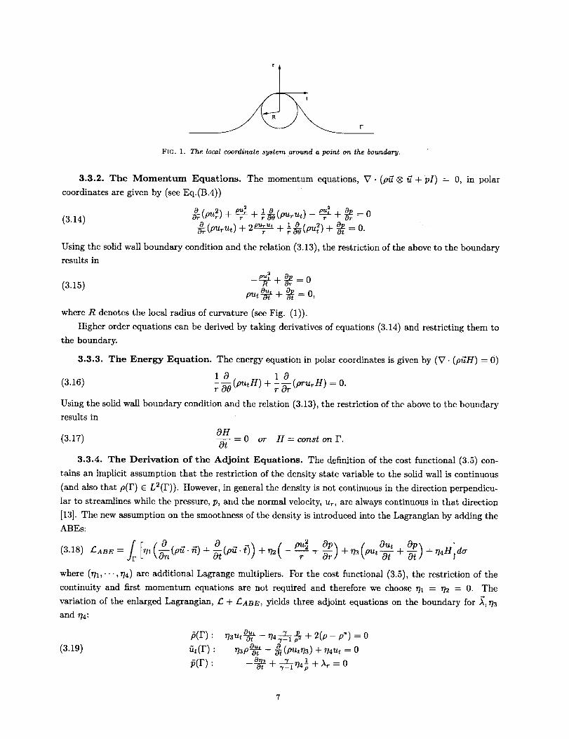
ing equation locally around a point on the b0uncla'ryand_-use polar coordinates. Fig.(1) depicts the ]ocai

coordinate system. Throughout the paper we use the unit tangential vector t'on the boundary instead of 8.

Note that on the boundary, F,

0 1 0

(3.12) O-t = R ¢30"

Also, in polar coordinates the components of the velocity vector _7will be denoted by _7 = (ur, u,) where

u_ = ft. _" and ut = _7.8; similarly, the components of the adjoint "velocity" vector _ will be denoted by

= ()`_,)`t) where )`r = _" r' and )`, = _- _.

3.3.1. The Continuity Equation. In polar coordinates, on the boundary, the continuity equation is

given by (V(frE) = 0) .......

0 0

(3.13) _rr (purl + -_(pu,) = O.

Also higher order derivatives of the continuity equation can be taken and restricted to the boundary and

are considered auxiliary boundary equations, as long as the solution in the interior is smooth enough so that

these derivatives exist.

1In fact, for shape optimization problems, as we discuss here, the variation of the Lagrangian includes more terms on the

boundary F that depend on _. _. However, these terms contribute only to the gradient term fr &g(U' .E,)da and therefore donot play a role in the derivation of the adjoint boundary value problem. For simplicity we do not discuss these terms in this

paper.21n the presence of shocks, it is still valid to write p --- p(p) in a piecewise sense between shocks using the Rankine_Hugoniot

conditions to connect the piecewise regions along the streamline wetting the surface.

FIG. 1. The local coordinate system around a point on the boundary.

3.3.2. The Momentum Equations. The momentum equations, V • (pff ® ff + pI) = 0, in polar

coordinates are given by (see Eq.(B.4))

o 2 _ 10, u _ .__ _=0(3.14) _7(PUr) + r + ;_-_(pUr _/- r + Or

O (purut ) 2__r__ 1 a, u 2, op = O.+ _ + _-_(P t) + a_

Using the solid wall boundary condition and the relation (3.13), the restriction of the above to the boundary

results in

_ed+ =0(3.15) R or

^u o_ o_ =0,P t at 3-- o_

where R denotes the local radius of curvature (see Fig. (1)).

Higher order equations can be derived by taking derivatives of equations (3.14) and restricting them to

the boundary.

3.3.3. The Energy Equation. The energy equation in polar coordinates is given by iV" (p_TH) = 0)

1 a 1 c9(3.16)

- 0-0 (putS) + - X (pru_U) = O.r r

Using the solid wall boundary condition and the relation (3.13), the restriction of the above to the boundary

results in

(3.17) --0H=0 or H=constonF.Ot

3.3.4. The Derivation of the Adjoint Equations. The definition of the cost functional (3.5) con-

tains an implicit assumption that the restriction of the density state variable to the solid wall is continuous

(and also that p(F) E L2(F)). However, in general the density is not continuous in the direction perpendicu-

lar to streamlines while the pressure, p, and the normal velocity, ur, are always continuous in that direction

[13]. The new assumption on the smoothness of the density is introduced into the Lagrangian by adding the

ABEs:

_r 0 pu_ Op _?3(pu OUt Op _?4H]da

where (_1,''', I]4) are additional Lagrange multipliers. For the cost functional (3.5), the restriction of the

continuity and first momentum equations are not required and therefore we choose _h = v]2 -- 0. The

variation of the enlarged Lagrangian, l: +/:ABe, yields three adjoint equations on the boundary for _, r]3

and r/a:

(3.19)

#(r):_t(r):

+ 2(p-p*)= 0_^_-_ - o_(putVa) + _4ut = 03P Ot

where wc have used the relation 3

"7- 1 - p'2P + utfit = 0.

The above system can be solved by solving the first two PDEs in (3.19) for 73 and 774 and substituting the

result in the third equation which is the transpiration boundary condition for A.

4. The Navier-Stokes Equations. The compressible NS equations are given by

div(pg) = 0

(4.1) div(p_7 ® if) = div(a)

div(ea) + div(q")= di ( g)

where the stress tensor, a, is given by

a = -pI + #2div(g)I + #def(_,

and I denotes the unit tensor, def = grad + grad T, and # and #2 are the first and second viscosities,

respectively (#2 + 2p _- 0). The vector g denotes the heat conduction vector, g = -kgrad(T), where T3

denotes the temperature, and k denotes the coefficient of conductivity and will be set equal to a constant.

The total energy satisfies e = p_21_ + p_-_.

The solid wall boundary conditions are given by :

g=0

(4.2) aT + b-_n = c

where a, b and c are parameters (in this paper we set a = c ----0 and b -- 1, resulting in the adiabatic

wall boundary condition).

4.1. Natural Boundary Terms. For simplicity we will denote the system of NS equations by V.F = 0.

where F consists of the flux vectors. Integration by parts of the compressible NS equations results in the

following boundary terms:

(4.3) _ (V " ff)dl_ = _o (O, (aff)l , (aff)2, 0)T da.

Therefore, the natural boundary terms for the compressible NS equations are the total fluid force components,

(aff)j. (In other words, the only complete cost functionals are those which measure lift or drag.)

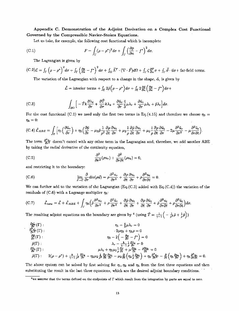
4.2. Example of an Incomplete Cost Functional. Let us take, for example, the following cost

functional which is incomplete (here, as in the previous section, the design variable is the shape F) since its

variation is not given in terms of the force components in (4.3):

= f(p - p') do.(4.4) F(p)

The cost functional (4.4) was treated previously in [14] by neglecting a term in the Lagrangian and in [8] by

modifying the cost functional. A demonstration of the adjoint derivation on a more complex cost functional

is given in appendix C.

3we assume that the term defined on the endpoints of F which re_u|ts from the integration by parts, fr _3 ao-_tda, is equal to

zero, i.e., _3p(0F +) - _3p(0F-) = 0.

The Lagrangian is given by

• rOTdvr(4.5) F. = fr(P - P*) 2da + fn _T (V" fi)df_ + fr _-_ _- fr ¢. ffda+ far-field terms.

The variation of the Lagrangian is given by

= interior terms + fr 2_(p - p*)da+

(4.6) Ion [- ¢k_2 + _ ^4 _ _.g-__,_r + or " , + + fr

o_ does not contribute to the adjoint equations (assuming adiabatic boundary conditions) andThe term _-

therefore will be omitted (by the same reasoning the term containing the variation of ff on F and the variation

of the far-field terms vanish)• Also note that the variation in T can be transformed to variations in p and

p using the equation of state, T = _o' The cost functional (4.4) is considered incomplete since the term

determines the adjoint boundary condition Ar = 0. As a result we do not obtain a boundary valueOr

problem representation of the adjoint equations.

4.3. Auxiliary Boundary Equations.

4.3.1. The Continuity Equation. Since the boundary condition on F implies that °(put) = 0, we

get from the continuity equation that (see Eq.(3.13))

(4.7) Our0---_ =0.

4.3.2. The Momentum Equations. Let us write the momentum equations in the form

div(pff ® if) = div(cr) = div(-pI) + div(_-).

The term div(pff ® ff + pI) is given in polar coordinates in Eq.(3.14). Taking the limit to the boundary we

get that

lim div(pff @ if) = 0._--*F

The term r in polar coordinates is given by

(#2div(ff)+2#_ [o___ _-__' )

- r *(4.8) r = #2div(ff)I + #def(ff) = [ou. _ - ou___'_

#_:--_- - r -t- or ) #2div(ff) + 2#(-_t + -_:)

Evaluating div(r) on the boundary and using the identities

lime-_r div( g) = 0

(4.9) lim_r ° div(ff) = -_ ot Or

results in the following auxiliary momentum boundary equations (see Eq.(B.4))

or+ .. - ". o'.._ . o_ o o,= o(4.1o) o,..- #-a--_/- _# Or = 0.

4.3.3. The Energy Equation. The energy equation is given by

div(eff) + div(q-) = div(aff).

Using the relation

and taking its divergence in polar coordinates we get

(4.11) lim div(eff) = O.x_---_F

The term div(q-) = -kAT satisfies (assuming an adiabatic boundary condition)

, 3(4.12) e--rlimdiv(q-) = -k(-ff_r2 + Ot2/.

The term aft and its tangential derivatives on the boundary are zero, therefore only its radial derivative

is considered:

(4.13) lim div(aff) = #( Out _ 2_r _, Or / "

Eqs. (4.11)-(4.13) imply the following auxiliary energy boundary equation

.102T 02T _ / Out _2(4.14) --k(_-_r2 + Ot 2 ] - #_,Or ) = O.

4.3.4. The Derlvatlon of the Adjoint Equations. As in the Euler case, we add the ABEs to the

Lagrangian:

_r 1 019 OUt 02_tr 021it "_k Or / p Ot Or 2_-g_-r2- _-g-_)

02u_ 1 Out _ I z O2T 02T _ Out 2(4.15) -t-r/3 (_--_ -it Or s -R#--_r ) + _a [ - k _-_r2 + -_ ] - # (-_r ) )Ida.

However, for the cost functional (4.4) we need only the first term in Eq.(4.15) and therefore we choose

rt2 = _ = rl4 = 0:

[` + [-ABE = interior terms + fr 215(p -- p*)da+

a__:/ _tr #At + iSAr] dg fr &gl(_,/_ '(4.16) fort [- TkO_ + or _,rh + _#Ar) + + rh)da.

The variation of the enlarged Lagrangian, L: + 12ABE, yields the following equations on the boundary (using

fP/ 4Or k-- I : 771 -J- g _t'_r = 0

/5(F): 2(p-p*)+A_ k 1__ =0

(4.17) _¢(r) : .x_ = 0k 1 o____

_(r) : _-_ _ o_ = 0.

The resulting adjoint equations on the solid wall are given by (See Eq.(4.2))

x_ = -2(p - p')

(4.18) A_ = 0

db-¢ _- 0.dn

l0

Note that the first equation in (4.17) determines the auxiliary Lagrange multiplier _1:

4 A 8(4.19) _71-----5# r =- 5#(P - P*).

That Lagrange multiplier is affecting the gradient, gl = gl(U,A, _71), since the variation of the continuity

auxiliary boundary equation (4.7) with respect to a change in the shape, F, results in variational boundary

terms that multiply only the term &.

5. Discussion and Concluding Remarks. We present a method for the derivation of the costate

equations for problems in which the cost functional does not lead to a proper boundary value problem for

the costate equation, when derived in the standard way. We define such cost functionals as incomplete;

it is required to "complete" the Lagrangian with auxiliary boundary equations in these cases in order to

derive a boundary value problem of the costate equation. We demonstrate the method on three problems

involving the incomplete cost functionals using the potential, the compressible Euler, and the compressible

NS equations. Our aim is to give the costate equations a representation of a boundary value problem and

not to treat rigorously the issue of existence of solutions to the resulting system of costate equations. We

note that for all cost functionMs it is possible to derive the adjoint equations in the discrete level in the

standard manner; the problem of incompleteness exists only in the PDE level. The relation between the

costate equations that we derive and the discretely derived costate equations in the limit of mesh-size going

to zero is beyond the scope of this paper.

Acknowledgments. The authors thank Dr. Bambang I. Soemarwoto, of the Institute of Technology

Bandung in Indonesia, for fruitful discussions on the derivation of the adjoint equations for the Navier-Stokes

equations.

REFERENCES

[1] B. MANTEL, J. PERIAUX, B. STOUFFLET, Optimum Design Methods in Aerodynamics, AGARD-FDP-

VKI Special Course, April 25-29 (1994).

[2] A. JAMESON, Aerodynamic Design Via Control Theory, Journal of Scientific Computing, 3:233-260

(1988).

[3] S. TA'ASAN, G. KURUVILA AND M. D. SALAS, Aerodynamic Design and Optimization in One Shot,

30th Aerospace Sciences Meeting & Exhibit, AIAA 92-0025, Jan. (1992).

[4] A. IOLLO AND M. D. SALAS, Contribution to the Optimal Shape Design o/Two-Dimensional Internal

Flows with Embedded Shocks, ICASE Report No. 95-20 (1995).

[5] A. DERVIEUX, J. MALI_, N. MACRO, J. PI_RIAUX, B. STOUFFLET AND H.Q. CHEN, Some Recent

Advances in Optimal Shape Design For Aeronautical Flows, Proceedings of "ECCOMAS, 2nd Com-

putational Fluid Dynamics Conference", Sep. 5-8 (1994).

[6] P. D. FRANK AND G. R. SHUBIN, A comparison of optimization-based approaches for a model compu-

tational aerodynamics design problem, J. Comput. Phys. 98, 74 (1992).

[7] W. H. Jou, W. P. HUFFMAN, D. P. YOUNG, R. G. MELVIN, M, B. BIETERMAN, C. L. HILMES

AND F. T. JOHNSON (The Boeing Company), Practical Considerations in Aerodynamic Design

11

[8]w.

[9] A.

[10] M.

[11] R.

[12] R.

[13] R.

[14] B.

Optimization, AIAA 95-1730, 12th AIAA Computational Fluid Dynamics Conference, July 19-22

(1995).

K. ANDERSON AND V. VENKATAKRISHNAN, Aerodynamic Design Optimization on Unstructured

Grids with a Continuous Adjoint Formulation, AIAA 97-0643, 35'th Aerospace Sciences Meeting &

Exhibit, (1997).

JAMESON, N. A. PIERCE, AND L. MARTINELLI, Optimum Aerodynamic Design using the Navier-

Stokes Equations, AIAA 97-0101, 35'th Aerospace Sciences Meeting & Exhibit, (1997).

B. GILES AND N. A. PIERCE, Adjoint Equations in CFD: duality, boundary conditions and solution

behavior, AIAA 97-1850, (1997).

M. LEWIS, A nonlinear programming perspective on sensitivity calculations for systems governed by

state equations, ICASE Report No. 97-12, (1997).

DAUTRAY AND J-L LIONS, Mathematical Analysis and Numerical Methods for Science and Tech-

nology, Vol. 2, Springer-Verlag, (1988).

COURANT AND K. 0. FRIEDRICHS, Supersonic Flow and Shock Waves, Interscience Publishers,

Inc., New York., p. 126 (1948).

I. SOEMARWOTO, Multi-Point Aerodynamic Design by Optimization, Ph.D. thesis, Delft University

of Technology, the Netherlands (1996).

(A.1)

Appendix A. Definition of the Euler Jacobian Matrices.

0

__2 + _(u 2 + v2)A=

--UV

-u(TE- ('y- l)(u 2 + v2))

1 0 0

(3 - _)u -(_ - 1)v _ - 1v u 0

"/E- 2:z_(3u 2 + v 2) -('y- 1)uv 7u

(A.2) B

0 0

--UV V

-v 2+ 2:_(u 2+v 2) -(7-1)u

1)(u + v21) 1)uv

Appendix B. Identities of Polar Coordinates.

I 0

u 0

(3 - _)v _ - 1

rE - _ (u 2 + 3v 2) "yv

(B.1)

(B.2)

lOf_g,od(,,)= oe,

OUr 1 Out Urdiv( ff) = -_r + r _ + --r

(B.3)

If A = Aij is a tensor then

(n.4)

( a___ !a_._ __ )grad(g) = or r aa r

o,, !o_, + __= "Dr r OB r

laA__4oa a_a)_ + n_:a +__r O0 -- r

divA = aa__4ax ..}_ _ _[_ 1 aAaa _ "Or r 7 ao + r

12

Appendix C. Demonstration of the Adjoint Derivation on a Complex Cost Functional

Governed by the Compressible Navier-Stokes Equations.

Let us take, for example, the following cost functional which is incomplete

The Lagrangian is given by

(C,2)£ = fr (P- P') 2da ÷ fr (_-_n- S*) 2dCr-t- f_ _T. (V. F)d" + fr (_-nT_ + fF z_, ffa+ far-field terms,

The variation of the Lagrangian with respect to a change in the shape, &, is given by

£--interior terms + fr 2_(p - p*)da + fr 2_ (_ - f*)da+

Or + _r kA4 + -_-r3/z r -{- -_-r #At

For the cost functional (C.1) we need only the first two terms in Eq.(4.15) and therefore we choose _/3 =

rl4 = O:

_ [ { cqftr _ 0/5 12 cOpOut 1 cO_Out 1 cOp_£Lt cO2fir c32_t _

The term -_ doesn't cancel with any other term in the Lagrangian and, therefore, we add another ABE

by taking the radial derivative of the continuity equation,

cO2 cO2

(c.5) cO,._(p_) + b-T_(_) = 0.

and restricting it to the boundary:

02u,. cOpOut cO2ut(C.6) _-.rlim div(pg) = p--_Vr2 + O--t cO---r+ P-O-__ = O.

We can further add to the variation of the Lagrangfan (Eq.(C.3) added with Eq.(C.4)) the variation of the

residuals of (C.6) with a Lagrange multiplier _/5:

r /_O2u,. O2fi,. O_ cOut cOPcOrot - cO2ut . cO2fit"_,(C.7) _ne'w=_"{-_ABE"{- r/5 _P-_2-r2 + P-o--_-r2+ c3-_CO--r-+ CO--tcO--r-+P-ffr-_+P-Or-r-r-r-_) aa"

The resulting adjoint equations on the boundary are given by 4 (using T= _-1(- _fS+ 1/5))

_(r): -2,_ + ,_p = 0

/5(F): A_ k :_=0"f--1 p Dr

10X, 1 OpOu, ( I_ T]5_ cO ( cOu ) _ O___(r): 2(p-p*)+_k--___-. -_,=_-,= ° _,or_+ - : w_ +,_o.0t =0.

The above system can be solved by first solving for rh, r/2 and _/5 from the first three equations and then

substituting the result in the last three equations, which are the desired adjoint boundary conditions.

awe assume that the terms defined on the endpoints of F which result from the integration by parts are equal to zero.

13

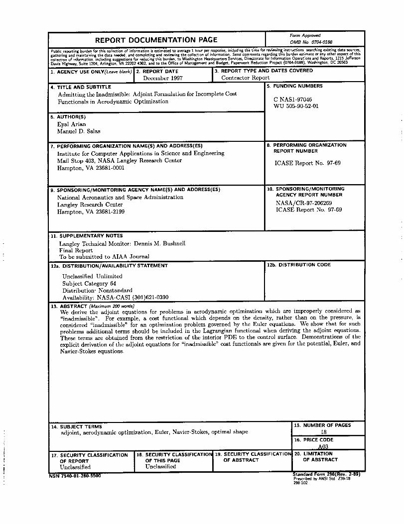
FormApprovedREPORT DOCUMENTATION PAGE OMB No, 0704-0188

Public reporting burden for this collection of information is estimated to average 1 hour per response, including the t_me for rew_vmg._nstructtons: searchmg existing data sources.,

gathering and ma;ntainlng the data needed, and completing and reviewing the collection of information. Send comments regarding this burden estimate or any other aspect of this

coliectlon of information, including suggestions for reducing this burden, to Washington Headquarters Services, Directorate for Informati_on O___ rations a_l Report s_.12_SJetTerson

Davis Highway, Suite 1204, Arlington, VA 22202_,302, and to the Office of" Management and Budget, Paperwork Reduction r'roject (0704-016B), Wasmngton, u_. zu:>ua.

1. AGENCY USE ONLY(Leave blank) 2. REPORT DATE 3. REPORT TYPE AND DATES COVEREDDecember 1997 Contractor Report

4,

6,

7,

TITLE AND SUBTITLE

Admitting the Inadmissible: Adjoint Formulation for Incomplete Cost

Functionals in Aerodynamic Optimization

AUTHOR(S)

Eyal Arian

Manuel D. Salas

PERFORMING ORGANIZATION NAME(S) AND ADDRESS(ES)

Institute for Computer Applications in Science and Engineering

Mail Stop 403, NASA Langley Research Center

Hampton, VA 23681-000I

9. SPONSORING/MONITORING AGENCY NAME(S) AND ADDRESS(ES)

National Aeronautics and Space Administration

Langley Research Center

Hampton, VA 23681-2199

5. FUNDING NUMBERS

C NAS1-97046

WU 505-90-52-01

8. PERFORMING ORGANIZATIONREPORT NUMBER

ICASE Report No. 97-69

10. SPONSORING/MONITORINGAGENCY REPORT NUMBER

NASA/CR-97-206269ICASE Report No. 97-69

11. SUPPLEMENTARY NOTES

Langley Technical Monitor: Dennis M. Bushnell

Final ReportTo be submitted to AIAA Journal

12a. DISTRIBUTION/AVAILABILITY STATEMENT

Unclassified-Unlimited

Subject Category 64Distribution: Nonstandard

Availability: NASA-CASI (301)621-0390

12b. DISTRIBUTION CODE

13. ABSTRACT (Maximum 200 words)We derive the adjoint equations for problems in aerodynamic optimization which are improperly considered as

"inadmissible". For example, a cost functional which depends on the density, rather than on the pressure, isconsidered "inadmissible" for an optimization problem governed by the Euler equations. We show that for such

problems additional terms should be included in the Lagrangian functional when deriving the adjoint equations.These terms are obtained from the restriction of the interior PDE to the control surface. Demonstrations of the

explicit derivation of the adjoint equations for "inadmissible" cost functionals are given for the potential, Euler, and

Navier-Stokes equations.

14. SUBJECT TERMSadjoint, aerodynamic optimization, Euler, Navier-Stokes, optimal shape

17, SECURITY CLASSIFICATION 18. SECURITY CLASSIFICATIONOF REPORT OF THIS PAGEUnclassified Unclassified

NSN 7540-01-280-5500

lg. SECURITY CLASSIFICATIONOF ABSTRACT

15. NUMBER OF PAGES18

16. PRICE CODEA03

20. LIMITATIONOF ABSTRACT

Standard Form 298(Rev. 2-89)Prescribed by ANSI Std. Z39-18

298-102


Recommended