ADMM-NN: An Algorithm-Hardware Co-DesignFramework of DNNs Using Alternating Direction

Method of MultipliersAo Ren

∗

Northeastern University

ren.ao@husky.neu.edu

Tianyun Zhang∗

Syracuse University

tzhan120@syr.edu

Shaokai Ye, Jiayu Li

Syracuse University

{sye106,jli221}@syr.edu

Wenyao Xu

SUNY University at Buffalo

wenyaoxu@buffalo.edu

Xuehai Qian

University of Southern California

xuehai.qian@usc.edu

Xue Lin, Yanzhi Wang

Northeastern University

{xue.lin,yanz.wang}@northeastern.edu

AbstractModel compression is an important technique to facilitate

efficient embedded and hardware implementations of deep

neural networks (DNNs). The target is to simultaneously re-

duce the model storage size and accelerate the computation,

with minor effect on accuracy. Two important categories

of DNN model compression techniques are weight pruning

and weight quantization. The former leverages the redun-

dancy in the number of weights, whereas the latter leverages

the redundancy in bit representation of weights. These two

sources of redundancy can be combined, thereby leading

to a higher degree of DNN model compression. However, a

systematic framework of joint weight pruning and quantiza-

tion of DNNs is lacking, thereby limiting the available model

compression ratio. Moreover, the computation reduction,

energy efficiency improvement, and hardware performance

overhead need to be accounted besides simply model size

reduction.

To address these limitations, we present ADMM-NN, the

first algorithm-hardware co-optimization framework of DNNs

using Alternating Direction Method of Multipliers (ADMM),

a powerful technique to solve non-convex optimization prob-

lems with possibly combinatorial constraints. The first part

of ADMM-NN is a systematic, joint framework of DNN

weight pruning and quantization using ADMM. It can be

∗Ao Ren and Tianyun Zhang Contributed equally to this work.

Permission to make digital or hard copies of all or part of this work for

personal or classroom use is granted without fee provided that copies are not

made or distributed for profit or commercial advantage and that copies bear

this notice and the full citation on the first page. Copyrights for components

of this work owned by others than ACMmust be honored. Abstracting with

credit is permitted. To copy otherwise, or republish, to post on servers or to

redistribute to lists, requires prior specific permission and/or a fee. Request

permissions from permissions@acm.org.

ASPLOS ’19, April 13–17, 2019, Providence, RI, USA© 2019 Association for Computing Machinery.

ACM ISBN 978-1-4503-6240-5/19/04. . . $15.00

https://doi.org/10.1145/3297858.3304076

understood as a smart regularization technique with regular-

ization target dynamically updated in each ADMM iteration,

thereby resulting in higher performance in model compres-

sion than the state-of-the-art. The second part is hardware-

aware DNN optimizations to facilitate hardware-level im-

plementations. We perform ADMM-based weight pruning

and quantization considering (i) the computation reduction

and energy efficiency improvement, and (ii) the hardware

performance overhead due to irregular sparsity. The first

requirement prioritizes the convolutional layer compression

over fully-connected layers, while the latter requires a con-

cept of the break-even pruning ratio, defined as theminimum

pruning ratio of a specific layer that results in no hardware

performance degradation.

Without accuracy loss, ADMM-NN achieves 85× and 24×

pruning on LeNet-5 and AlexNet models, respectively, — sig-

nificantly higher than the state-of-the-art. Combiningweight

pruning and quantization, we achieve 1,910× and 231× reduc-

tions in overall model size on these two benchmarks . Highly

promising results are also observed on other representative

DNNs such as VGGNet and ResNet-50. We release codes and

models at https://github.com/yeshaokai/admm-nn.

CCS Concepts • Computing methodologies→Neuralnetworks; Regularization; •Hardware→ Application-specific VLSI designs.

Keywords Neural Network, ADMM,Weight Pruning, Quan-

tization, Hardware Optimization

ACM Reference Format:Ao Ren, Tianyun Zhang, Shaokai Ye, Jiayu Li, Wenyao Xu, Xuehai

Qian, and Xue Lin, Yanzhi Wang. 2019. ADMM-NN: An Algorithm-

Hardware Co-Design Framework of DNNs Using Alternating Di-

rection Method of Multipliers. In 2019 Architectural Support forProgramming Languages and Operating Systems (ASPLOS ’19), April13–17, 2019, Providence, RI, USA.ACM, New York, NY, USA, 14 pages.

https://doi.org/10.1145/3297858.3304076

1 IntroductionThe wide applications of deep neural networks (DNNs), es-

pecially for embedded and IoT systems, call for efficient

implementations of (at least) the inference phase of DNNs

in power-budgeted systems. To achieve both high perfor-

mance and energy efficiency, hardware acceleration of DNNs,including both FPGA-based and ASIC-based implementa-

tions, has been intensively studied both in academia and

industry [1, 2, 4, 6–8, 13, 16, 20, 21, 28, 31, 35, 37, 41, 43–

45, 48, 49, 51, 52, 54, 61, 62, 65]. With large model size (e.g.,

for ImageNet dataset [11]), hardware accelerators suffer from

the frequent access to off-chip DRAM due to the limited on-

chip SRAMmemory. Unfortunately, off-chip DRAM accesses

consume significant energy, e.g., 200× compared to on-chip

SRAM [8, 21], and can thus easily dominate the whole system

power consumption.

To overcome this hurdle, a number of prior work are dedi-

cated to model compression techniques for DNNs, in order to

simultaneously reduce the model size, i.e., storage require-

ment, and accelerate the computation, with minor effect on

accuracy. Two important categories of DNN model compres-

sion techniques are weight pruning and weight quantization.A pioneering work of weight pruning is Han et al. [24],

which is an iterative, heuristic method and achieves 9× reduc-

tion in the number of weights in AlexNet (ImageNet dataset).

This work has been extended for improving the weight prun-

ing ratio and actual implementation efficiency [18, 20, 21].

Weight quantization of DNNs has also been investigated

in plenty of recent work [9, 27, 33, 34, 40, 42, 55, 57, 66],

quantizing DNN weights to binary values, ternary values, or

powers of 2, with acceptable accuracy loss. In this manner,

both storage and computational requirements are reduced.

Multiplication operations may even be eliminated through

binary or ternary weight quantizations [9, 27, 42].

The effectiveness of weight pruning lies on the redun-

dancy in the number of weights in DNN, whereas the effec-

tiveness of weight quantization is due to the redundancy in

bit representation of weights. Ideally, these two sources of

redundancy can be combined, thereby leading to a higher de-

gree of DNN model compression. Despite certain prior work

investigating in this aspect using greedy, heuristic method

[21, 22, 66], a systematic framework of joint weight pruning

and quantization of DNNs is still lacking. As a result, they

cannot achieve the highest possible model compression ratio

by fully exploiting the degree of redundancy.

Moreover, the prior work on weight pruning and quan-

tization mainly focus on reducing the model size of DNNs.As a result, the major model compression is achieved in the

fully-connected (FC) layers, which exhibit higher degree of

redundancy. On the other hand, the convolutional (CONV)

layers, which are the most computationally intensive part

of DNNs, do not achieve a significant gain in compression.

For example, the pioneering work [24] achieves only 2.7×

weight reduction in CONV layers for AlexNet model, which

still leaves a high improvement margin if the focus is on

computation reductions. Furthermore, the weight pruning

technique incurs irregularity in weight storage, i.e., the irreg-ular sparsity, and corresponding overheads in index storage

and calculations, parallelism degradation, etc. These over-

heads pose important challenges in hardware implementa-

tions. Take [24] as an example, the 2.7× weight reduction

in CONV layers often results in performance degradationsas observed in multiple actual hardware implementations

[20, 53, 56, 58].

To address the above limitations, this paper presents ADMM-

NN, the first algorithm-hardware co-design framework of

DNNs usingAlternating DirectionMethod ofMultipliers (ADMM),— a powerful technique to deal with non-convex optimization

problems with possibly combinatorial constraints [5, 38, 50].

The ADMM-NN framework is general, with applications at

software-level, FPGA, ASIC, or in combination with new

devices and hardware advances.

The first part of ADMM-NN is a systematic, joint frame-

work of DNNweight pruning and quantization using ADMM.

Through the application of ADMM, the weight pruning and

quantization problems are decomposed into two subprob-

lems: The first is minimizing the loss function of the original

DNN with an additional L2 regularization term, and can be

solved using standard stochastic gradient descent like ADAM

[29]. The second one can be optimally and analytically solved

[5]. The ADMM framework can be understood as a smart

regularization technique with regularization target dynami-

cally updated in each ADMM iteration, thereby resulting in

high performance in model compression.

The second part of ADMM-NN is hardware-aware op-

timization of DNNs to facilitate efficient hardware imple-

mentations. Specifically, we perform ADMM-based weight

pruning and quantization accounting for (i) the computation

reduction and energy efficiency improvement, and (ii) the

hardware performance overhead due to irregular sparsity.

We mainly focus on the model compression on CONV lay-

ers, but the FC layers need to be compressed accordingly in

order to avoid overfitting (and accuracy degradation). We

adopt a concept of the break-even pruning ratio, defined as

the minimum weight pruning ratio of a specific DNN layer

that will not result in hardware performance (speed) degra-

dation. These values are hardware platform-specific. Based

on the calculation of such ratios through hardware synthe-

sis (accounting for the hardware performance overheads),

we develop efficient DNN model compression algorithm for

computation reduction and hardware implementations.

In summary, the contributions of this paper include: (i)

ADMM-based weight pruning and weight quantization for

DNNs; (ii) a systematic, joint framework for DNNmodel com-

pression; and (iii) hardware-aware DNN model compression

for computation reduction and efficiency improvement.

Figure 1. Illustration of weight pruning for DNNs.

Experimental results demonstrate the effectiveness of the

proposed ADMM-NN framework. Without any accuracy

loss, ADMM-NN can achieve 85× and 24× weight pruning

on LeNet-5 and AlexNet models, respectively, which are

significantly higher than the state-of-the-art iterative prun-

ing [] (12× and 9×, respectively). With the focus on data

storage, weight pruning and weight quantization can be

combined, ADMM-NN achieves 1,910× and 231× reductions

in overall model size on these two benchmarks, respectively.

Promising results are also observed on other representa-

tive DNNs such as VGGNet and ResNet-50. The computa-

tion reduction is even more significant compared with prior

work. Without any accuracy loss, we can achieve 3.6× re-

duction in the amount of computation compared with the

state-of-the-art [22, 24]. We release codes and models at:

https://github.com/yeshaokai/admm-nn.

2 Background2.1 Related Work on Weight Pruning and

QuantizationWeight pruningmethods leverage the inherent redundancy

in the number of weights in DNNs, thereby achieving effec-

tive model compression with negligible accuracy loss, as

illustrated in Fig. 1. A pioneering work of weight pruning is

[24]. It uses a heuristic, iterative method to prune the weights

with small magnitudes and retrain the DNN. It achieves 9×

weight reduction on AlexNet for ImageNet dataset, without

accuracy degradation. However, this original work achieves

relatively low compression ratio (2.7× for AlexNet) on the

CONV layers, which are the key computational part in state-

of-the-art DNNs [25, 47]. Besides, indices are needed, at

least one per weight, to index the relative location of the

next weight. As a result, it suffers from low performance im-

provement (sometimes even degradation) in actual hardware

implementations [53, 56, 58], when the overhead of irregular

sparsity is accounted for.

This work has been extended in two directions. The first

is improving the weight reduction ratio by using more so-

phisticated heuristics, e.g., incorporating both weight prun-

ing and growing [19], using L1 regularization method [53],

or genetic algorithm [10]. As an example, the recent work

NeST [10] achieves 15.7× weight reduction on AlexNet with

zero accuracy loss, at the cost of significant training over-

head. The second is enhancing the actual implementation

efficiency. This goal is achieved by either deriving an effec-

tive tradeoff between accuracy and compression ratio, e.g.,

the energy-aware pruning [56], or incorporating regularity

and structures into the weight pruning framework, e.g., the

channel pruning [26] and structured sparsity learning [53]

approaches.

Weight quantization methods leverage the inherent re-

dundancy in the number of bits for weight representation.

Many relatedwork [9, 27, 33, 34, 40, 42, 55, 66] present weight

quantization techniques to binary values, ternary values, or

powers of 2 to facilitate hardware implementations, with ac-

ceptable accuracy loss. The state-of-the-art technique adopts

an iterative quantization and retraining framework, with

randomness incorporated in quantization [9]. It achieves

less than 3% accuracy loss on AlexNet for binary weight

quantization [33]. It is also worth noticing that a similar

technique, weight clustering, groups weights into clusters

with arbitrary values. This is different from equal-interval

values as in quantization. As a result weight clustering is not

as hardware-friendly as quantization [22, 67].

Pros and cons of the two methods: Weight quantiza-

tion has clear advantage: it is hardware-friendly. The com-

putation requirement is reduced in proportion to weight

representation, and multiplication operations can be elimi-

nated using binary/ternary quantizations. On the other hand,

weight pruning incurs inevitable implementation overhead

due to the irregular sparsity and indexing [14, 22, 53, 56, 58].

The major advantage of weight pruning is the higher

potential gain in model compression. The reasons are two

folds. First, there is often higher degree of redundancy in the

number of weights than bit representation. In fact, reduc-

ing each bit in weight presentation doubles the imprecision,

which is not the case in pruning. Second, weight pruning

performs regularization that strengthens the salient weights

and prunes the unimportant ones. It can even increase the

accuracy with a moderate pruning ratio [23, 53]. As a result

it provides a higher margin of weight reduction. This effect

does not exist in weight quantization/clustering.

Combination: Because they leverage different sources

of redundancy, weight pruning and quantization can be ef-

fectively combined. However, there lacks a systematic inves-

tigation in this direction. The extended work [22] by Han etal. uses a combination of weight pruning and clustering (not

quantization) techniques, achieving 27× model compression

on AlexNet. This compression ratio has been updated by

the recent work [66] to 53× on AlexNet (but without any

specification about compressed model).

2.2 Basics of ADMMADMM has been demonstrated [38, 50] as a powerful tool

for solving non-convex optimization problems, potentially

with combinatorial constraints. Consider a non-convex opti-

mization problem that is difficult to solve directly. ADMM

method decomposes it into two subproblems that can be

solved separately and efficiently. For example, the optimiza-

tion problem

min

xf (x) + д(x) (1)

lends itself to the application of ADMM if f (x) is differen-tiable and д(x) has some structure that can be exploited. Ex-

amples of д(x) include the L1-norm or the indicator function

of a constraint set. The problem is first re-written as

min

x,zf (x) + д(z),

subject to x = z.(2)

Next, by using augmented Lagrangian [5], the above prob-

lem is decomposed into two subproblems on x and z. Thefirst isminx f (x)+q1(x), where q1(x) is a quadratic function.As q1(x) is convex, the complexity of solving subproblem 1

(e.g., via stochastic gradient descent) is the same as minimiz-

ing f (x). Subproblem 2 is minz д(z) + q2(z), where q2(z) is aquadratic function. When function д has some special struc-

ture, exploiting the properties of д allows this problem to be

solved analytically and optimally. In this way we can get rid

of the combinatorial constraints and solve the problem that

is difficult to solve directly.

3 ADMM Framework for Joint WeightPruning and Quantization

In this section, we present the novel framework of ADMM-

based DNN weight pruning and quantization, as well as the

joint model compression problem.

3.1 Problem FormulationConsider a DNN with N layers, which can be convolutional

(CONV) and fully-connected (FC) layers. The collection of

weights in the i-th layer isWi ; the collection of bias in the

i-th layer is denoted by bi . The loss function associated with

the DNN is denoted by f({Wi }

Ni=1, {bi }

Ni=1

).

The problem of weight pruning and quantization is an

optimization problem [57, 64]:

minimize

{Wi }, {bi }f({Wi }

Ni=1, {bi }

Ni=1

),

subject to Wi ∈ Si , i = 1, . . . ,N .(3)

Thanks to the flexibility in the definition of the constraint

set Si , the above formulation is applicable to the individ-

ual problems of weight pruning and weight quantization, as

well as the joint problem. For the weight pruning problem,

the constraint set Si = {the number of nonzero weights is

less than or equal to αi }, where αi is the desired number of

weights after pruning in layer i1. For the weight quantiza-tion problem, the set Si={the weights in layer i are mapped

1An alternative formulation is to use a single α as an overall constraint on

the number of weights in the whole DNN.

to the quantization values} {Q1,Q2, · · · ,QM }}, where M is

the number of quantization values/levels. For quantization,

these Q values are fixed, and the interval between two near-

est quantization values is the same, in order to facilitate

hardware implementations.

For the joint problem, the above two constraints need to

be satisfied simultaneously. That is, the number of nonzero

weights should be less than or equal to αi in each layer, whilethe remaining nonzero weights should be quantized.

3.2 ADMM-based Solution FrameworkThe above problem is non-convex with combinatorial con-

straints, and cannot be solved using stochastic gradient de-scent methods (e.g., ADAM [29]) as in original DNN train-

ing. But it can be efficiently solved using the ADMM frame-

work (combinatorial constraints can be get rid of.) To apply

ADMM, we define indicator functions

дi (Wi ) =

{0 if Wi ∈ Si ,+∞ otherwise,

for i = 1, . . . ,N . We then incorporate auxiliary variables Ziand rewrite problem (3) as

minimize

{Wi }, {bi }f({Wi }

Ni=1, {bi }

Ni=1

)+

N∑i=1

дi (Zi ),

subject to Wi = Zi , i = 1, . . . ,N .

(4)

Through application of the augmented Lagrangian [5],

problem (4) is decomposed into two subproblems by ADMM.

We solve the subproblems iteratively until convergence. The

first subproblem is

minimize

{Wi }, {bi }f({Wi }

Ni=1, {bi }

Ni=1

)+

N∑i=1

ρi2

∥Wi − Zki + Uki ∥

2

F ,

(5)

where Uki is the dual variable updated in each iteration,

Uki := Uk−1

i +Wki − Zki . In the objective function of (5), the

first term is the differentiable loss function of DNN, and the

second quadratic term is differentiable and convex. The com-

binatorial constraints are effectively get rid of. This problem

can be solved by stochastic gradient descent (e.g., ADAM)

and the complexity is the same as training the original DNN.

The second subproblem is

minimize

{Zi }

N∑i=1

дi (Zi ) +N∑i=1

ρi2

∥Wk+1i − Zi + Uk

i ∥2

F . (6)

As дi (·) is the indicator function of Si , the analytical solutionof subproblem (6) is

Zk+1i = ΠSi (Wk+1i + Uk

i ), (7)

whereΠSi (·) is Euclidean projection ofWk+1i +U

ki onto the set

Si . The details of the solution to this subproblem is problem-

specific. For weight pruning and quantization problems, the

optimal, analytical solutions of this problem can be found.

Weight Pruning:Formulate as prob. (4);

Subprob. 1:Given Zi, optimize Wi;

Subprob. 2:Given Wi, optimize Zi by setting sparsity;

Subprob. 1:Given Zi, optimize Wi;

Subprob. 2:Given Wi, optimize Zi by mapping to quant. values;

Weight Quantization:Formulate as prob. (4);

Figure 2. Algorithm of joint weight pruning and quantiza-

tion using ADMM.

The derived Zk+1i will be fed into the first subproblem in the

next iteration.

The intuition of ADMM is as follows. In the context of

DNNs, the ADMM-based framework can be understood as

a smart regularization technique. Subproblem 1 (Eqn. (5))

performs DNN training with an additional L2 regularizationterm, and the regularization target Zki − Uk

i is dynamically

updated in each iteration through solving subproblem 2. This

dynamic updating process is the key reason why ADMM-

based framework outperforms conventional regularization

method in DNN weight pruning and quantization.

3.3 Solution to Weight Pruning and Quantization,and the Joint Problem

Both weight pruning and quantization problems can be ef-

fectively solved using the ADMM framework. For the weight

pruning problem, the Euclidean projection Eqn. (7) is to keep

αi elements in Wk+1i + Uk

i with largest magnitude and set

the rest to be zero [38, 50]. This is proved to be the optimal

and analytical solution to subproblem 2 (Eqn. (6)) in weight

pruning.

For the weight quantization problem, the Euclidean pro-

jection Eqn. (7) is to set every element in Wk+1i + Uk

i to be

the quantization value closest to that element. This is also

the optimal and analytical solution to subproblem 2 in quan-

tization. The determination of quantization values will be

discussed in details in the next subsection.

For both weight pruning and quantization problems, the

first subproblem has the same form when Zki is determined

through Euclidean projection. As a result they can be solved

in the same way by stochastic gradient descent (e.g., the

ADAM algorithm).

For the joint problem of weight pruning and quantization,

there is an additional degree of flexibility when perform-

ing Euclidean projection, i.e., a specific weight can be either

projected to zero or to a closest quantization value. This flex-

ibility will add difficulty in optimization. To overcome this

hurdle, we perform weight pruning and quantization in two

steps. We choose to perform weight pruning first, and then

implement weight quantization on the remaining, non-zero

weights. The reason for this order is the following observa-

tion: There typically exists higher degree of redundancy in

the number of weights than the bit representation of weights.

As a result, we can typically achieve higher model compres-

sion degree using weight pruning, without any accuracy loss,

compared with quantization. The observation is validated

by prior work [18, 20, 21] (although many are on clustering

instead of quantization), and in our own investigations. Fig. 2

summaries the key steps of solving the joint weight pruning

and quantization problem based on ADMM framework.

Thanks to the fast theoretical convergence rate of ADMM,

the proposed algorithms have fast convergence. To achieve

a good enough compression ratio for AlexNet, we need 72

hours for weight pruning and 24 hours for quantization. This

is much faster than [24] that requires 173 hours for weight

pruning only.

3.4 Details in Parameter Determination3.4.1 Determination of Weight Numbers in Pruning:The most important parameters in the ADMM-based weight

pruning step are the αi values for each layer i . To determine

these values, we start from the values derived from the prior

weight pruning work [22, 24]. When targeting high compres-

sion ratio, we reduce the αi values proportionally for each

layer.When targeting computation reductions, we deduct the

αi values for convolutional (CONV) layers, because CONVlayers account for the major computation compared with

FC layers. Our experimental results demonstrate about 2-3×

further compression under the same accuracy, compared

with the prior work [15, 22, 24, 59].

The additional parameters in ADMM-based weight prun-

ing, i.e., the penalty parameters ρi , are set to be ρ1 = · · · =

ρN = 3×10−3. This choice is basically very close for different

DNN models, such as AlexNet [30] and VGG-16 [46]. The

pruning results are not sensitive to the penalty parameters

of the optimal choice, unless these parameters are increased

or decreased by orders of magnitude.

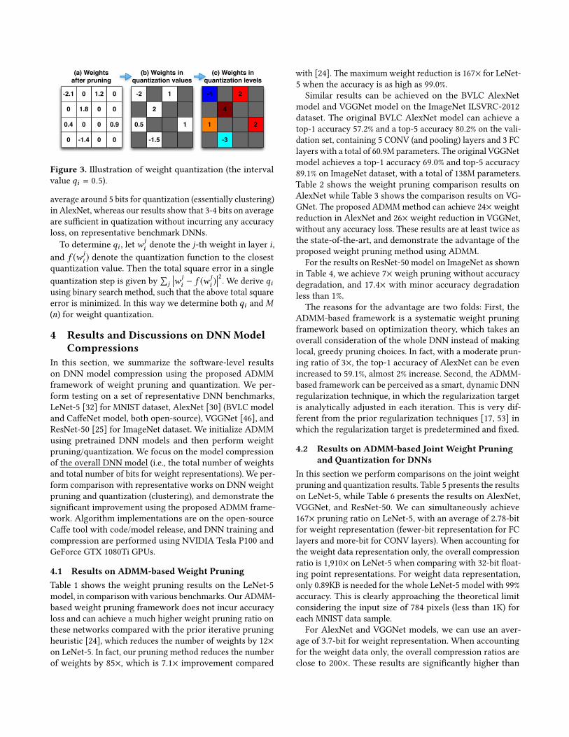
3.4.2 Determination of Quantization Values:After weight pruning is performed, the next step is weight

quantization on the remaining, non-zero weights. We use

n bits for equal-distance quantization to facilitate hardware

implementations, which means there are a total of M =

2nquantization levels. More specifically, for each layer i ,

we quantize the weights into a set of quantization values

{−M

2

qi , ...,−2qi ,−qi ,qi , 2qi , ...,M

2

qi }. Please note that 0 is

not a quantization value because it means that the corre-

sponding weight has been pruned.

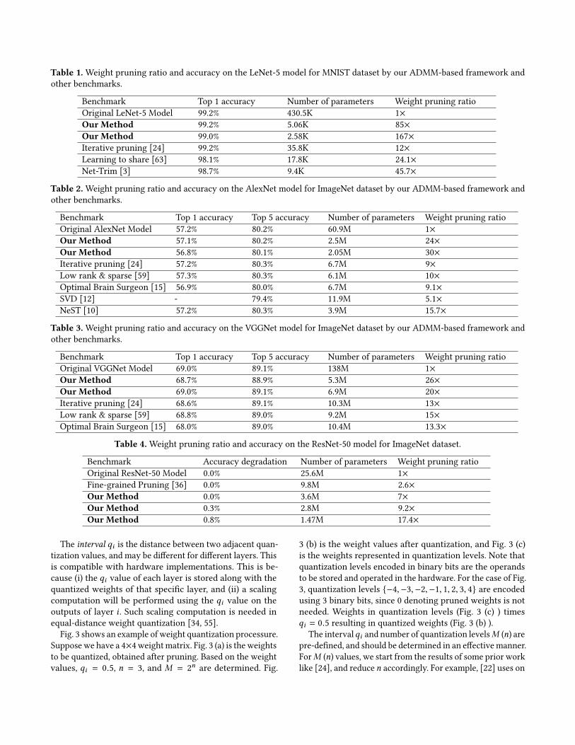
Table 1.Weight pruning ratio and accuracy on the LeNet-5 model for MNIST dataset by our ADMM-based framework and

other benchmarks.

Benchmark Top 1 accuracy Number of parameters Weight pruning ratio

Original LeNet-5 Model 99.2% 430.5K 1×

Our Method 99.2% 5.06K 85×

Our Method 99.0% 2.58K 167×

Iterative pruning [24] 99.2% 35.8K 12×

Learning to share [63] 98.1% 17.8K 24.1×

Net-Trim [3] 98.7% 9.4K 45.7×

Table 2. Weight pruning ratio and accuracy on the AlexNet model for ImageNet dataset by our ADMM-based framework and

other benchmarks.

Benchmark Top 1 accuracy Top 5 accuracy Number of parameters Weight pruning ratio

Original AlexNet Model 57.2% 80.2% 60.9M 1×

Our Method 57.1% 80.2% 2.5M 24×

Our Method 56.8% 80.1% 2.05M 30×

Iterative pruning [24] 57.2% 80.3% 6.7M 9×

Low rank & sparse [59] 57.3% 80.3% 6.1M 10×

Optimal Brain Surgeon [15] 56.9% 80.0% 6.7M 9.1×

SVD [12] - 79.4% 11.9M 5.1×

NeST [10] 57.2% 80.3% 3.9M 15.7×

Table 3. Weight pruning ratio and accuracy on the VGGNet model for ImageNet dataset by our ADMM-based framework and

other benchmarks.

Benchmark Top 1 accuracy Top 5 accuracy Number of parameters Weight pruning ratio

Original VGGNet Model 69.0% 89.1% 138M 1×

Our Method 68.7% 88.9% 5.3M 26×

Our Method 69.0% 89.1% 6.9M 20×

Iterative pruning [24] 68.6% 89.1% 10.3M 13×

Low rank & sparse [59] 68.8% 89.0% 9.2M 15×

Optimal Brain Surgeon [15] 68.0% 89.0% 10.4M 13.3×

Table 4. Weight pruning ratio and accuracy on the ResNet-50 model for ImageNet dataset.

Benchmark Accuracy degradation Number of parameters Weight pruning ratio

Original ResNet-50 Model 0.0% 25.6M 1×

Fine-grained Pruning [36] 0.0% 9.8M 2.6×

Our Method 0.0% 3.6M 7×

Our Method 0.3% 2.8M 9.2×

Our Method 0.8% 1.47M 17.4×

The interval qi is the distance between two adjacent quan-

tization values, and may be different for different layers. This

is compatible with hardware implementations. This is be-

cause (i) the qi value of each layer is stored along with the

quantized weights of that specific layer, and (ii) a scaling

computation will be performed using the qi value on the

outputs of layer i . Such scaling computation is needed in

equal-distance weight quantization [34, 55].

Fig. 3 shows an example of weight quantization processure.

Supposewe have a 4×4weightmatrix. Fig. 3 (a) is theweights

to be quantized, obtained after pruning. Based on the weight

values, qi = 0.5, n = 3, and M = 2nare determined. Fig.

3 (b) is the weight values after quantization, and Fig. 3 (c)

is the weights represented in quantization levels. Note that

quantization levels encoded in binary bits are the operands

to be stored and operated in the hardware. For the case of Fig.

3, quantization levels {−4,−3,−2,−1, 1, 2, 3, 4} are encodedusing 3 binary bits, since 0 denoting pruned weights is not

needed. Weights in quantization levels (Fig. 3 (c) ) times

qi = 0.5 resulting in quantized weights (Fig. 3 (b) ).

The intervalqi and number of quantization levelsM (n) arepre-defined, and should be determined in an effectivemanner.

ForM (n) values, we start from the results of some prior work

like [24], and reduce n accordingly. For example, [22] uses on

-2.1 0 1.2 0

0 1.8 0 0

0.4 0 0 0.9

0 -1.4 0 0

-2 1

2

0.5 1

-1.5

-4 2

4

1 2

-3

(a) Weights after pruning

(b) Weights inquantization values

(c) Weights inquantization levels

Figure 3. Illustration of weight quantization (the interval

value qi = 0.5).

average around 5 bits for quantization (essentially clustering)

in AlexNet, whereas our results show that 3-4 bits on average

are sufficient in quatization without incurring any accuracy

loss, on representative benchmark DNNs.

To determine qi , letwji denote the j-th weight in layer i ,

and f (w ji ) denote the quantization function to the closest

quantization value. Then the total square error in a single

quantization step is given by

∑j��w j

i − f (w ji )��2. We derive qi

using binary search method, such that the above total square

error is minimized. In this way we determine both qi andM(n) for weight quantization.

4 Results and Discussions on DNN ModelCompressions

In this section, we summarize the software-level results

on DNN model compression using the proposed ADMM

framework of weight pruning and quantization. We per-

form testing on a set of representative DNN benchmarks,

LeNet-5 [32] for MNIST dataset, AlexNet [30] (BVLC model

and CaffeNet model, both open-source), VGGNet [46], and

ResNet-50 [25] for ImageNet dataset. We initialize ADMM

using pretrained DNN models and then perform weight

pruning/quantization. We focus on the model compression

of the overall DNN model (i.e., the total number of weights

and total number of bits for weight representations). We per-

form comparison with representative works on DNN weight

pruning and quantization (clustering), and demonstrate the

significant improvement using the proposed ADMM frame-

work. Algorithm implementations are on the open-source

Caffe tool with code/model release, and DNN training and

compression are performed using NVIDIA Tesla P100 and

GeForce GTX 1080Ti GPUs.

4.1 Results on ADMM-based Weight PruningTable 1 shows the weight pruning results on the LeNet-5

model, in comparison with various benchmarks. Our ADMM-

based weight pruning framework does not incur accuracy

loss and can achieve a much higher weight pruning ratio on

these networks compared with the prior iterative pruning

heuristic [24], which reduces the number of weights by 12×

on LeNet-5. In fact, our pruning method reduces the number

of weights by 85×, which is 7.1× improvement compared

with [24]. The maximum weight reduction is 167× for LeNet-

5 when the accuracy is as high as 99.0%.

Similar results can be achieved on the BVLC AlexNet

model and VGGNet model on the ImageNet ILSVRC-2012

dataset. The original BVLC AlexNet model can achieve a

top-1 accuracy 57.2% and a top-5 accuracy 80.2% on the vali-

dation set, containing 5 CONV (and pooling) layers and 3 FC

layers with a total of 60.9M parameters. The original VGGNet

model achieves a top-1 accuracy 69.0% and top-5 accuracy

89.1% on ImageNet dataset, with a total of 138M parameters.

Table 2 shows the weight pruning comparison results on

AlexNet while Table 3 shows the comparison results on VG-

GNet. The proposed ADMMmethod can achieve 24× weight

reduction in AlexNet and 26× weight reduction in VGGNet,

without any accuracy loss. These results are at least twice as

the state-of-the-art, and demonstrate the advantage of the

proposed weight pruning method using ADMM.

For the results on ResNet-50 model on ImageNet as shown

in Table 4, we achieve 7× weigh pruning without accuracy

degradation, and 17.4× with minor accuracy degradation

less than 1%.

The reasons for the advantage are two folds: First, the

ADMM-based framework is a systematic weight pruning

framework based on optimization theory, which takes an

overall consideration of the whole DNN instead of making

local, greedy pruning choices. In fact, with a moderate prun-

ing ratio of 3×, the top-1 accuracy of AlexNet can be even

increased to 59.1%, almost 2% increase. Second, the ADMM-

based framework can be perceived as a smart, dynamic DNN

regularization technique, in which the regularization target

is analytically adjusted in each iteration. This is very dif-

ferent from the prior regularization techniques [17, 53] in

which the regularization target is predetermined and fixed.

4.2 Results on ADMM-based Joint Weight Pruningand Quantization for DNNs

In this section we perform comparisons on the joint weight

pruning and quantization results. Table 5 presents the results

on LeNet-5, while Table 6 presents the results on AlexNet,

VGGNet, and ResNet-50. We can simultaneously achieve

167× pruning ratio on LeNet-5, with an average of 2.78-bit

for weight representation (fewer-bit representation for FC

layers and more-bit for CONV layers). When accounting for

the weight data representation only, the overall compression

ratio is 1,910× on LeNet-5 when comparing with 32-bit float-

ing point representations. For weight data representation,

only 0.89KB is needed for the whole LeNet-5 model with 99%

accuracy. This is clearly approaching the theoretical limit

considering the input size of 784 pixels (less than 1K) for

each MNIST data sample.

For AlexNet and VGGNet models, we can use an aver-

age of 3.7-bit for weight representation. When accounting

for the weight data only, the overall compression ratios are

close to 200×. These results are significantly higher than

Table 5.Model size compression ratio on the LeNet-5 model for MNIST dataset by our ADMM-based framework and baseline.

Benchmark Accuracy

degrade

Para. No. CONV

quant.

FC

quant.

Total data size/

Compress ratio

Total model size

(including index)/

Compress ratio

Original LeNet-5 0.0% 430.5K 32b 32b 1.7MB 1.7MB

Our Method 0.2% 2.57K 3b 2b 0.89KB / 1,910× 2.73KB / 623×

Iterative pruning [22] 0.1% 35.8K 8b 5b 24.2KB / 70.2× 52.1KB / 33×

Table 6. Model size compression ratio on the AlexNet, VGGNet, and ResNet-50 models for ImageNet dataset by our ADMM-

based framework and baselines.

Benchmark Accuracy

degrade

Para. No. CONV

quant.

FC

quant.

Total data size/

Compress ratio

Total model size

(including index)/

Compress ratio

Original AlexNet 0.0% 60.9M 32b 32b 243.6MB 243.6MB

Our Method 0.2% 2.25M 5b 3b 1.06MB / 231 × 2.45MB / 99×

Iterative pruning [22] 0.0% 6.7M 8b 5b 5.4MB / 45× 9.0MB / 27×

Binary quant. [33] 3.0% 60.9M 1b 1b 7.3MB / 32× 7.3MB / 32×

Ternary quant. [33] 1.8% 60.9M 2b 2b 15.2MB / 16× 15.2MB / 16×

Original VGGNet 0.0% 138M 32b 32b 552MB 552MB

Our Method 0.1% 6.9M 5b 3b 3.2MB / 173× 8.3MB / 66.5×

Iterative pruning [22] 0.0% 10.3M 8b 5b 8.2MB / 67× 17.8MB / 31×

Binary quant. [33] 2.2% 138M 1b 1b 17.3MB / 32× 17.3MB / 32×

Ternary quant. [33] 1.1% 138M 2b 2b 34.5MB / 16× 34.5MB / 16×

Original ResNet-50 0.0% 25.6M 32b 32b 102.4MB 102.4MB

Our Method 0.0% 3.6M 6b 6b 2.7MB / 38× 4.1MB / 25.3×

Our Method 2.0% 1.47M 4b 4b 0.73MB / 140× 1.65MB / 62×

the prior work such as [22, 24], even when [22] focuses on

weight clustering instead of quantization2. For example, [24]

achieves 9× weight pruning on AlexNet and uses an aver-

age of higher than 5 bits (8 bits for CONV layers and 5 bits

for FC layers) for weight representation. These results are

also higher than performing weight quantization/clustering

alone because the maximum possible gain when performing

quantization/clustering alone is 32 (we need to use 1 bit per

weight anyway) compared with floating-point representa-

tions, let alone accuracy degradations. These results clearly

demonstrate the effectiveness of the proposed ADMM frame-

work on joint weight pruning and quantization for DNNs.

Similar results are also observed on the joint weight pruning

and quantization results on ResNet-50 model.

However, we must emphasize that the actual storage re-

duction cannot reach such a high gain. For DNNs, the modelsize is defined as the total number of bits (or Bytes) to ac-

tually store a DNN model. The reason for this gap is the

indices, which are needed (at least) one per weight with

weight pruning in order to locate the ID of the next weight

[24]. For instance, we need more bits for each index for the

2Weight clustering is less hardware-friendly, but should perform better than

weight quantization in model compression. The reason is because weight

quantization can be perceived as a special case of clustering.

pruned AlexNet than [24] because we achieve a higher prun-

ing ratio. The storage requirement for indices will be even

higher compared with the actual data, because the ADMM

framework is very powerful in weight quantization. This

will add certain overhead for the overall model storage, as

also shown in the tables.

Table 7. Layer-wise weight pruning results on the AlexNet

model without accuracy loss using the ADMM framework.

Layer Para.

No.

Para.

No. after

prune

Para. Percentage

after prune

conv1 34.8K 28.19K 81%

conv2 307.2K 61.44K 20%

conv3 884.7K 168.09K 19%

conv4 663.5K 132.7K 20%

conv5 442.4K 88.48K 20%

fc1 37.7M 1.06M 2.8%

fc2 16.8M 0.99M 5.9%

fc3 4.1M 0.38M 9.3%

total 60.9M 2.9M 4.76%

Finally, we point out that it may be somewhat biased

when only considering the model size reduction of DNNs.

We list in Table 7 the layer-wise weight pruning results for

AlexNet, using the proposed ADMM framework. We can

observe that the major weight pruning and quantization are

achieved in the FC layers, compared with CONV layers. The

reasons are that the FC layers account for more than 90% of

weights and possess a higher degree of redundancy, thereby

enabling higher degree of weight pruning/quantization. This

is the same as the prior work such as [24], which achieves 9×

overall weight reduction while only 2.7× reduction on CONV

layers. On the other hand, we emphasize that the CONV

layers account for the major computation in state-of-the-art

DNNs, e.g., 95% to 98% in AlexNet and VGGNet [30, 46], and

even more for ResNet [25]. For computation reduction and

energy efficiency improvement, it is more desirable to focus

on CONV layers for weight pruning and quantization. This

aspect will be addressed in the next section.

4.3 Making AlexNet and VGGNet On-ChipAn important indication of the proposed ADMM framework

is that the weights of most of the large-scale DNNs can be

stored on-chip for FPGA and ASIC designs. Let us consider

AlexNet and VGGNet as examples. For AlexNet, the num-

ber of weights before pruning is 60.9M, corresponding to

244MB storage (model size) when 32-bit floating point num-

ber is utilized for weight representation. Using the proposed

ADMM weight pruning and quantization framework, the

total storage (model size) of AlexNet is reduced to 2.45MB

(using 2.25M weights) when the indices are accounted for.

This model size is easily accommodated by the medium-to-

high end FPGAs, such as Xilinx Kintex-7 series, and ASIC

designs. This is achieved without any accuracy loss.

On the other hand, VGGNet, as one of the largest DNNs

that is widely utilized, has a total number of 138M weights,

corresponding to 552MB storage when 32-bit floating point

number is used for weight representation. Using the pro-

posed ADMM framework, the total model size of VGGNet is

reduced to 8.3MB (using 6.9M weights) when the indices are

accounted for. This model size can still be accommodated

by a single high-end FPGA such as Altera (Intel) DE-5 and

Xilinx Virtex-7. The effect that large-scale AlexNet and VG-

GNet models can be stored using on-chip memory of single

FPGA/ASIC will significantly facilitate the wide application

of large-scale DNNs, in embedded, mobile, and IoT systems.

It can be a potential game changer. On the other hand, when

accounting for the computation reductions rather than mere

storage (model size) reduction, it is more desirable to focus

mainly on the model compression on CONV layers rather

than the whole DNN model. Also it is desirable to focus

more on CONV layers since a smaller on-chip memory can

be both cost and speed-beneficial, which is critical especially

for custom ASIC.

5 Hardware-Aware ComputationReduction

Motivation As discussed in the previous section and illus-

trated in Table 7, the current gains in weight pruning and

quantization are mainly attributed to the redundancy in FC

layers. This optimization target is not the most desirable

when accounting for the computation reduction and energy

efficiency improvement. The reason is that CONV layers

account for the major computation in state-of-the-art DNNs,

even reaching 98% to 99% for the recent VGGNet and ResNet

models [30, 46]. In actual ASIC design and implementations,

it will be desirable to allocate on-chip memory for the com-

pressed CONV layers while using off-chip memory for the

less computationally intensive FC layers. In this way the on-

chip memory can be reduced, while the major computation

part of DNN (CONV layers) can be accelerated. Therefore

it is suggested to perform weight pruning and quantization

focusing on the CONV layers.

The prior weight pruning work [22, 24] cannot achieve

a satisfactory weight pruning ratio on CONV layers while

guaranteeing the overall accuracy. For example, [24] achieves

only 2.7×weight pruning on the CONV layers of AlexNet. In

fact, the highest gain in reference work on CONV layer prun-

ing is 5.0× using L1 regularization [53], and does not performany pruning on FC layers. Sometimes, a low weight pruning

ratio will result in hardware performance degradation, as

reported in a number of actual hardware implementations

[53, 56, 58]. The key reason is the irregularity in weight stor-

age, the associated overhead in calculating weight indices,

and the degradation in parallelism. This overhead is encoun-

tered in the PE (processing element) design when sparsity

(weight pruning) is utilized. This overhead needs to be ac-

curately characterized and effectively accounted for in the

hardware-aware weight pruning framework.

5.1 Algorithm-Hardware Co-OptimizationIn a nutshell, we need to (i) focus mainly on CONV layers

in weight pruning/quantization, and (ii) effectively account

for the hardware performance overhead for irregular weight

storage, in order to facilitate efficient hardware implemen-

tations. We start from an observation about coordinating

weight pruning in CONV and FC layers for maintaining

overall accuracy.

Observation on Coordinating Weight Pruning: Evenwhen we focus on CONV layer weight pruning, we still

need to prune the FC layers moderately (e.g., about 3-4×)

for maintaining the overall accuracy. Otherwise it will incur

certain accuracy degradation.

Although lack of formal proof, the observation can be in-

tuitively understood in the following way: The original DNN

models, such as LeNet-5, AlexNet, or VGGNet, are heavily

optimized and the structures of CONV and FC layers match

each other. Pruning the CONV layers alone will incur mis-

match in structure and number of weights with the FC layers,

thereby incurring overfitting and accuracy degradation. This

is partially the reason why prior work like L1 regulariza-tion [53] does not have satisfactory performance even when

only focusing on CONV layers. This observation brings 0.5%

to 1% accuracy improvement, along with additional bene-

fit of simultaneous computation reduction and model size

reduction, and will be exploited in our framework.

Break-even Weight Pruning Ratio: Next, we define theconcept of break-even weight pruning ratio, as the minimum

weight pruning ratio of a specific (CONV or FC) layer that

will not result in hardware performance degradation. Be-

low this break-even ratio, performance degradation will be

incurred, as actually observed in [53, 56, 58]. This break-

even pruning ratio is greater than 1 because of the hardware

performance overhead from irregular sparsity. It is hard-

ware platform-specific. It is important to the hardware-aware

weight pruning framework. For example, if the actual weight

pruning ratio for a specific layer is lower than the break-even

ratio, there is no need to perform weight pruning on this

layer. In this case, we will restore the original structure of

this layer and this will leave more margin for weight pruning

in the other layers with more benefits.

Break-even Pruning Ratio Calculation: To calculate

the break-even pruning ratios, we fairly compare (i) the in-

ference delay of the hardware implementation of the original

DNN layer without pruning with (ii) the delays of hardware

implementations under various pruning ratios. The compar-

ison is under the same hardware area/resource. We control

two variables: (i) a predefined, limited hardware area, and

(ii) the goal to complete all computations in one DNN layer,

which will be different under various pruning ratios. Specif-

ically, we set the hardware implementation of the original

layer as baseline, thus its hardware area becomes a hard limit.

Any hardware implementations supporting weight pruning

cannot exceed this limit.

Hardware resources of the baseline consist of two parts:

one is process elements (PE) responsible for GEMM (general

matrix multiplication) and activation calculations, and the

other is SRAM that stores features, weights, and biases. Al-

though the implementations under various pruning ratios

are also composed of PEs and SRAMs, the differences lie in

three aspects: (i) the area occupied by SRAM is different. This

is because with different pruning ratios, the numbers of in-

dices are different, and the numbers of weights are different

as well; (ii) the remaining resources for PE implementation

are thus different. It is possible to have more resources for PE

implementation or less; (iii) the maximum frequency of each

type of implementations is different, due to the difference in

the size of PEs and index decoding components.

Being aware of these differences, we implement the base-

line and 9 pruning cases with pruning portions ranging from

10% to 90%. We adopt the state-of-the-art hardware archi-

tecture to support weight pruning [39, 60]. The hardware

implementations are synthesized in SMIC 40nm CMOS pro-

cess using Synopsys Design Compiler. Then we measure the

delay values of those implementations. The speedup values

of the pruning cases over the baseline are depicted in Fig. 4.

In the figure, the speedup of the baseline itself is 1, and the re-

sults suggest that the pruning portion should be higher than

about 55%, in order to make sure that the benefits of pruning

outperforms the overhead of indices. This corresponds to a

break-even weight pruning ratio of 2.22.

Figure 4. Speedup comparison between pruned cases and

baseline on a DNN layer, in order to derive the break-even

weight pruning ratio.

Hardware-AwareDNNModel CompressionAlgorithm:Based on the efficient calculation of such break-even prun-

ing ratios, we develop efficient hardware-aware DNN model

compression algorithm. We mainly focus on the CONV lay-

ers and perform weight pruning/quantization on FC layers

accordingly to maintain accuracy. The detailed algorithm

description is in Fig. 5 as detailed in the following.

ai

For each layer i: Decrease by binary search;

Initialize 's;

ai

ADMM-based weight pruning;

ADMM-based weight quantization;

For each layer i: If 1/ < break-even ratio Restore structure of layer i

ai

For each layer i not restored: Decrease by binary search;

ADMM-based weight pruning;

ADMM-based weight quantization;

ai

Final Results

Figure 5. Algorithm of hardware-aware DNN model com-

pression.

Consider a DNNwithN ′CONV layers. LetCi (1 ≤ i ≤ N ′

)

denote the amount of computation, in the total number of

operations, of the original DNN without weight pruning. Let

αi denote the portion of remaining weights in layer i after

weight pruning, and

1

αidenotes the pruning ratio in layer

i . We start from pretrained DNN models, and initialize αi

values from those in the prior work such as [22, 24], which

can partially reveal the sensitivity to weight pruning for

each layer. Since (i) our ADMM framework achieves higher

performance and (ii) we focus mainly on CONV layers, we

are able to reduce αi values for different i . This is an iterative

procedure. The amount of reduction ∆αi in each iteration is

proportional to Ci . The underlying principle is to reduce the

computation to a larger extent in those layers that are more

computationally intensive (and likely, with a higher degree

of redundancy). Binary search algorithm is exploited to find

the updated αi values that will not result in any accuracy

degradation (this constraint can be relieved to a pre-defined

accuracy degradation constraint). Please note that the FC

layers will be pruned in accordance through this procedure

for accuracy considerations.

The next step is to check whether the pruning ratios

1

αisurpass the hardware-specific break-even pruning ratio. If

not then performing pruning on layer i will not be beneficialfor hardware acceleration. In this case we will (i) restore the

structure for all layers that cannot surpass the break-even ra-

tio (e.g., the first layer in AlexNet in practice), and (ii) reduce

the αi values of the other layers and perform ADMM-based

weight pruning. Binary search is also utilized to accelerate

the search. Upon convergence those layers will still surpass

the break-even pruning ratio since we only decrease αi val-ues in the procedure.

After weight pruning, we perform ADMM-based weight

quantization in order to further reduce computation and

improve energy efficiency. Weight quantization is performed

on both CONV and FC layers, but CONV layers will be given

top priority in this procedure.

6 Results and Discussions on ComputationReduction and Hardware-AwareOptimizations

In this section, we first perform comparison on the computa-

tion reduction results focusing on the CONV layers (FC lay-

ers will be pruned accordingly as well to maintain accuracy).

Next we compare on the synthesized hardware speedup re-

sults between the proposed hardware-aware DNN model

compression algorithm with baselines. The baselines include

the iterative weight pruning and weight clustering work

[22, 24], and recent work [36, 53] of DNN weight pruning

focusing on computation reductions. Due to space limita-

tion, we only illustrate the comparison results on AlexNet

(BVLC and CaffeNet models) on ImageNet dataset, but we

achieve similar results on other benchmarks. Again algo-

rithm implementations are on the open-source Caffe tool

with code/model release, and DNNmodel training and model

compression are performed using NVIDIA 1080Ti and P100

GPUs.

6.1 Computation Reduction ComparisonsTable 8 illustrates the comparison results on the computation

reduction for the five CONV layers of AlexNet model. We

show both layer-wise results and the overall results for all

CONV layers. We use two metrics to quantify computation

reduction. The first metric is the number of multiply-and-

accumulation (MAC) operations, the key operations in the

DNN inference procedure. This metric is directly related

to the hardware performance (speed). The second metric

is the product of the number of MAC operations and bit

quantization width for each weight. This metric is directly

related to the energy efficiency of (FPGA or ASIC) hardware

implementation.

As can be observed in the table, the proposed ADMM

framework achieves significant amount of computation re-

duction compared with prior work, even when some [36, 53]

also focus on computation reductions. For the first metric

of computation reduction, the improvement can be close to

3× compared with prior work for CONV layers, and this

improvement reaches 3.6× for the second metric. The im-

provement on the second metric of computation reduction is

even higher because of the higher capability of the proposed

method in weight quantization. We can also observe that

the first CONV layer is more difficult for weight pruning

and quantization compared with the other layers. This will

impact the hardware speedup as shall be seen in the latter

discussions.

Because CONV layers are widely acknowledged to be

more difficult to perform pruning than FC layers, the high

performance in CONV layer pruning and quantization fur-

ther demonstrates the effectiveness of the ADMM-based

DNN model compression technique. Besides, although our

results focus on CONV layer compression, we achieve 13×

weight pruning ratio on the overall DNN model because FC

layers are pruned as well. The overall weight pruning on

DNN model is also higher than the prior work. The layer-

wise pruning results are shown in Table 8. In this way we

simultaneously achieve computation and model size reduc-

tion.

6.2 Synthesized Hardware Speedup ComparisonsTable 9 illustrates the comparison results, between the hardware-

aware DNN model compression algorithm and baselines, on

the synthesized hardware speedup for the five CONV lay-

ers of AlexNet model. The overall weight pruning ratio on

the five CONV layers is also provided. We show both layer-

wise results and the overall results for all CONV layers. The

overall result is a weighted sum of the layer-wise results

because of different amount of computation/parameters for

each layer. The synthesized results are based on (i) the PE syn-

thesis based on SMIC 40nm CMOS process using Synopsys

Design Compiler, and (ii) the execution on a representative

CONV layer (CONV4 of AlexNet). The hardware synthesis

Table 8. Comparison results on the computation reduction with two metrics for the five CONV layers of AlexNet model.

MAC OperationsCONV1 CONV2 CONV3 CONV4 CONV5 CONV1-5 FC1 FC2 FC3 Overall prune

AlexNet 211M 448M 299M 224M 150M 1,332M 75M 34M 8M -

Ours 133M 31M 18M 16M 11M 209M 7M 3M 2M 13×

Han [24] 177M 170M 105M 83M 56M 591M 7M 3M 2M 9×

Mao [36] 175M 116M 67M 52M 35M 445M 5M 2M 1.5M 12×

Wen [53] 180M 107M 44M 42M 36M 409M 75M 34M 8M 1.03×

MAC × bitsOurs 931M 155M 90M 80M 55M 1,311M - - - -

Han [24] 1,416M 1,360M 840M 664M 448M 4,728M - - - -

Table 9. The synthesized hardware speedup for the five CONV layers of AlexNet model

CONV1 CONV2 CONV3 CONV4 CONV5 CONV1-5 speedup Conv1-5 prune ratio Accuracy Degra.

AlexNet 1× 1× 1× 1× 1× 1× 1× 0.0%

Ours1 1× 7× 7.5× 7.2× 7.1× 3.6× 13.1× 0.0%

Ours2 1× 8.6× 9.0× 8.8× 8.6× 3.9× 25.5× 1.5%

Han [24] 0.16× 1.4× 1.6× 1.5× 1.5× 0.64× 2.7× 0.0%

Mao [36] 0.17× 2.6× 3× 3× 3× 0.81× 4.1× 0.0%

Wen [53] 0.15× 2.9× 4.6× 3.8× 2.9× 0.77× 5× 0.0%

process accounts for the hardware performance overhead of

weight pruning. Although the synthesis is based on ASIC

setup, the conclusion generally holds for FPGA as well. For

hardware speedup synthesis, we use the same number of PEs

for the proposed method and baselines, and do not account

for the advantage of the proposed method in weight quanti-

zation. This metric is conservative for the proposed method,

but could effectively illustrate the effect of hardware-aware

DNN optimization and the break-even pruning ratio.

In terms of hardware synthesis results, our methods result

in speedup compared with original DNNs without compres-

sion. On the other hand, the baselines suffer from speed

degradations. Such degradations are actually observed in

prior work [24, 53, 58]. As can be observed from the table,

we do not perform any weight pruning on the first CONV

layer. This is because the weight pruning ratio for this layer

is lower than the break-even pruning ratio derived in the

previous section. In this way weight pruning will not bring

about any speedup benefit for this layer. The underlying

reason is that weights in the first CONV layer are directly

connected to the pixels of the input image, and therefore

most of the weights in the first CONV layer are useful. Hence

the margin of weight pruning in the first CONV layer is lim-

ited. Although the first CONV layer is small compared with

the other layers in terms of the number of weights, it will

become the computation bottleneck among all CONV layers.

This observation is also true in other DNNs like VGGNet or

ResNet. When neglecting this factor, the baseline methods

will incur degradation in the speed (which is common for all

baselines in the first CONV layer) compared with the original

DNN models without compression. Of course, speedups will

be observed in baselines if they leave CONV1 unchanged.

When we target at further weight pruning on the CONV

layers with certain degree of accuracy loss, we can achieve

25.5×weight pruning on overall CONV layers (40.5× pruning

on CONV2-5) with only 1.5% accuracy loss. In contrast to

the significant pruning ratio, the synthesized speedup only

has a marginal increase. This is because of the bottleneck of

CONV1 and the saturation of speedup in other CONV layers.

7 ConclusionWepresent ADMM-NN, an algorithm-hardware co-optimization

framework of DNNs using Alternating Direction Method of

Multipliers (ADMM). The first part of ADMM-NN is a sys-

tematic, joint framework of DNN weight pruning and quan-

tization using ADMM. The second part is hardware-aware

optimizations to facilitate hardware-level implementations.

We perform ADMM-based weight pruning and quantization

accounting for (i) the computation reduction and energy

efficiency improvement, and (ii) the performance overhead

due to irregular sparsity. Exprimental results demonstrate

that by combining weight pruning and quantization, the pro-

posed framework can achieve 1,910× and 231× reductions

in the overall model size on the LeNet-5 and AlexNet mod-

els. Highly promising results are also observed on VGGNet

and ResNet models. Also, without any accuracy loss, we

can achieve 3.6× reduction in the amount of computation,

outperforming prior work.

AcknowledgmentsThis work is partly supported by the National Science Foun-

dation (CNS-1739748, CNS-1704662, CCF-1733701, CCF-1750656,

CNS-1717984, CCF-1717754).

References[1] http://www.techradar.com/news/computing-components/

processors/google-s-tensor-processing-unit-explained-\this-is-what-the-future-of-computing-looks-\like-1326915.

[2] https://www.sdxcentral.com/articles/news/intels-deep-learning-chips-will-arrive-2017/2016/11/.

[3] Aghasi, A., Abdi, A., Nguyen, N., and Romberg, J. Net-trim: Convex

pruning of deep neural networks with performance guarantee. In

Advances in Neural Information Processing Systems (2017), pp. 3177–3186.

[4] Bang, S., Wang, J., Li, Z., Gao, C., Kim, Y., Dong, Q., Chen, Y.-P.,

Fick, L., Sun, X., Dreslinski, R., et al. 14.7 a 288µw programmable

deep-learning processor with 270kb on-chip weight storage using

non-uniform memory hierarchy for mobile intelligence. In Solid-State Circuits Conference (ISSCC), 2017 IEEE International (2017), IEEE,pp. 250–251.

[5] Boyd, S., Parikh, N., Chu, E., Peleato, B., Eckstein, J., et al. Dis-

tributed optimization and statistical learning via the alternating di-

rection method of multipliers. Foundations and Trends® in Machinelearning 3, 1 (2011), 1–122.

[6] Chen, T., Du, Z., Sun, N., Wang, J., Wu, C., Chen, Y., and Temam, O.

Diannao: A small-footprint high-throughput accelerator for ubiquitous

machine-learning. ACM Sigplan Notices 49 (2014), 269–284.[7] Chen, Y., Luo, T., Liu, S., Zhang, S., He, L., Wang, J., Li, L., Chen, T.,

Xu, Z., Sun, N., et al. Dadiannao: A machine-learning supercomputer.

In Proceedings of the 47th Annual IEEE/ACM International Symposiumon Microarchitecture (2014), IEEE Computer Society, pp. 609–622.

[8] Chen, Y.-H., Krishna, T., Emer, J. S., and Sze, V. Eyeriss: An energy-

efficient reconfigurable accelerator for deep convolutional neural net-

works. IEEE Journal of Solid-State Circuits 52, 1 (2017), 127–138.[9] Courbariaux, M., Bengio, Y., and David, J.-P. Binaryconnect: Train-

ing deep neural networks with binary weights during propagations.

In Advances in neural information processing systems (2015), pp. 3123–3131.

[10] Dai, X., Yin, H., and Jha, N. K. Nest: a neural network synthesis tool

based on a grow-and-prune paradigm. arXiv preprint arXiv:1711.02017(2017).

[11] Deng, J., Dong,W., Socher, R., Li, L.-J., Li, K., and Fei-Fei, L. Imagenet:

A large-scale hierarchical image database. In Proceedings of the IEEEConference on Computer Vision and Pattern Recognition (2009), pp. 248–

255.

[12] Denton, E. L., Zaremba, W., Bruna, J., LeCun, Y., and Fergus, R.

Exploiting linear structure within convolutional networks for efficient

evaluation. In Advances in neural information processing systems (2014),pp. 1269–1277.

[13] Desoli, G., Chawla, N., Boesch, T., Singh, S.-p., Guidetti, E., De Am-

broggi, F., Majo, T., Zambotti, P., Ayodhyawasi, M., Singh, H., et al.

14.1 a 2.9 tops/w deep convolutional neural network soc in fd-soi 28nm

for intelligent embedded systems. In Solid-State Circuits Conference(ISSCC), 2017 IEEE International (2017), IEEE, pp. 238–239.

[14] Ding, C., Liao, S., Wang, Y., Li, Z., Liu, N., Zhuo, Y., Wang, C., Qian,

X., Bai, Y., Yuan, G., et al. C ir cnn: accelerating and compressing

deep neural networks using block-circulant weight matrices. In Pro-ceedings of the 50th Annual IEEE/ACM International Symposium onMicroarchitecture (2017), ACM, pp. 395–408.

[15] Dong, X., Chen, S., and Pan, S. Learning to prune deep neural net-

works via layer-wise optimal brain surgeon. In Advances in NeuralInformation Processing Systems (2017), pp. 4857–4867.

[16] Du, Z., Fasthuber, R., Chen, T., Ienne, P., Li, L., Luo, T., Feng, X.,

Chen, Y., and Temam, O. Shidiannao: Shifting vision processing closer

to the sensor. In Computer Architecture (ISCA), 2015 ACM/IEEE 42ndAnnual International Symposium on (2015), IEEE, pp. 92–104.

[17] Goodfellow, I., Bengio, Y., Courville, A., and Bengio, Y. Deeplearning, vol. 1. MIT press Cambridge, 2016.

[18] Guo, K., Han, S., Yao, S., Wang, Y., Xie, Y., and Yang, H. Software-

hardware codesign for efficient neural network acceleration. In Pro-ceedings of the 50th Annual IEEE/ACM International Symposium onMicroarchitecture (2017), IEEE Computer Society, pp. 18–25.

[19] Guo, Y., Yao, A., and Chen, Y. Dynamic network surgery for efficient

dnns. In Advances In Neural Information Processing Systems (2016),pp. 1379–1387.

[20] Han, S., Kang, J., Mao, H., Hu, Y., Li, X., Li, Y., Xie, D., Luo, H., Yao, S.,

Wang, Y., et al. Ese: Efficient speech recognition engine with sparse

lstm on fpga. In Proceedings of the 2017 ACM/SIGDA InternationalSymposium on Field-Programmable Gate Arrays (2017), ACM, pp. 75–

84.

[21] Han, S., Liu, X., Mao, H., Pu, J., Pedram, A., Horowitz, M. A., and

Dally, W. J. Eie: efficient inference engine on compressed deep neural

network. In Computer Architecture (ISCA), 2016 ACM/IEEE 43rd AnnualInternational Symposium on (2016), IEEE, pp. 243–254.

[22] Han, S., Mao, H., and Dally, W. J. Deep compression: Compressing

deep neural networks with pruning, trained quantization and huffman

coding. In International Conference on Learning Representations (ICLR)(2016).

[23] Han, S., Pool, J., Narang, S., Mao, H., Gong, E., Tang, S., Elsen,

E., Vajda, P., Paluri, M., Tran, J., et al. Dsd: Dense-sparse-dense

training for deep neural networks. In International Conference onLearning Representations (ICLR) (2017).

[24] Han, S., Pool, J., Tran, J., and Dally, W. Learning both weights

and connections for efficient neural network. In Advances in neuralinformation processing systems (2015), pp. 1135–1143.

[25] He, K., Zhang, X., Ren, S., and Sun, J. Deep residual learning for

image recognition. In Proceedings of the IEEE conference on computervision and pattern recognition (2016), pp. 770–778.

[26] He, Y., Zhang, X., and Sun, J. Channel pruning for accelerating

very deep neural networks. In Computer Vision (ICCV), 2017 IEEEInternational Conference on (2017), IEEE, pp. 1398–1406.

[27] Hubara, I., Courbariaux, M., Soudry, D., El-Yaniv, R., and Bengio,

Y. Binarized neural networks. In Advances in neural informationprocessing systems (2016), pp. 4107–4115.

[28] Judd, P., Albericio, J., Hetherington, T., Aamodt, T. M., and

Moshovos, A. Stripes: Bit-serial deep neural network computing.

In Proceedings of the 49th Annual IEEE/ACM International Symposiumon Microarchitecture (2016), IEEE Computer Society, pp. 1–12.

[29] Kingma, D., and Ba, L. Adam: A method for stochastic optimization.

In International Conference on Learning Representations (ICLR) (2016).[30] Krizhevsky, A., Sutskever, I., and Hinton, G. E. Imagenet classifica-

tion with deep convolutional neural networks. In Advances in neuralinformation processing systems (2012), pp. 1097–1105.

[31] Kwon, H., Samajdar, A., and Krishna, T. Maeri: Enabling flexible

dataflow mapping over dnn accelerators via reconfigurable intercon-

nects. In Proceedings of the Twenty-Third International Conferenceon Architectural Support for Programming Languages and OperatingSystems (2018), ACM, pp. 461–475.

[32] LeCun, Y., et al. Lenet-5, convolutional neural networks. URL:http://yann. lecun. com/exdb/lenet (2015), 20.

[33] Leng, C., Li, H., Zhu, S., and Jin, R. Extremely low bit neural network:

Squeeze the last bit out with admm. arXiv preprint arXiv:1707.09870(2017).

[34] Lin, D., Talathi, S., and Annapureddy, S. Fixed point quantization of

deep convolutional networks. In International Conference on MachineLearning (2016), pp. 2849–2858.

[35] Mahajan, D., Park, J., Amaro, E., Sharma, H., Yazdanbakhsh, A.,

Kim, J. K., and Esmaeilzadeh, H. Tabla: A unified template-based

framework for accelerating statistical machine learning. In High Per-formance Computer Architecture (HPCA), 2016 IEEE International Sym-posium on (2016), IEEE, pp. 14–26.

[36] Mao, H., Han, S., Pool, J., Li, W., Liu, X., Wang, Y., and Dally, W. J.

Exploring the regularity of sparse structure in convolutional neural

networks. arXiv preprint arXiv:1705.08922 (2017).[37] Moons, B., Uytterhoeven, R., Dehaene, W., and Verhelst, M.

14.5 envision: A 0.26-to-10tops/w subword-parallel dynamic-voltage-

accuracy-frequency-scalable convolutional neural network processor

in 28nm fdsoi. In Solid-State Circuits Conference (ISSCC), 2017 IEEEInternational (2017), IEEE, pp. 246–247.

[38] Ouyang, H., He, N., Tran, L., and Gray, A. Stochastic alternating

direction method of multipliers. In International Conference on MachineLearning (2013), pp. 80–88.

[39] Parashar, A., Rhu, M., Mukkara, A., Puglielli, A., Venkatesan,

R., Khailany, B., Emer, J., Keckler, S. W., and Dally, W. J. Scnn:

An accelerator for compressed-sparse convolutional neural networks.

In ACM SIGARCH Computer Architecture News (2017), vol. 45, ACM,

pp. 27–40.

[40] Park, E., Ahn, J., and Yoo, S. Weighted-entropy-based quantization

for deep neural networks. In Proceedings of the IEEE Conference onComputer Vision and Pattern Recognition (2017), pp. 7197–7205.

[41] Qiu, J., Wang, J., Yao, S., Guo, K., Li, B., Zhou, E., Yu, J., Tang, T., Xu,

N., Song, S., et al. Going deeper with embedded fpga platform for

convolutional neural network. In Proceedings of the 2016 ACM/SIGDAInternational Symposium on Field-Programmable Gate Arrays (2016),ACM, pp. 26–35.

[42] Rastegari, M., Ordonez, V., Redmon, J., and Farhadi, A. Xnor-net:

Imagenet classification using binary convolutional neural networks. In

European Conference on Computer Vision (2016), Springer, pp. 525–542.

[43] Reagen, B., Whatmough, P., Adolf, R., Rama, S., Lee, H., Lee, S. K.,

Hernández-Lobato, J. M., Wei, G.-Y., and Brooks, D. Minerva:

Enabling low-power, highly-accurate deep neural network accelera-

tors. In Computer Architecture (ISCA), 2016 ACM/IEEE 43rd AnnualInternational Symposium on (2016), IEEE, pp. 267–278.

[44] Sharma, H., Park, J., Mahajan, D., Amaro, E., Kim, J. K., Shao, C.,

Mishra, A., and Esmaeilzadeh, H. From high-level deep neural

models to fpgas. In Proceedings of the 49th Annual IEEE/ACM Interna-tional Symposium on Microarchitecture (2016), IEEE Computer Society,

pp. 1–13.

[45] Sim, J., Park, J.-S., Kim, M., Bae, D., Choi, Y., and Kim, L.-S. 14.6 a 1.42

tops/w deep convolutional neural network recognition processor for

intelligent ioe systems. In Solid-State Circuits Conference (ISSCC), 2016IEEE International (2016), IEEE, pp. 264–265.

[46] Simonyan, K., and Zisserman, A. Very deep convolutional networks

for large-scale image recognition. arXiv preprint arXiv:1409.1556 (2014).[47] Simonyan, K., and Zisserman, A. Very deep convolutional networks

for large-scale image recognition. In International Conference on Learn-ing Representations (ICLR) (2015).

[48] Song, M., Zhong, K., Zhang, J., Hu, Y., Liu, D., Zhang, W., Wang,

J., and Li, T. In-situ ai: Towards autonomous and incremental deep

learning for iot systems. In High Performance Computer Architecture(HPCA), 2018 IEEE International Symposium on (2018), IEEE, pp. 92–103.

[49] Suda, N., Chandra, V., Dasika, G., Mohanty, A., Ma, Y., Vrud-

hula, S., Seo, J.-s., and Cao, Y. Throughput-optimized opencl-based

fpga accelerator for large-scale convolutional neural networks. In

Proceedings of the 2016 ACM/SIGDA International Symposium on Field-Programmable Gate Arrays (2016), ACM, pp. 16–25.

[50] Suzuki, T. Dual averaging and proximal gradient descent for online

alternating direction multiplier method. In International Conferenceon Machine Learning (2013), pp. 392–400.

[51] Umuroglu, Y., Fraser, N. J., Gambardella, G., Blott, M., Leong, P.,

Jahre, M., and Vissers, K. Finn: A framework for fast, scalable bina-

rized neural network inference. In Proceedings of the 2017 ACM/SIGDAInternational Symposium on Field-Programmable Gate Arrays (2017),ACM, pp. 65–74.

[52] Venkataramani, S., Ranjan, A., Banerjee, S., Das, D., Avancha, S.,

Jagannathan, A., Durg, A., Nagaraj, D., Kaul, B., Dubey, P., et al.

Scaledeep: A scalable compute architecture for learning and evaluating

deep networks. In Computer Architecture (ISCA), 2017 ACM/IEEE 44thAnnual International Symposium on (2017), IEEE, pp. 13–26.

[53] Wen, W., Wu, C., Wang, Y., Chen, Y., and Li, H. Learning structured

sparsity in deep neural networks. In Advances in Neural InformationProcessing Systems (2016), pp. 2074–2082.

[54] Whatmough, P. N., Lee, S. K., Lee, H., Rama, S., Brooks, D., and

Wei, G.-Y. 14.3 a 28nm soc with a 1.2 ghz 568nj/prediction sparse

deep-neural-network engine with> 0.1 timing error rate tolerance for

iot applications. In Solid-State Circuits Conference (ISSCC), 2017 IEEEInternational (2017), IEEE, pp. 242–243.

[55] Wu, J., Leng, C., Wang, Y., Hu, Q., and Cheng, J. Quantized con-

volutional neural networks for mobile devices. In Proceedings of theIEEE Conference on Computer Vision and Pattern Recognition (2016),

pp. 4820–4828.

[56] Yang, T.-J., Chen, Y.-H., and Sze, V. Designing energy-efficient convo-

lutional neural networks using energy-aware pruning. In Proceedingsof the IEEE Conference on Computer Vision and Pattern Recognition(2017), pp. 6071–6079.

[57] Ye, S., Zhang, T., Zhang, K., Li, J., Xie, J., Liang, Y., Liu, S., Lin, X.,

andWang, Y. A unified framework of dnn weight pruning and weight

clustering/quantization using admm. arXiv preprint arXiv:1811.01907(2018).

[58] Yu, J., Lukefahr, A., Palframan, D., Dasika, G., Das, R., andMahlke,

S. Scalpel: Customizing dnn pruning to the underlying hardware

parallelism. In Computer Architecture (ISCA), 2017 ACM/IEEE 44thAnnual International Symposium on (2017), IEEE, pp. 548–560.

[59] Yu, X., Liu, T., Wang, X., and Tao, D. On compressing deep models

by low rank and sparse decomposition. In Proceedings of the IEEEConference on Computer Vision and Pattern Recognition (2017), pp. 7370–7379.

[60] Yuan, Z., Yue, J., Yang, H., Wang, Z., Li, J., Yang, Y., Guo, Q., Li, X.,

Chang, M.-F., Yang, H., et al. Sticker: A 0.41-62.1 tops/w 8bit neural

network processor with multi-sparsity compatible convolution arrays

and online tuning acceleration for fully connected layers. In 2018 IEEESymposium on VLSI Circuits (2018), IEEE, pp. 33–34.

[61] Zhang, C., Fang, Z., Zhou, P., Pan, P., and Cong, J. Caffeine: towards

uniformed representation and acceleration for deep convolutional

neural networks. In Proceedings of the 35th International Conferenceon Computer-Aided Design (2016), ACM, p. 12.

[62] Zhang, C., Wu, D., Sun, J., Sun, G., Luo, G., and Cong, J. Energy-

efficient cnn implementation on a deeply pipelined fpga cluster. In

Proceedings of the 2016 International Symposium on Low Power Elec-tronics and Design (2016), ACM, pp. 326–331.

[63] Zhang, D., Wang, H., Figueiredo, M., and Balzano, L. Learning

to share: Simultaneous parameter tying and sparsification in deep

learning.

[64] Zhang, T., Ye, S., Zhang, K., Tang, J., Wen, W., Fardad, M., and

Wang, Y. A systematic dnn weight pruning framework using alternat-

ing direction method of multipliers. arXiv preprint arXiv:1804.03294(2018).

[65] Zhao, R., Song, W., Zhang, W., Xing, T., Lin, J.-H., Srivastava, M.,

Gupta, R., and Zhang, Z. Accelerating binarized convolutional neural

networks with software-programmable fpgas. In Proceedings of the2017 ACM/SIGDA International Symposium on Field-Programmable GateArrays (2017), ACM, pp. 15–24.

[66] Zhou, A., Yao, A., Guo, Y., Xu, L., and Chen, Y. Incremental network

quantization: Towards lossless cnns with low-precision weights. In

International Conference on Learning Representations (ICLR) (2017).[67] Zhu, C., Han, S., Mao, H., and Dally, W. J. Trained ternary quantiza-

tion. In International Conference on Learning Representations (ICLR)(2017).