61
admohammadi @ yahoo.com admohammadi @ yahoo.com SUT-System Level Performance Models SUT-System Level Performance Models 8- 8-1 chapter12 chapter12 Single Class MVA
| Date post: | 25-Dec-2015 |
| Category: |
Documents |
| Upload: | gregory-phelps |
| View: | 217 times |
| Download: | 1 times |

admohammadi @ yahoo.comadmohammadi @ yahoo.com SUT-System Level Performance ModelsSUT-System Level Performance Models 8-8-11
chapter12chapter12
Single Class MVA

admohammadi @ yahoo.comadmohammadi @ yahoo.com SUT-System Level Performance ModelsSUT-System Level Performance Models 8-8-22
Chapter 12-OutlinesChapter 12-Outlines
12.1 Introduction 12.2 MVA Development 12.3 The MVA Algorithm 12.4 Balanced Systems 12.5 MVA Extensions and Limitations 12.6 Chapter Summary 12.7 Exercises

admohammadi @ yahoo.comadmohammadi @ yahoo.com SUT-System Level Performance ModelsSUT-System Level Performance Models 8-8-33
Introduction 1Introduction 1
The Achilles' heel of Markov models is their susceptibility to state space explosion.
In simple models, with a fixed number of identical customers, which the demands placed by each customer on each device are exponentially distributed, the number of states is given by the expression
Where N is the number of customers and K is the number of devices.

admohammadi @ yahoo.comadmohammadi @ yahoo.com SUT-System Level Performance ModelsSUT-System Level Performance Models 8-8-44
Introduction 2Introduction 2
For small systems, such as the database server example in the previous chapter with N = 2 and K = 3, the number of states is 6.
With 50 users and 50 workstations, the number of states is over 5 x 1028.
Since there is one linear equation (i.e., equating flow into the state to the flow out of the state) for every state, solving such a large number of simultaneous equations is infeasible.

admohammadi @ yahoo.comadmohammadi @ yahoo.com SUT-System Level Performance ModelsSUT-System Level Performance Models 8-8-55
Introduction 3Introduction 3
However, clever algorithms have been developed for a broad class of Markov models requiring no the explicit solution to a large number of simultaneous equations.
One technique is Mean Value Analysis (MVA). Instead of solving a set of simultaneous linear
equations to find the steady state probability of being in each system state, MVA calculates the performance metrics directly for a given number of customers, knowing only the performance metrics when the number of customers is reduced by one.

admohammadi @ yahoo.comadmohammadi @ yahoo.com SUT-System Level Performance ModelsSUT-System Level Performance Models 8-8-66
Introduction 4Introduction 4
All of the N customers are assumed to be identical, forming a single class of customers. Each of the K devices is assumed to be load independent.
The demand placed on a device (the service required by a customer at a particular device) is assumed to be exponentially distributed.
There are enhancements to MVA, removing these restrictions (i.e., allowing multi-class customers, allowing load dependent servers, and allowing non-exponential service).

admohammadi @ yahoo.comadmohammadi @ yahoo.com SUT-System Level Performance ModelsSUT-System Level Performance Models 8-8-77
Introduction 5Introduction 5
This chapter is example based. In Section 12.2, the database server example from previous chapters is extended to develop the basic MVA algorithm. A concise, algorithmic description of MVA is given in Section 12.3. The special case of balanced systems is presented in Section 12.4. Section 12.5 describes extensions and limitations associated with MVA. The chapter concludes with a summary and relevant exercises.
admohammadi @ yahoo.comadmohammadi @ yahoo.com SUT-System Level Performance ModelsSUT-System Level Performance Models 8-8-88
Chapter 12-OutlinesChapter 12-Outlines
12.1 Introduction 12.2 MVA Development 12.3 The MVA Algorithm 12.4 Balanced Systems 12.5 MVA Extensions and Limitations 12.6 Chapter Summary 12.7 Exercises
admohammadi @ yahoo.comadmohammadi @ yahoo.com SUT-System Level Performance ModelsSUT-System Level Performance Models 8-8-99
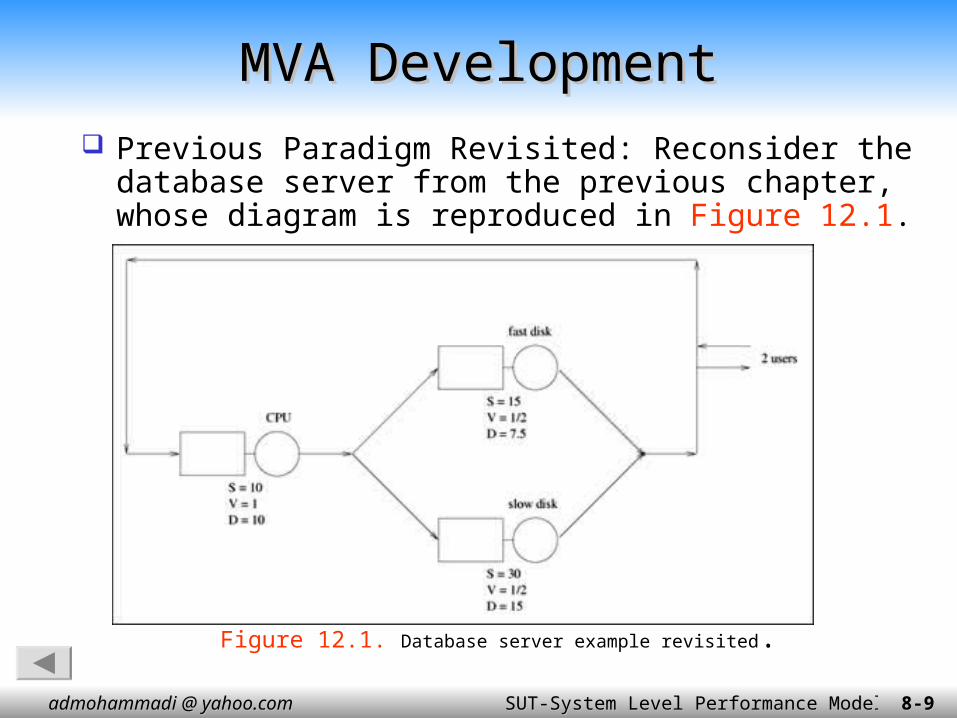
MVA DevelopmentMVA Development Previous Paradigm Revisited: Reconsider the
database server from the previous chapter, whose diagram is reproduced in Figure 12.1.
Figure 12.1. Database server example revisited.

admohammadi @ yahoo.comadmohammadi @ yahoo.com SUT-System Level Performance ModelsSUT-System Level Performance Models8-8-1010
MVA DevelopmentMVA Development S: mean service time per visit, V: average number of visits per transaction D = S x V: total demand per transaction The underlying
Markov model is reproduced in Figure 12.2.

admohammadi @ yahoo.comadmohammadi @ yahoo.com SUT-System Level Performance ModelsSUT-System Level Performance Models8-8-1111
MVA DevelopmentMVA Development
By solving the six balance equations, the steady state probabilities were found to be:
admohammadi @ yahoo.comadmohammadi @ yahoo.com SUT-System Level Performance ModelsSUT-System Level Performance Models8-8-1212
MVA DevelopmentMVA Development
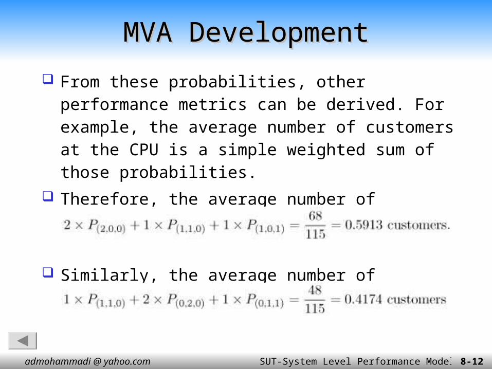
From these probabilities, other performance metrics can be derived. For example, the average number of customers at the CPU is a simple weighted sum of those probabilities.
Therefore, the average number of customers at the CPU is:
Similarly, the average number of customers at the fast disk is:
admohammadi @ yahoo.comadmohammadi @ yahoo.com SUT-System Level Performance ModelsSUT-System Level Performance Models8-8-1313
MVA DevelopmentMVA Development
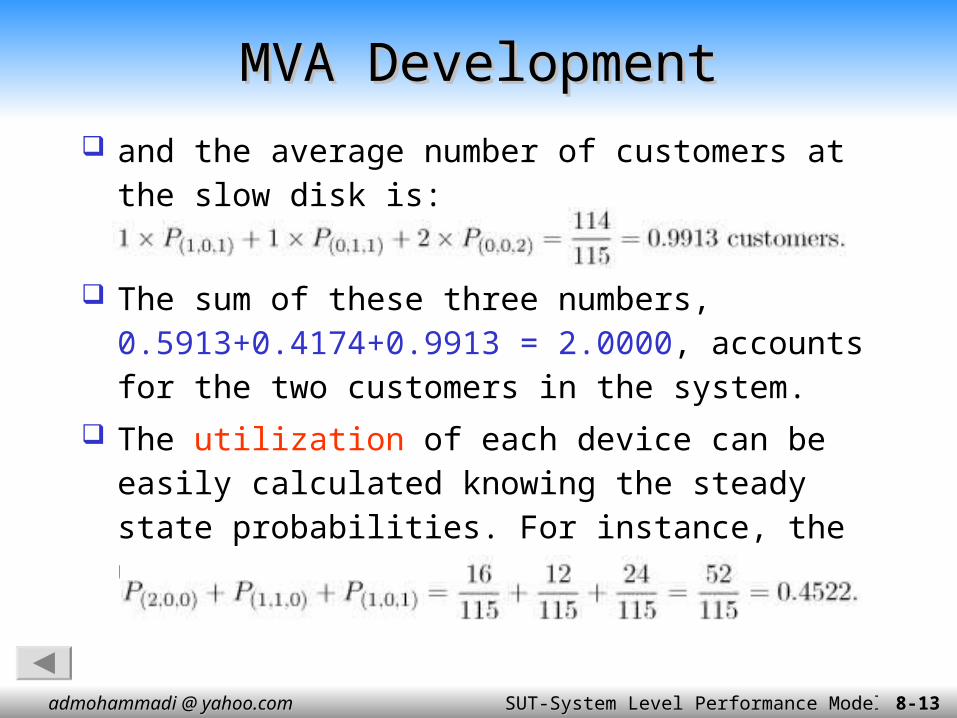
and the average number of customers at the slow disk is:
The sum of these three numbers, 0.5913+0.4174+0.9913 = 2.0000, accounts for the two customers in the system.
The utilization of each device can be easily calculated knowing the steady state probabilities. For instance, the utilization of the CPU is:

admohammadi @ yahoo.comadmohammadi @ yahoo.com SUT-System Level Performance ModelsSUT-System Level Performance Models8-8-1414
MVA DevelopmentMVA Development
Likewise, the utilization of the fast disk is:
and the utilization of the slow disk is:
[Important sidenote: Device utilizations are in the
same ratio as their service demands, regardless
of number of customers in the system (i.e., the
system load).]
admohammadi @ yahoo.comadmohammadi @ yahoo.com SUT-System Level Performance ModelsSUT-System Level Performance Models8-8-1515
MVA DevelopmentMVA Development
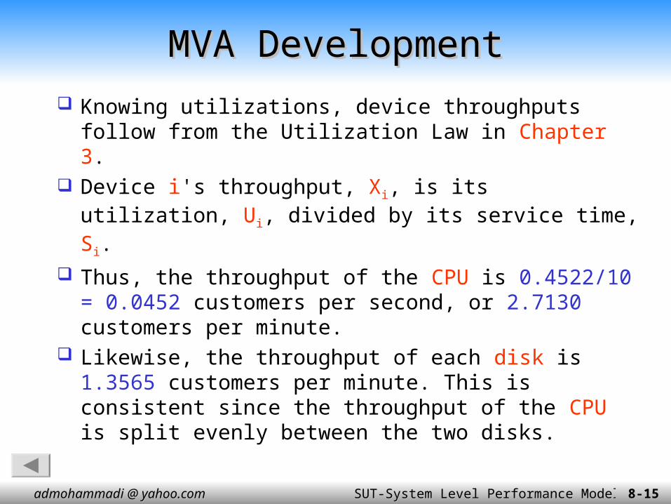
Knowing utilizations, device throughputs follow from the Utilization Law in Chapter 3.
Device i's throughput, Xi, is its utilization, Ui, divided by its service time, Si.
Thus, the throughput of the CPU is 0.4522/10 = 0.0452 customers per second, or 2.7130 customers per minute.
Likewise, the throughput of each disk is 1.3565 customers per minute. This is consistent since the throughput of the CPU is split evenly between the two disks.

admohammadi @ yahoo.comadmohammadi @ yahoo.com SUT-System Level Performance ModelsSUT-System Level Performance Models8-8-1616
MVA DevelopmentMVA Development
Knowing the average number of customers, ni, at
each device and the throughput, Xi, of each
device, the response time, Ri, per visit to each
device is, via Little's Law, the simple ratio of the
two, ni/Xi .
Thus, the response times of the CPU, the fast disk, and the slow disk are 13.08 seconds, 18.46 seconds, and 43.85 seconds, respectively.
admohammadi @ yahoo.comadmohammadi @ yahoo.com SUT-System Level Performance ModelsSUT-System Level Performance Models8-8-1717
MVA DevelopmentMVA Development
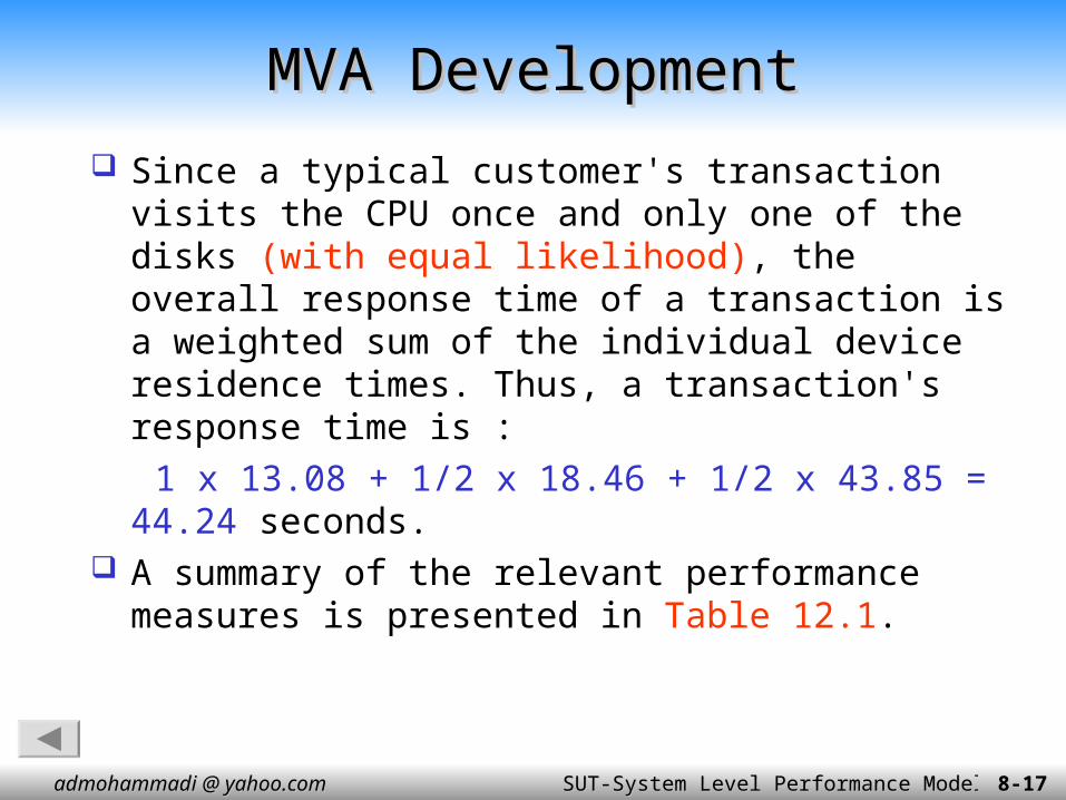
Since a typical customer's transaction visits the CPU once and only one of the disks (with equal likelihood), the overall response time of a transaction is a weighted sum of the individual device residence times. Thus, a transaction's response time is :
1 x 13.08 + 1/2 x 18.46 + 1/2 x 43.85 = 44.24 seconds.
A summary of the relevant performance measures is presented in Table 12.1.

admohammadi @ yahoo.comadmohammadi @ yahoo.com SUT-System Level Performance ModelsSUT-System Level Performance Models8-8-1818
Table 12.1.Table 12.1. Performance Metrics for the Database Server Example (2 customers) Performance Metrics for the Database Server Example (2 customers)
Average Number of Customers
CPUFast diskSlow disk
0.59130.41740.9913
Utilizations (%)
CPUFast diskSlow disk
45.22%33.91%67.83%
Throughputs (customers per minute)
CPUFast diskSlow disk
2.71301.35651.3565
Residence Times (seconds)
CPUFast diskSlow disk
13.089.23
21.93
Response Time (seconds)44.24
admohammadi @ yahoo.comadmohammadi @ yahoo.com SUT-System Level Performance ModelsSUT-System Level Performance Models8-8-1919
MVA DevelopmentMVA Development
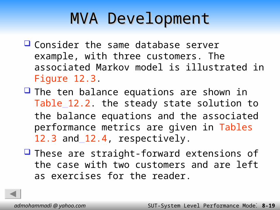
Consider the same database server example, with three customers. The associated Markov model is illustrated in Figure 12.3.
The ten balance equations are shown in Table 12.2. the steady state solution to the balance equations and the associated performance metrics are given in Tables 12.3 and 12.4, respectively.
These are straight-forward extensions of the case with two customers and are left as exercises for the reader.

admohammadi @ yahoo.comadmohammadi @ yahoo.com SUT-System Level Performance ModelsSUT-System Level Performance Models8-8-2020
MVA DevelopmentMVA Development
Figure 12.3. Markov model of the database server example (3
customers).

admohammadi @ yahoo.comadmohammadi @ yahoo.com SUT-System Level Performance ModelsSUT-System Level Performance Models8-8-2121
MVA DevelopmentMVA Development
Table 12.2. Balance Equations for the Database Server Example (3 customers)
admohammadi @ yahoo.comadmohammadi @ yahoo.com SUT-System Level Performance ModelsSUT-System Level Performance Models8-8-2222
MVA DevelopmentMVA Development
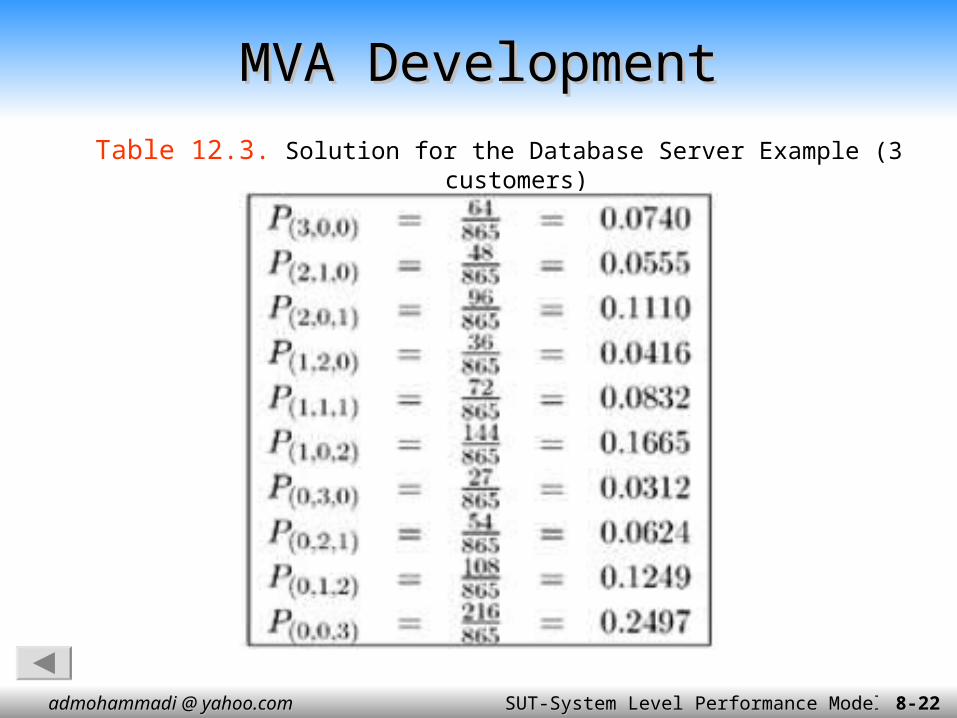
Table 12.3. Solution for the Database Server Example (3 customers)
admohammadi @ yahoo.comadmohammadi @ yahoo.com SUT-System Level Performance ModelsSUT-System Level Performance Models8-8-2323
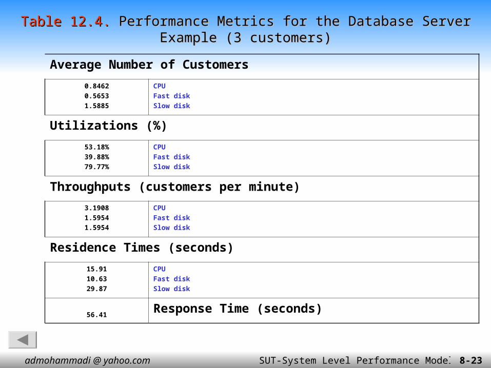
Table 12.4.Table 12.4. Performance Metrics for the Database Server Example (3 customers)Performance Metrics for the Database Server Example (3 customers)
Average Number of Customers
CPUFast diskSlow disk
0.84620.56531.5885
Utilizations (%)
CPUFast diskSlow disk
53.18%39.88%79.77%
Throughputs (customers per minute)
CPUFast diskSlow disk
3.19081.59541.5954
Residence Times (seconds)
CPUFast diskSlow disk
15.9110.6329.87
Response Time (seconds)56.41

admohammadi @ yahoo.comadmohammadi @ yahoo.com SUT-System Level Performance ModelsSUT-System Level Performance Models8-8-2424
MVA DevelopmentMVA Development
[Sidenote: As a consistency check on the performance metrics given in Table 12.4, the sum of the average number of customers at the devices equals the total number of customers in the system (i.e., three). Also, the utilization of the CPU is (2/3) of the slow disk, and the utilization of the slow disk is twice that of the fast disk (i.e.,utilizations remain in the same ratio as their service demands). The throughputs of the disks are identical and sum to that of the CPU.]

admohammadi @ yahoo.comadmohammadi @ yahoo.com SUT-System Level Performance ModelsSUT-System Level Performance Models8-8-2525
The Need for a New Paradigm: The Need for a New Paradigm:
This technique of going from the two customer case to the three customer case does not scale as the number of devices and the number of customers increases.
Arrival Theorem: Given that there are three customers in the network, when a customer arrives at the CPU, the average number of customers that the arriving customer sees already at the CPU is precisely the average number of customers at the CPU with two customers in the network.
admohammadi @ yahoo.comadmohammadi @ yahoo.com SUT-System Level Performance ModelsSUT-System Level Performance Models8-8-2626
Thus, the time it will take for the arriving customer to complete service and leave the CPU (residence time) will be the time it takes to service those customers already at the CPU plus the time it takes to service the arriving customer. Since the average service time per customer at the CPU is 10 seconds, it will take an average of 10 x 0.5913 seconds to service customers already at the CPU, plus 10 seconds to service the arriving customer. Therefore, the residence time is 10(1+0.5913) = 15.91 seconds.
The Need for a New Paradigm:The Need for a New Paradigm:
admohammadi @ yahoo.comadmohammadi @ yahoo.com SUT-System Level Performance ModelsSUT-System Level Performance Models8-8-2727
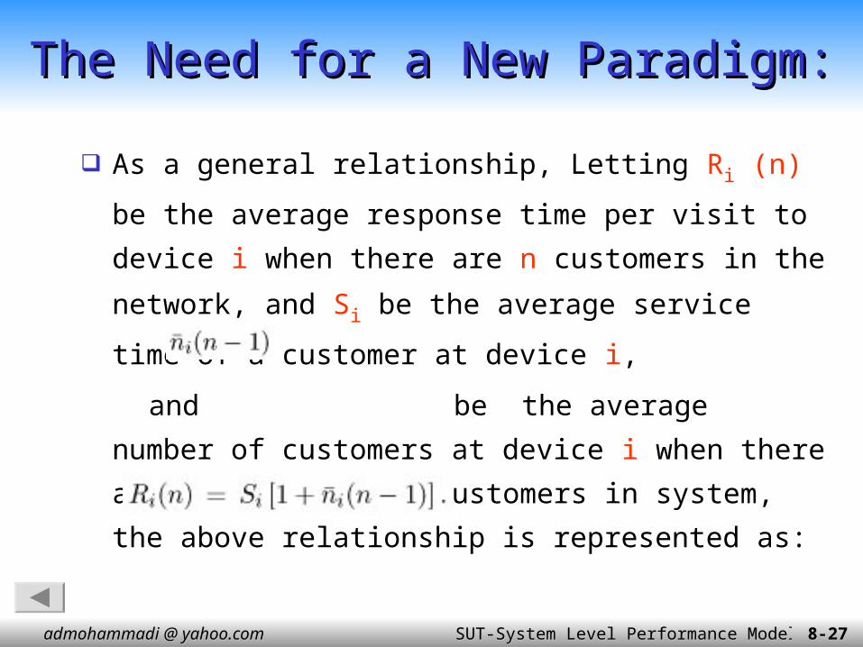
As a general relationship, Letting Ri (n) be the
average response time per visit to device i when
there are n customers in the network, and Si be
the average service time of a customer at device
i,
and be the average number of
customers at device i when there are a total of
n–1 customers in system, the above relationship
is represented as:
The Need for a New Paradigm:The Need for a New Paradigm:

admohammadi @ yahoo.comadmohammadi @ yahoo.com SUT-System Level Performance ModelsSUT-System Level Performance Models8-8-2828
Therefore, the response time at the fast disk, when there are three customers in the network, is the product of its service time (i.e., 15 seconds) and the number of customers at the disk: 15(1 + 0.4174) = 21.36 seconds. Likewise, the residence time at the slow disk is :
30(1 + 0.9913) = 59.74 seconds.
The Need for a New Paradigm:The Need for a New Paradigm:

admohammadi @ yahoo.comadmohammadi @ yahoo.com SUT-System Level Performance ModelsSUT-System Level Performance Models8-8-2929
Now the overall response time, R0(n), is the sum of the residence times .
In database server with three customers, the residence times at CPU, fast disk, and slow disk are 15.91, 21.26,and 59.74 seconds.The number of visits to these devices per transaction is 1.0, 0.5, and 0.5. Thus the overall response time is
(1.0 x 15.91) + (0.5 x 21.26) + (0.5 x 59.74) = 56.41 seconds.
The Need for a New Paradigm:The Need for a New Paradigm:
admohammadi @ yahoo.comadmohammadi @ yahoo.com SUT-System Level Performance ModelsSUT-System Level Performance Models8-8-3030
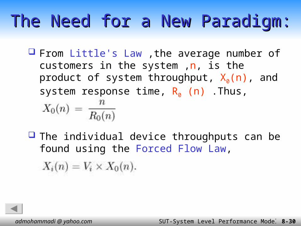
From Little's Law ,the average number of customers in the system ,n, is the product of system throughput, X0(n), and system response time, R0 (n) .Thus,
The individual device throughputs can be found using the Forced Flow Law,
The Need for a New Paradigm:The Need for a New Paradigm:

admohammadi @ yahoo.comadmohammadi @ yahoo.com SUT-System Level Performance ModelsSUT-System Level Performance Models8-8-3131
In the database server with three customers, overall system throughput is
X0 (3) = 3/R(3) = 3/56.41 = 0.0532 customers/second (3.1908 customers/minute).
And the individual device throughputs are 3.1908, 1.5954, and 1.5954 customers per minute.
the device utilizations follow from the device throughputs via the Utilization Law,
The Need for a New Paradigm:The Need for a New Paradigm:
admohammadi @ yahoo.comadmohammadi @ yahoo.com SUT-System Level Performance ModelsSUT-System Level Performance Models8-8-3232
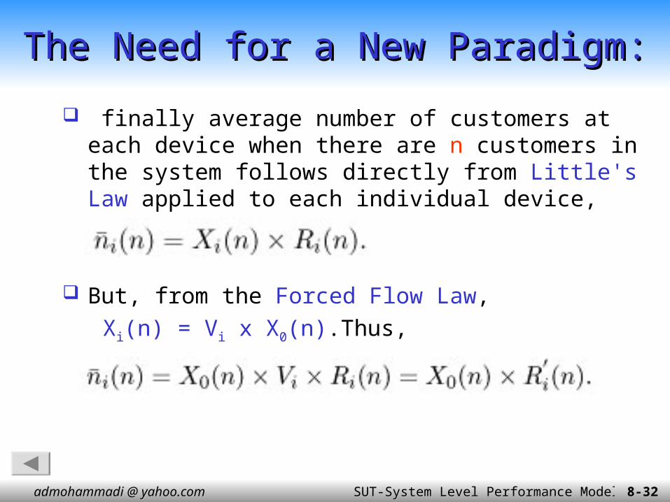
finally average number of customers at each device when there are n customers in the system follows directly from Little's Law applied to each individual device,
But, from the Forced Flow Law, Xi(n) = Vi x X0(n).Thus,
The Need for a New Paradigm:The Need for a New Paradigm:
admohammadi @ yahoo.comadmohammadi @ yahoo.com SUT-System Level Performance ModelsSUT-System Level Performance Models8-8-3333
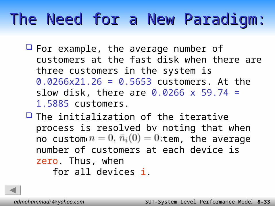
For example, the average number of customers at the fast disk when there are three customers in the system is 0.0266x21.26 = 0.5653 customers. At the slow disk, there are 0.0266 x 59.74 = 1.5885 customers.
The initialization of the iterative process is resolved by noting that when no customers are in system, the average number of customers at each device is zero. Thus, when for all devices i.
The Need for a New Paradigm:The Need for a New Paradigm:
admohammadi @ yahoo.comadmohammadi @ yahoo.com SUT-System Level Performance ModelsSUT-System Level Performance Models8-8-3434
Chapter 12-OutlinesChapter 12-Outlines
12.1 Introduction 12.2 MVA Development 12.3 The MVA Algorithm 12.4 Balanced Systems 12.5 MVA Extensions and Limitations 12.6 Chapter Summary 12.7 Exercises
admohammadi @ yahoo.comadmohammadi @ yahoo.com SUT-System Level Performance ModelsSUT-System Level Performance Models8-8-3535
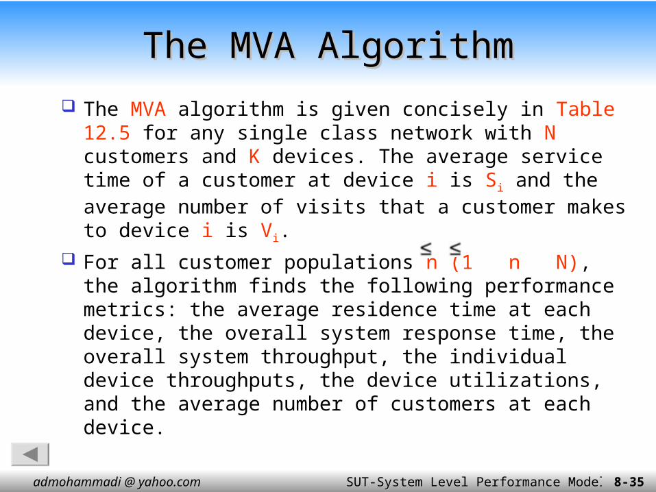
The MVA algorithm is given concisely in Table 12.5 for any single class network with N customers and K devices. The average service time of a customer at device i is Si and the average number of visits that a customer makes to device i is Vi.
For all customer populations n (1 n N), the algorithm finds the following performance metrics: the average residence time at each device, the overall system response time, the overall system throughput, the individual device throughputs, the device utilizations, and the average number of customers at each device.
The MVA AlgorithmThe MVA Algorithm

admohammadi @ yahoo.comadmohammadi @ yahoo.com SUT-System Level Performance ModelsSUT-System Level Performance Models8-8-3636
Initialize the average number of customers at each device i: (0) = 0For each customer population n = 1, 2,... N,calculate the average residence time for each device i:
calculate the overall system response time:
calculate the overall system throughput:
calculate the throughput for each device i:Xi(n) = Vi x X0(n)calculate the utilization for each device i:Ui(n) = Si x Xi(n)calculate the average number of customers at each device i:
Table 12.5.Table 12.5. The MVA Algorithm The MVA Algorithm
admohammadi @ yahoo.comadmohammadi @ yahoo.com SUT-System Level Performance ModelsSUT-System Level Performance Models8-8-3737
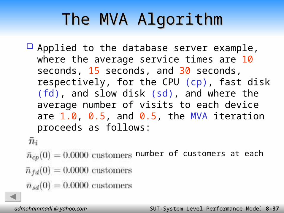
Applied to the database server example, where the average service times are 10 seconds, 15 seconds, and 30 seconds, respectively, for the CPU (cp), fast disk (fd), and slow disk (sd), and where the average number of visits to each device are 1.0, 0.5, and 0.5, the MVA iteration proceeds as follows:
Initialize the average number of customers at each device i:( (0) = 0).
The MVA AlgorithmThe MVA Algorithm

admohammadi @ yahoo.comadmohammadi @ yahoo.com SUT-System Level Performance ModelsSUT-System Level Performance Models8-8-3838
For customer population n = 1, calculate the average residence time for each device i:
Calculate the overall system response time:
Calculate the overall system throughput:
The MVA AlgorithmThe MVA Algorithm

admohammadi @ yahoo.comadmohammadi @ yahoo.com SUT-System Level Performance ModelsSUT-System Level Performance Models8-8-3939
Calculate the throughput for each device i: (Xi(n) = Vi x X0(n)).
Calculate the utilization for each device i: (Ui (n) = Si x Xi (n)).
Calculate the average number of customers at each device i:
( (n) = )
The MVA AlgorithmThe MVA Algorithm

admohammadi @ yahoo.comadmohammadi @ yahoo.com SUT-System Level Performance ModelsSUT-System Level Performance Models8-8-4040
For customer population n = 2, calculate the average residence time for each device i:
Calculate the overall system response time:
The MVA AlgorithmThe MVA Algorithm
admohammadi @ yahoo.comadmohammadi @ yahoo.com SUT-System Level Performance ModelsSUT-System Level Performance Models8-8-4141
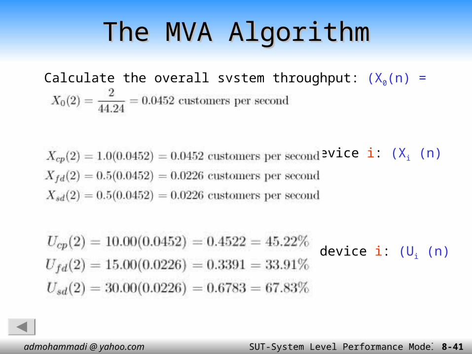
Calculate the overall system throughput: (X0(n) = n/R(n)) .
Calculate the throughput for each device i: (Xi (n) = Vi x X0(n)) .
Calculate the utilization for each device i: (Ui (n) = Si x Xi
(n)) .
The MVA AlgorithmThe MVA Algorithm

admohammadi @ yahoo.comadmohammadi @ yahoo.com SUT-System Level Performance ModelsSUT-System Level Performance Models8-8-4242
Calculate the average number of customers at each device i: ( (n) = X0(n)x ).
For customer population n = 3, calculate the average
residence time for each device i:
The MVA AlgorithmThe MVA Algorithm

admohammadi @ yahoo.comadmohammadi @ yahoo.com SUT-System Level Performance ModelsSUT-System Level Performance Models8-8-4343
Calculate the overall system response time:
Calculate the overall system throughput:
Calculate the throughput for each device i: (Xi (n) = Vi x X0(n)) .
Calculate the utilization for each device i: (Ui (n) = Si x Xi
(n)) .
The MVA AlgorithmThe MVA Algorithm
admohammadi @ yahoo.comadmohammadi @ yahoo.com SUT-System Level Performance ModelsSUT-System Level Performance Models8-8-4444
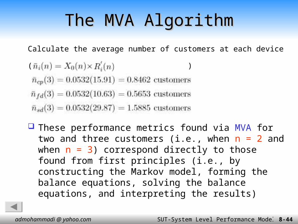
Calculate the average number of customers at each device
( )
These performance metrics found via MVA for two and three customers (i.e., when n = 2 and when n = 3) correspond directly to those found from first principles (i.e., by constructing the Markov model, forming the balance equations, solving the balance equations, and interpreting the results)
The MVA AlgorithmThe MVA Algorithm

admohammadi @ yahoo.comadmohammadi @ yahoo.com SUT-System Level Performance ModelsSUT-System Level Performance Models8-8-4545
Chapter 12-OutlinesChapter 12-Outlines
12.1 Introduction 12.2 MVA Development 12.3 The MVA Algorithm 12.4 Balanced Systems 12.5 MVA Extensions and Limitations 12.6 Chapter Summary 12.7 Exercises

admohammadi @ yahoo.comadmohammadi @ yahoo.com SUT-System Level Performance ModelsSUT-System Level Performance Models8-8-4646
The MVA iteration starts once the customer distribution among the devices is known. That is, knowing how n – 1 customers are distributed among the devices,the performance measures when there are n customers in the system follow directly, as seen from the MVA algorithm given in Table 12.5.
Now consider a balanced system. A system is considered to be balanced if a typical customer places the same average Demand(D) on each of the devices. This implies that all devices are equally utilized.
Balanced SystemsBalanced Systems

admohammadi @ yahoo.comadmohammadi @ yahoo.com SUT-System Level Performance ModelsSUT-System Level Performance Models8-8-4747
A balanced system is not one where all devices are the same speed, only that the faster devices are either visited more often or the demand per visit to them is higher.
A balanced system implies that there is no single bottleneck in the system. Because the bottleneck device would have a greater positive impact on overall performance than improvements made to any other device.
Balanced systems are important to consider, since they provide an upper bound on performance, a gold standard toward which to aspire.
Balanced SystemsBalanced Systems
admohammadi @ yahoo.comadmohammadi @ yahoo.com SUT-System Level Performance ModelsSUT-System Level Performance Models8-8-4848
For example, reconsider the database server example. From Tables 12.1 and 12.4 , the slow disk has the highest utilization and is the bottleneck .So the system is not balanced.
Because the slow disk is over-utilized compared to the other devices, one way to improve performance would be to move some of the files from the slow disk to the fast disk. This has the effect of reducing the load (and utilization) of the slow disk and increasing the load (and utilization) of the fast disk.
Balanced SystemsBalanced Systems
admohammadi @ yahoo.comadmohammadi @ yahoo.com SUT-System Level Performance ModelsSUT-System Level Performance Models8-8-4949
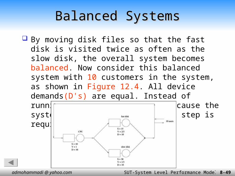
By moving disk files so that the fast disk is visited twice as often as the slow disk, the overall system becomes balanced. Now consider this balanced system with 10 customers in the system, as shown in Figure 12.4. All device demands(D's) are equal. Instead of running 10 iterations of MVA,because the system is balanced,only one MVA step is required;
Balanced SystemsBalanced Systems
admohammadi @ yahoo.comadmohammadi @ yahoo.com SUT-System Level Performance ModelsSUT-System Level Performance Models8-8-5050
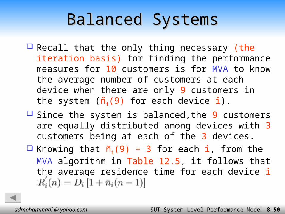
Recall that the only thing necessary (the iteration basis) for finding the performance measures for 10 customers is for MVA to know the average number of customers at each device when there are only 9 customers in the system (ñi(9) for each device i).
Since the system is balanced,the 9 customers are equally distributed among devices with 3 customers being at each of the 3 devices.
Knowing that ñi(9) = 3 for each i, from the MVA algorithm in Table 12.5, it follows that the average residence time for each device i is :
Balanced SystemsBalanced Systems

admohammadi @ yahoo.comadmohammadi @ yahoo.com SUT-System Level Performance ModelsSUT-System Level Performance Models8-8-5151
The overall system response time is:
The overall system throughput is:
Balanced SystemsBalanced Systems

admohammadi @ yahoo.comadmohammadi @ yahoo.com SUT-System Level Performance ModelsSUT-System Level Performance Models8-8-5252
The throughput for each device i (Xi (n) = Vi x X0(n)) is:
The utilization for each device i (Ui (n) = Si x Xi (n))
is:
Balanced SystemsBalanced Systems
admohammadi @ yahoo.comadmohammadi @ yahoo.com SUT-System Level Performance ModelsSUT-System Level Performance Models8-8-5353
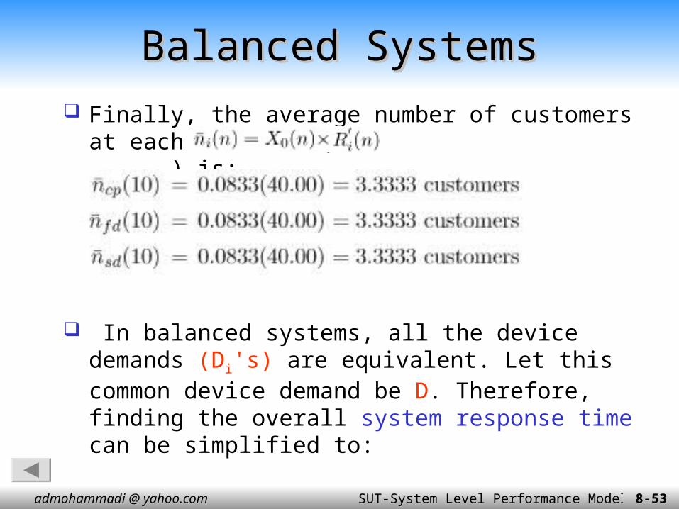
Finally, the average number of customers at each device i ( ) is:
In balanced systems, all the device demands (Di's) are equivalent. Let this common device demand be D. Therefore, finding the overall system response time can be simplified to:
Balanced SystemsBalanced Systems

admohammadi @ yahoo.comadmohammadi @ yahoo.com SUT-System Level Performance ModelsSUT-System Level Performance Models8-8-5454
Balanced SystemsBalanced Systems

admohammadi @ yahoo.comadmohammadi @ yahoo.com SUT-System Level Performance ModelsSUT-System Level Performance Models8-8-5555
and overall system throughput is simply:
As a verification in the balanced database server example, where n = 10, D = 10, and
K = 3, the overall system response time is R0(10) = 10(3 + 10 – 1) = 120 seconds and the overall system throughput is
X0 (10) = 10/120 = 0.0833 customers/second.
Balanced SystemsBalanced Systems
admohammadi @ yahoo.comadmohammadi @ yahoo.com SUT-System Level Performance ModelsSUT-System Level Performance Models8-8-5656
Chapter 12-OutlinesChapter 12-Outlines
12.1 Introduction 12.2 MVA Development 12.3 The MVA Algorithm 12.4 Balanced Systems 12.5 MVA Extensions and Limitations 12.6 Chapter Summary 12.7 Exercises

admohammadi @ yahoo.comadmohammadi @ yahoo.com SUT-System Level Performance ModelsSUT-System Level Performance Models8-8-5757
MVA algorithm has been the focus of much researchs. These include:
1. Multi-class networks2. Networks with load dependent servers3. Networks with open and closed classes of
customers The extension of MVA to product form, load-
independent, multi-class networks is the topic of Chapter 13 . Chapter 14 extends MVA and the treatment of multiclass open QNs to the load-dependent case. Approximations to deal with non-product form QNs are presented in Chapter 15.
MVA Extensions and LimitationsMVA Extensions and Limitations

admohammadi @ yahoo.comadmohammadi @ yahoo.com SUT-System Level Performance ModelsSUT-System Level Performance Models8-8-5858
1. MVA does not provide the steady state probabilities of individual system states.
2. MVA does not provide transient analysis information.
3. MVA does not model state dependent behavior.
4. MVA solves product form networks. As a result, MVA is not directly applicable to non-product form situations.
limitations and shortcomings surrounding limitations and shortcomings surrounding MVA MVA

admohammadi @ yahoo.comadmohammadi @ yahoo.com SUT-System Level Performance ModelsSUT-System Level Performance Models8-8-5959
Chapter 12-OutlinesChapter 12-Outlines
12.1 Introduction 12.2 MVA Development 12.3 The MVA Algorithm 12.4 Balanced Systems 12.5 MVA Extensions and Limitations 12.6 Chapter Summary 12.7 Exercises
admohammadi @ yahoo.comadmohammadi @ yahoo.com SUT-System Level Performance ModelsSUT-System Level Performance Models8-8-6060
The Mean Value Analysis technique is arguably one of the most significant contributions to the field of performance evaluation within the past 25 years. It is the primary solution engine behind the large majority of state-of-the-art analytical solution packages currently in use. MVA is intuitive, elegant, and simple.
This chapter first motivates, then develops, then summarizes, then applies, and finally qualifies MVA. Examples from the database server example introduced in previous chapters are used to demonstrate MVA. The following exercises are intended to reinforce and to broaden the reader's understanding and range of applicability of MVA.
Chapter SummaryChapter Summary

admohammadi @ yahoo.comadmohammadi @ yahoo.com SUT-System Level Performance ModelsSUT-System Level Performance Models8-8-6161


