AdS/CFT Correspondencewith Applications to Condensed Matter

Robert Graham

SFB/TR 12: Symmetries and Universality in Mesoscopic Systems

1

I. Quantum Field Theory and Gauge Theory

II. Conformal Field Theory

III. Short Introduction to Supersymmetry

IV. General Relativity

V. Some String Theory Introduction

VI. A hand-waving derivation of AdS/CFT

VII. Holographic superconductors

2

Holographic superconductors

G. Horowitz 2010 [hep-th 1002.1722]with figures taken from G. Horowitz, Holographic superconductors, MilosLectures 1-2, 2010.

1. Superconductivity

• resistivity drops to 0 below Tc• magnetic field is expelled below Tc, Meissner effect,

perfect diamagnetism

3

London 1935:

J = −λA ⇒ ∂J

∂t∼ −∂A

∂t∼ E

E-field accelerates charge

rotB = 4πJ = −4πλA ⇒∇2 B = 4πλ B

B-field has finite penetration-depth

Landau, Ginzburg 1950, order parameter complex field φ

F = α(T − Tc) |φ|2 +β

2|φ|4 + ξ2 |∇φ|2 ; α, β > 0

T > Tc φ = 0 , T < Tc |φ|2 = α

β|T − Tc|

microscopic theory BCS 1957:electrons interact via phonons and can form pairs of opposite spin,charged bosons which condense below Tc ;

4

pairs are loosely bound, and much larger than lattice spacing.

Ground state: energy gap for creation of charged excitation= dressed electrons and holes

energy gap ∆ ≃ 1.7 Tc .

Optical conductivity σ(ω) has a gap

ωg = 2∆ ≃ 3.5 Tc .

Highest Tc of a BCS-superconductor is about 40◦K (Mg B2 2001)

High Tc (Bednorz and Muller) 1986cuprate compounds with CuO2 planes;highest Tc for a Hg-Ba-CuO2 compound

Tc = 134◦K at normal pressure

∼ 160◦K at higher pressure5

In 2008 Fe instead of Cu,

also in a layered structure

(iron pnictides, with other elements of nitrogen group, like As.)

Again electron pairs, but with unknown pairing mechanism.

The pairing mechanism must come from strong coupling.

AdS/CFT seems to be a good tool to study it.

So far only in models. No connection yet with a microscopic theory.

In his review Horowitz remarks:

6

2. Gravitational dual model

Want to have an AdS background to describe a strongly coupled fieldtheory by a weakly coupled gravitational field in AdS.

Need a black hole in that background with surface gravity κ, to intro-duce a finite temperature T = κ/2π.

The black hole should be planar and parallel to the boundary of AdS(translational invariance).

Black holes in AdS: their Hawking temperature increases with theirmass⇒ positive specific heat.

Need a “black hole with hair”,namely with a condensate at small T , which breaks a global U(1).

7

Idea of S. Gubser, PR D, 78 (2008):

S =

∫

dD+1x

√−g(

R+6

L2︸︷︷︸ւ

−14Fµν F

µν

︸ ︷︷ ︸ց

−|∇ψ − iqAψ|2−m2|ψ|2︸ ︷︷ ︸

↓

)

for AdS with black hole, U(I)-gauge theory scalar ’hair’cosm. constant in bulk with mass m, charge q

∧ = − 3

L2

herem2

eff = m2 + q2 gtt︸︷︷︸<0

A2t

may become negative near horizon where gtt → −0⇒ ψ = 0 becomes unstable.

The instability happens as T is lowered, because as T → 0

the charged Reissner-Nordstrøm b.h. gets closer to extremality(M → Q+) , but then gtt → 0 with double root at horizon, and hencegtt → −∞ even faster.

8

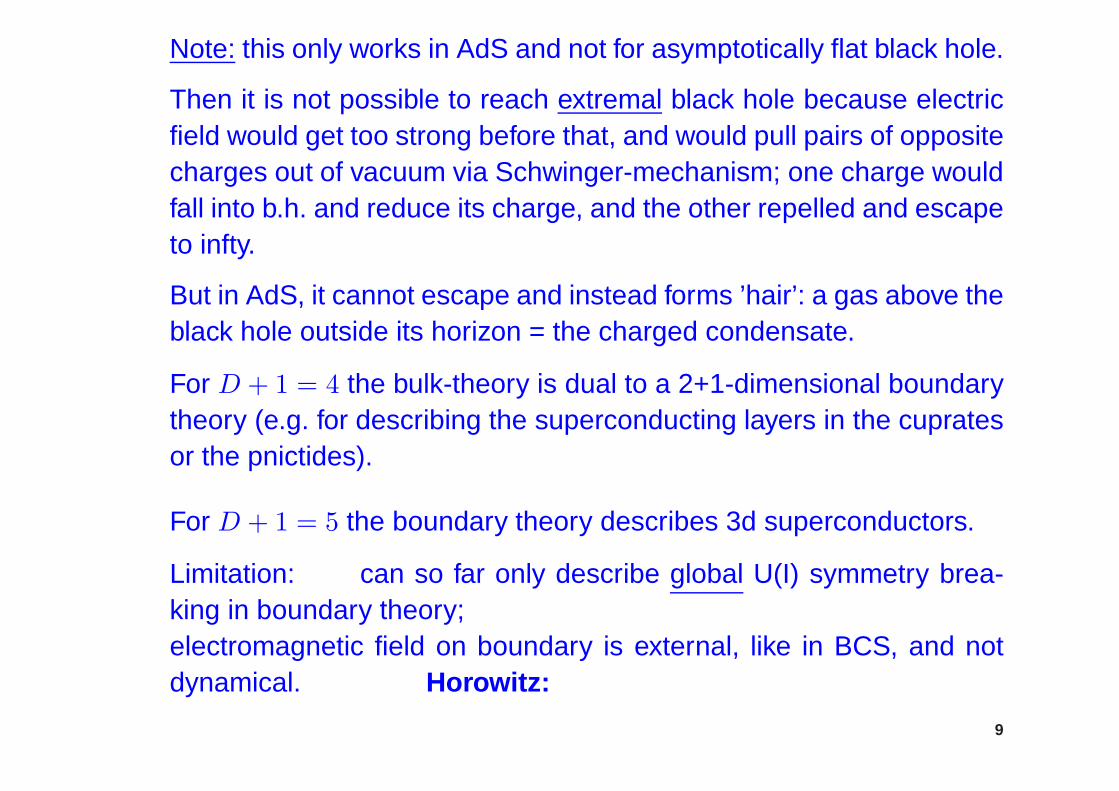
Note: this only works in AdS and not for asymptotically flat black hole.

Then it is not possible to reach extremal black hole because electricfield would get too strong before that, and would pull pairs of oppositecharges out of vacuum via Schwinger-mechanism; one charge wouldfall into b.h. and reduce its charge, and the other repelled and escapeto infty.

But in AdS, it cannot escape and instead forms ’hair’: a gas above theblack hole outside its horizon = the charged condensate.

For D + 1 = 4 the bulk-theory is dual to a 2+1-dimensional boundarytheory (e.g. for describing the superconducting layers in the cupratesor the pnictides).

For D + 1 = 5 the boundary theory describes 3d superconductors.

Limitation: can so far only describe global U(I) symmetry brea-king in boundary theory;electromagnetic field on boundary is external, like in BCS, and notdynamical. Horowitz:

9

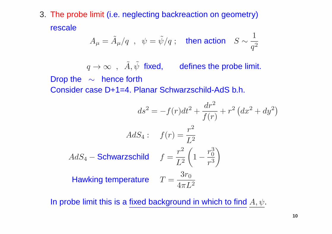
3. The probe limit (i.e. neglecting backreaction on geometry)

rescale

Aµ = Aµ/q , ψ = ψ/q ; then action S ∼ 1

q2

q →∞ , A, ψ fixed, defines the probe limit.

Drop the ∼ hence forthConsider case D+1=4. Planar Schwarzschild-AdS b.h.

ds2 = −f(r)dt2 + dr2

f(r)+ r2

(dx2 + dy2

)

AdS4 : f(r) =r2

L2

AdS4 − Schwarzschild f =r2

L2

(

1− r30

r3

)

Hawking temperature T =3r04πL2

In probe limit this is a fixed background in which to find A,ψ.

10

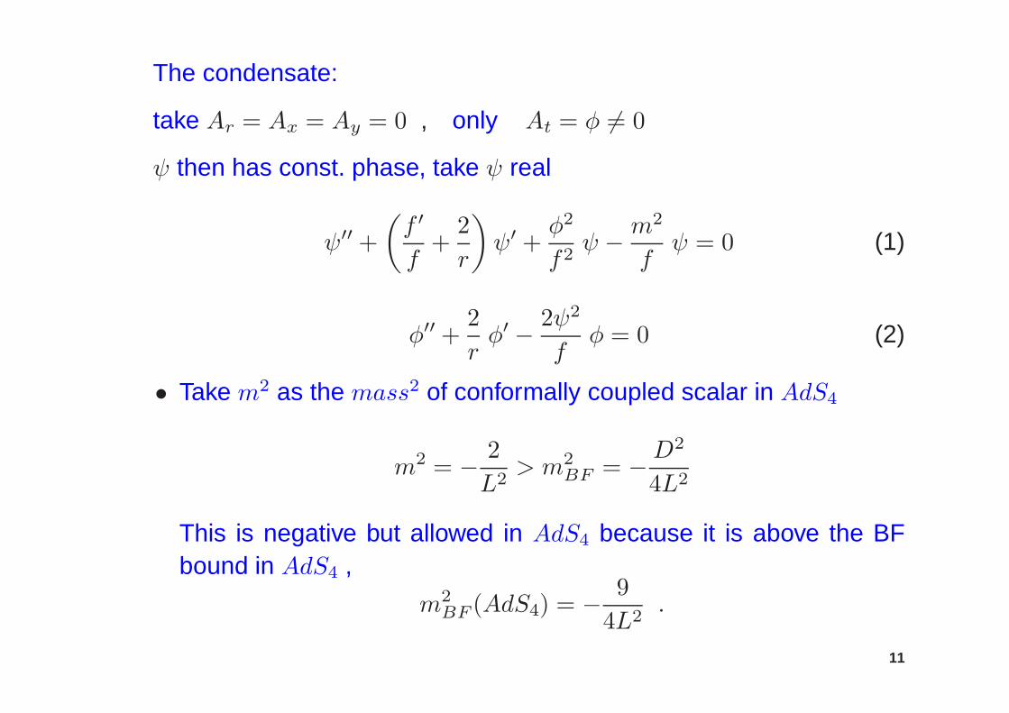
The condensate:

take Ar = Ax = Ay = 0 , only At = φ 6= 0

ψ then has const. phase, take ψ real

ψ′′ +

(f ′

f+

2

r

)

ψ′ +φ2

f2ψ − m

2

fψ = 0 (1)

φ′′ +2

rφ′ − 2ψ2

fφ = 0 (2)

• Take m2 as the mass2 of conformally coupled scalar in AdS4

m2 = − 2

L2> m2

BF = −D2

4L2

This is negative but allowed in AdS4 because it is above the BFbound in AdS4 ,

m2BF (AdS4) = −

9

4L2.

11

• Boundary condition at r = r0 :

A0 = 0 for gµνAµAν to remain finite;

(or gµνAν ∼ jµ to stay finite,

or from eq. (2) at r = r0 , where f(r0) = 0 )

f ′ψ′ = m2ψ (from eq. (1) at r = r0 )

Boundary condition at r →∞ (boundary of AdS4 )

asymptotics of solution

ψ =ψ(1)

r+ψ(2)

r2+ . . .

φ = µ− ρ

r2

’standard‘ b.c.: ψ(1) = 0 , ψ(2) 6= 0 , ψ ∼ 1r2

near boundary’nonstandard‘ b.c.: ψ(2) = 0 , ψ(1) 6= 0 , ψ ∼ 1

r is also possible.

Numerical solution in Hartnoll, Herzog, Horowitz, PRL 101 (2008).

12

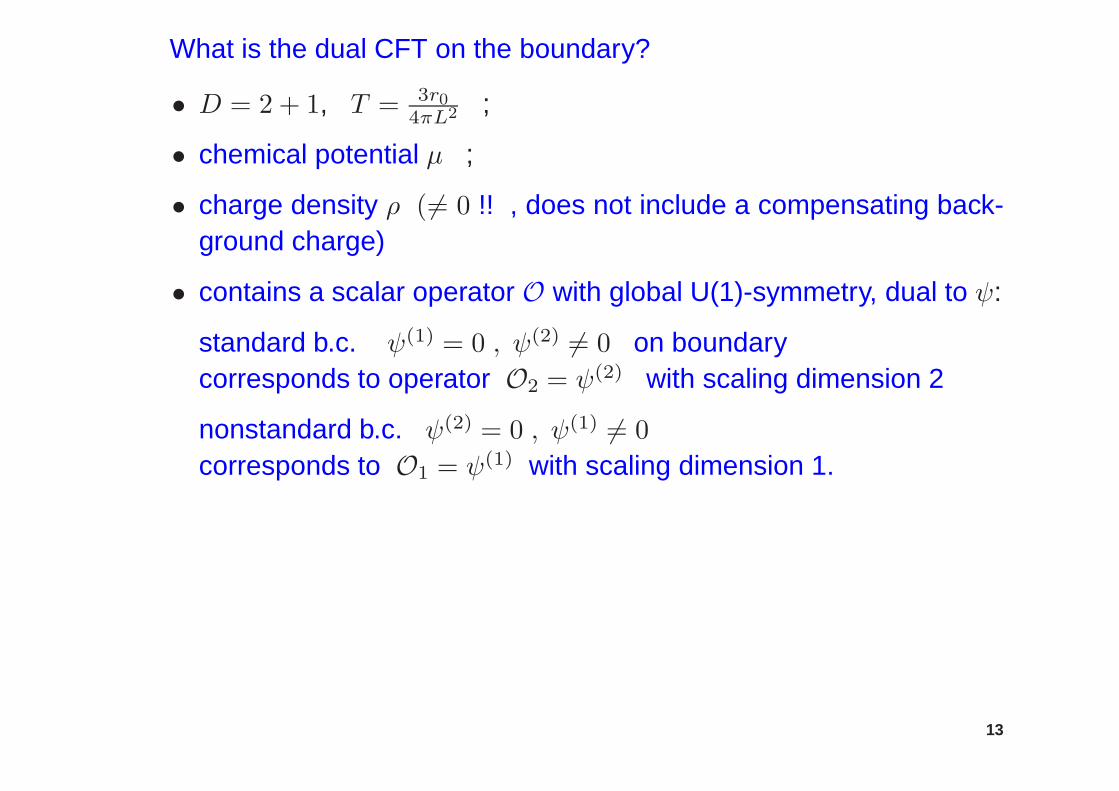
What is the dual CFT on the boundary?

• D = 2 + 1, T = 3r04πL2 ;

• chemical potential µ ;

• charge density ρ ( 6= 0 !! , does not include a compensating back-ground charge)

• contains a scalar operator O with global U(1)-symmetry, dual to ψ:

standard b.c. ψ(1) = 0 , ψ(2) 6= 0 on boundarycorresponds to operator O2 = ψ(2) with scaling dimension 2

nonstandard b.c. ψ(2) = 0 , ψ(1) 6= 0

corresponds to O1 = ψ(1) with scaling dimension 1.

13

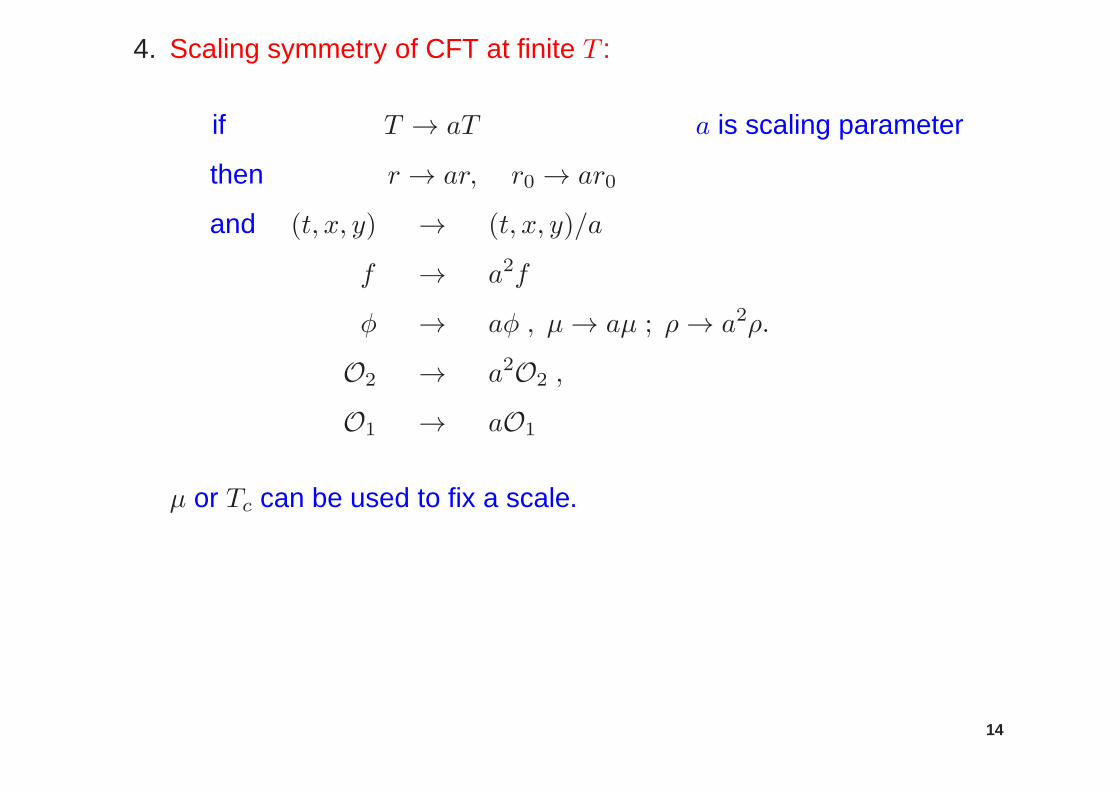
4. Scaling symmetry of CFT at finite T :

if T → aT a is scaling parameter

then r → ar, r0 → ar0

and (t, x, y) → (t, x, y)/a

f → a2f

φ → aφ , µ→ aµ ; ρ→ a2ρ.

O2 → a2O2 ,

O1 → aO1

µ or Tc can be used to fix a scale.

14

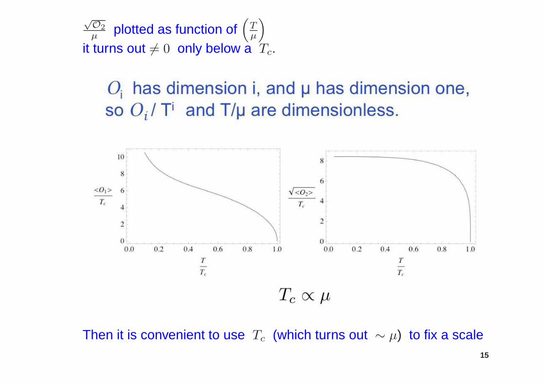
√O2µ plotted as function of

(Tµ

)

it turns out 6= 0 only below a Tc.

Then it is convenient to use Tc (which turns out ∼ µ) to fix a scale15

Behavior near Tc from numerical result

< O1 > ≃ 9.3 Tc (1− T/Tc)1/2

< O2 > ≃ (12 Tc)2 (1− T/Tc)1/2

Free energy (= Euclidean action). Is smaller than Euclidean action

at ψ = 0 , φ = µ− ρr

and becomes equal for T → Tc

=⇒ second order phase transistion.

16

5. Arbitrary mass for field ψ

In AdSD+1 with z = −L2

r

ds2 = L2 dz2 + dxµdxµ

z2= gAB dxA dxB

A = 0 . . .D , xA = (z, xµ) ,√

|g| = L2

z2

S = −κ2

∫

dD+1x√

|g|[gAB∂A ψ ∂B ψ +m2ψ2 +O(ψ3)

]

by partial integration with respect to z from horizon z = −∞ to boun-dary z = −ǫ and using Stokes’ theorem

= −κ2

∫

∂(AdS)

dDx√

|g| gzB ψ ∂Bψ −κ

2

∫

dD+1x√

|g| ψ(

−✷+m2 +O(ψ2))

ψ︸ ︷︷ ︸

=0 on shell

only the boundary term remains.

17

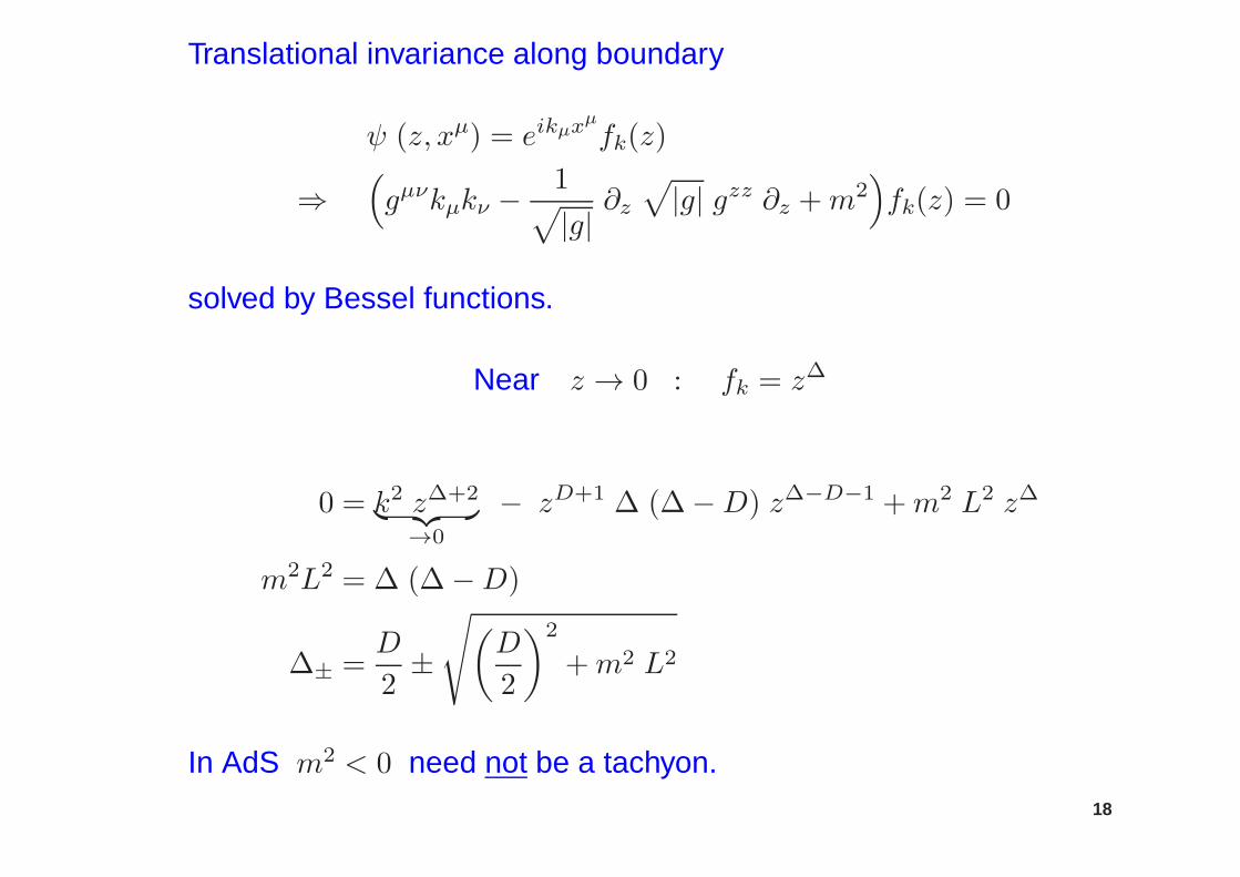
Translational invariance along boundary

ψ (z, xµ) = eikµxµfk(z)

⇒(

gµνkµkν −1√

|g|∂z√

|g| gzz ∂z +m2)

fk(z) = 0

solved by Bessel functions.

Near z → 0 : fk = z∆

0 = k2 z∆+2︸ ︷︷ ︸

→0

− zD+1 ∆ (∆−D) z∆−D−1 +m2 L2 z∆

m2L2 = ∆ (∆−D)

∆± =D

2±

√(D

2

)2

+m2 L2

In AdS m2 < 0 need not be a tachyon.18

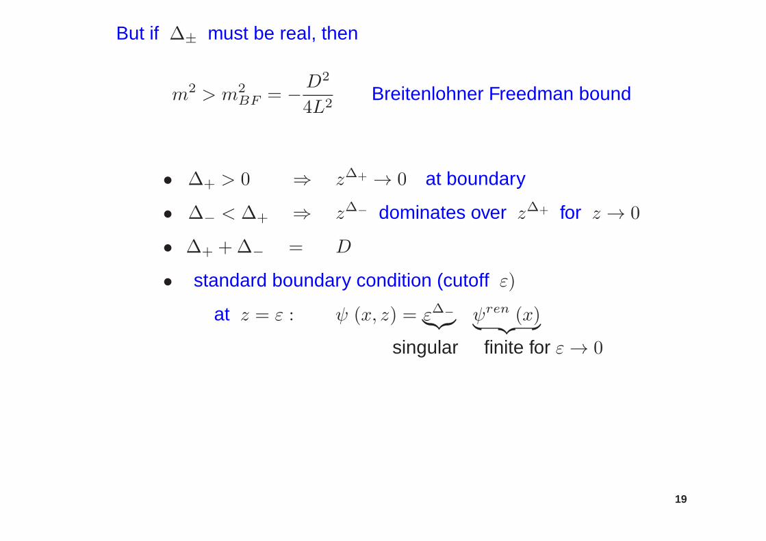
But if ∆± must be real, then

m2 > m2BF = −D

2

4L2Breitenlohner Freedman bound

• ∆+ > 0 ⇒ z∆+ → 0 at boundary

• ∆− < ∆+ ⇒ z∆− dominates over z∆+ for z → 0

• ∆+ +∆− = D

• standard boundary condition (cutoff ε)

at z = ε : ψ (x, z) = ε∆−︸︷︷︸ ψren (x)

︸ ︷︷ ︸

singular finite for ε→ 0

19

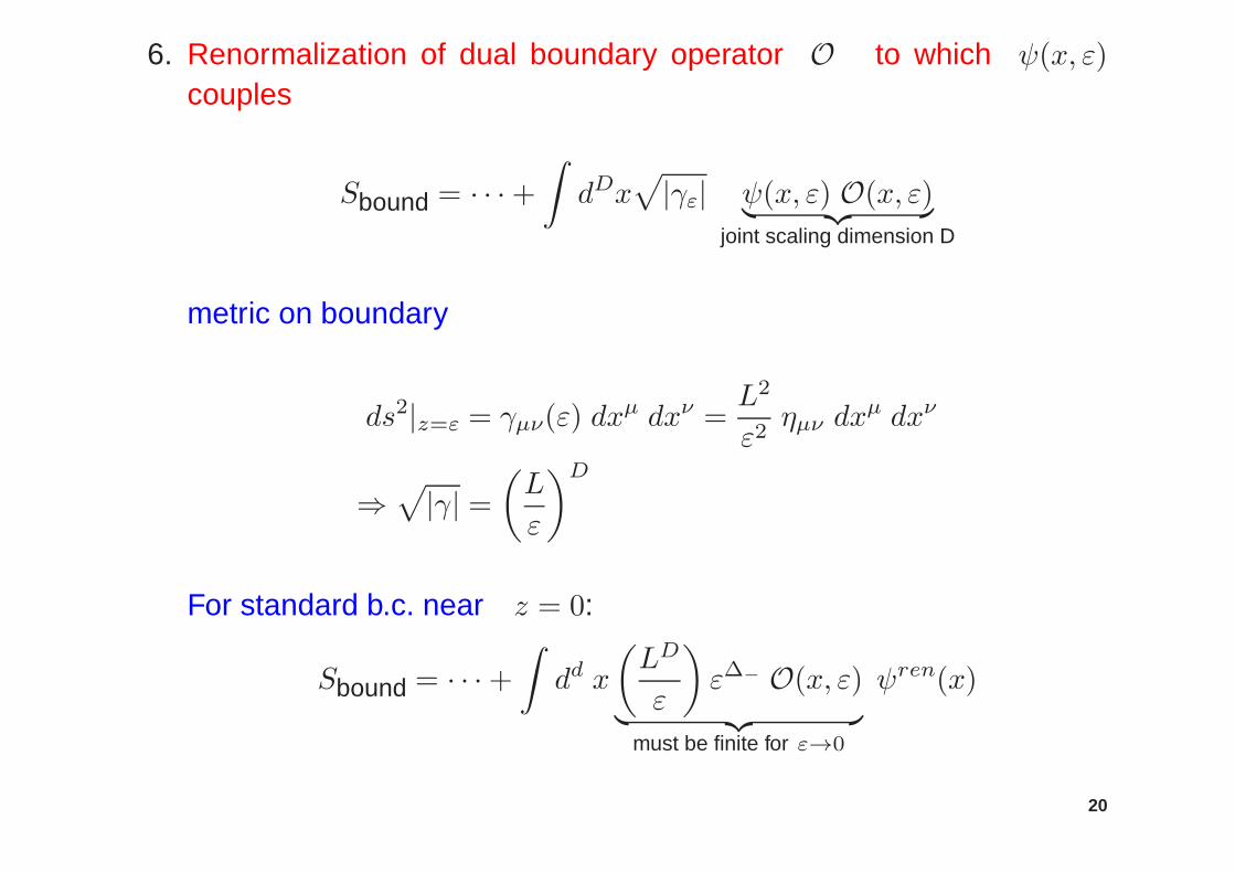
6. Renormalization of dual boundary operator O to which ψ(x, ε)

couples

Sbound = · · ·+∫

dDx√

|γε| ψ(x, ε) O(x, ε)︸ ︷︷ ︸

joint scaling dimension D

metric on boundary

ds2|z=ε = γµν(ε) dxµ dxν =

L2

ε2ηµν dx

µ dxν

⇒√

|γ| =(L

ε

)D

For standard b.c. near z = 0:

Sbound = · · ·+∫

dd x

(LD

ε

)

ε∆− O(x, ε)︸ ︷︷ ︸

must be finite for ε→0

ψren(x)

20

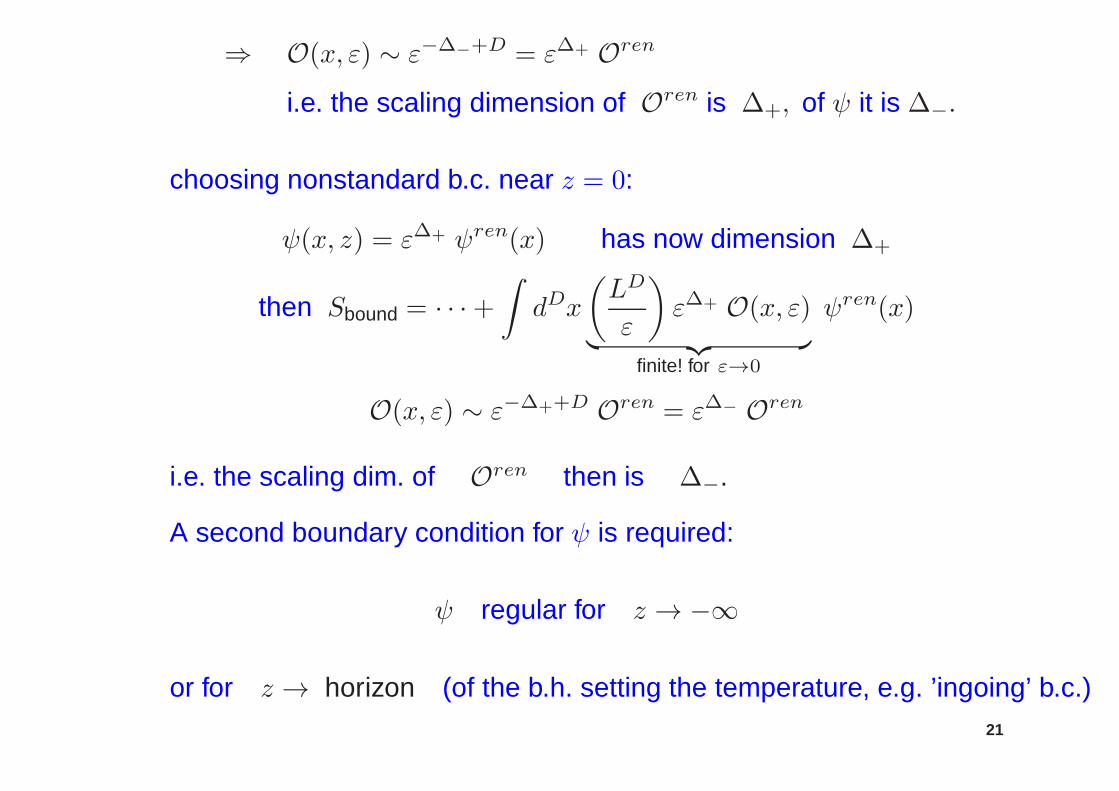
⇒ O(x, ε) ∼ ε−∆−+D = ε∆+ Oren

i.e. the scaling dimension of Oren is ∆+, of ψ it is ∆−.

choosing nonstandard b.c. near z = 0:

ψ(x, z) = ε∆+ ψren(x) has now dimension ∆+

then Sbound = · · ·+∫

dDx

(LD

ε

)

ε∆+ O(x, ε)︸ ︷︷ ︸

finite! for ε→0

ψren(x)

O(x, ε) ∼ ε−∆++D Oren = ε∆− Oren

i.e. the scaling dim. of Oren then is ∆−.

A second boundary condition for ψ is required:

ψ regular for z → −∞

or for z → horizon (of the b.h. setting the temperature, e.g. ’ingoing’ b.c.)21

Note:

• ∆± independent of k and x (typical for a local QFT)

• if m2 > 0 ∆+ > D , O then ”irrelevant“irrelevant means getting weak towards infrared, growing strong to-wards ultraviolet

• if m2 < 0 , then ∆+ < D , O then ”relevant“i.e. growing strong in infrared, growing weak in ultraviolet;ψ ∼ z∆± then both decay towards boundary

• if m2 = 0←→ ∆+ = D , ∆− = 0 , O then ”marginal“

Applied to AdS4, with mass m for scalar ψ:

for r →∞ : ψ =ψ−r∆−

+ψ+

r∆+

∆± =1

2

(

3±√

9 + 4(mL)2)

22

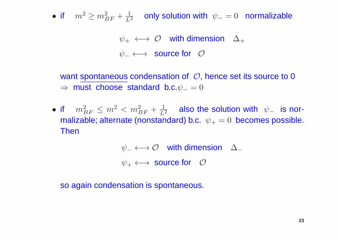
• if m2 ≥ m2BF + 1

L2 only solution with ψ− = 0 normalizable

ψ+ ←→ O with dimension ∆+

ψ−←→ source for O

want spontaneous condensation of O, hence set its source to 0⇒ must choose standard b.c.ψ− = 0

• if m2BF ≤ m2 < m2

BF + 1L2 also the solution with ψ− is nor-

malizable; alternate (nonstandard) b.c. ψ+ = 0 becomes possible.Then

ψ−←→ O with dimension ∆−

ψ+←→ source for O

so again condensation is spontaneous.

23

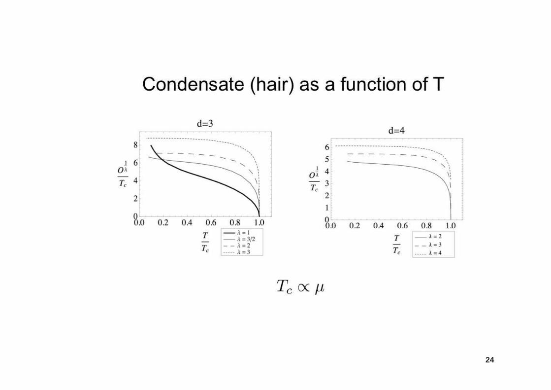
24

here λ is the same as ∆ in our notation

note:the curves λ = 1 , λ = 2 both correspond to (mL)2 = −2, butdifferent b.c.:

λ = 1 : alternateλ = 2 : standard

all other curves are for standard b.c..The curve

• λ = 3 corresponds to m2 = 0

• λ =3

2to m2 = m2

BF = − 9

4L2

25

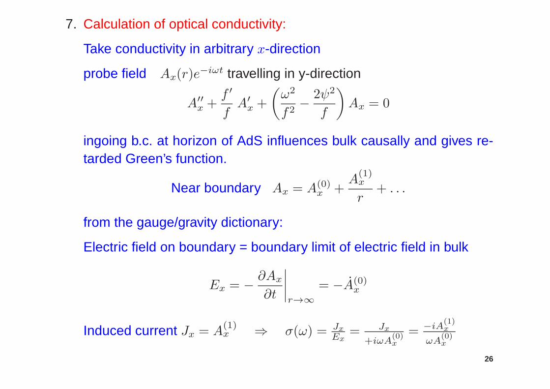
7. Calculation of optical conductivity:

Take conductivity in arbitrary x-direction

probe field Ax(r)e−iωt travelling in y-direction

A′′x +

f ′

fA′

x +

(ω2

f2− 2ψ2

f

)

Ax = 0

ingoing b.c. at horizon of AdS influences bulk causally and gives re-tarded Green’s function.

Near boundary Ax = A(0)x +

A(1)x

r+ . . .

from the gauge/gravity dictionary:

Electric field on boundary = boundary limit of electric field in bulk

Ex = − ∂Ax

∂t

∣∣∣∣r→∞

= −A(0)x

Induced current Jx = A(1)x ⇒ σ(ω) = Jx

Ex= Jx

+iωA(0)x

= −iA(1)x

ωA(0)x

26

Re σ( ωTc) for successively lower temperatures

27

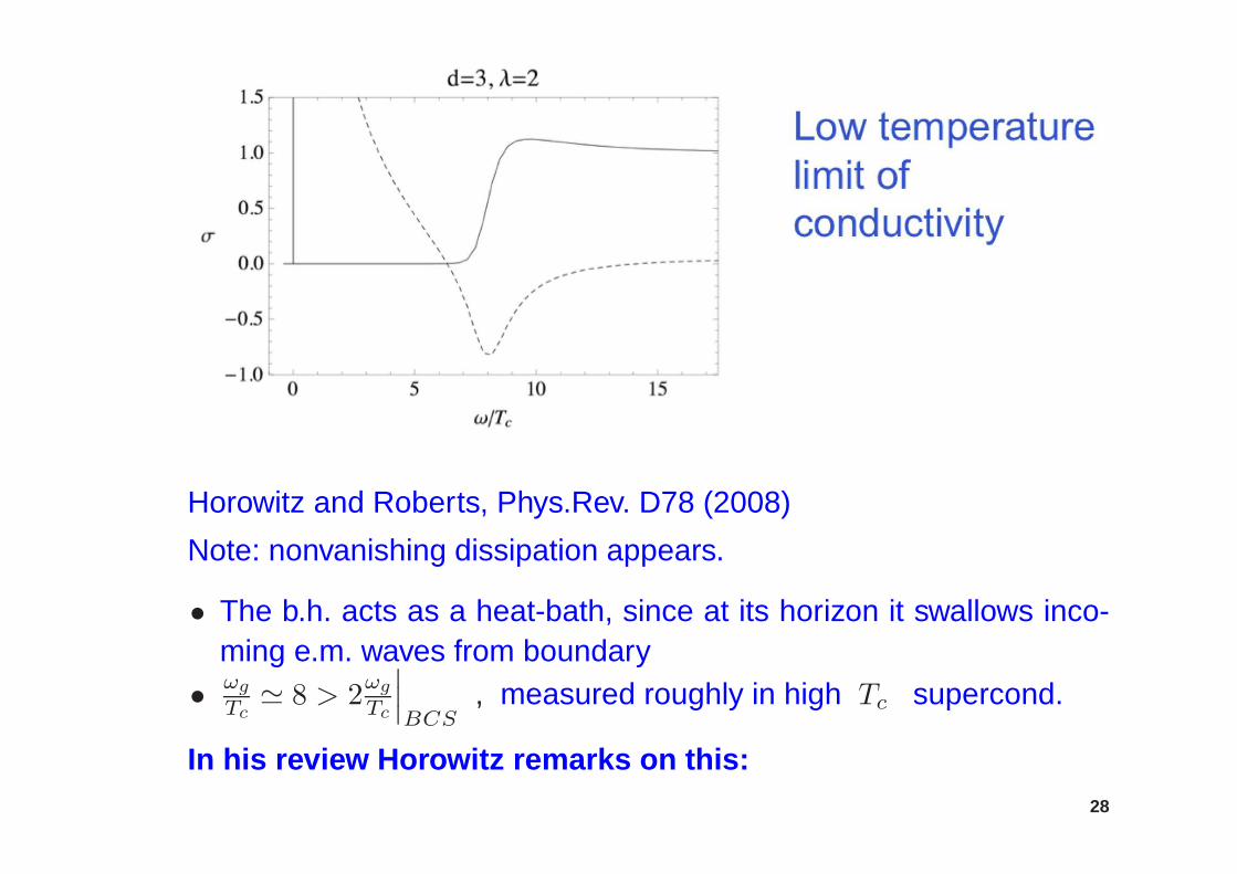
Horowitz and Roberts, Phys.Rev. D78 (2008)

Note: nonvanishing dissipation appears.

• The b.h. acts as a heat-bath, since at its horizon it swallows inco-ming e.m. waves from boundary• ωg

Tc≃ 8 > 2

ωg

Tc

∣∣∣BCS

, measured roughly in high Tc supercond.

In his review Horowitz remarks on this:28

For T < Tc:Im σ(ω) has a pole at ω = 0,(

follows already from⇀j= ne

⇀v= σ

⇀

E

Drude model mdv

dt= eE −mv

τ,

i.e. σ(ω) =ne2

m

τ

1− iωτ ;

τ →∞ : Im σ =ne2

mω, Re σ =

πne2

mδ(ω)

is implied by Kramers-Kronig relation

Im σ(ω) = P+∞∫

−∞

dω′

π

Re σ(ω′)

ω − ω′

)

Re σ(ω′) must therefore contain δ(ω′)

29

8. London equation:

choose Coulomb gauge in boundary,⇀

∇ ·A = 0

Solve equations for Ax(r) and ψ for a wave travelling iny-direction with r-dependent amplitude

Ax = Ax(r)e−iωt+iky

(fA′x)

′+

(

ω2

f2− k2

r2︸︷︷︸only change

)

Ax = 2ψ2Ax

asymptotic for r →∞

Ax(ω, k) = A(0)x (ω, k) +

A(1)x (ω, k)

r+ . . .

⇀

k ·A(0) = 0 =⇀

k ·A(1) (Coulomb-gauge)30

retarded Green’s function for Jx = A(1)x in dual field theory

GR(ω, k) =A

(1)x (ω, k)

A(0)x (ω, k)

= iωσ(ω, k)

In boundary

Jx(ω, k) = A(1)x (ω, k) , Ex = iωA(0)

x (ω, k)

our earlier calculation showed that Im σ(ω) has a pole at ω = 0:

Im σ(ω) =nsω

+ regular ;

Kramers-Kronig relation then implies:

Re σ(ω) = +π nsδ(ω) + regular

⇒ for ω, k → 0 A(1)x︸︷︷︸l

(ω, k) = −nsA(0)x︸︷︷︸l

(ω, k)

i.e. in boundary Jx (ω, k) = −ns Ax(ω, k) London eqn.31

Further results for holographic superconductor(Herzog at al., Horowitz et al.)

From retarded Green’s function

GR(ω, k) =A(1)(ω, k)

A(0)(ω, k)

by expansion in k2 :

Im GR(ω, k) = −ns (1 + ξ2k k2 + . . . )

Near Tc

ξ Tc ≃0.1

(1− T/Tc)1/2

32

33

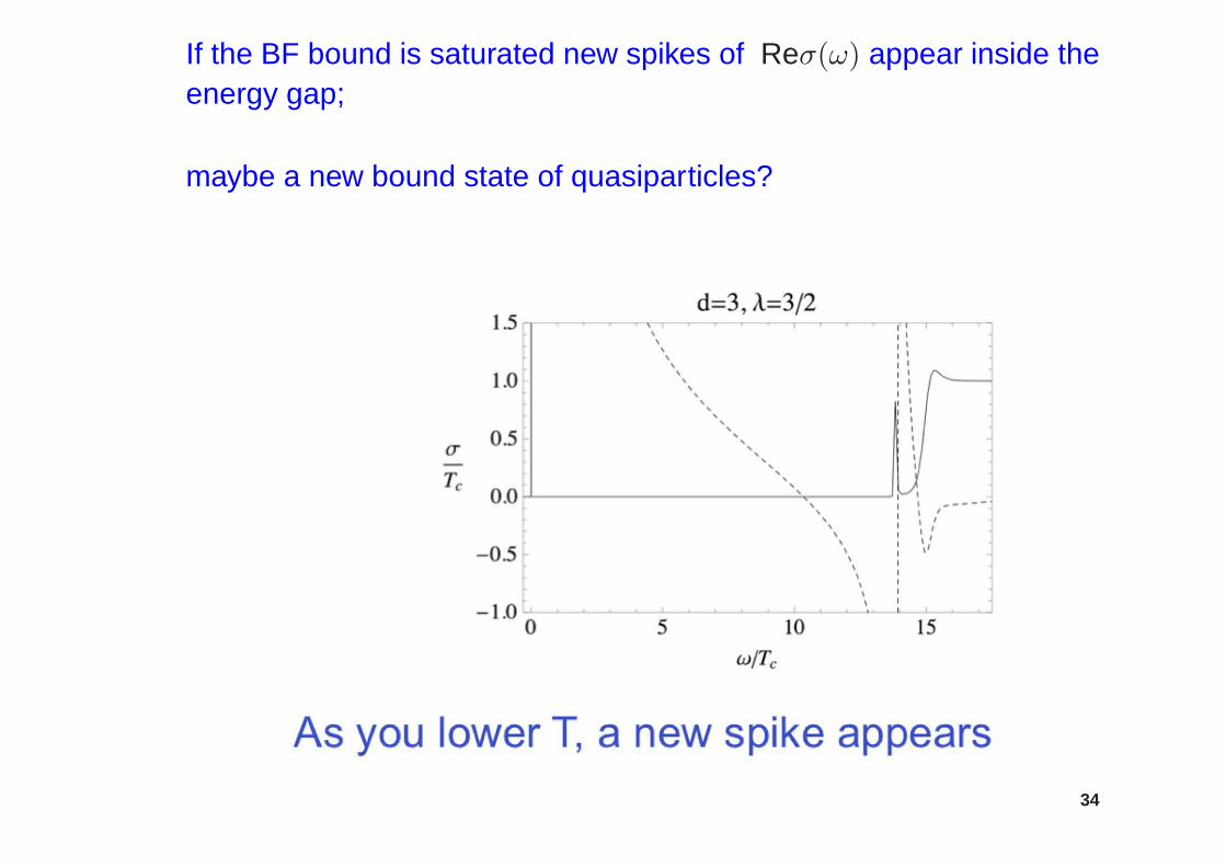
If the BF bound is saturated new spikes of Reσ(ω) appear inside theenergy gap;

maybe a new bound state of quasiparticles?

34

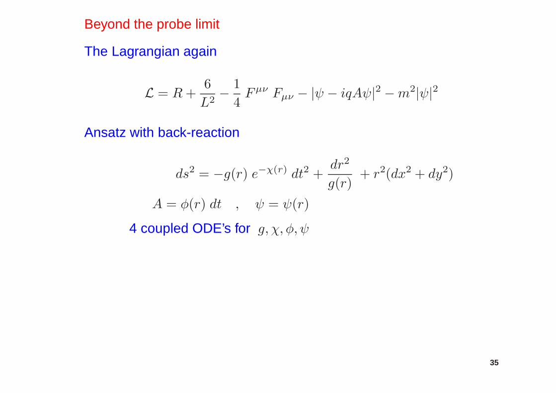
Beyond the probe limit

The Lagrangian again

L = R+6

L2− 1

4Fµν Fµν − |ψ − iqAψ|2 −m2|ψ|2

Ansatz with back-reaction

ds2 = −g(r) e−χ(r) dt2 +dr2

g(r)+ r2(dx2 + dy2)

A = φ(r) dt , ψ = ψ(r)

4 coupled ODE’s for g, χ, φ, ψ

35

Two scaling symmetries:

1) t→ at , eχ → a2eχ , φ→ φ/a

2) r → ar , (t, x, y)→ 1a(t, x, y) , g → a2g , φ→ aφ

from 1) : set χ = 0 for r →∞from 2) : set r0 = 1 (provided T 6= 0)

Two main differences in numerical solution

• A divergence in the probe limit of <O1>Tc

for T → 0 disappearsnow

36

• For m2 close to BF bound, Tc remains nonzero even when chargeof condensate q = 0.

New instability of near extremal charged AdS b.h. to forming neutralscalar hair.

37

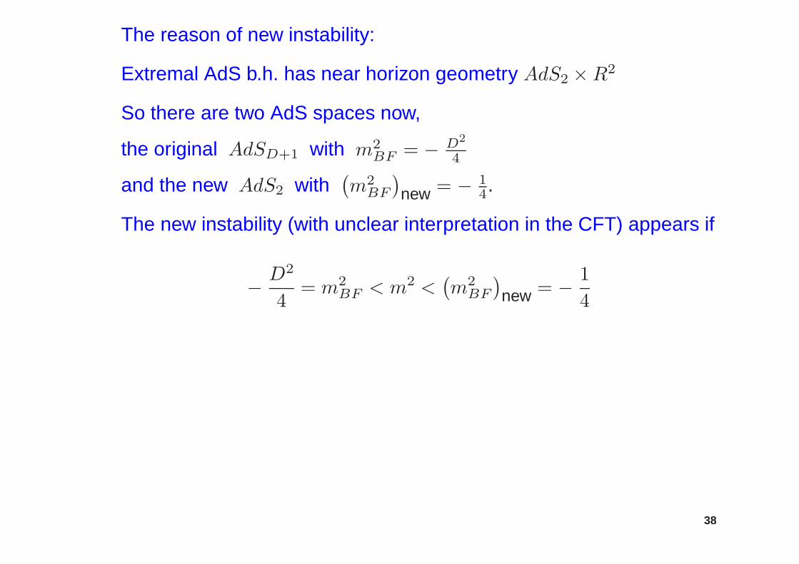
The reason of new instability:

Extremal AdS b.h. has near horizon geometry AdS2 ×R2

So there are two AdS spaces now,

the original AdSD+1 with m2BF = − D2

4

and the new AdS2 with(m2

BF

)

new = − 14.

The new instability (with unclear interpretation in the CFT) appears if

− D2

4= m2

BF < m2 <(m2

BF

)

new = − 1

4

38

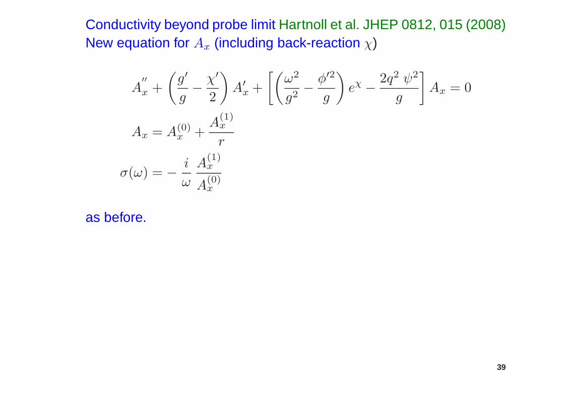
Conductivity beyond probe limit Hartnoll et al. JHEP 0812, 015 (2008)New equation for Ax (including back-reaction χ)

A′′x +

(g′

g− χ

′

2

)

A′x +

[(ω2

g2− φ

′2

g

)

eχ − 2q2 ψ2

g

]

Ax = 0

Ax = A(0)x +

A(1)x

r

σ(ω) = − i

ω

A(1)x

A(0)x

as before.

39

A more transparent way to get the conductivity

New radial variable

dz =eχ/2

gdr

Near horizon (where g ∼ r − r0→ 0) z ∼ log (r − r0)

Asymptotically r →∞ z = −1r

Equation for Ax now looks like 1-d Schrodinger equation

−∂2z Ax + V (z)Ax = ω2Ax

potential V (z) = g[(∂r φ)

2 + 2q2 ψ2 e−χ]

• at horizon r = r0 z → −∞ : V → 0 exponentially

• asymptotically z → 0 : V ∼ z2(∆−1)

40

41

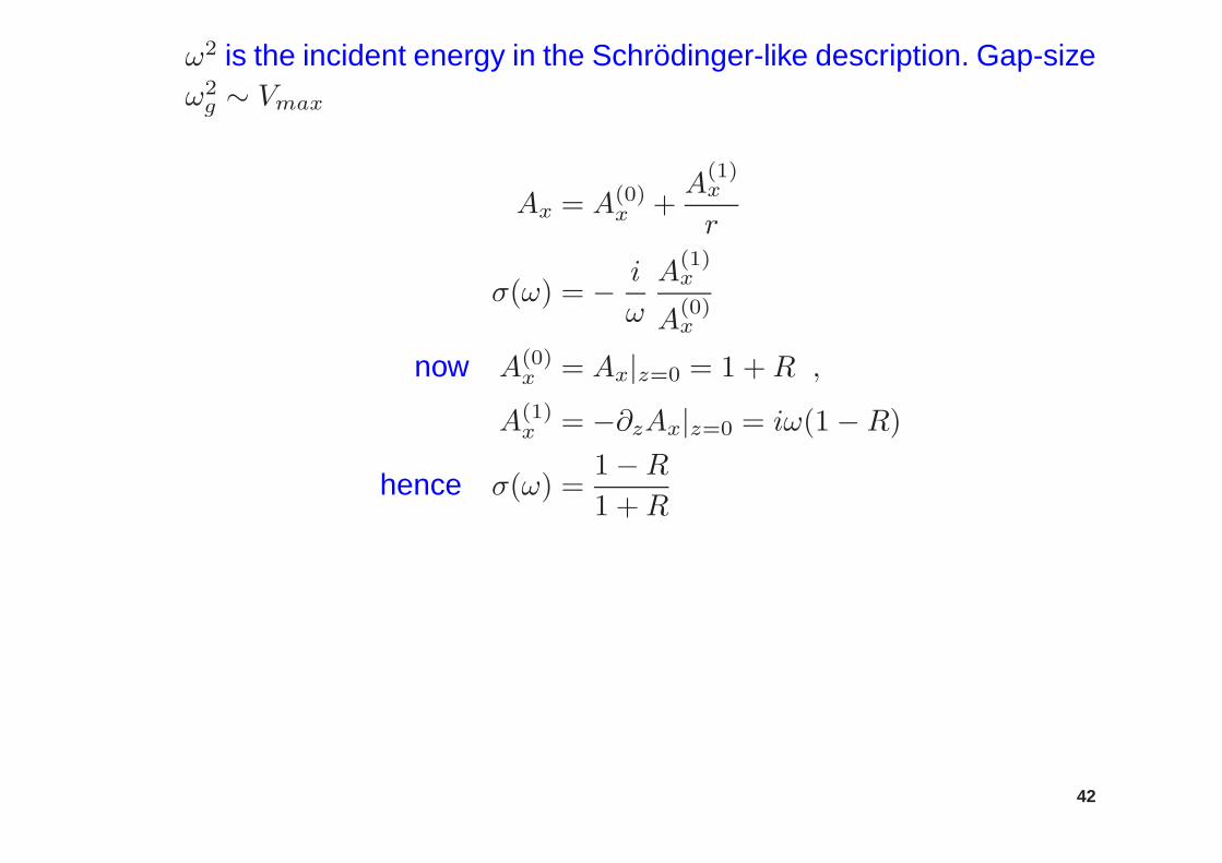
ω2 is the incident energy in the Schrodinger-like description. Gap-sizeω2g ∼ Vmax

Ax = A(0)x +

A(1)x

r

σ(ω) = − i

ω

A(1)x

A(0)x

now A(0)x = Ax|z=0 = 1 +R ,

A(1)x = −∂zAx|z=0 = iω(1− R)

hence σ(ω) =1−R1 +R

42

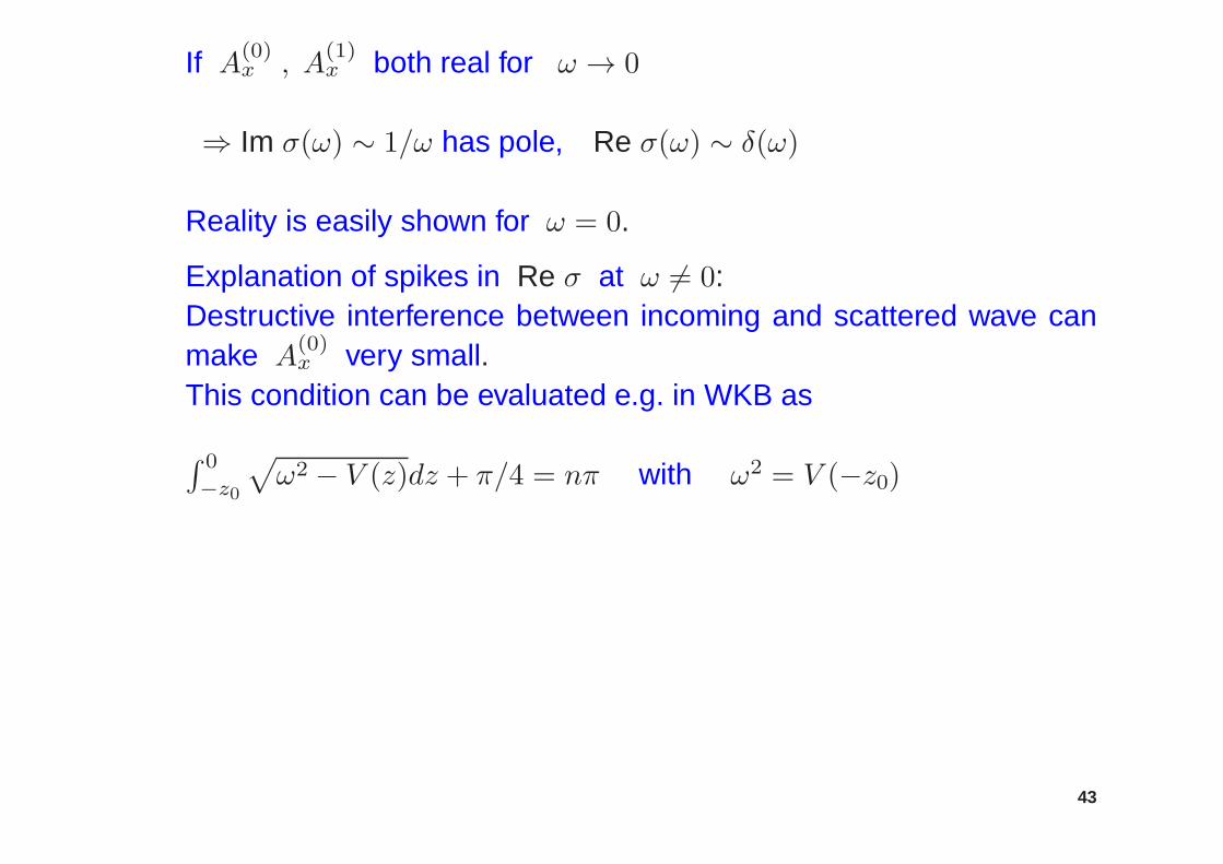
If A(0)x , A

(1)x both real for ω → 0

⇒ Im σ(ω) ∼ 1/ω has pole, Re σ(ω) ∼ δ(ω)

Reality is easily shown for ω = 0.

Explanation of spikes in Re σ at ω 6= 0:Destructive interference between incoming and scattered wave canmake A

(0)x very small.

This condition can be evaluated e.g. in WKB as

∫ 0

−z0

√

ω2 − V (z)dz + π/4 = nπ with ω2 = V (−z0)

43

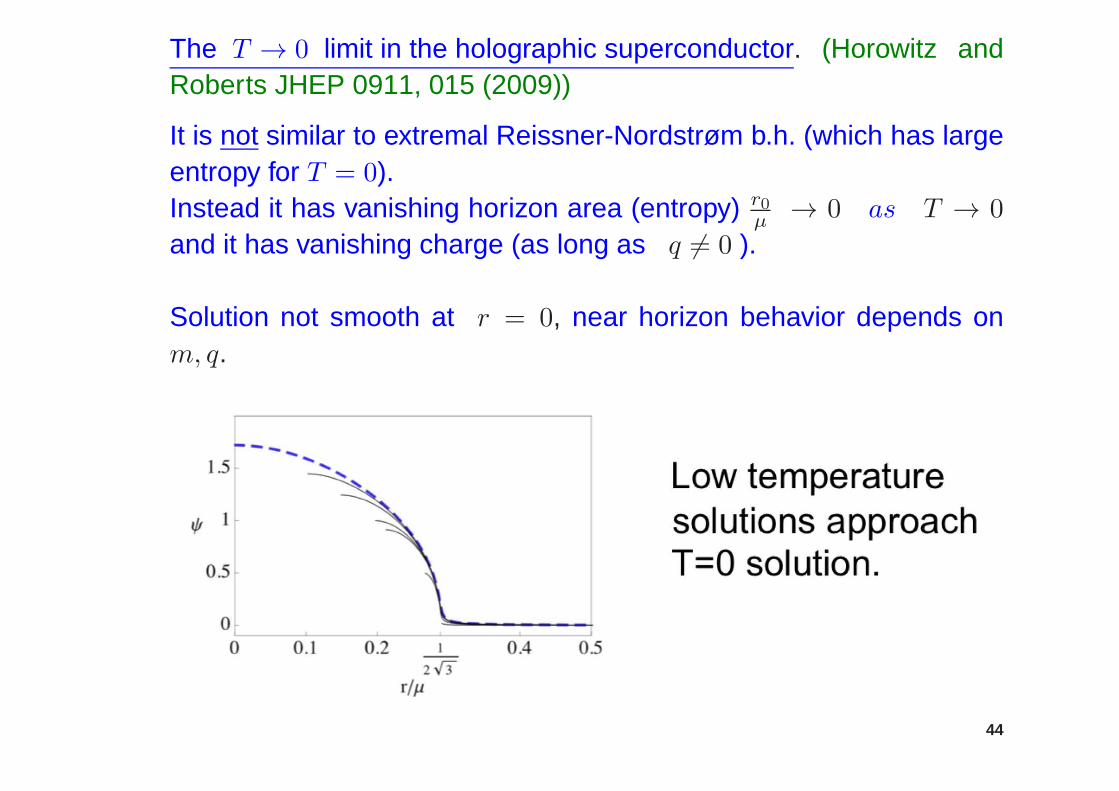
The T → 0 limit in the holographic superconductor. (Horowitz andRoberts JHEP 0911, 015 (2009))

It is not similar to extremal Reissner-Nordstrøm b.h. (which has largeentropy for T = 0).Instead it has vanishing horizon area (entropy) r0

µ → 0 as T → 0

and it has vanishing charge (as long as q 6= 0 ).

Solution not smooth at r = 0, near horizon behavior depends onm, q.

44

V (z) = 0 at horizon z → −∞ still holds

hence there is always a transmitted wave in the scattering description,

and Re σ(ω) 6= 0 for small ω also at T = 0 and

there is never a sharp gap, even at T = 0.

V (z) ∼ 1

z2near horizon

0∫

−∞

√

V (z) dz =∞

limω→0

Re σ(ω)∣∣∣T=0

= 0

45

Adding magnetic fields

If (Work to expell applied magnetic field B) > Fnormal − Fsupercond.then superconductivity is destroyed:

B2c(T )V

8π= Fn(T )− Fsc(T )

First order transition at B = Bc type I superconductor

second order transition at B = Bc : type II

The holographic superconductor turns out as type II.

In D= 3 = 2+1 dimensions Bc(T ) = 0.46

47