71
Advanced Algorithms Advanced Algorithms Piyush Kumar Piyush Kumar (Lecture 10: Compression) (Lecture 10: Compression) Welcome to COT5405 Source: Guy E. Blelloch, Emad, Tseng …
| Date post: | 26-Dec-2015 |
| Category: |
Documents |
| Upload: | baldwin-morrison |
| View: | 218 times |
| Download: | 0 times |

Advanced AlgorithmsAdvanced AlgorithmsAdvanced AlgorithmsAdvanced Algorithms
Piyush KumarPiyush Kumar(Lecture 10: Compression)(Lecture 10: Compression)
Welcome to COT5405 Source: Guy E. Blelloch,Emad, Tseng …

Compression Programs• File Compression: Gzip, Bzip• Archivers :Arc, Pkzip, Winrar, …• File Systems: NTFS
Multimedia• HDTV (Mpeg 4)• Sound (Mp3)• Images (Jpeg)

Compression OutlineIntroduction: Lossy vs. LosslessInformation Theory: Entropy, etc.Probability Coding: Huffman +
Arithmetic Coding

Encoding/Decoding
Encoder Decoder
Will use “message” in generic sense to mean the data to be compressed
InputMessage
OutputMessage
CompressedMessage
The encoder and decoder need to understand common compressed format.
CODEC

Lossless vs. LossyLossless: Input message = Output message
Lossy: Input message Output message
Lossy does not necessarily mean loss of quality. In fact the output could be “better” than the input.– Drop random noise in images (dust on lens)– Drop background in music– Fix spelling errors in text. Put into better form.
Writing is the art of lossy text compression.

Lossless Compression Techniques
• LZW (Lempel-Ziv-Welch) compression– Build dictionary– Replace patterns with index of dict.
• Burrows-Wheeler transform– Block sort data to improve compression
• Run length encoding– Find & compress repetitive sequences
• Huffman code– Use variable length codes based on frequency

How much can we compress?
For lossless compression, assuming all input messages are valid, if even one string is compressed, some other must expand.

Model vs. Coder
To compress we need a bias on the probability of messages. The model determines this bias
Example models:– Simple: Character counts, repeated strings– Complex: Models of a human face
Model CoderProbs. BitsMessages
Encoder

Quality of Compression
Runtime vs. Compression vs. GeneralitySeveral standard corpuses to compare algorithmsCalgary Corpus• 2 books, 5 papers, 1 bibliography,
1 collection of news articles, 3 programs, 1 terminal session, 2 object files, 1 geophysical data, 1 bitmap bw image
The Archive Comparison Test maintains a comparison of just about all algorithms publicly available

Comparison of Algorithms
Program Algorithm Time BPC Score
BOA PPM Var. 94+97 1.91 407
PPMD PPM 11+20 2.07 265
IMP BW 10+3 2.14 254
BZIP BW 20+6 2.19 273
GZIP LZ77 Var. 19+5 2.59 318
LZ77 LZ77 ? 3.94 ?
Information TheoryAn interface between modeling and
coding• Entropy
– A measure of information content
• Entropy of the English Language– How much information does each
character in “typical” English text contain?

Entropy (Shannon 1948)
For a set of messages S with probability p(s), s S, the self information of s is:
Measured in bits if the log is base 2.
The lower the probability, the higher the information
Entropy is the weighted average of self information.
H S p sp ss S
( ) ( ) log( )
1
i sp s
p s( ) log( )
log ( ) 1

Entropy Example
p S( ) {. ,. ,. ,. ,. } 25 25 25 125 125
H S( ) . log . log . 3 25 4 2 125 8 2 25
p S( ) {. ,. ,. ,. ,. } 5 125 125 125 125
p S( ) {. ,. ,. ,. ,. } 75 0625 0625 0625 0625
H S( ) . log . log 5 2 4 125 8 2
H S( ) . log( ) . log . 75 4 3 4 0625 16 13

Entropy of the English LanguageHow can we measure the information per character?
ASCII code = 7Entropy = 4.5 (based on character probabilities)Huffman codes (average) = 4.7Unix Compress = 3.5Gzip = 2.5BOA = 1.9 (current close to best text compressor)
Must be less than 1.9.

Shannon’s experimentAsked humans to predict the next character
given the whole previous text. He used these as conditional probabilities to estimate the entropy of the English Language.
The number of guesses required for right answer:
From the experiment he predicted H(English) = .6-1.3
# of guesses 1 2 3 3 5 > 5Probability .79 .08 .03 .02 .02 .05

Data compression model
Reduce Data Redundancy
Reduction of Entropy
Entropy Encoding
Input data
Compressed Data

CodingHow do we use the probabilities to
code messages?• Prefix codes and relationship to
Entropy• Huffman codes• Arithmetic codes• Implicit probability codes…

Assumptions
Communication (or file) broken up into pieces called messages.
Adjacent messages might be of a different types and come from a different probability distributions
We will consider two types of coding:• Discrete: each message is a fixed set of bits
– Huffman coding, Shannon-Fano coding• Blended: bits can be “shared” among messages
– Arithmetic coding

Uniquely Decodable Codes
A variable length code assigns a bit string (codeword) of variable length to every message value
e.g. a = 1, b = 01, c = 101, d = 011What if you get the sequence of bits1011 ?
Is it aba, ca, or, ad?A uniquely decodable code is a variable
length code in which bit strings can always be uniquely decomposed into its codewords.

Prefix CodesA prefix code is a variable length
code in which no codeword is a prefix of another word
e.g a = 0, b = 110, c = 111, d = 10Can be viewed as a binary tree with
message values at the leaves and 0 or 1s on the edges.
a
b c
d
0
0
0 1
1
1

Some Prefix Codes for Integers
n Binary Unary Split
1 ..001 0 1|
2 ..010 10 10|0
3 ..011 110 10|1
4 ..100 1110 110|00
5 ..101 11110 110|01
6 ..110 111110 110|10
Many other fixed prefix codes: Golomb, phased-binary, subexponential, ...

Average Bit LengthFor a code C with associated probabilities
p(c) the average length is defined as
We say that a prefix code C is optimal if for all prefix codes C’,
ABL(C) ABL(C’)
Cc
clcpCABL )()()(

Relationship to EntropyTheorem (lower bound): For any
probability distribution p(S) with associated uniquely decodable code C,
Theorem (upper bound): For any probability distribution p(S) with associated optimal prefix code C,
)()( CABLSH
1)()( SHCABL

Kraft McMillan Inequality
Theorem (Kraft-McMillan): For any uniquely decodable code C,
Also, for any set of lengths L such that
there is a prefix code C such that
2 1
l c
c C
( )
2 1
l
l L
l c l i Li i( ) ( ,...,| |) 1
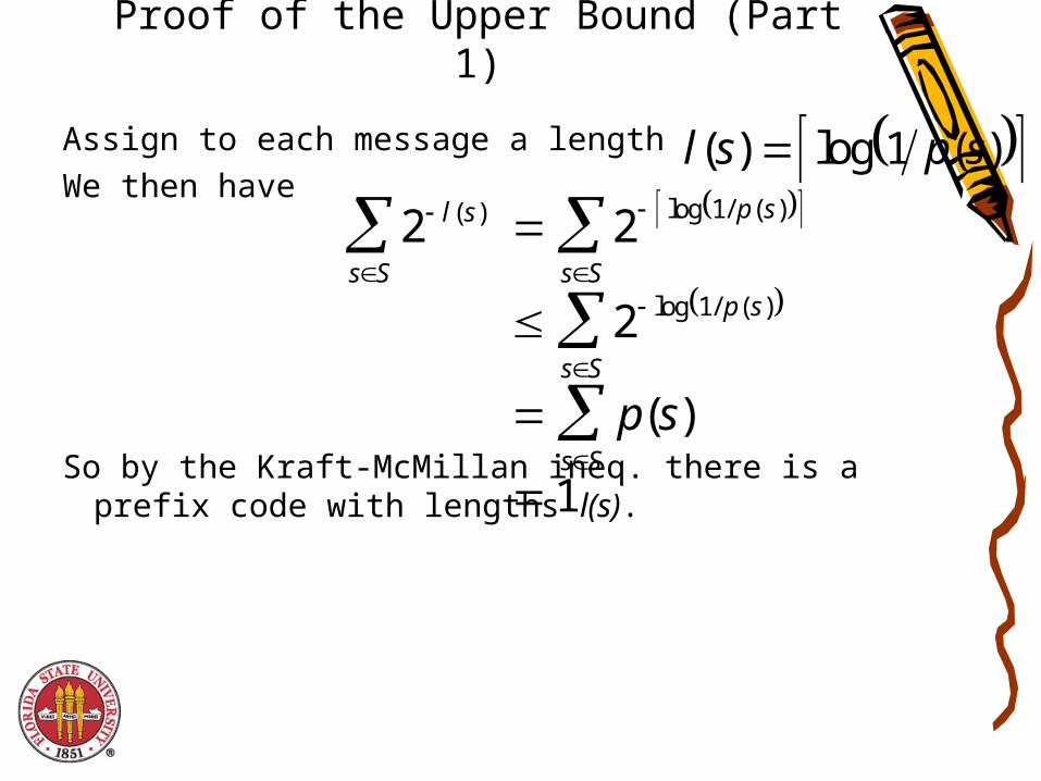
Proof of the Upper Bound (Part 1)
Assign to each message a lengthWe then have
So by the Kraft-McMillan ineq. there is a prefix code with lengths l(s).
l s p s( ) log ( ) 1
2 2
2
1
1
1
l s
s S
p s
s Sp s
s S
s S
p s
( ) log / ( )
log / ( )
( )

Proof of the Upper Bound (Part 2)
)(1
))(/1log()(1
)))(/1log(1()(
)(/1log)(
)()()(
SH
spsp
spsp
spsp
slspSABL
Ss
Ss
Ss
Ss
Now we can calculate the average length given l(s)
And we are done.

Another property of optimal codes
Theorem: If C is an optimal prefix code for the probabilities {p1, …, pn} then pi < pj implies l(ci) l(ci)
Proof: (by contradiction)Assume l(ci) < l(cj). Consider switching codes ci and cj. If la is the average length of the original code, the length of the new code is
This is a contradiction since la was supposed to be optimal
l l p l c l c p l c l cl p p l c l cl
a a j i j i j i
a j i i j
a
' ( ( ) ( )) ( ( ) ( ))( )( ( ) ( ))

Corollary• The pi is smallest over the code, then
l(ci) is the largest.

Huffman CodingHuffman CodingHuffman CodingHuffman Coding
Binary trees for compressionBinary trees for compression

Huffman Code• Approach
– Variable length encoding of symbols– Exploit statistical frequency of symbols– Efficient when symbol probabilities vary widely
• Principle– Use fewer bits to represent frequent symbols – Use more bits to represent infrequent symbols
A A B A
A AA B

Huffman CodesInvented by Huffman as a class assignment in
1950.Used in many, if not most compression algorithms
• gzip, bzip, jpeg (as option), fax compression,…
Properties:– Generates optimal prefix codes– Cheap to generate codes– Cheap to encode and decode
– la=H if probabilities are powers of 2

Huffman Code Example
• Expected size– Original 1/82 + 1/42 + 1/22 + 1/82 = 2 bits / symbol– Huffman 1/83 + 1/42 + 1/21 + 1/83 = 1.75 bits / symbol
Symbol Dog Cat Bird Fish
Frequency 1/8 1/4 1/2 1/8
Original Encoding
00 01 10 11
2 bits 2 bits 2 bits 2 bits
Huffman Encoding
110 10 0 111
3 bits 2 bits 1 bit 3 bits

Huffman CodesHuffman Algorithm• Start with a forest of trees each consisting of
a single vertex corresponding to a message s and with weight p(s)
• Repeat:– Select two trees with minimum weight roots p1 and
p2
– Join into single tree by adding root with weight p1 + p2

Example
p(a) = .1, p(b) = .2, p(c ) = .2, p(d) = .5
a(.1) b(.2) d(.5)c(.2)
a(.1) b(.2)
(.3)
a(.1) b(.2)
(.3) c(.2)
a(.1) b(.2)
(.3) c(.2)
(.5)
(.5) d(.5)
(1.0)
a=000, b=001, c=01, d=1
0
0
0
1
1
1Step 1
Step 2Step 3

Encoding and DecodingEncoding: Start at leaf of Huffman tree
and follow path to the root. Reverse order of bits and send.
Decoding: Start at root of Huffman tree and take branch for each bit received. When at leaf can output message and return to root.
a(.1) b(.2)
(.3) c(.2)
(.5) d(.5)
(1.0)0
0
0
1
1
1
There are even faster methods that can process 8 or 32 bits at a time
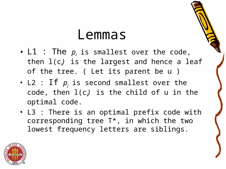
Lemmas• L1 : The pi is smallest over the code, then
l(ci) is the largest and hence a leaf of the tree. ( Let its parent be u )
• L2 : If pj is second smallest over the code, then l(ci) is the child of u in the optimal code.
• L3 : There is an optimal prefix code with corresponding tree T*, in which the two lowest frequency letters are siblings.

Huffman codes are optimal
Theorem: The Huffman algorithm generates an optimal prefix code.
In other words: It achieves the minimum average number of bits per letter of any prefix code.
Proof: By inductionBase Case: Trivial (one bit optimal)Assumption: The method is optimal for
all alphabets of size k-1.

Proof:• Let y* and z* be the two lowest
frequency letters merged in w*. Let T be the tree before merging and T’ after merging.
• Then : ABL(T’) = ABL(T) – p(w*)• T’ is optimal by induction.

Proof:• Let Z be a better tree compared to T
produced using Huffman’s alg.• Implies ABL(Z) < ABL(T)• By lemma L3, there is such a tree Z’ in
which the leaves representing y* and z* are siblings (and has same ABL as Z).
• By previous page ABL(Z’) =ABL(Z) – p(w*)
• Contradiction!

Adaptive Huffman Codes
Huffman codes can be made to be adaptive without completely recalculating the tree on each step.
• Can account for changing probabilities• Small changes in probability, typically
make small changes to the Huffman tree
Used frequently in practice
Huffman Coding Disadvantages
• Integral number of bits in each code.
• If the entropy of a given character is 2.2 bits,the Huffman code for that character must be either 2 or 3 bits , not 2.2.

Towards Arithmetic coding
• An Example: Consider sending a message of length 1000 each with having probability .999
• Self information of each message -log(.999)= .00144 bits• Sum of self information = 1.4 bits.• Huffman coding will take at least 1k bits.• Arithmetic coding = 3 bits!

Arithmetic Coding: Introduction
Allows “blending” of bits in a message sequence.
Can bound total bits required based on sum of self information:
Used in PPM, JPEG/MPEG (as option), DMMMore expensive than Huffman coding, but integer
implementation is not too bad.
l sii
n
2
1

Arithmetic Coding (message intervals)
Assign each probability distribution to an interval range from 0 (inclusive) to 1 (exclusive).
e.g.
a = .2
c = .3
b = .5
f(a) = .0, f(b) = .2, f(c) = .7
f i p jj
i
( ) ( )
1
1
The interval for a particular message will be calledthe message interval (e.g for b the interval is [.2,.7))

Arithmetic Coding (sequence intervals)
To code a message use the following:
Each message narrows the interval by a factor of pi.
Final interval size:
The interval for a message sequence will be called the sequence interval
l f l l s fs p s s p
i i i i
i i i
1 1 1 1
1 1 1
s pn ii
n
1

Arithmetic Coding: Encoding Example
Coding the message sequence: bac
The final interval is [.27,.3)
a = .2
c = .3
b = .5
0.0
0.2
0.7
1.0
a = .2
c = .3
b = .5
0.2
0.3
0.55
0.7
a = .2
c = .3
b = .5
0.2
0.21
0.27
0.3

Uniquely defining an interval
Important property:The sequence intervals for distinct message sequences of length n will never overlap
Therefore: specifying any number in the final interval uniquely determines the sequence.
Decoding is similar to encoding, but on each step need to determine what the message value is and then reduce interval
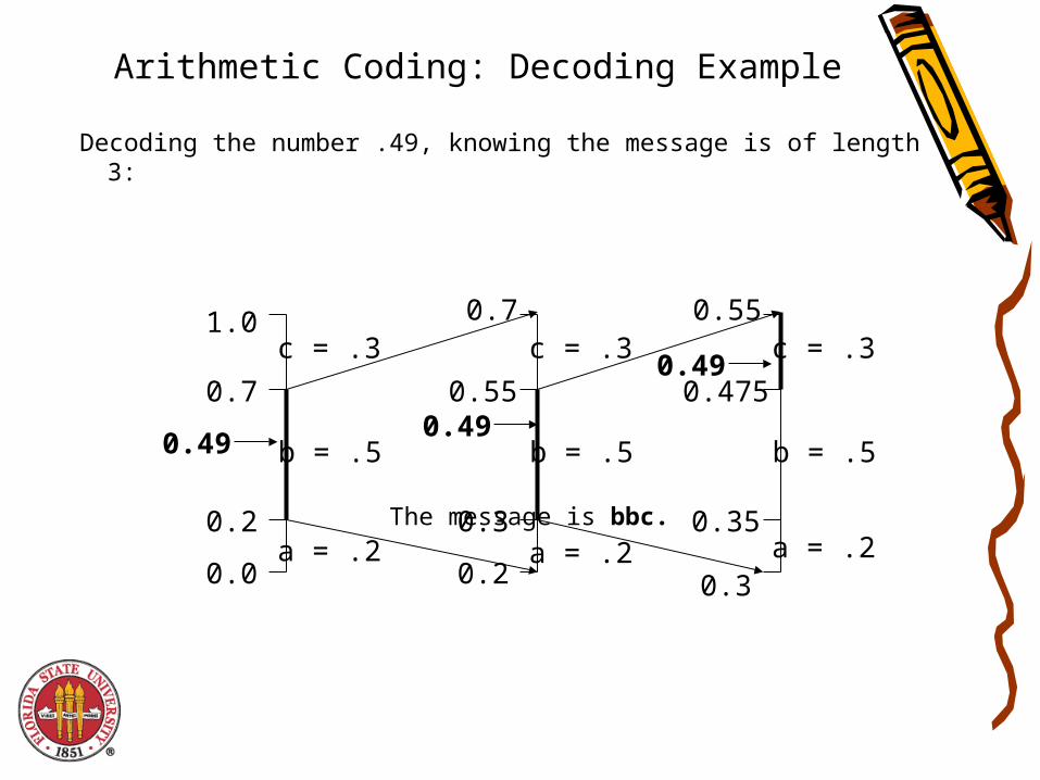
Arithmetic Coding: Decoding Example
Decoding the number .49, knowing the message is of length 3:
The message is bbc.a = .2
c = .3
b = .5
0.0
0.2
0.7
1.0
a = .2
c = .3
b = .5
0.2
0.3
0.55
0.7
a = .2
c = .3
b = .5
0.3
0.35
0.475
0.55
0.490.49
0.49

Representing an Interval
Binary fractional representation:
So how about just using the smallest binary fractional representation in the sequence interval. e.g. [0,.33) = .01 [.33,.66) = .1 [.66,1) = .11
But what if you receive a 1? Is the code complete? (Not a prefix code)
. .
/ .
/ .
75 11
1 3 0101
11 16 1011

Representing an Interval (continued)
Can view binary fractional numbers as intervals by considering all completions. e.g.
We will call this the code interval.Lemma: If a set of code intervals do not overlap then the
corresponding codes form a prefix code.
min max interval
. . . [. , . )
. . . [. ,. )
11 110 111 75 10
101 1010 1011 625 75

Selecting the Code IntervalTo find a prefix code find a binary fractional number whose
code interval is contained in the sequence interval.
e.g. [0,.33) = .00 [.33,.66) = .100 [.66,1) = .11Can use l + s/2 truncated to
bits
.61
.79
.625
.75Sequence Interval Code Interval (.101)
log( ) logs s2 1

RealArith Encoding and Decoding
RealArithEncode:• Determine l and s using original recurrences• Code using l + s/2 truncated to 1+-log s bitsRealArithDecode:• Read bits as needed so code interval falls
within a message interval, and then narrow sequence interval.
• Repeat until n messages have been decoded .

Bound on Length
Theorem: For n messages with self information {s1,…,sn} RealArithEncode will generate at most
bits.
1 1
1
1
2
1
1
1
1
log log
log
s p
p
s
s
ii
n
ii
n
ii
n
ii
n
21
sii
n

Integer Arithmetic Coding
Problem with RealArithCode is that operations on arbitrary precision real numbers is expensive.
Key Ideas of integer version:• Keep integers in range [0..R) where R=2k
• Use rounding to generate integer interval• Whenever sequence intervals falls into top,
bottom or middle half, expand the interval by factor of 2 Integer Algorithm is an approximation

Applications of Probability Coding
How do we generate the probabilities?Using character frequencies directly does not work very
well (e.g. 4.5 bits/char for text).Technique 1: transforming the data• Run length coding (ITU Fax standard)• Move-to-front coding (Used in Burrows-Wheeler)• Residual coding (JPEG LS)Technique 2: using conditional probabilities• Fixed context (JBIG…almost)• Partial matching (PPM)

Run Length CodingCode by specifying message value
followed by number of repeated values:e.g. abbbaacccca => (a,1),(b,3),(a,2),
(c,4),(a,1)The characters and counts can be coded
based on frequency.This allows for small number of bits
overhead for low counts such as 1.

Facsimile ITU T4 (Group 3)
Standard used by all home Fax MachinesITU = International Telecommunications StandardRun length encodes sequences of black+white pixels
Fixed Huffman Code for all documents. e.g.
Since alternate black and white, no need for values.
Run length White Black
1 000111 010
2 0111 11
10 00111 0000100

Move to Front CodingTransforms message sequence into sequence of
integers, that can then be probability codedStart with values in a total order:
e.g.: [a,b,c,d,e,….]For each message output position in the order and
then move to the front of the order.e.g.: c => output: 3, new order: [c,a,b,d,e,…] a => output: 2, new order: [a,c,b,d,e,…]
Codes well if there are concentrations of message values in the message sequence.

Residual CodingUsed for message values with
meaningfull ordere.g. integers or floats.
Basic Idea: guess next value based on current context. Output difference between guess and actual value. Use probability code on the output.

JPEG-LSJPEG Lossless (not to be confused with lossless
JPEG)Just completed standardization process.
Codes in Raster Order. Uses 4 pixels as context:
Tries to guess value of * based on W, NW, N and NE.
Works in two stages
NW
W
N NE
*

JPEG LS: Stage 1
Uses the following equation:
Averages neighbors and captures edges. e.g.
otherwise
),min( if),max(
),max( if),min(
NWWN
WNNWWN
WNNWWN
P
40
40
3 *
30
20
40 *
3
40
3 *

JPEG LS: Stage 2Uses 3 gradients: W-NW, NW-N, N-NE• Classifies each into one of 9 categories.• This gives 93=729 contexts, of which only 365
are needed because of symmetry.• Each context has a bias term that is used to
adjust the previous predictionAfter correction, the residual between guessed
and actual value is found and coded using a Golomblike code.

Using Conditional Probabilities: PPM
Use previous k characters as the context.Base probabilities on counts:
e.g. if seen th 12 times followed by e 7 times, then the conditional probability p(e|th)=7/12.
Need to keep k small so that dictionary does not get too large.

Ideas in Lossless compression
• That we did not talk about specifically– Lempel-Ziv (gzip)
• Tries to guess next window from previous data
– Burrows-Wheeler (bzip)• Context sensitive sorting• Block sorting transform

LZ77: Sliding Window Lempel-Ziv
Dictionary and buffer “windows” are fixed length and slide with the cursor
On each step:• Output (p,l,c)
p = relative position of the longest match in the dictionaryl = length of longest matchc = next char in buffer beyond longest match
• Advance window by l + 1
a a c a a c a b c a b a b a cDictionary
(previously coded)Lookahead
Buffer
Cursor

Lossy compression
Scalar Quatization• Given a camera image with 12bit
color, make it 4-bit grey scale.• Uniform Vs Non-Uniform
Quantization– The eye is more sensitive to low
values of red compared to high values.
Vector Quantization• How do we compress a color
image (r,g,b)?– Find k – representative points for all
colors– For every pixel, output the nearest
representative– If the points are clustered around the
representatives, the residuals are small and hence probability coding will work well.
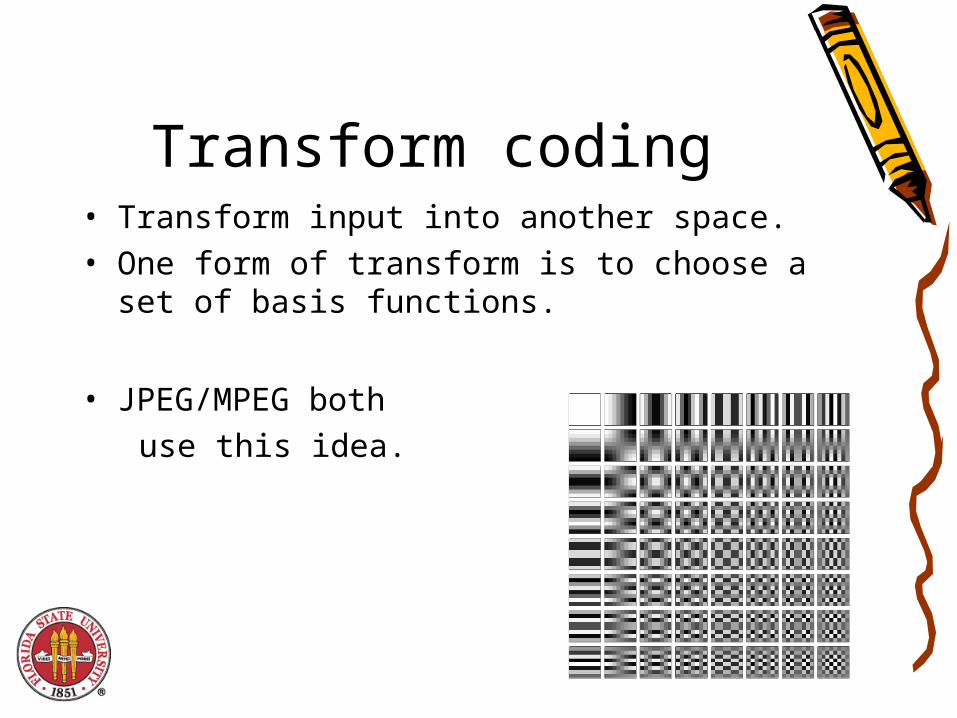
Transform coding• Transform input into another space.• One form of transform is to choose a set of
basis functions.
• JPEG/MPEG both use this idea.

Other Transform codes• Wavelets• Fractal base compression
– Based on the idea of fixed points of functions.


