woodplc.com

Advanced analysis foroffshore windinter-array cables

Keith AndersonSubsea and export systems manager

2

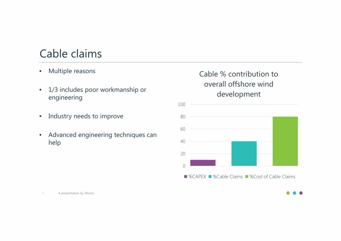
Cable claims• Multiple reasons

• 1/3 includes poor workmanship orengineering

• Industry needs to improve

• Advanced engineering techniques canhelp

3 A presentation by Wood.

0

20

40

60

80

100

Cable % contribution tooverall offshore wind

development

%CAPEX %Cable Claims %Cost of Cable Claims

• Cable protection system engineering

• Freespan analysis

• Local cross-section modeling

• Conclusion

Scope of presentation

4 A presentation by Wood.

5

Cable protection system advanced analysis

• Cable hang-off at platform level

• Cable entry location near seabed

• Cable protection options– Internal to monopile

• Internal J-tube• Internal guides• Free hanging• If J-tubes are not used bend protection

required

– External to monopile• J-tube• Bend protection system

Cable entry systems for monopilesOverview

6 A presentation by Wood.

• Cable modelled from exit to seabed

• Cable exit point:– Axially fixed point– Rotational motions permitted up to constraints

• Cable and ancillary protection equipment modelledas equivalent beam– Combined stiffness– Combined weight

• Cables highly dynamic– High lateral deflections– Limited overlength to accommodate motion– Load transferred to burial and cable entry point

Basic system modelling – option 1 (split model)

7 A presentation by Wood.

Case study• Cable - 150mm diameter; dry weight 40kg/m• Current speed 2m/s; 100yr wave

External cable model

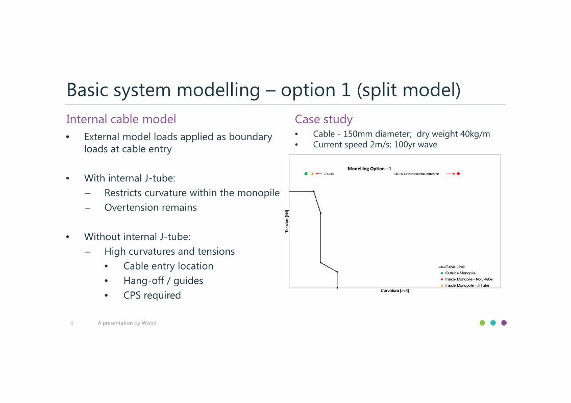
• External model loads applied as boundaryloads at cable entry

• With internal J-tube:– Restricts curvature within the monopile– Overtension remains

• Without internal J-tube:– High curvatures and tensions

• Cable entry location• Hang-off / guides• CPS required

Basic system modelling – option 1 (split model)Internal cable model

8 A presentation by Wood.

Case study• Cable - 150mm diameter; dry weight 40kg/m• Current speed 2m/s; 100yr wave

• Ancillary equipment modelledindependently from cable– Pipe in pipe contact modelling– No axial load transfer– Allows relative CPS / cable

movement

• Improved external system loads at thecable entry point

• Reduced input loads to internal modelimproves the curvatures within themonopile– Less onerous CPS requirements

Intermediate modelling – option 2 (split model PiP)Independent CPS modelling

9 A presentation by Wood.

Case study• Cable - 150mm diameter; dry weight 40kg/m• Current speed 2m/s; 100yr wave

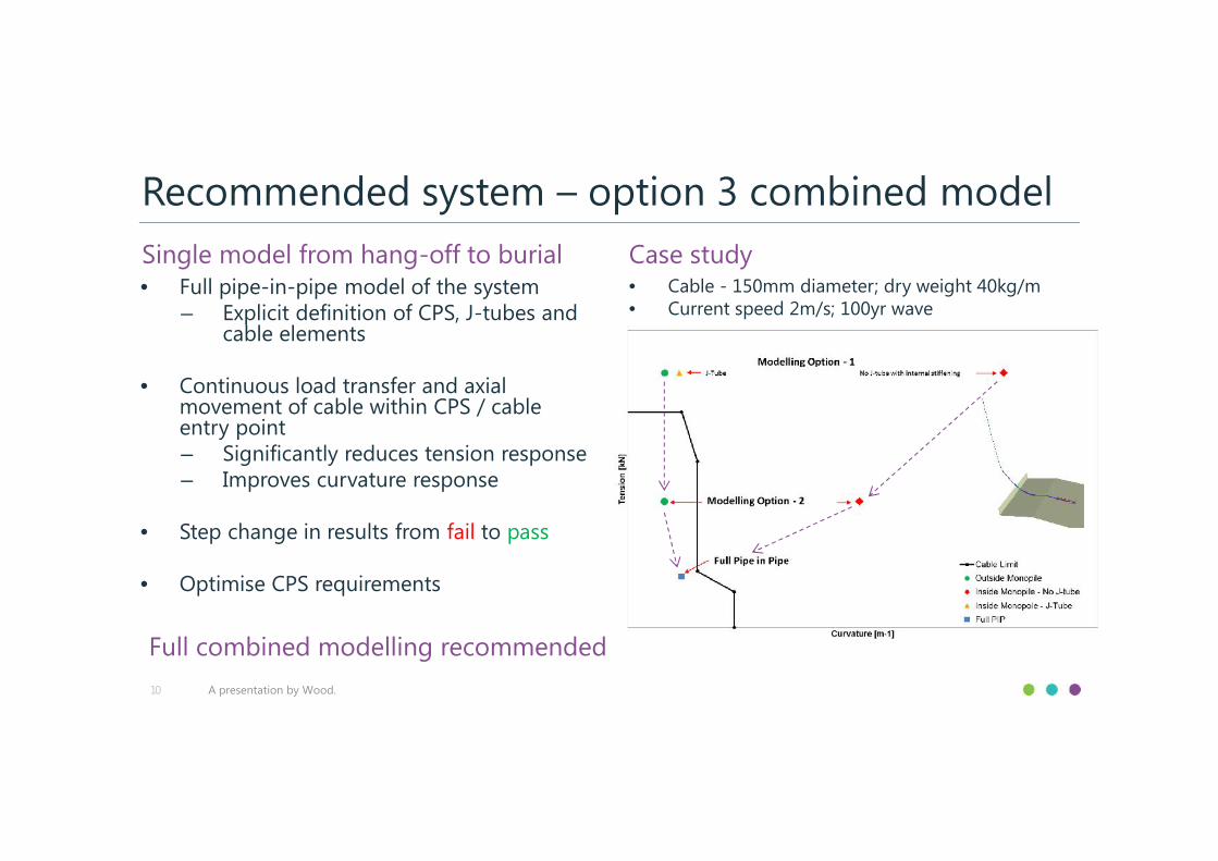
• Full pipe-in-pipe model of the system– Explicit definition of CPS, J-tubes and

cable elements

• Continuous load transfer and axialmovement of cable within CPS / cableentry point– Significantly reduces tension response– Improves curvature response

• Step change in results from fail to pass

• Optimise CPS requirements

Recommended system – option 3 combined modelSingle model from hang-off to burial

10 A presentation by Wood.

Case study• Cable - 150mm diameter; dry weight 40kg/m• Current speed 2m/s; 100yr wave

Full combined modelling recommended

11

Freespan advanced analysis

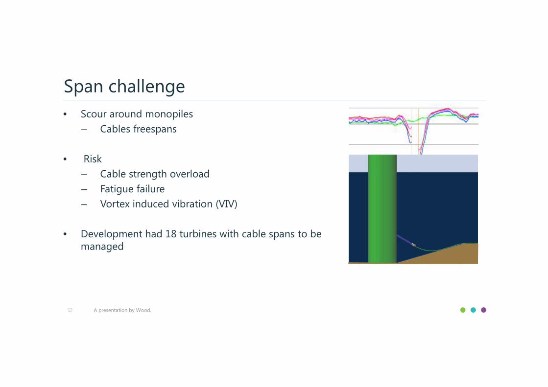
• Scour around monopiles– Cables freespans

• Risk– Cable strength overload– Fatigue failure– Vortex induced vibration (VIV)

• Development had 18 turbines with cable spans to bemanaged

Span challenge

12 A presentation by Wood.

• System modelling– Pipe in pipe modelling in J-tube– Local cross-section stress analysis

• Extreme strength– 100yr response proven within criteria

• Wave fatigue– Residual life sufficient for life of field operations

Strength and wave fatigue

13 A presentation by Wood.

• Company initial approach– 100yr peak wave velocity– Highly conservative, no VIV allowed– Multiple span mitigations required

• Wood approach– Accept VIV via engineering– Model system responses– Determine fatigue life

Advanced VIV approach

14 A presentation by Wood.

Scou

r Pit

Dep

th (m

)

Scour Pit Diameter (m)

Scour pit diameter vs depth

Survey Scour Profiles Wood Scour Profile Value

• Environmental considerations– 10% of wave scatter not applicable

• Large motion response decouples VIV• 100yr wave not applicable

– Waves and tidal cycle are oscillatory• Peak velocity not critical• Combined duration above onset velocities

• Flow normal to pipeline– Reduced effective in-plane current

Advanced VIV models

15 A presentation by Wood.

-0.6

-0.4

-0.2

0.0

0.2

0.4

0.6

0.0 2.0 4.0 6.0 8.0

Velo

city

(m/s

)

Time (s)

• Response excitation assessment– In-line VIV

• In-plane current + normal mode• Transverse current + transverse mode

– Cross flow VIV• In-plane current + transverse mode• Transverse current + normal mode

– Span length selected to mitigate cross-flow

• Fatigue analysis for all excited modes– >400yrs fatigue life predicted– VIV less onerous than wave fatigue

Advanced VIV models

16 A presentation by Wood.

• VIV limits acceptable span lengths– Extreme performance less onerous

• Allow VIV onset and manage behaviour– Allowable span lengths increased 50%– No mitigations required

• 80:20 rule– Project ended with acceptable performance achieved– Further increases in span lengths possible

• e.g. current scatter tables

VIV summary

17 A presentation by Wood.

Local cross-section advanced modelling

18

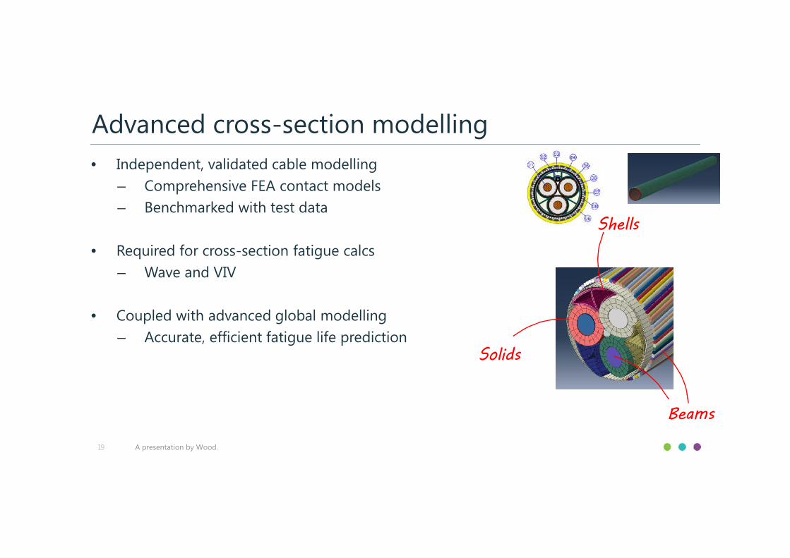
• Independent, validated cable modelling– Comprehensive FEA contact models– Benchmarked with test data

• Required for cross-section fatigue calcs– Wave and VIV

• Coupled with advanced global modelling– Accurate, efficient fatigue life prediction

Advanced cross-section modelling

19 A presentation by Wood.

Beams

Shells

Solids

Fatigue life prediction

20 A presentation by Wood.

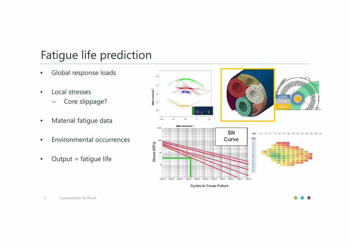
Hs (m) 4 5 6 7 8 9 10 11 12 13 14 15 16 17

Tz (s)

4 0.3 0.2 0.15 0.8 0.6 0.4 0.26 1 0.8 0.7 0.5 0.4 0.37 1.3 2 2.1 1.8 0.8 0.7 0.5 0.58 0.6 1.5 3 2 1.5 1.2 1.1 0.8 0.7 0.69 1 2 4 3.5 2 1.5 1.3 0.7 0.5 0.7 0.410 1.8 5 4.5 3.1 2.4 1.9 0.6 0.7 0.5 0.411 3 3.2 2.8 2.2 1.6 1 0.8 0.7 0.112 1 2.5 1.8 1.1 0.8 0.7 0.6 0.313 1.6 1.2 0.8 0.6 0.5 0.414 1 0.9 0.5151617

• Global response loads

• Local stresses– Core slippage?

• Material fatigue data

• Environmental occurrences

• Output = fatigue life

21

Conclusion

• Reduces conservatism in design loadings

• Supports engineering mitigation anomalies

• Enhanced fatigue life prediction

Advanced system modelling

22 A presentation by Wood.

woodplc.com