ADVANCED BUSINESS FORECASTING - NKD Group · Exponential smoothing family ... Seasonal Variation...

ADVANCED BUSINESS FORECASTING

Definition

Forecasting involves making the best possible judgment about

some future event. In other words, “forecasts are numerical

estimates of an event for some future date that can be achieved

with a specified level of support and are reproducible.”

"I often say that when you can measure what

you are speaking about, and express it in

numbers, you know something about it; but

when you cannot measure it, when you

cannot express it in numbers, your

knowledge is of a very meagre and

unsatisfactory kind."

William Thomson, Lord Kelvin, 1824-1907

"If we could first know where we are, then

whither we are tending, we could then decide

what to do and how to do it."

Abraham Lincoln, 1809-1865

The elements that come into play in all forecasting methods is

the concept of the future and time; uncertainty; and reliance on

historical data.

MELec6_6: Forecasting Page: 2

MBA555 Class Notes Prepared by: These notes contain copyrighted information Dr. Nina Kajiji Do not quote or copy without permission www.ninakajiji.net Last Update: Feb 19, 2013

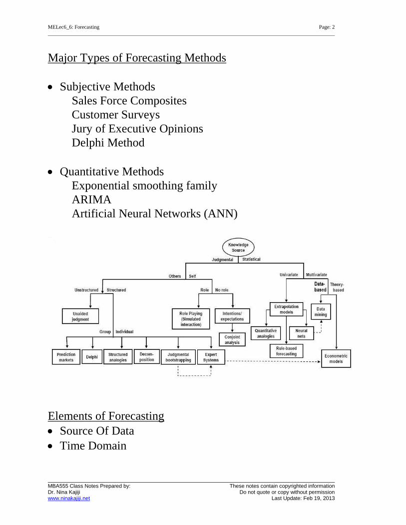
Major Types of Forecasting Methods

Subjective Methods

Sales Force Composites

Customer Surveys

Jury of Executive Opinions

Delphi Method

Quantitative Methods

Exponential smoothing family

ARIMA

Artificial Neural Networks (ANN)

Elements of Forecasting

Source Of Data

Time Domain



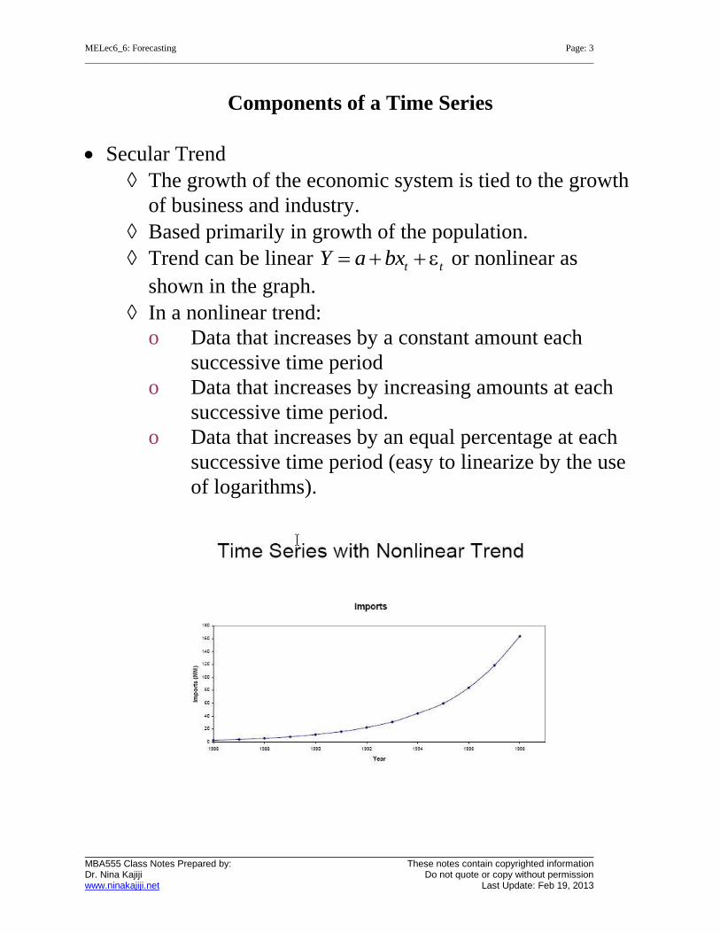
Components of a Time Series

Secular Trend

The growth of the economic system is tied to the growth

of business and industry.

Based primarily in growth of the population.

Trend can be linear t tY a bx or nonlinear as

shown in the graph.

In a nonlinear trend:

o Data that increases by a constant amount each

successive time period

o Data that increases by increasing amounts at each

successive time period.

o Data that increases by an equal percentage at each

successive time period (easy to linearize by the use

of logarithms).



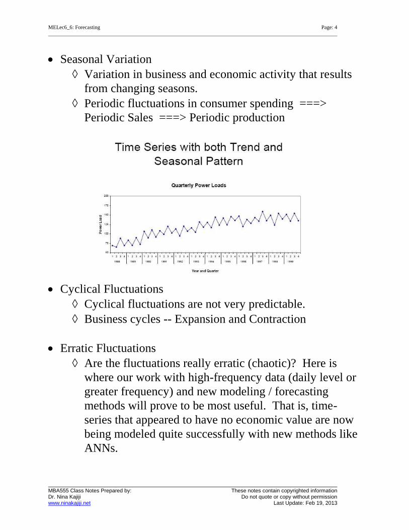
Seasonal Variation

Variation in business and economic activity that results

from changing seasons.

Periodic fluctuations in consumer spending ===>

Periodic Sales ===> Periodic production

Cyclical Fluctuations

Cyclical fluctuations are not very predictable.

Business cycles -- Expansion and Contraction

Erratic Fluctuations

Are the fluctuations really erratic (chaotic)? Here is

where our work with high-frequency data (daily level or

greater frequency) and new modeling / forecasting

methods will prove to be most useful. That is, time-

series that appeared to have no economic value are now

being modeled quite successfully with new methods like

ANNs.



Quantitative Forecasting Methods

Charting Approaches (read)

Moving average

Exponential Smoothing

Artificial Neural Networks

Charting Approaches

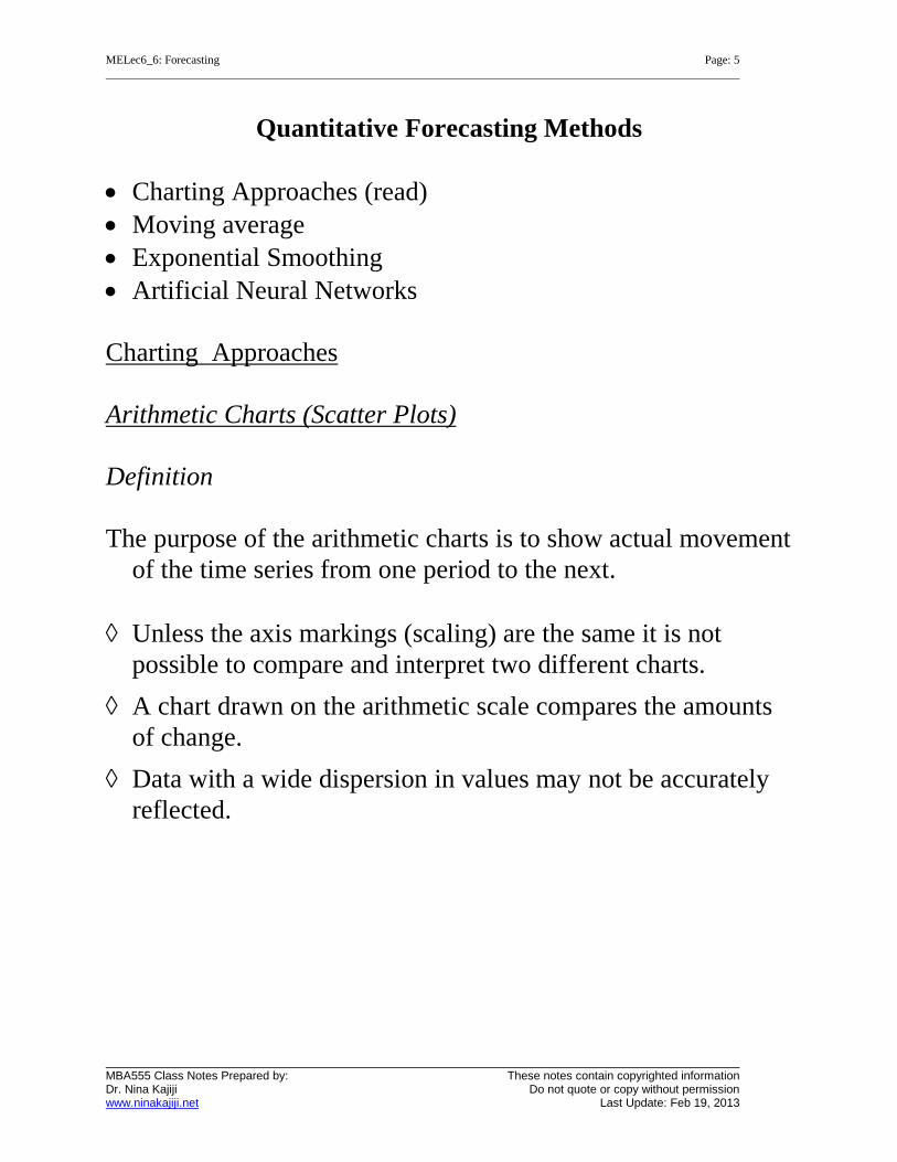
Arithmetic Charts (Scatter Plots)

Definition

The purpose of the arithmetic charts is to show actual movement

of the time series from one period to the next.

Unless the axis markings (scaling) are the same it is not

possible to compare and interpret two different charts.

A chart drawn on the arithmetic scale compares the amounts

of change.

Data with a wide dispersion in values may not be accurately

reflected.



Trade Weighted Exchange Rate

120.000

121.000

122.000

123.000

124.000

125.000

126.000

127.000

128.000

129.000

1 2 3 4 5 6 7 8 9 10 11 12 13 14 15 16 17 18 19

2001

Va

lue

Series1

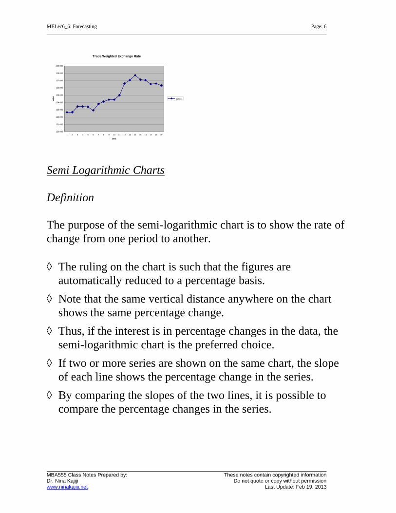
Semi Logarithmic Charts

Definition

The purpose of the semi-logarithmic chart is to show the rate of

change from one period to another.

The ruling on the chart is such that the figures are

automatically reduced to a percentage basis.

Note that the same vertical distance anywhere on the chart

shows the same percentage change.

Thus, if the interest is in percentage changes in the data, the

semi-logarithmic chart is the preferred choice.

If two or more series are shown on the same chart, the slope

of each line shows the percentage change in the series.

By comparing the slopes of the two lines, it is possible to

compare the percentage changes in the series.



Trade Weighted Exchange Rate

1.000

10.000

100.000

1000.000

1 2 3 4 5 6 7 8 9 10 11 12 13 14 15 16 17 18 19

2001

Valu

e

TWER

10%

1%

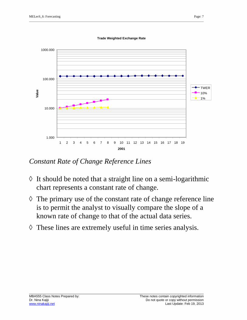
Constant Rate of Change Reference Lines

It should be noted that a straight line on a semi-logarithmic

chart represents a constant rate of change.

The primary use of the constant rate of change reference line

is to permit the analyst to visually compare the slope of a

known rate of change to that of the actual data series.

These lines are extremely useful in time series analysis.



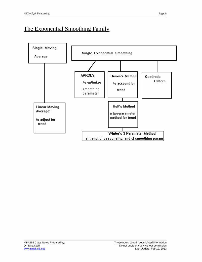
The Exponential Smoothing Family



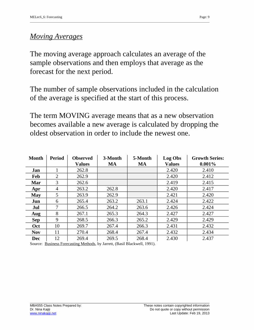
Moving Averages

The moving average approach calculates an average of the

sample observations and then employs that average as the

forecast for the next period.

The number of sample observations included in the calculation

of the average is specified at the start of this process.

The term MOVING average means that as a new observation

becomes available a new average is calculated by dropping the

oldest observation in order to include the newest one.

Month Period Observed

Values

3-Month

MA

5-Month

MA

Log Obs

Values

Growth Series:

0.001%

Jan 1 262.8 2.420 2.410

Feb 2 262.9 2.420 2.412

Mar 3 262.6 2.419 2.415

Apr 4 263.2 262.8 2.420 2.417

May 5 263.9 262.9 2.421 2.420

Jun 6 265.4 263.2 263.1 2.424 2.422

Jul 7 266.5 264.2 263.6 2.426 2.424

Aug 8 267.1 265.3 264.3 2.427 2.427

Sep 9 268.5 266.3 265.2 2.429 2.429

Oct 10 269.7 267.4 266.3 2.431 2.432

Nov 11 270.4 268.4 267.4 2.432 2.434

Dec 12 269.4 269.5 268.4 2.430 2.437 Source: Business Forecasting Methods, by Jarrett, (Basil Blackwell, 1991).



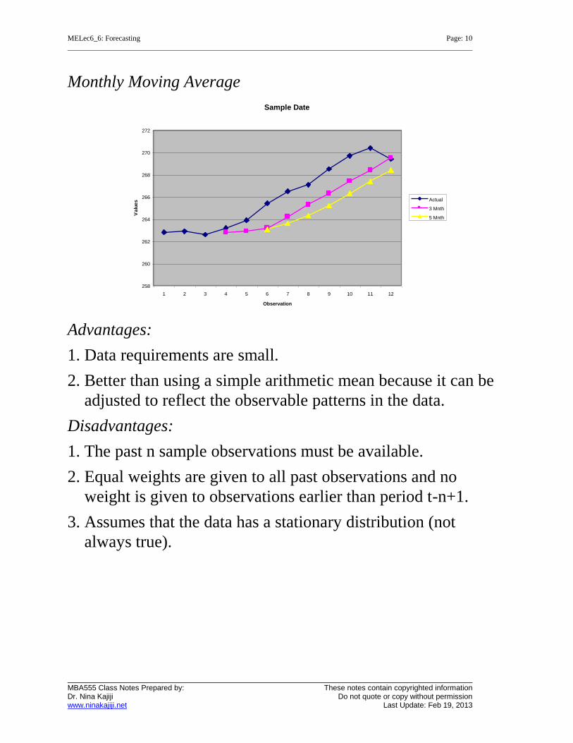
Monthly Moving Average

Sample Date

258

260

262

264

266

268

270

272

1 2 3 4 5 6 7 8 9 10 11 12

Observation

Va

lue

s Actual

3 Mnth

5 Mnth

Advantages:

1. Data requirements are small.

2. Better than using a simple arithmetic mean because it can be

adjusted to reflect the observable patterns in the data.

Disadvantages:

1. The past n sample observations must be available.

2. Equal weights are given to all past observations and no

weight is given to observations earlier than period t-n+1.

3. Assumes that the data has a stationary distribution (not

always true).



Single Exponential Smoothing

Single parameter exponential smoothing (Unadjusted) is an easy

to implement method of smoothing that overcomes some of the

problems associated with moving averages.

In contrast to moving averages, exponential smoothing permits

the researcher to weight observations. It is not unusual for

recent observations to contain more relevant information for

forecasting purposes than older ones.

The method also generates self-correcting forecasts through its

ability to produce forecast values which reflect adjustment for

earlier errors.

Advantages:

1. Simplifies forecasting calculations

2. Has small data requirements

3. Produces self-correcting forecasts with built-in adjustments

that regulate forecast values by changing them in the opposite

direction of earlier errors.

4. Simple! Only the last period’s forecast must be saved.



Disadvantages:

1. Specification of the smoothing constant is a problem. Alpha

close to 1 implies that the new forecast includes a substantial

adjustment for the error in the previous forecast. If alpha is

close to zero, the new forecast will include only a small

adjustment for error. Generally, it is suggested that if the

smoothing constant is greater than 0.30 an alternative model

should be used.

2. In general the forecasts trail the pattern in the sample data.

Notation for Single Unadjusted Exp. Smoothing

Dt := Actual value at time t

Ft+1 := Forecast value for time t+1

:= Smoothing constant

Ft+1 = Dt + (1 - )F

t-1

where: 0.0 1.0

Fo = D1 or user input.

From the above equations it is apparent that there are two

specific data input required for the unadjusted option. These

are:

1. Smoothing Constant (Alpha = ).

2. Time Series Base (D1)



Test Of Predictive Ability (Unadjusted)Time Series: B

Predicted PointSeries2

Observation

335330325320315310305300295

Actu

al &

Pre

dic

ted

138

137

136

135

134

133

132

131

130

129

128

127

126

125

124

123

122

121

120

119

118

117

116

115

114

113

112

111

110

109

Adaptive Rate of Response Single Exponential Smoothing

ARRSES

This method does not require the decision-maker to specify the

alpha smoothing constant.

ARRSES automatically changes the value of the unspecified

alpha by a predetermined weight on an on-going basis; that is,

whenever there is a change in data pattern.

The only smoothing parameter that is needed is the Beta term.

The Beta term is the weighting factor.

Advantages:

Very useful when a large number of items have to be predicted.



Disadvantages:

Unknown smoothing constant. It may not be possible to

replicate the smoothing application.

Test Of Predictive Ability (ARRSE)Time Series: B


Observation

340338336334332330328326324322320318316314312310308306304302300298

Actu

al &

Pre

dic

ted

133

132

131

130

129

128

127

126

125

124

123

122

121

120

119

118

117

116

Brown’s Linear Exponential Smoothing (Double)

Double exponential smoothing is the application of exponential

smoothing to the single exponential values.

Brown’s method provides an additional correction method; an

approach which resembles the application of a moving average.

Brown’s method uses the difference between the single and

double smoothed values as an additive factor to the single

smoothed value. The method further adjusts for the pattern in

the data.



Advantages:

Provides an additional correction for a data series - useful

when linear trend is present in the data.

Disadvantages:

The forecasts trail the pattern in the sample data.

Test Of Predictive Ability (Brown's)Time Series: B


Observation

336334332330328326324322320318316314312310308306304302300298296

Actu

al &

Pre

dic

ted

137

136

135

134

133

132

131

130

129

128

127

126

125

124

123

122

121

120

119

118

117

116

115

114

113

112

111

110

109

108

107

106



Holts’ Two Parameter Linear Exponential Smoothing

The Holt method is an extension to Brown’s method. The Holt

approach adds a growth factor to the smoothing equation. The

method smoothes the trend values directly.

When growth exists in the observed values of a time series, new

observations will be greater than the previously observed values.

Advantages:

1. Adds a growth factor to the smoothing equation.

2. Trend values are smoothed directly (unlike the implied

method in Brown)

3. Eliminates the lag in smoothing.

Disadvantages:

The forecast accuracy depends on determining the correct alpha

and beta parameters.



Test Of Predictive Ability (Holt's)Time Series: B


Observation

340338336334332330328326324322320318316314312310308306304302300

Actu

al &

Pre

dic

ted

130

129

128

127

126

125

124

123

122

121

120

119

118

117

116

115

114

113

112

111

110

109

108

107

106

105

104

103

102

101

100

99

98

97

96



Winters’ Three Parameter Model

Seasonal patterns in time series data are quite common in

business and economics. The pattern tends to occur consistently

from year to year.

Winters extended the exponential smoothing model (Holt’s

method) to incorporate seasonality factors.

Winters’ method is a three-parameter exponential smoothing

model which is used to model time series which exhibit both a

trend (Holt) and a seasonal pattern (Winters).

Advantages:

Adjusts for both the trend and the seasonality component in

the data set.

Disadvantages:

Very sensitive to the initial values for slope,

deseasonalized level, the initial seasonal factors and the

sum of the seasonal factors.



Test Of Predictive Ability (Winters')Time Series: B


Observation

340335330325320315310305300295290

Actu

al &

Pre

dic

ted

145

140

135

130

125

120

115

110

105

100

95

90

85

80

75

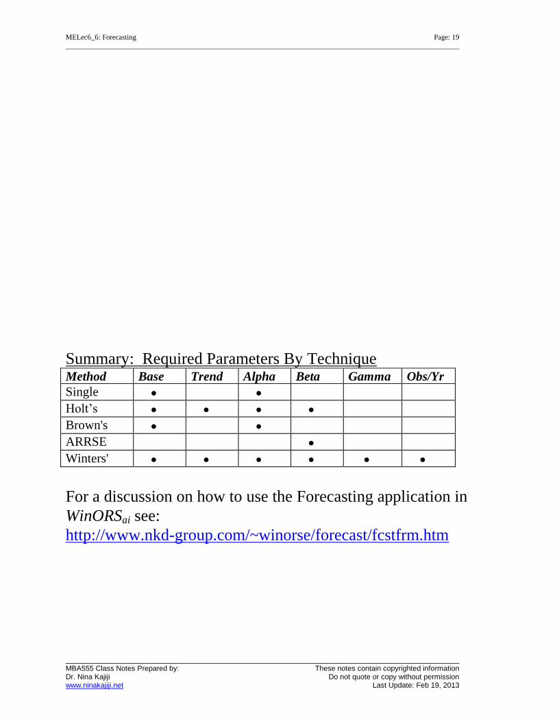
Summary: Required Parameters By Technique Method Base Trend Alpha Beta Gamma Obs/Yr

Single

Holt’s

Brown's

ARRSE

Winters'

For a discussion on how to use the Forecasting application in

WinORSai see:

http://www.nkd-group.com/~winorse/forecast/fcstfrm.htm

http://www.nkd-group.com/~winorse/forecast/fcstfrm.htm



Artificial Neural Nets (Radial Basis Function)

How do you recognize a face in a crowd? How does an

economist predict the direction of interest rates? The human

brain uses a web of interconnected processing elements called

neurons to process the information.

Each neuron is autonomous and independent. But, it also works

asynchronously (without any synchronization to other events

taking place). Neural Network algorithms rely upon the same

type of structure to solve complex problems for which you

cannot develop simple solution steps.

A neural network is a computational structure inspired by the

study of biological neural processing. Although there are many

different types of neural networks to study, we will limit our

comments to one type of neural network: the radial basis

function network (RBF).

The details of RBF are beyond the scope of our discussion. But,

we do need to know that RBF networks are used with

supervised training. By supervised, we mean that you are

required to indicate a training set of data and a test (forecast) set

of data over which the model is validated.



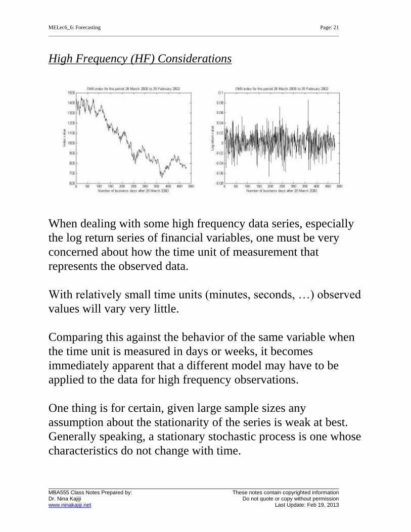
High Frequency (HF) Considerations

When dealing with some high frequency data series, especially

the log return series of financial variables, one must be very

concerned about how the time unit of measurement that

represents the observed data.

With relatively small time units (minutes, seconds, …) observed

values will vary very little.

Comparing this against the behavior of the same variable when

the time unit is measured in days or weeks, it becomes

immediately apparent that a different model may have to be

applied to the data for high frequency observations.

One thing is for certain, given large sample sizes any

assumption about the stationarity of the series is weak at best.

Generally speaking, a stationary stochastic process is one whose

characteristics do not change with time.



HF – The Leverage Effect

Changes in a commodity’s value (e.g,. stock price) tend to be

negatively correlated with changes in volatility. That is,

volatility of the time series is higher after negative shocks than

after positive shocks of the same magnitude.

HF – Long-range Dependence

In financial data it is known that the sample autocorrelations of

the data are small whereas the sample autocorrelations of the

absolute and squared values of the data are significantly

different from zero even for large lags. This behavior suggests

that there is some form of long-range dependence (memory) in

the data.

HF – Aggregational Gaussianity

In financial data, the distribution of log-returns over larger time

interval measurement (i.e., month, half year, a year) is closer to

the normal distribution than for hourly or daily (e.g., tick data)

log returns.

HF – Leptokurtic Distributions

The frequency of large and small changes, relative to the range

of the data, is somewhat high. This fact suggests that the data

do not come from a normal distribution but, rather, from a

heavy-tailed (leptokurtic) distribution. This is a distribution with

a high probability for extreme values.



HF – Volatility Clustering

Large and small values in a log return sample tend to occur in

clusters. This indicates that there is dependence in the tails.

Mandelbrot (1963): “…large changes tend to be followed by

large changes of either sign; or small changes by small

changes…”

For a discussion on how to use the ANN techniques in

WinORSai see:

RBF ANN Guide

http://www.nkd-group.com/ghdash/mba555/PDF/RBFmstr_0606.pdf



Accuracy of Forecasts

In general most forecasting methods produce forecasts that tend

to lag behind the turning points of the actual time series data.

Thus, the question arises how do you know which forecast to

recommend. There are two commonly used forecast analysis

methods in use today – Graphical Analysis and Error Measure

Analysis. When evaluating forecasts based on error measures,

the rule: smaller error value within the error measure is better

than larger error value.

Error Measures

Average Error

This is the arithmetic average of the forecast error.

Mean Percent Error (MPE %)

The mean percent error shows the error as a percentage of the

actual series. This measure is generally more informative than

average error when the original series have large differences in

their actual values.

Standard Deviation

This is the standard deviation of forecast errors.

Mean Squared Error (MSE) And Root MSE (RMSE)

This is a very common measure for evaluating the accuracy of

the forecast. The square root of this measure is also used

(RMSE).



Both MSE and RMSE tend to be overly affected by outliers.

However, it is implicitly assumed that the MSE measure is zero.

Stated differently, when the MSE is zero, then the forecasting

model is unbiased.

Mean Absolute Deviation (MAD)

MAD is less sensitive to outliers than MSE.

Other than that, it is similar in concept to MSE; the primary

difference is in its use of absolute deviations.

The use of absolute deviations is more effective if the economic

impact of forecast errors is proportional to the amount of the

errors.

Mean Absolute Percentage Error (MAPE)

MAPE is similar in concept to MAD. The major difference is

that the error terms are converted into percentage format. This

allows for direct comparison between different forecasting

methods.

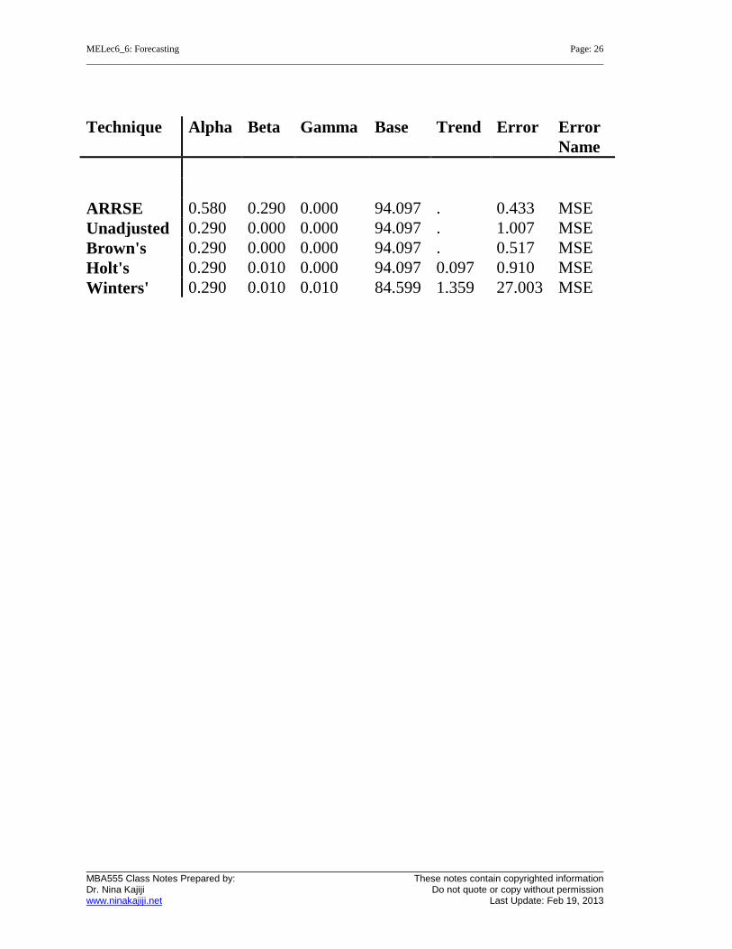
The table that follows provides a summary of the forecast

simulations for each of the methods defined above. Note that no

special attention was given to the optimization procedure. That

is and by way of example, in the case of the Winters’ technique

default simulation parameters were accepted. Hence, the

Winters’ method focused on location of an optimal Alpha

without regard to the current parameter settings for either beta

or gamma. The table is for demonstration purposes only. Each

simulation focused on location of the smallest MSE as a

measurement of forecast error.



Technique Alpha Beta Gamma Base Trend Error Error

Name

ARRSE 0.580 0.290 0.000 94.097 . 0.433 MSE

Unadjusted 0.290 0.000 0.000 94.097 . 1.007 MSE

Brown's 0.290 0.000 0.000 94.097 . 0.517 MSE

Holt's 0.290 0.010 0.000 94.097 0.097 0.910 MSE

Winters' 0.290 0.010 0.010 84.599 1.359 27.003 MSE



Graphical Analysis

After each execution of the forecasting method, the actual,

predicted and residual terms can be compared graphically.

Graphical analysis is used to augment the interpretation of the

forecast. Overall quality of fit can be judged from the graphical

analysis.

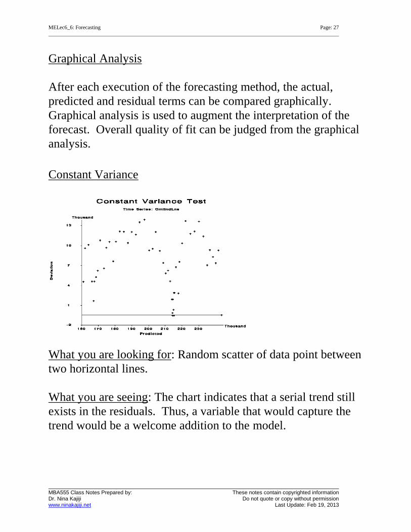
Constant Variance

What you are looking for: Random scatter of data point between

two horizontal lines.

What you are seeing: The chart indicates that a serial trend still

exists in the residuals. Thus, a variable that would capture the

trend would be a welcome addition to the model.



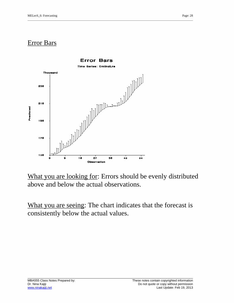
Error Bars

What you are looking for: Errors should be evenly distributed

above and below the actual observations.

What you are seeing: The chart indicates that the forecast is

consistently below the actual values.



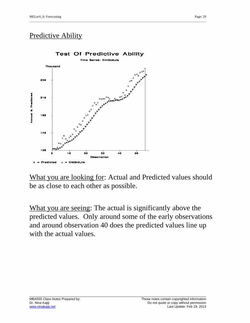
Predictive Ability

What you are looking for: Actual and Predicted values should

be as close to each other as possible.

What you are seeing: The actual is significantly above the

predicted values. Only around some of the early observations

and around observation 40 does the predicted values line up

with the actual values.



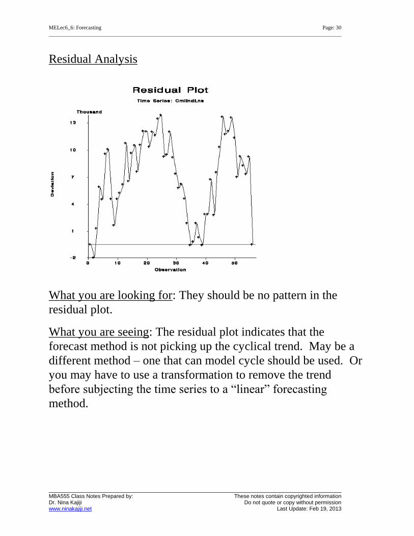
Residual Analysis

What you are looking for: They should be no pattern in the

residual plot.

What you are seeing: The residual plot indicates that the

forecast method is not picking up the cyclical trend. May be a

different method – one that can model cycle should be used. Or

you may have to use a transformation to remove the trend

before subjecting the time series to a “linear” forecasting

method.



How to Communicate Forecasts

1. Purpose or usefulness of the forecast (including its time

frame)

2. Key underlying assumptions

3. Input data

4. Forecast values

5. Graphic display of history with predictions

6. Any other comments or stipulations that are needed to

place the forecast in proper perspective – include a

discussion on the error measure to support your forecast.

7. Reporting on the past forecasting performance record – if

possible.

Date post:	04-Jun-2018
Category:	Documents
Upload:	vuongnguyet
View:	217 times
Download:	0 times

ADVANCED BUSINESS FORECASTING - NKD Group · Exponential smoothing family ... Seasonal Variation...

Documents