1

Advanced Cement-Based Sustainable Material Technology

Zongjin LiHong Kong University of Science and Technology

2

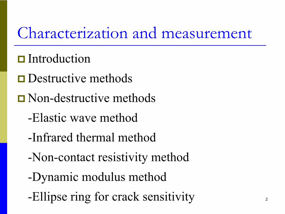
Characterization and measurementIntroductionDestructive methodsNon-destructive methods-Elastic wave method-Infrared thermal method-Non-contact resistivity method-Dynamic modulus method-Ellipse ring for crack sensitivity

3

IntroductionDestructive test – obtain the

material properties by seriously destroying sample

Nondestructive test – obtain the information without damaging samples

4

Introduction-destructive methodsCompression testTension testBending testImpact test

5

Introduction-nondestructiveQuality control

Finished productsInjection of groutPosition of reinforcing steelWelding of reinforcing steelHydration rate of fresh concreteSelection of watermelon and eggs

6

Introduction-nondestructiveb. In-service inspection

Boiler and vesile safety monitoringBridge safety monitoringBuilding finish monitoringAirplane

7

Destructive tests -

Control methods for strength test

Open Loop Control (OLC)Close Loop Control (CLC)

Input variable(Reference Input)

Prescribed functionController Controlled Process

Output variable

Measured Output

Input variable(Reference Input)

Prescribed functionController Controlled Process

Output variable

Measured OutputFeedback Signal

Open Loop Control (OLC)

Closed Loop Control (CLC)

8

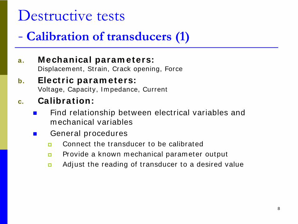
Destructive tests -

Calibration of transducers (1)

a. Mechanical parameters: Displacement, Strain, Crack opening, Force

b. Electric parameters: Voltage, Capacity, Impedance, Current

c. Calibration:Find relationship between electrical variables and mechanical variablesGeneral procedures

Connect the transducer to be calibratedProvide a known mechanical parameter outputAdjust the reading of transducer to a desired value

9

c. Calibratione.g. A displacement transducer of 2.5mm full range

Destructive tests -

Calibration of transducers (2)

Displacement:

Voltage:

0.25

. . . .

0.5

. . . .

1.25

. . . .

2.5mm

1 . . . .

2

. . . .

5

. . . .

10V

V

D (mm)

k

10

2.5

For measurement:

Displacement = = C V

10

Destructive tests -

Calibration of transducers (3)

Transducer

11

Destructive tests-

Compressive test (1)

A set-up for compression test

12

Destructive tests-

Compressive test (2)

Typical load versus axial displacement and load versus circumferential Displacement curves for three classes for concrete

13

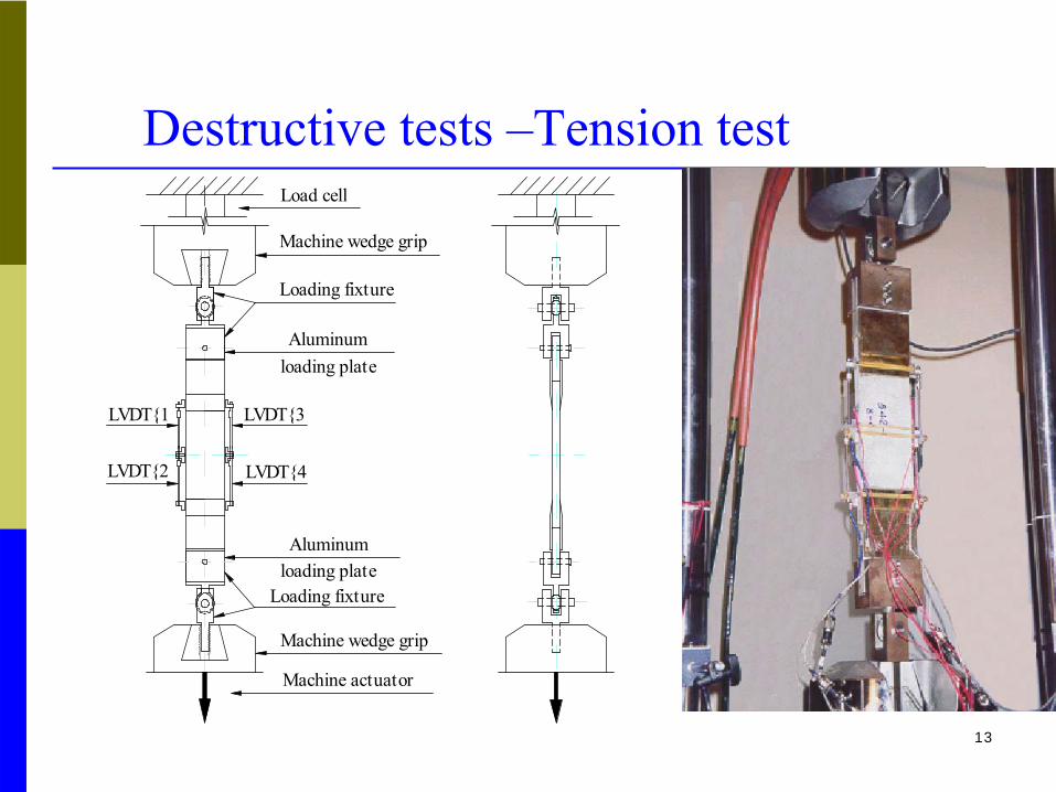
Load cell

Machine wedge grip

Loading fixture

Aluminum

LVDT{1 LVDT{3

loading plate

LVDT{4

Aluminumloading plate

LVDT{2

Loading fixture

Machine wedge grip

Machine actuator

Destructive tests –Tension test

14

0.00 0.02 0.04 0.06 0.08 0.10

Displacement (mm)

0

1

2

3

4

5

Steel fiber (0.5% in volume)

Polypropylene fiber (0.5% in volume)

Plain concrete

Destructive tests –Tension test

15

Nondestructive test -Shear wave reflection method

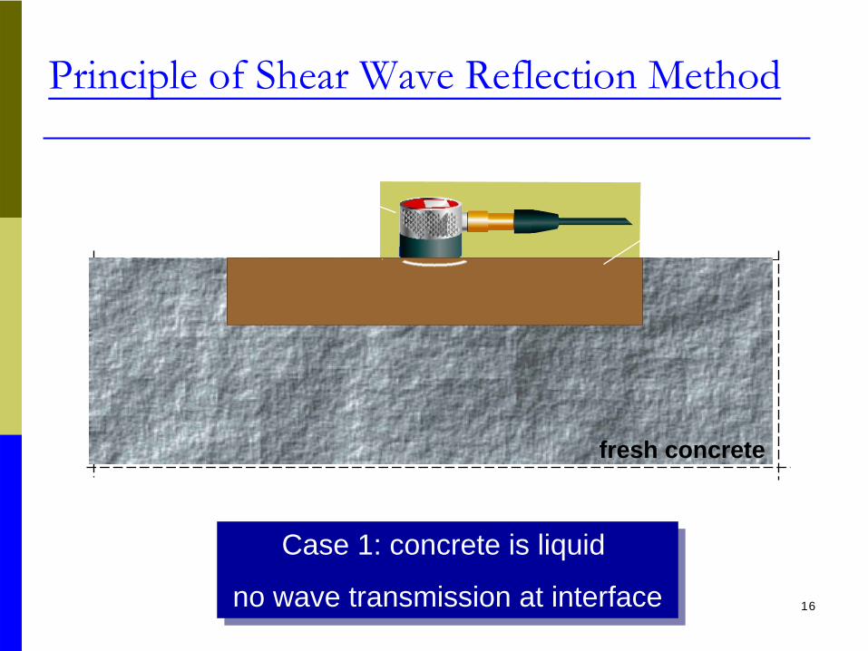
16shear waves: do not propagate in liquids

Case 1: concrete is liquid

no wave transmission at interface

Case 1: concrete is liquid

no wave transmission at interface

fresh concrete

steel plateshear wave transducer (2.25 MHz)

Principle of Shear Wave Reflection Method

17

Principle of Wave Reflection

fresh Concrete

Case 2: concrete is hardening

transmission losses at interface

Case 2: concrete is hardening

transmission losses at interface

hardened concrete

steel plateshear wave transducer (2.25 MHz)

18

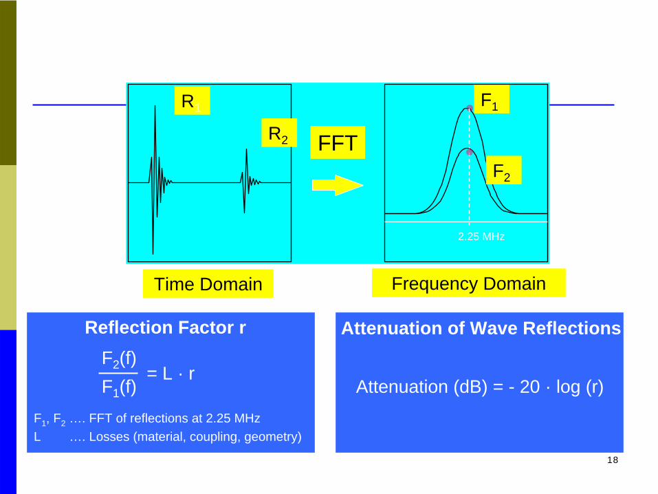
Signal Analysis

Reflection Factor r

F1 , F2 …. FFT of reflections at 2.25 MHzL …. Losses (material, coupling, geometry)

F2 (f)F1 (f)

= L · r

Attenuation of Wave Reflections

Attenuation (dB) = - 20 · log (r)

Time Domain Frequency Domain

R1

R2

F2

F1

FFT

2.25 MHz

19

Typical Reflection Loss Development

Phase 1: liquid concrete no reflection loss

Phase 2: concrete hardens attenuation increases

Phase 3: hardening continues attenuation approaches final value

Ref

lect

ion

Loss

Phase 1 Phase 2

Point A

Phase 3

Point B

20

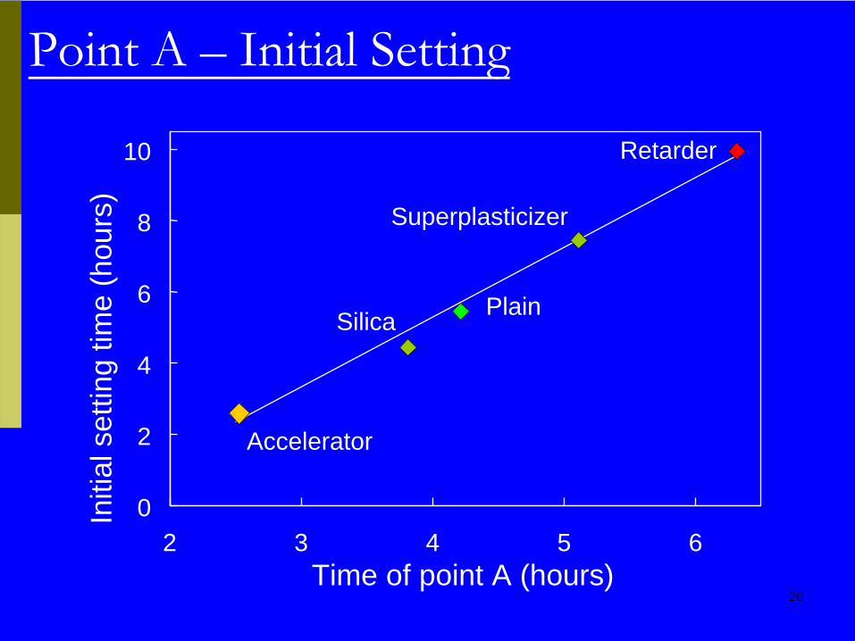
Point A – Initial Setting

0

2

4

6

8

10

2 3 4 5 6Time of point A (hours)

Initi

al s

ettin

g tim

e (h

ours

)

PlainSilica

Superplasticizer

Accelerator

Retarder

21

0

10

20

30

40

50

0 1 2 3 4

RL

vs. Strength

w/c = 0.35w/c = 0.6

w/c = 0.5

R2 = 0.97

R2 = 0.92 Transition Pointbetween 6 – 15 hours

Cement Mortarsdifferent w/c-ratios

Com

pres

sive

Stre

ngth

(MP

a)

Reflection Loss (dB)

22Transducer Central Power Supply

Main Power Switch

Laptop Computer

Pulser/ Receiver

Temperature Logger

23

Steel Plates

On-Site Measurements

24

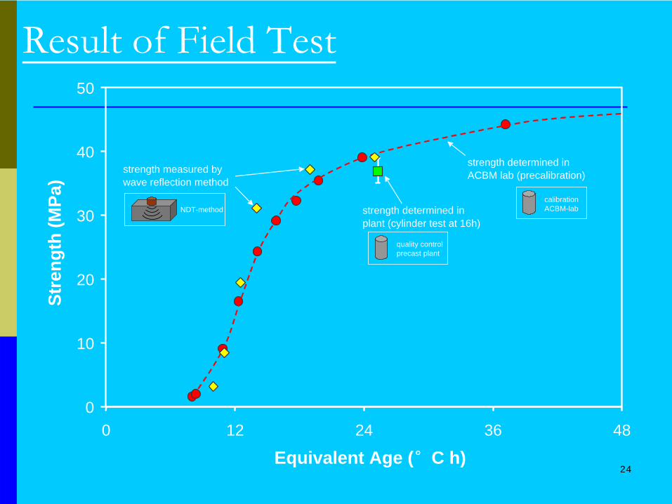
Result of Field Test

0

10

20

30

40

50

0 12 24 36 48

Equivalent Age (°C h)

Stre

ngth

(MPa

)

strength determined in ACBM lab (precalibration)

strength determined in plant (cylinder test at 16h)

quality controlprecast plant

calibrationACBM-lab

strength measured by wave reflection method

NDT-method

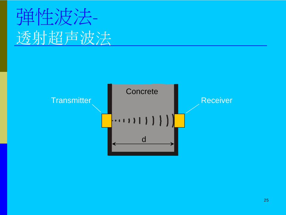
25

弹性波法- 透射超声波法

d

ConcreteTransmitter Receiver

26

Pulse VelocityDetermination

Amplitude Threshold

to – Onset time of signal

AT

TimeAm

plitu

de

Relationships

( )( )( )2ν1ν1ρ

ν1EvP −+−

=

( )ν12ρEvS +

=

P-waves

S-waves

Velocity ~Density, ρE-Modul, EPoisson's Ratio, ν

Time Domain

d

tdvΔ

=

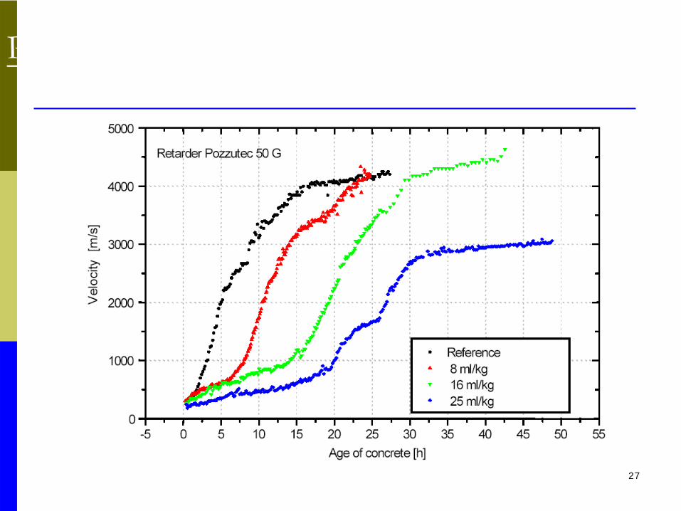
27

Pulse Velocity Measurements

from Reinhardt, Grosse, University of Stuttgart

Sensitivity to hydration rate influenced by retarder

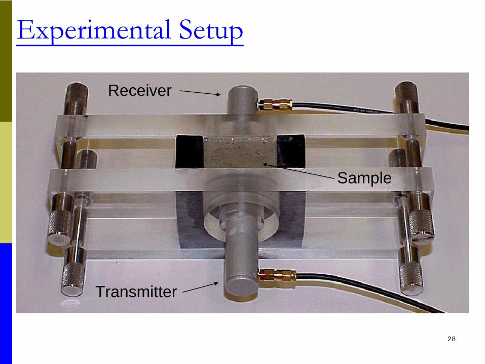
28

Experimental Setup

Transmitter

Receiver

Sample

29

Embedded sensor

Function generator

Poweramplifier

Pre-

amplifier

Oscilloscope

Transmitter Receiver

30

31

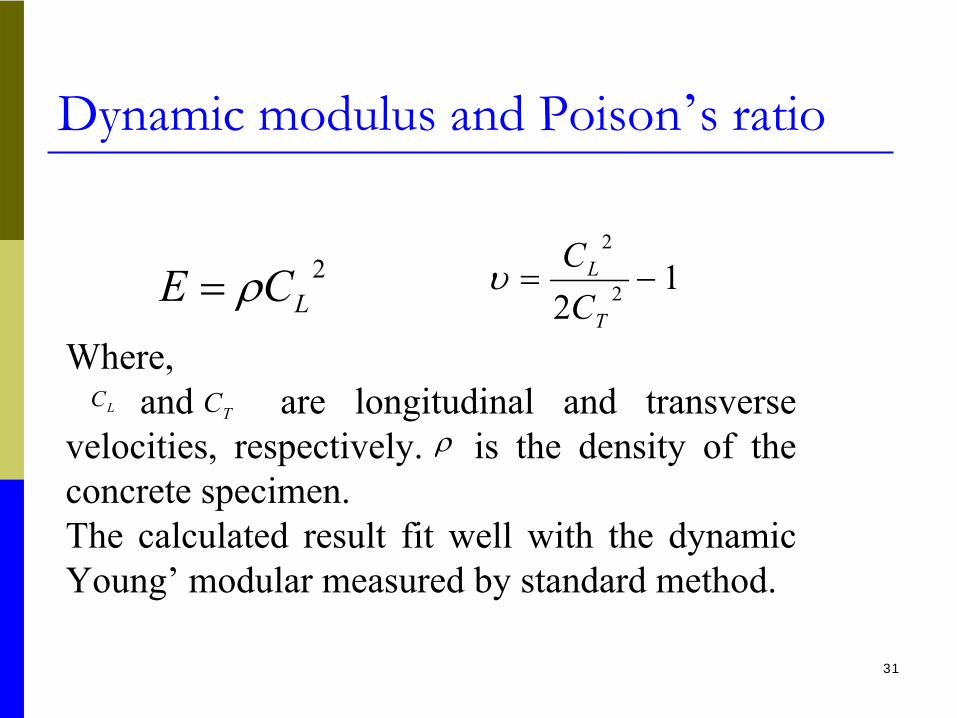
Dynamic modulus and Poison’s ratio

2LCE ρ= 1

2 2

2

−=T

L

CCυ

Where,and are longitudinal and transverse

velocities, respectively. is the density of the concrete specimen.The calculated result fit well with the dynamic Young’

modular measured by standard method.

LCTC

ρ

32

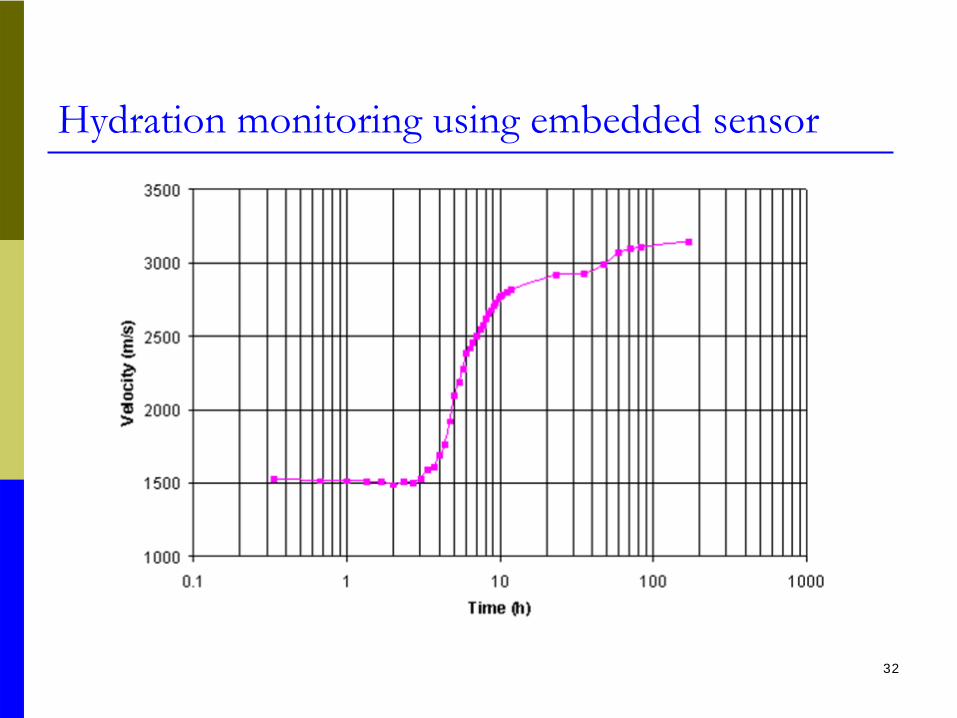
Hydration monitoring using embedded sensor

33

Hydration monitoring using embedded sensor

传感器埋置

监测中33

In situ and real time monitoring

Life time healthy monitoring

34

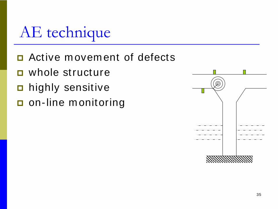
AE techniqueAE technique is a passive NDT method. It relies on the detection of elastic waves generated by sudden release or change of energy or deformation in materials.

35

AE techniqueActive movement of defectswhole structure highly sensitiveon-line monitoring

36

聲發射測試技術

AE Transducer

AE Transducer

A acoustic wave propagation

37

Basic AE measurement system

38

AE technique

39

AE Technique

Occurrence of AE rate during the tension test

40

AE technique

41

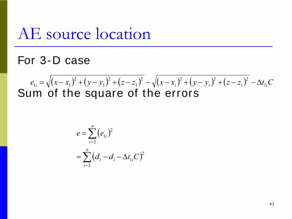
AE source location For 3-D case

Sum of the square of the errors( ) ( ) ( ) ( ) ( ) ( ) Ctzzyyxxzzyyxxe iiiii 1

22221

21

211 Δ−−+−+−−−+−+−=

( )

( )∑

∑

=

=

Δ−−=

=

n

iii

n

ii

Ctdd

ee

2

211

2

21

42

AE source locationDifferential with respect to x, y, z and C are in forms of;

( )

( )iCΔtddd

xxd

xxxeCx,y,zf

i

n

i i

i

x

112 1

12

,

−−⎟⎟⎠

⎞⎜⎜⎝

⎛ −−

−=

∂∂

=

∑=

( )

( )iCΔtddd

yyd

yyyeCx,y,zf

i

n

i i

i

y

112 1

12

,

−−⎟⎟⎠

⎞⎜⎜⎝

⎛ −−

−=

∂∂

=

∑=

43

AE source location

( )

( )iCΔtddd

zzd

zzzeCx,y,zf

i

n

i i

i

z

112 1

12

,

−−⎟⎟⎠

⎞⎜⎜⎝

⎛ −−

−=

∂∂

=

∑=

( )

( )∑=

−+ΔΔ=∂∂

=n

iiii

C

ddCttCeCzyxf

21112

,,,

44

AE source location

AE events during period between pre 0.0 to 0.8 peak load

45

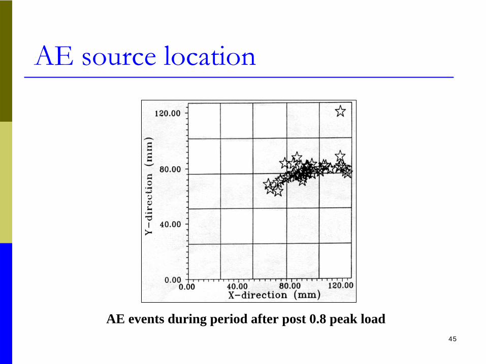
AE source location

AE events during period after post 0.8 peak load

46

AE source location

AE events during period between pre 0.0 to post 0.8 peak load

47

AE source location

Major crack position for concrete specimen C-M13

48

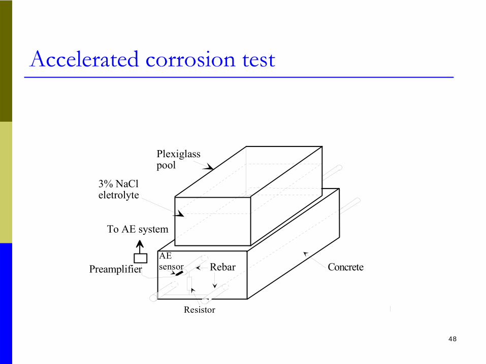
Accelerated corrosion test

Concrete

3% NaCleletrolyte

Plexiglasspool

Rebar

To AE system

AEsensorPreamplifier

Resistor

49

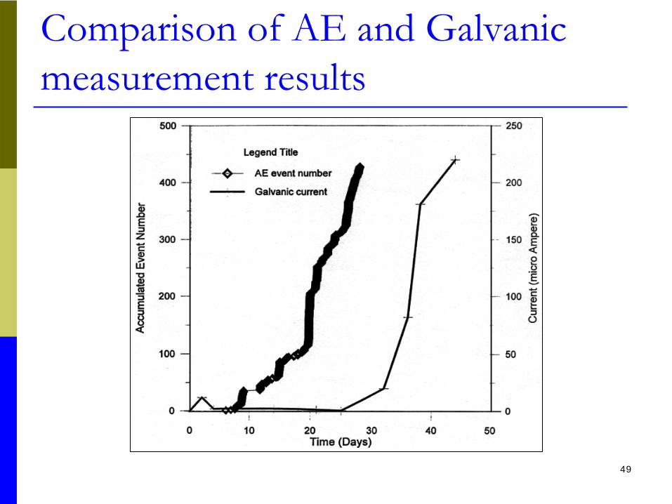
Comparison of AE and Galvanic measurement results

50

51

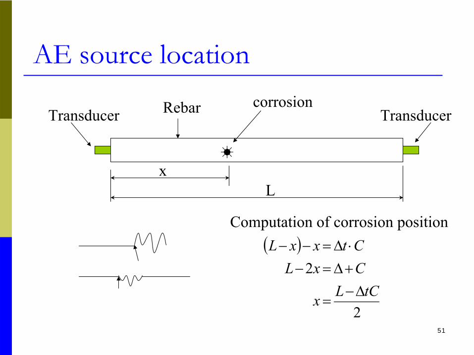
AE source location

Computation of corrosion position

Lx

Transducer TransducerRebar corrosion

( )

2

2tCLx

CxLCtxxL

Δ−=

+Δ=−⋅Δ=−−

52

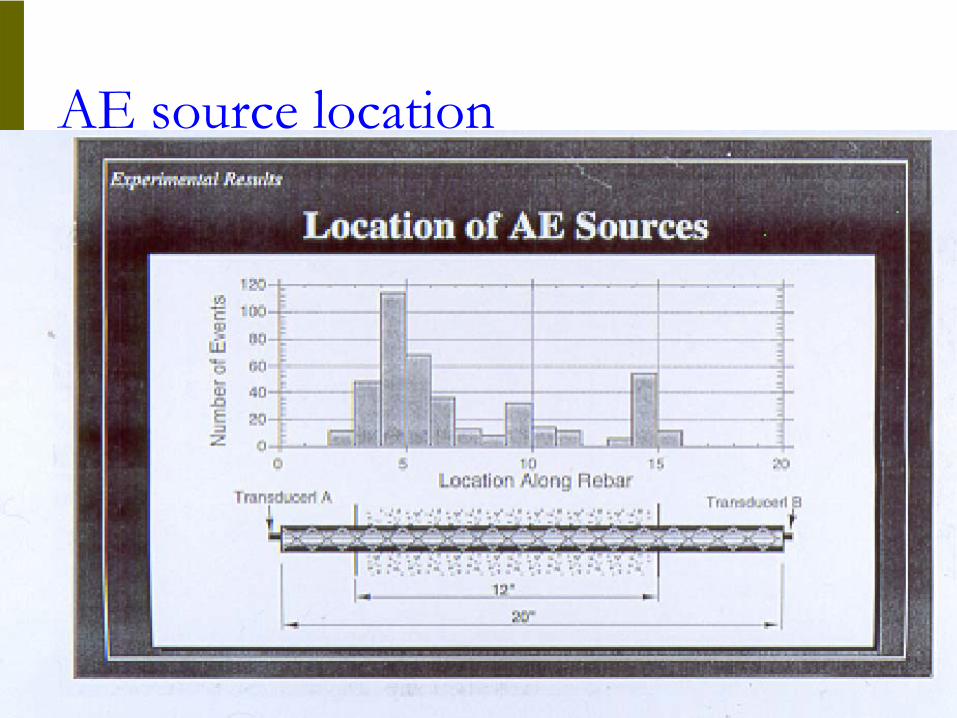
AE source location

53

AE source location

54

Infrared thermograph --Introduction (1)

a) LightAn electromagnetic wave and travels at

3x108 m/s

EM waves can be either visible or invisible according to their wavelength

55

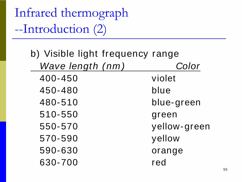
Infrared thermograph --Introduction (2)

b) Visible light frequency rangeWave length (nm) Color400-450 violet450-480 blue480-510 blue-green510-550 green550-570 yellow-green570-590 yellow590-630 orange630-700 red

56

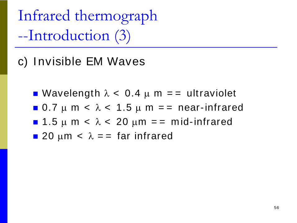
Infrared thermograph --Introduction (3)

c) Invisible EM Waves

Wavelength λ < 0.4 μ m == ultraviolet0.7 μ m < λ < 1.5 μ m == near-infrared1.5 μ m < λ < 20 μm == mid-infrared20 μm < λ == far infrared

57

Infrared thermograph --Introduction (4)

d) Infrared frequency range

58

Infrared thermograph --Mechanism (1)

Emission of EM waves by objects(The principle of blackbody radiation)Any object at non-zero temperature emits

EM waves

59

Infrared thermograph --Mechanism (2)

Infrared radiation and temperature relatedThe wavelength of ITC is within the emission wavelength range of any object in the normal temperature range of -30oC to 100oC.Defects underneath can be detected by measuring the slight temperature fluctuation over the surface of an object.

60

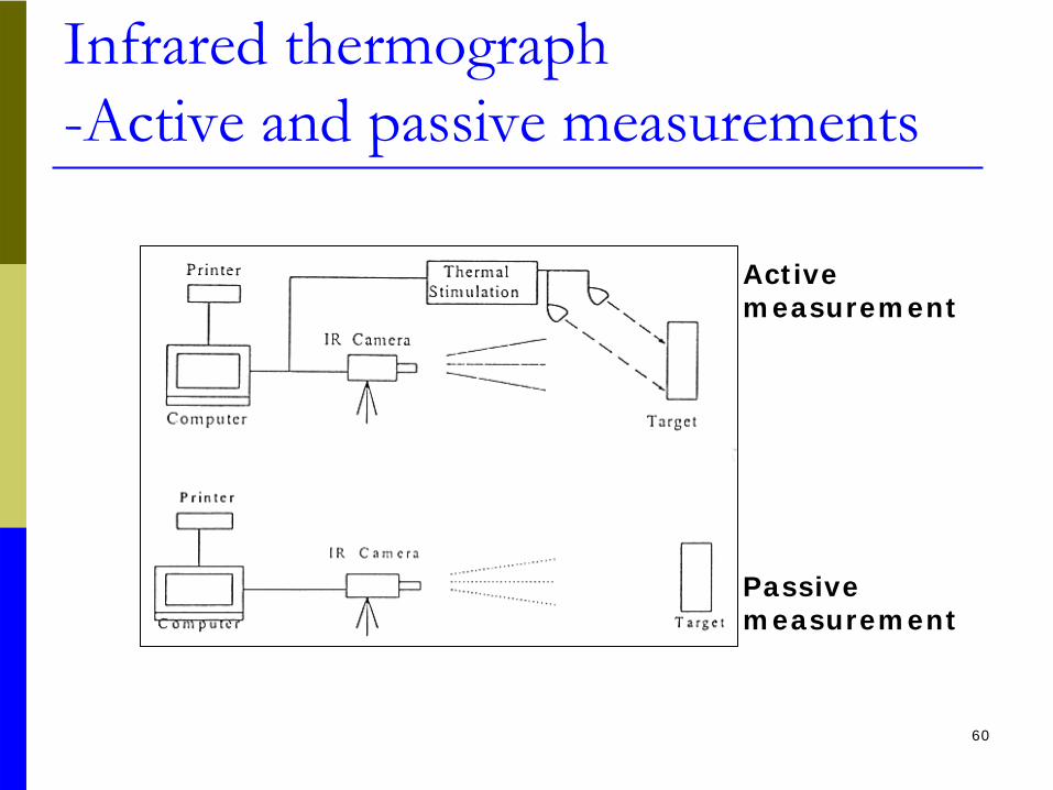
Infrared thermograph -Active and passive measurements

Active measurement

Passive measurement

61

Theoretical background for debonded tile detection (1)

B - Heat capacitanceH - Heat flow rateK - Thermal conductivity

Initial condition:t=0, T=T0

)( 0TTKHdtdTB −−=

62

Theoretical background for debonded tile detection (2)

For heating process (H>0)

For cooling process (H<0)

⎟⎟⎠

⎞⎜⎜⎝

⎛−+=

− tBK

eKHTT 10

⎟⎟⎠

⎞⎜⎜⎝

⎛−−=

− tBK

eKH

TT 10

63

Two Cases (1)Two cases for voids between tile and

substrateCase 1 = = voids are filled with waterCase 2 = = Voids are empty (filled with air)

64

Two Cases (2)

Heat Capacity(J cm-3

C-1)

Conductivity(W m-1

C-1)Material

Air

Concrete

Water

0.0008

1.9

4.2

0.024

1

0.6

Thermal Properties

65

Two Cases (3)Case 1: Gap filled with water

During Heating proces

H/K K/BConcrete H ~1/1.9≈0.5Water 1.6H ~1/7 ≈0.14∴T is lower than concreteDuring Cooling processT is higher than concrete

⎟⎟⎠

⎞⎜⎜⎝

⎛−+=

− tBK

eKHTT 10

66

Two Cases (4)Case 2: Gap filled with air

During Heating proces

H/K K/BConcrete H ~0.5Water 42H ~30∴T is higher than concreteDuring Cooling processT is lower than concrete

⎟⎟⎠

⎞⎜⎜⎝

⎛−+=

− tBK

eKHTT 10

67

Two Cases (5)

A debonded tile sample with half air and half wateruniform heating of the inspected faceafter cooling for half an hour.

68

Examples (1)

Thermal image of HKUST library indicating defected area

filled with water on the external tiled wall

69

Examples (2)

Thermograph of the government staff quarter under

sunshine - indicating heavy damage on external wall

70

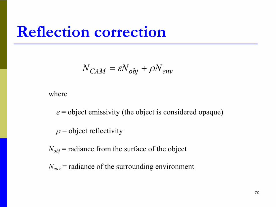
Reflection correction

where

ε = object emissivity (the object is considered opaque)

ρ = object reflectivity

Nobj = radiance from the surface of the object

Nenv = radiance of the surrounding environment

envobjCAM NNN ρε +=

71

Reflection correctionHigh emissivity case (ε > 0.9. ε = (1-ρ))

Nobj ≈

NCAM

Low emissivity case (ε < 0.9)Reflection should be considered

Ceramic tile case (ε = 0.6 - 0.8)Reflection can not be neglected

72

Reflection correction

……

Image 1

Image 2

Image n

Time

73

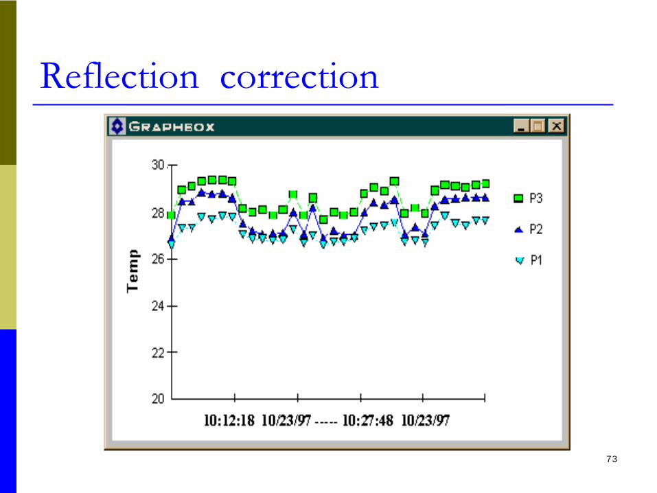
Reflection correction

74

Distance and angle --Space resolutionField view of an ITC depends on the lens of the systemA camera may consist of 320 x 240 detectors in an arrayThe area covered by each detector is the smallest size of an object Instantaneous field of view (IFOV)

75

Distance and angle - Space resolutionExample (20 degree by 15 degree lens)

Distance to object Field of view IFOV

1m 0.35 x 0.26 m 1.1 x 1.1mm

5m 1.76 x 1.32 m 5.5 x 5.5mm

10m 3.52 x 2.63 m 11 x 11mm

50m 17.6 x 13.2 m 55 x 55mm

76

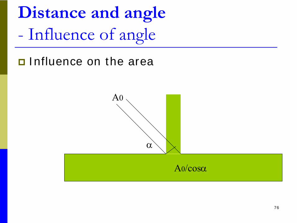
Distance and angle - Influence of angleInfluence on the area

A0/cosα

A0

α

77

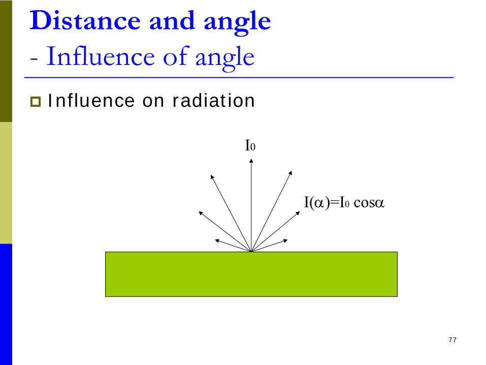
Distance and angle - Influence of angleInfluence on radiation

I0

I(α)=I0

cosα

78

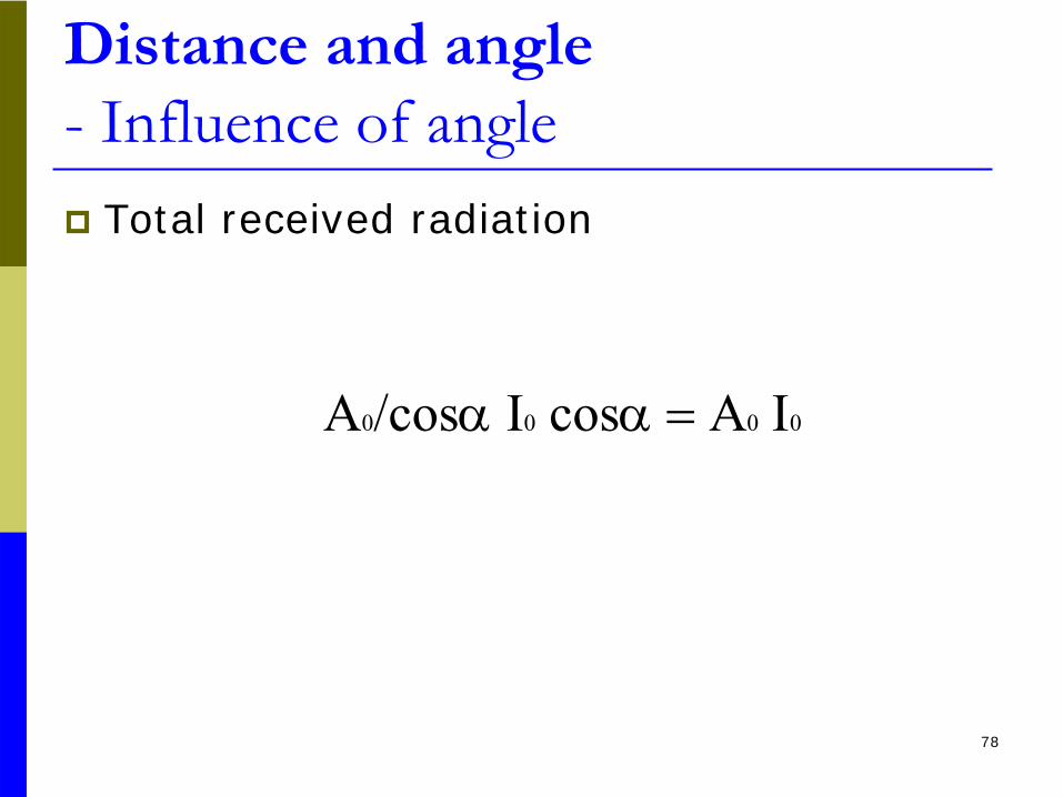
Distance and angle - Influence of angleTotal received radiation

A0

/cosα

I0

cosα = Α0

Ι0

79

Distance and angle - Influence of angleThumb rule for reality - No [erfectly diffuse bodies exist- For most bodies, the emissivity uually goes down from 50 degree from normal

80

Cement conduction mechanism

cationanion

anodecathode

Conduction in cement is essentially electrolytic via ion transport through the interconnected pore network.

Resistivity

81

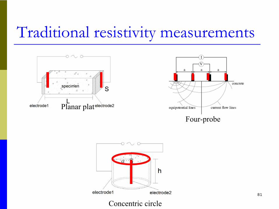
Traditional resistivity measurements

Planar plat

Concentric circle

Four-probe

82

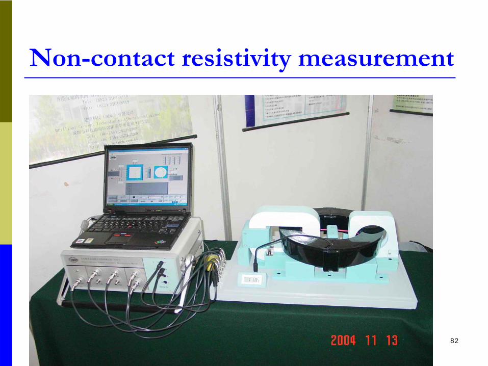
Non-contact resistivity measurement

83

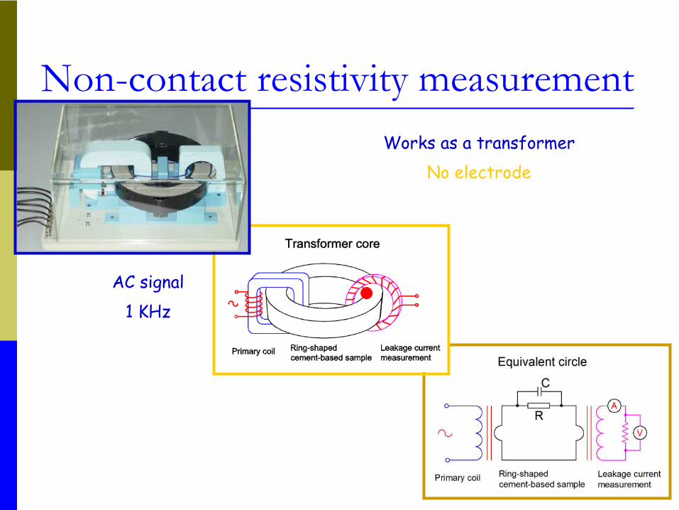
Non-contact resistivity measurementWorks as a transformer

No electrode

AC signal1 KHz

84

ρ= Rtotal π2h[ ln(r3/r2) +

34

4

rrr−

ln(r4/r3) -12

1

rrr−

ln(r2/r1)]

Analytical solution of resistivity

85

ProceduresWeighing and mixing

water and cement at

w/c=0.3, 0.35, 0.4 for 4 minutesConsequently, casting

into electrical

resistivity mouldRecording

the data at sampling interval 1

minute and stop at or after 24 hoursMeasuring

the weight and height of the

sampleAnalyzing

in EXCEL and smooth/

differential in Origin to get dρ/dt

curve and get the maximum dρ/dt

point

86

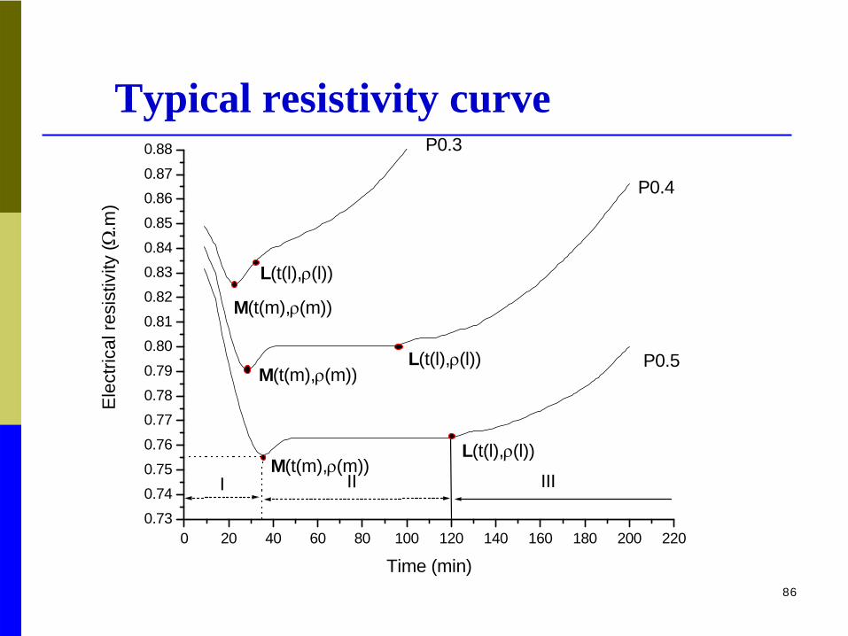
0 20 40 60 80 100 120 140 160 180 200 2200.730.740.750.760.770.780.790.800.810.820.830.840.850.860.870.88

L(t(l),ρ(l))

L(t(l),ρ(l))

L(t(l),ρ(l))

IIIM(t(m),ρ(m))

M(t(m),ρ(m))

M(t(m),ρ(m))

III

P0.5

P0.4

P0.3

Ele

ctric

al re

sist

ivity

(Ω.m

)

Time (min)

Typical resistivity curve

87

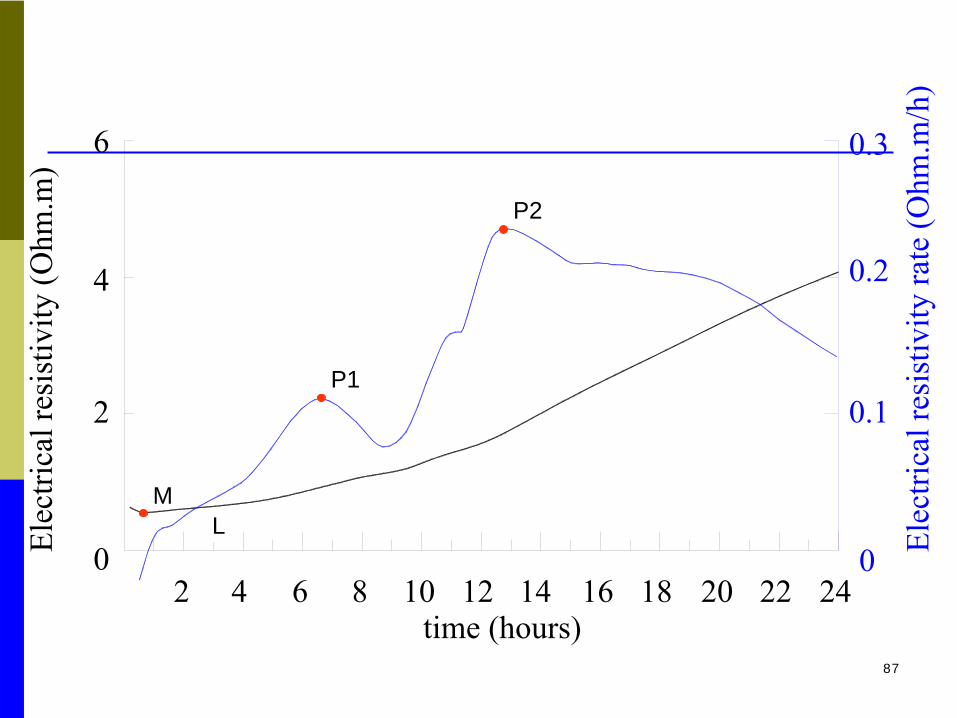
18

6

Elec

trica

l res

istiv

ity (O

hm.m

)

02 4 6

2

4

time (hours)128 10 14 16

Elec

trica

l res

istiv

ity ra

te (O

hm.m

/h)

0.3

2420 220

0.1

0.2

M

P1

P2

L

88

18

6

Elec

trica

l res

istiv

ity (O

hm.m

)

02 4 6

2

4

time (hours)128 10 14 16

Elec

trica

l res

istiv

ity ra

te (O

hm.m

/h)

0.3

2420 220

0.1

0.2

M

P1

P2

Dyna. bala. Setting Hardening Hardening decelerationDissolution

L

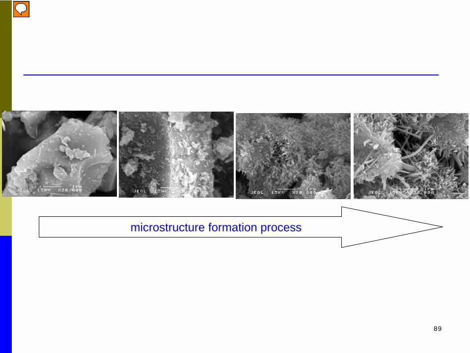
89

microstructure formation process

90

Penetration method for setting time

Initial setting:Penetration resistance:

3.5 MPa

Final setting:Penetration resistance:

28

MPa

(ASTM 403)

91

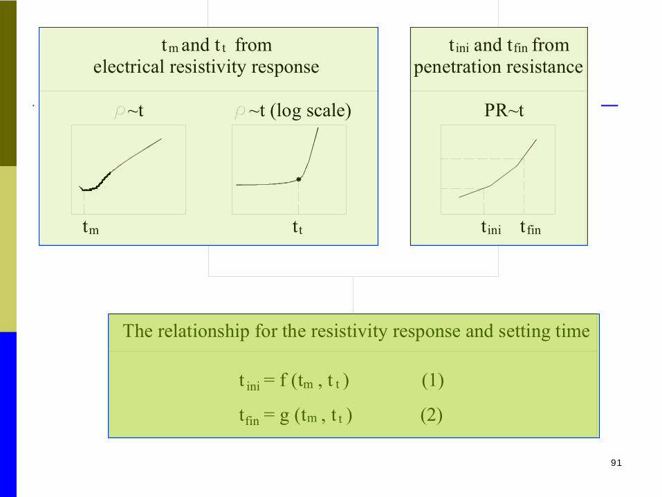
t = g (t , t ) (2)

t = f (t , t ) (1)

The relationship for the resistivity response and setting time

~t (log scale)

tm

fin

ini

m

m

t

t

tt

electrical resistivity response

~t

t and t fromm t

init tfin

t and t frompenetration resistance

PR~t

ini fin

92

93

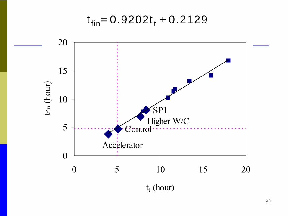
tfin =0.9202tt +0.2129

Accelerator

SP1

ControlHigher W/C

0

5

10

15

20

0 5 10 15 20

tt (hour)

t fin (

hour

)

94

t = g (t , t ) (2)

t = f (t , t ) (1)

The relationship for the resistivity response and setting time

~t (log scale)

tm

fin

ini

m

m

t

t

tt

electrical resistivity response

~t

t and t fromm t

init tfin

t and t frompenetration resistance

PR~t

ini fin

95

0

5

10

15

20

0 2 4 6 8 10 12 14 16 18

Measured tini and tfin (hours)

Cal

cula

ted

t ini a

nd t

fin (

hour

s)

tini

tfin

96

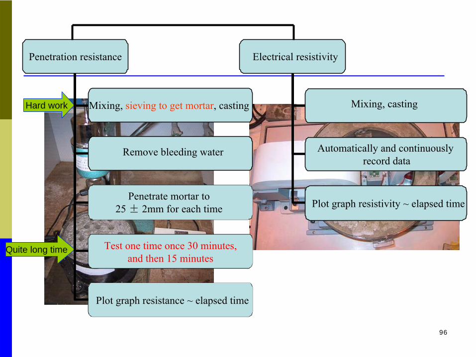
Mixing, sieving to get mortar, casting

Remove bleeding water

Penetrate mortar to25 ± 2mm for each time

Test one time once 30 minutes, and then 15 minutes

Plot graph resistance ~ elapsed time

Mixing, casting

Automatically and continuously record data

Plot graph resistivity ~ elapsed time

Hard work

Quite long time

Penetration resistance Electrical resistivity

97

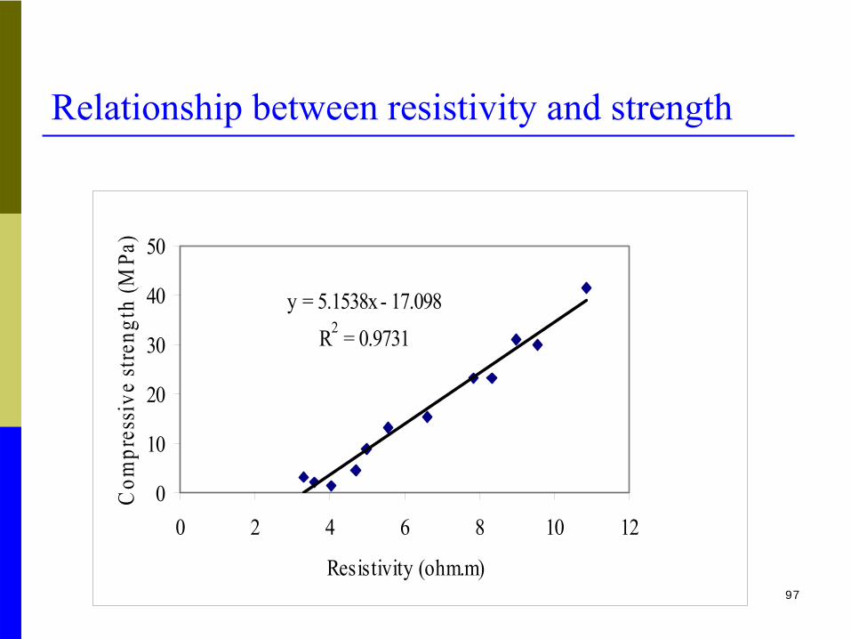
Relationship between resistivity and strength

y = 5.1538x - 17.098R2 = 0.9731

0

10

20

30

40

50

0 2 4 6 8 10 12

Resistivity (ohm.m)

Com

pres

sive

stre

ngth

(MPa

)

98

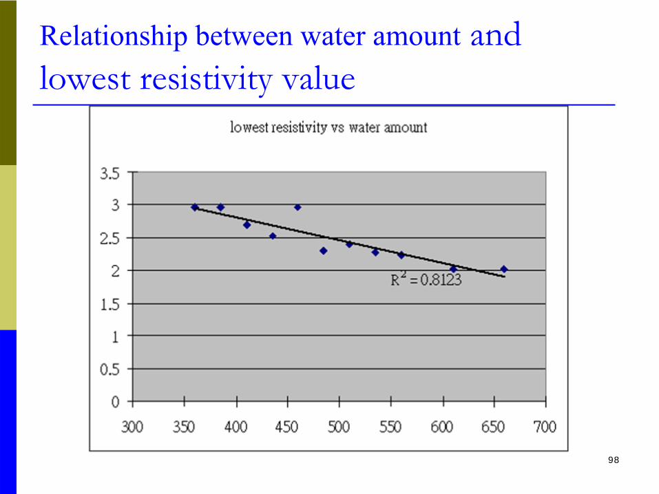
Relationship between water amount

and lowest resistivity value

99

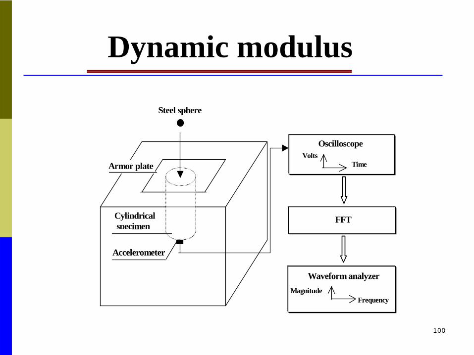
Dynamic modulus

Induce an impact

Accelerator receive the vibration response and transfer them to the Data Acquisition Unit

Frequency display on the Signal Analysis Unit

100

Accelerometer

Cylindrical specimen

Steel sphere

Armor plate

OscilloscopeVolts

Time

FFT

Waveform analyzer

FrequencyMagnitude

Dynamic modulus

101

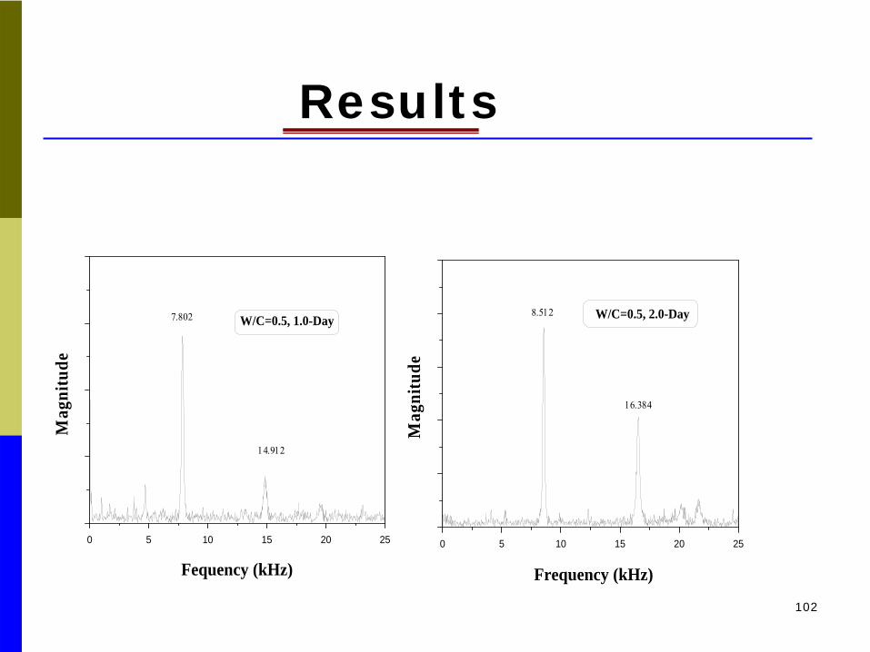
Results

0 5 10 15 20 25

4.704

8.992

Frequency (kHz)

Mag

nitu

de

W/C=0.5 8.0 Hours

0 5 10 15 20 25

5.408

10.34

Frequency (kHz)

Mag

nitu

de

W/C=0.5, 0.5-Day

102

0 5 10 15 20 25

7.802

14.912

Mag

nitu

de

Fequency (kHz)

W/C=0.5, 1.0-Day

0 5 10 15 20 25

8.512

16.384

Frequency (kHz)

Mag

nitu

de

W/C=0.5, 2.0-Day

Results

103

0 5 10 15 20 25

8.832

16.896

W/C=0.5, 3.0Day

Mag

nitu

de

Frequency (kHz)0 5 10 15 20 25

10.048 kHz

19.296 kHz

W/C=0.5, 28.0-Day

Mag

nitu

de

Frequency (kHz)

Results

104

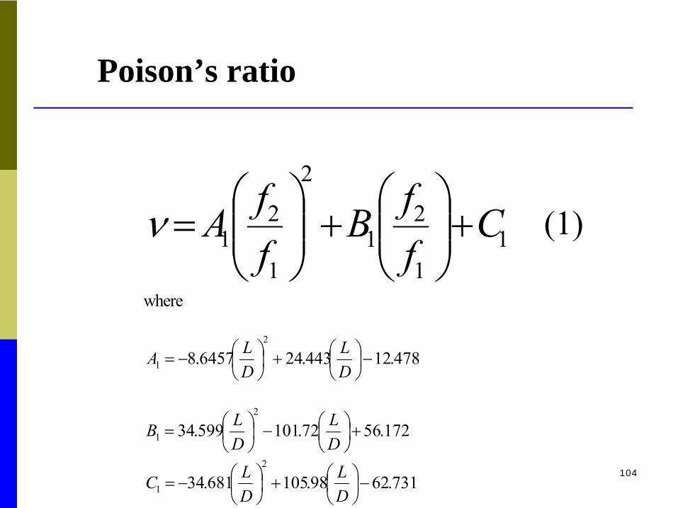
11

21

2

1

21 C

ffB

ffA +⎟⎟

⎠

⎞⎜⎜⎝

⎛+⎟⎟

⎠

⎞⎜⎜⎝

⎛=ν

where

478.12443.246457.82

1 −⎟⎠⎞

⎜⎝⎛+⎟

⎠⎞

⎜⎝⎛−=

DL

DLA

172.5672.101599.342

1 +⎟⎠⎞

⎜⎝⎛−⎟

⎠⎞

⎜⎝⎛=

DL

DLB

731.6298.105681.342

1 −⎟⎠⎞

⎜⎝⎛+⎟

⎠⎞

⎜⎝⎛−=

DL

DLC

(1)

Poison’s ratio

105

0 4 8 12 16 20 24 280.00

0.05

0.10

0.15

0.20

0.25

0.30

W/C = 0.5, Plain Concrete

W/C = 0.6, Plain ConcretePois

son'

s rat

io

Age (Days)

Poison’s ratio

106

( )2

101 212 ⎟⎟

⎠

⎞⎜⎜⎝

⎛+=

nd f

RfE πρν

where

( ) ( ) 222

21 CBAfn ++= νν 3791.15868.00846.0

2

2 +⎟⎠⎞

⎜⎝⎛−⎟

⎠⎞

⎜⎝⎛=

DL

DLB

1093.24585.12792.02

2 −⎟⎠⎞

⎜⎝⎛+⎟

⎠⎞

⎜⎝⎛−=

DL

DLA 3769.37026.1285.0

2

2 +⎟⎠⎞

⎜⎝⎛−⎟

⎠⎞

⎜⎝⎛=

DL

DLC

(2)

Dynamic modulus

107

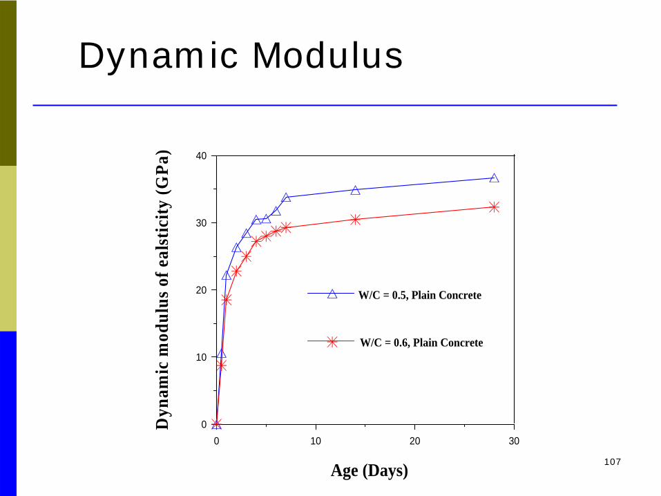
Dynamic Modulus

0 10 20 300

10

20

30

40D

ynam

ic m

odul

us o

f eal

stic

ity (G

Pa)

Age (Days)

W/C = 0.5, Plain Concrete

W/C = 0.6, Plain Concrete

108

0 4 8 12 16 20 24 280

10

20

30

40M

odul

us o

f Ela

stic

ity (M

Pa)

Age (Days)

Static modulus of elasticity

Dynamic modulus of elasticity

Static and dynamic modulus

109

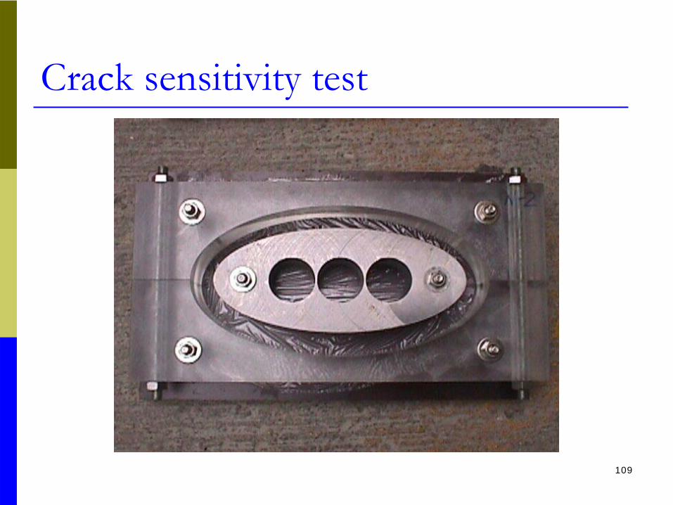
Crack sensitivity test

110

Crack sensitivity test

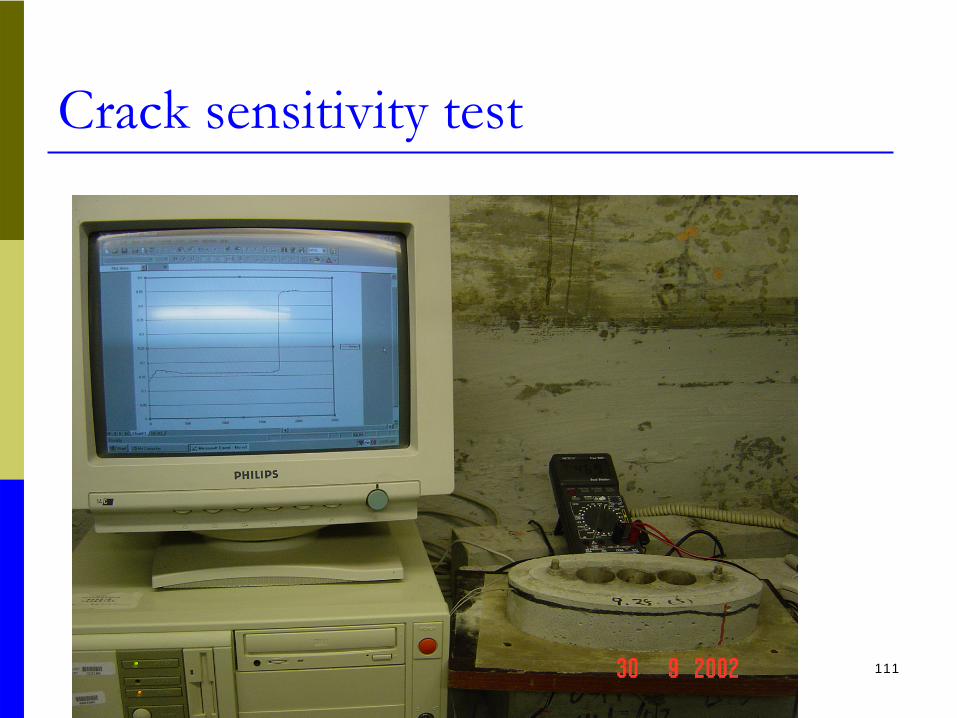
111

Crack sensitivity test

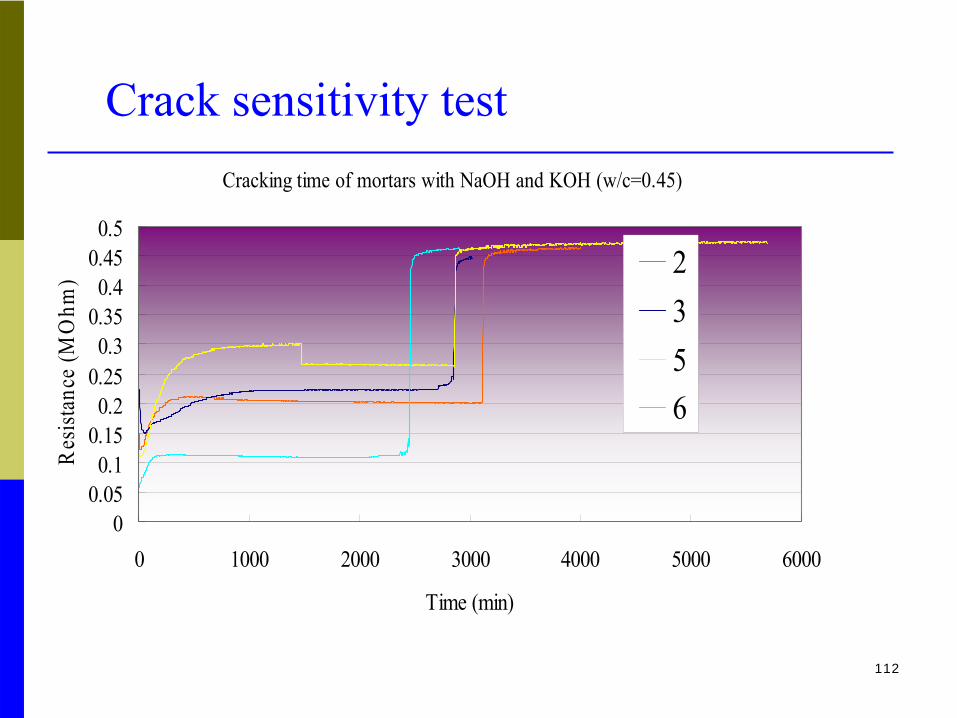
112

Cracking time of mortars with NaOH and KOH (w/c=0.45)

00.050.1

0.150.2

0.250.3

0.350.4

0.450.5

0 1000 2000 3000 4000 5000 6000

Time (min)

Res

istan

ce (M

Ohm

) 2356

Crack sensitivity test

113

THE ENDTHE ENDTHANKS!