Page 1
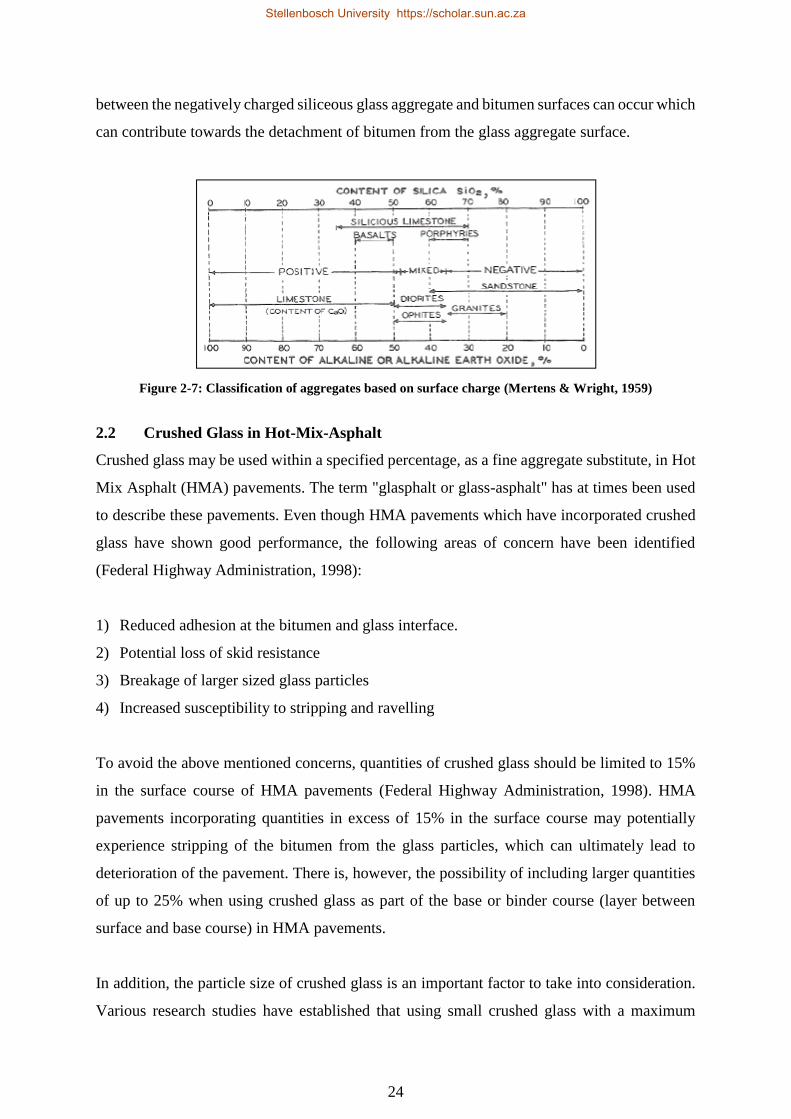
Advanced Characterisation of Hot Mix Asphalt with Recycled Crushed Glass
by
Theresa Bernadette George
Thesis presented in partial fulfillment of the requirement for the degree of Master
of Engineering in Civil Engineering in the Faculty of Engineering at Stellenbosch
University
Department of Civil Engineering
Stellenbosch University
Private Bag
X1 Matieland
7602 South
Africa
Supervisor: Prof. K.J. Jenkins
Co-Supervisors: Dr. J.K. Anochie-Boateng
Assoc. Prof. ir. M.F.C. van de Ven
December 2018
Page 2
i
DECLARATION
By submitting this dissertation, I declare that the entirety of the work contained therein is my
own, original work, that I am the sole author thereof (save to the extent explicitly otherwise
stated), that reproduction and publication thereof by Stellenbosch University will not infringe
any third party rights and that I have not previously in its entirety or in part submitted it for
obtaining any qualification.
Signature:
Date:
Copyright © 2018 Stellenbosch University
All rights reserved
Stellenbosch University https://scholar.sun.ac.za
Page 3
ii
ABSTRACT
Over the last few decades, the use of glass in pavement applications has been implemented by
various countries in the international community. South Africa, however, on average generates
roughly 900 000 tonnes of domestic waste glass each year and has made little use of this readily
available raw material. More recently, with national policies mandating the reuse, recycling
and minimisation of domestic waste, in addition with several economic and environmental
benefits, it is expected that the use of alternative materials, e.g. recycled glass, in road
construction will increase.
Depending on the application, the uses of recycled glass in road construction vary widely. This
study investigates the engineering performance of Hot Mix Asphalt (HMA) incorporating
locally available recycled crushed glass for use in the wearing course of South African
pavements. The study contributes to current research at the Council for Scientific and Industrial
Research (CSIR) which aims to optimise the design, construction and maintenance of roads
through the use of cost-effective and sustainable materials that include waste materials.
A continuously-graded asphalt mix with a glass replacement ratio of 15% and 50/70
penetration grade bitumen was designed for a traffic level of 3 to 30 million E80s. The mix
design was conducted according to the current method for traditional asphalt mixes in South
Africa. The results indicate that the glass-asphalt mix conforms to the South African mix design
criteria.
Furthermore, the moisture susceptibility of the glass-asphalt mix was evaluated with and
without the use of anti-stripping additives. The standard Tensile Strength Ratio parameter
supported with a microscopic imaging technique and an analytical modelling method were
used to evaluate and quantify the resistance of the glass-asphalt mix to moisture damage.
Analysis of the results reveal that an antistripping additive is essential to meet moisture
susceptibility criteria and alleviate stripping for the investigated source and grading of glass
particles, at a glass content of 15%.
The study also assesses and compares the stiffness and permanent deformation properties of
the glass-asphalt mix to a traditional continuously-graded asphalt wearing course mix, typically
used for road construction in South Africa. Selected mathematical models were used to
Stellenbosch University https://scholar.sun.ac.za
Page 4
iii
effectively characterise the deformation and stiffness behaviour of the mixes. The glass-asphalt
mix shows increased stiffness and improved resistance to permanent deformation at elevated
temperatures.
Additionally, a multi-layer linear-elastic analysis is used to assess the influence of temperature
and loading frequency variation on the structural capacity of the glass-asphalt and HMA
surfacing layers. The analysis reveals that the structural capacity of both surfacing layers are
comparable at intermediate temperatures, for both high and low loading frequencies.
The findings of this study reveal that improved performance could potentially be achieved with
the use of recycled crushed glass in continuously-graded asphalt wearing course mixes in South
Africa.
Stellenbosch University https://scholar.sun.ac.za
Page 5
iv
DEDICATION
To my husband for his continuous love and support
Stellenbosch University https://scholar.sun.ac.za
Page 6
v
ACKNOWLEDGEMENTS
I wish to express my gratitude to the following organisations and individuals who assisted and
supported me during this research study:
1. Prof. K.J. Jenkins, Supervisor - Stellenbosch University; for his guidance and support
during the study.
2. Dr. J.K. Anochie-Boateng, Co-supervisor and Project Leader of the CSIR’s project on
glass-asphalt development; for his guidance and support during the study.
3. Assoc. Prof. ir. M.F.C. van de Ven, Co-supervisor - TU Delft; for his guidance and support
during the study.
4. The Council for Scientific and Industrial Research (CSIR) through its R&D office for
funding this research through Parliamentary Grant (PG) Funding - PG project
B1iE201:002.
5. CSIR Pavement Materials and Testing Laboratory staff, in particular Mr. Nnditsheni
Mpofu and Mr. Ngwako Maake, for their assistance during the study.
6. My colleagues in the Pavement Design and Construction research group for valuable
discussions held during the study.
7. Mr. Benoit Verhaeghe, Pavement Design and Construction competency area manager -
CSIR; for his assistance and support during the study.
8. Dr. Martin Mgangira, Pavement Design and Construction research group leader - CSIR;
for his support during the study.
9. Much Asphalt, AfriSam and Consol for providing me with the necessary raw materials
required to conduct the study.
10. My family, most especially my husband and my mom, for helping me with Zion.
11. My husband for his continuous support throughout my Masters study.
12. Above all, my Heavenly Father, for His wisdom, strength and guidance throughout my
Masters study.
Stellenbosch University https://scholar.sun.ac.za
Page 7
vi
LIST OF ABBREVIATIONS
AASHTO - American Association of State Highway and Transportation Officials
AMPT - Asphalt Mixture Performance Tester
ASTM - American Society of Testing Materials
BD - Bulk Density
CSIR - Council for Scientific and Industrial research
FAA - Fine Aggregate Angularity
GHG - Greenhouse Gas Emissions
HMA - Hot Mix Asphalt
HWTT - Hamburg Wheel Tracking Test
ITS - Indirect Tensile Strength
LVE - Linear-Viscoelastic
MPS - Maximum Particle Size
MVD - Maximum Voidless Density
NEM: WA - National Environmental Management: Waste Act
NEMA - National Environmental Management Act
NMPS - Nominal Maximum Particle Size
NWMS - National Waste Management Strategy
PRO - Producer Responsibility Organisation
R&D - Research and Development
RTFOT - Rolling Thin Film Oven Test
SANRAL - South African National Roads Agency Limited
SANS - South African National Standards
SAPDM - South African Pavement Design Method
SEM - Scanning Electron Microscopy
SHRP - Strategic Highway Research Program
TGRC - The Glass Recycling Company
TSR - Tensile Strength Ratio
VFB - Voids Filled with Binder
VIM - Voids in Mix
VMA - Voids in Mineral Aggregate
XRD - X-Ray Diffraction
XRF - X-Ray Fluorescence
Stellenbosch University https://scholar.sun.ac.za
Page 8
vii
TABLE OF CONTENTS
1. INTRODUCTION .............................................................................................................. 1
1.1 Background ................................................................................................................. 1
1.2 Problem Statement ...................................................................................................... 3
1.3 Research Goal and Objectives..................................................................................... 3
1.3.1. Research Goal ...................................................................................................... 3
1.3.2. Research Objectives ............................................................................................. 3
1.4 Research Scope ........................................................................................................... 4
1.5 Outline of Dissertation ................................................................................................ 4
2. LITERATURE STUDY ..................................................................................................... 6
2.1 Introduction ................................................................................................................. 6
2.1.1 Domestic Waste Glass ......................................................................................... 6
2.1.2 Domestic Waste Glass Management in South Africa .......................................... 7
2.1.3 Sources of Recycled Crushed Glass in South Africa ........................................... 8
2.1.4 Global Utilisation of Crushed Glass in Pavement Applications ........................ 13
2.1.5 Material Properties of Recycled Crushed Glass ................................................ 17
2.2 Crushed Glass in Hot-Mix-Asphalt ........................................................................... 24
2.3 Summary ................................................................................................................... 46
3. GLASS-ASPHALT MIX DESIGN .................................................................................. 48
3.1. Introduction ............................................................................................................... 48
3.2. Raw Materials ........................................................................................................... 49
3.2.1. Aggregate ........................................................................................................... 49
3.2.2. Filler ................................................................................................................... 51
3.2.3. Bituminous Binder ............................................................................................. 51
3.2.4. Antistripping Additives ...................................................................................... 52
3.3. Aggregate Design ...................................................................................................... 52
3.4. Minimum Binder Content ......................................................................................... 55
Stellenbosch University https://scholar.sun.ac.za
Page 9
viii
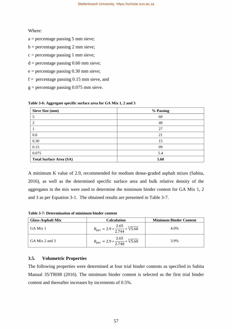
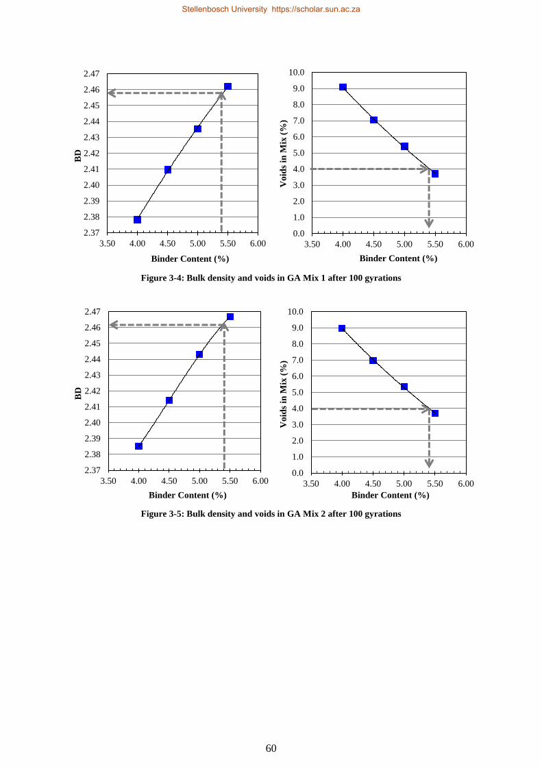
3.5. Volumetric Properties ............................................................................................... 57
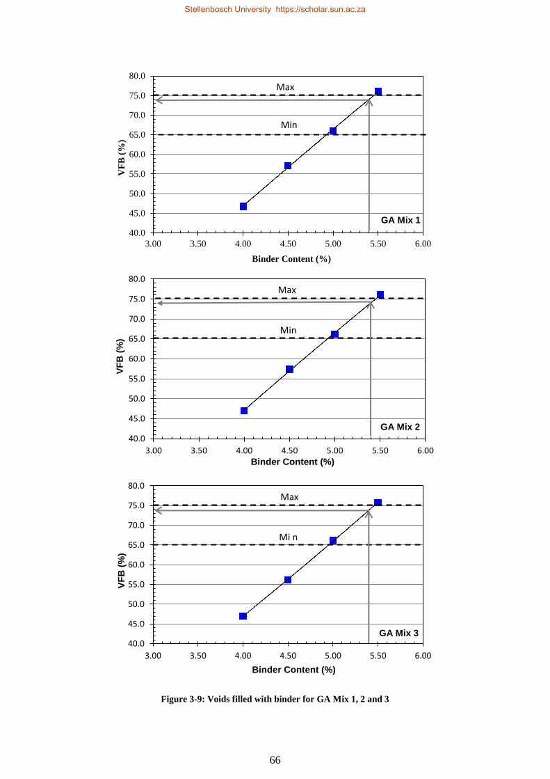
3.5.1. Maximum Voidless Density (MVD) ................................................................. 58
3.5.2. Bulk Density (BD), Voids in Mix (VIM) and Optimum Binder Content .......... 58
3.5.3. Voids in Mineral Aggregate (VMA).................................................................. 62
3.5.4. Voids Filled with Binder (VFB) ........................................................................ 65
3.6. Mixing, Ageing, Compaction and Specimen Preparation ......................................... 67
3.6.1. Mechanical Mixing ............................................................................................ 67
3.6.2. Short-term Oven Ageing .................................................................................... 67
3.6.3. Gyratory Compaction......................................................................................... 67
3.6.4. Specimen Preparation ........................................................................................ 67
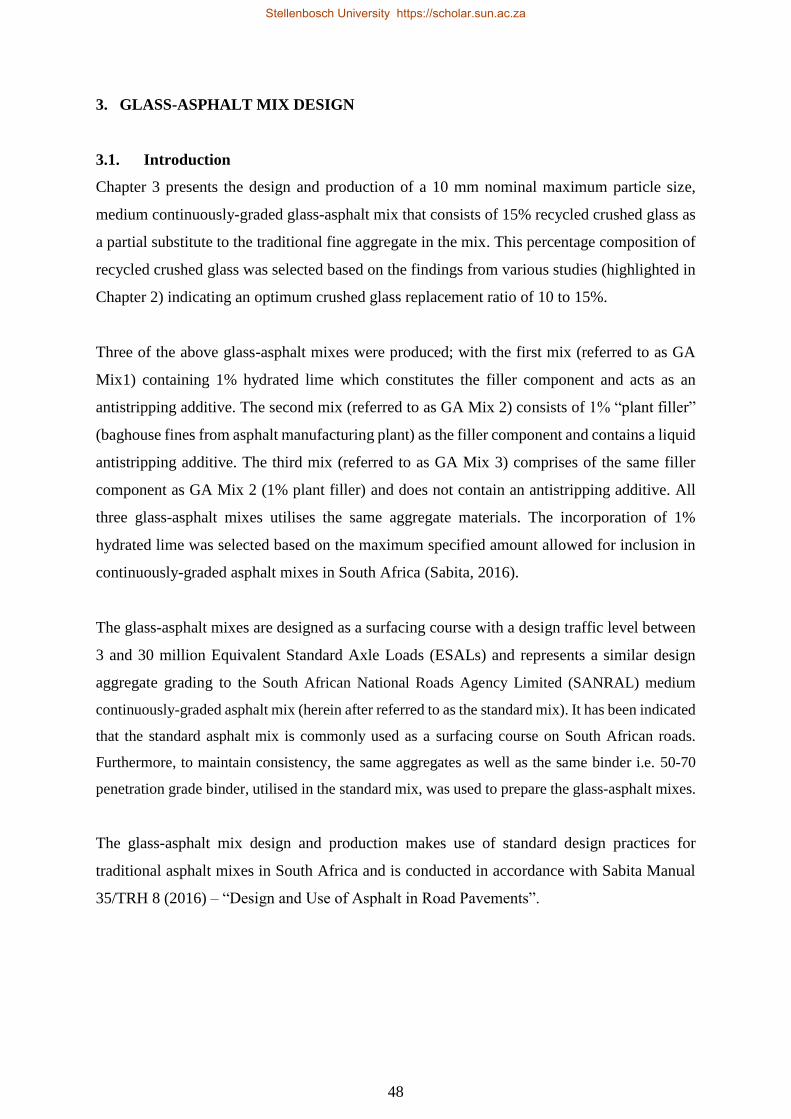
3.7. Physical Characterisation of Aggregate and Recycled Crushed Glass ..................... 68
3.7.1. Bulk Density (BD) ............................................................................................. 68
3.7.2. Water Absorption ............................................................................................... 68
3.7.3. Fine Aggregate Angularity (FAA) ..................................................................... 69
3.7.4. Sand Equivalency............................................................................................... 70
3.7.5. X-Ray Diffraction (XRD) Analysis of Waste Glass Material ........................... 72
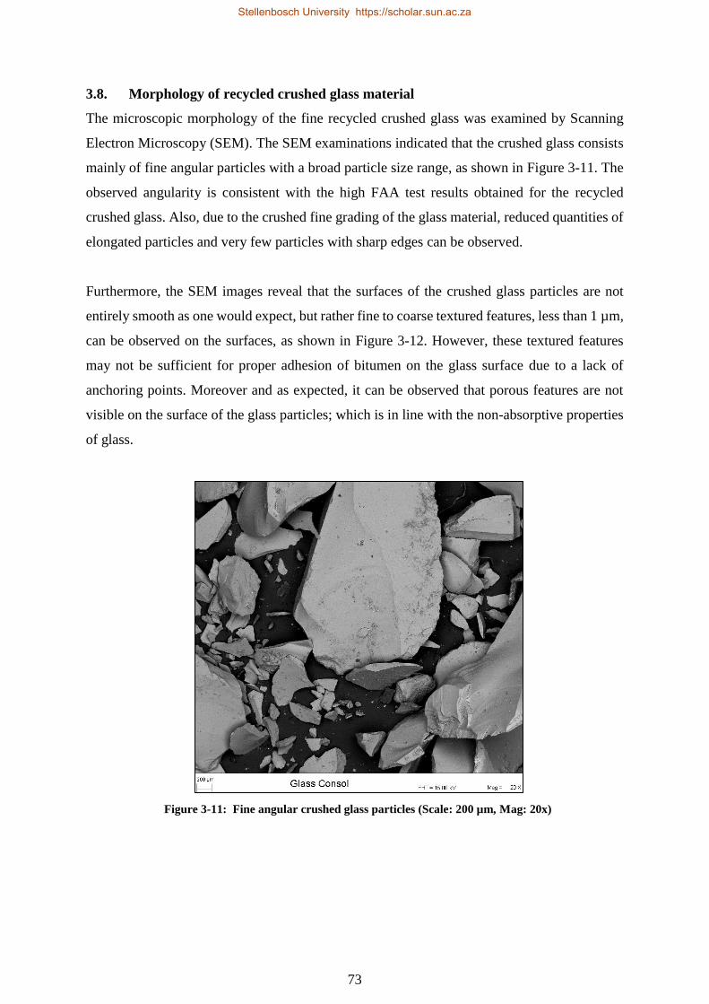
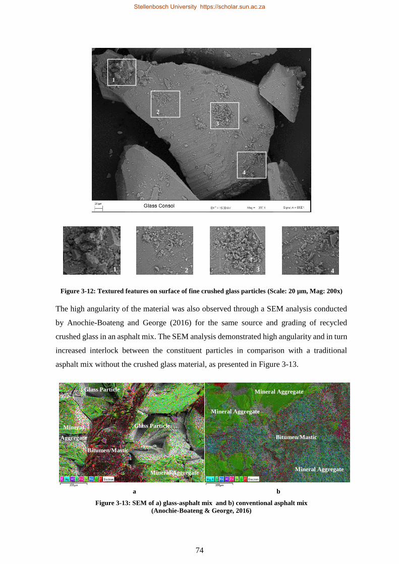
3.8. Morphology of recycled crushed glass material ....................................................... 73
3.9. Summary ................................................................................................................... 75
4. SELECTION OF OPTIMUM GLASS-ASPHALT MIX ................................................. 76
4.1. Introduction ............................................................................................................... 76
4.2. Moisture Susceptibility Evaluation of Glass-Asphalt Mixes Using Modified Lottman
Test ............................................................................................................................ 76
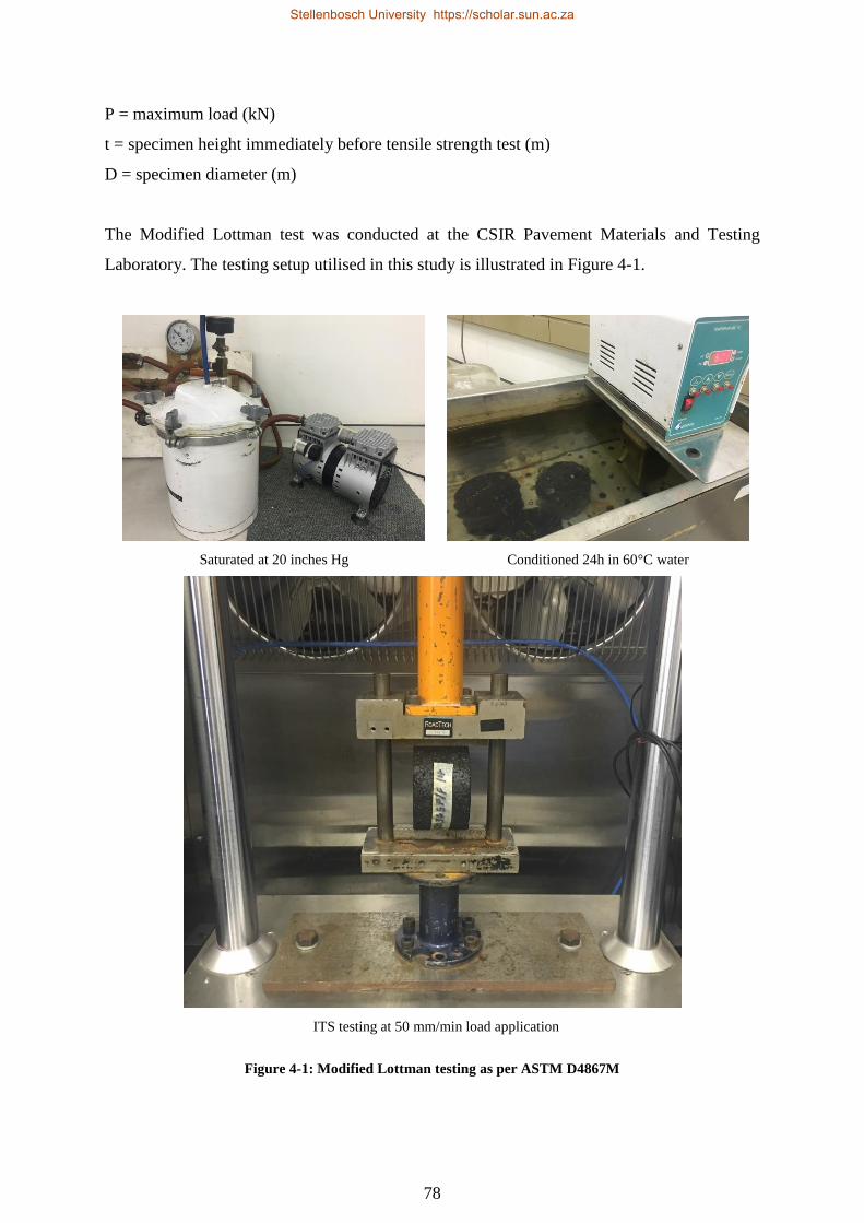
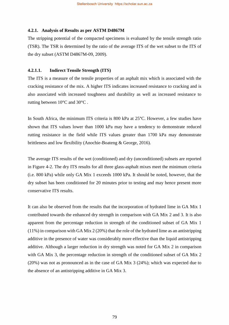
4.2.1. Analysis of Results as per ASTM D4867M ...................................................... 79
4.2.1.1. Indirect Tensile Strength (ITS) .......................................................................... 79
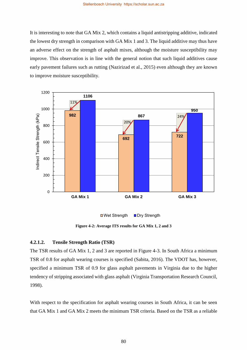
4.2.1.2. Tensile Strength Ratio (TSR)............................................................................. 80
4.2.1.3. Visual Estimation of Moisture Damage ............................................................. 83
4.2.2. Moisture Damage Evaluation Using Image Analysis Techniques .................... 83
Stellenbosch University https://scholar.sun.ac.za
Page 10
ix
4.3. Moisture Susceptibility Evaluation of Glass-Asphalt Mixes Using Hamburg Wheel
Tracking Test............................................................................................................. 91
4.3.1. Current HWTT Analysis Methodology as per AASHTO T 324 ....................... 92
4.3.2. Proposed New HWTT Analysis Methodology .................................................. 95
4.4. Summary ................................................................................................................. 105
5. PERFORMANCE EVALUATION OF OPTIMUM GLASS-ASPHALT MIX ............ 107
5.1. Introduction ............................................................................................................. 107
5.2. Reference Mix ......................................................................................................... 107
5.2.1. Design Aggregate Grading .............................................................................. 107
5.2.2. Minimum Binder Content ................................................................................ 108
5.2.3. Voids in Mix (VIM) and Optimum Binder Content ........................................ 108
5.3. Permanent Deformation Evaluation ........................................................................ 111
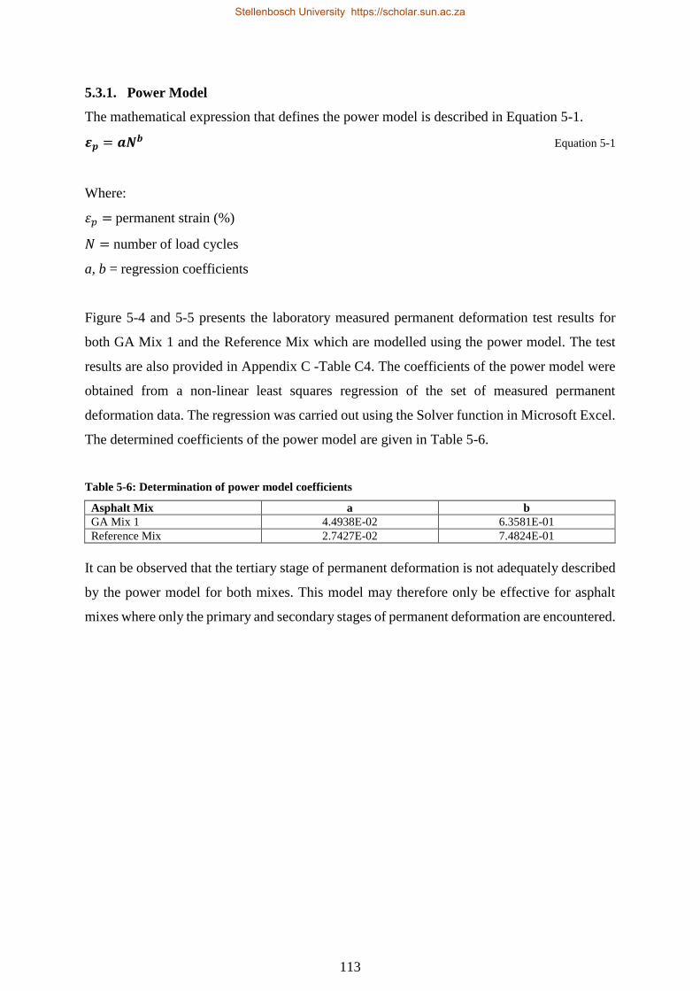
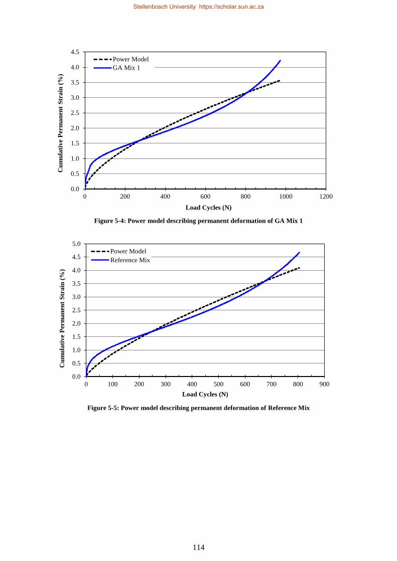
5.3.1. Power Model .................................................................................................... 113
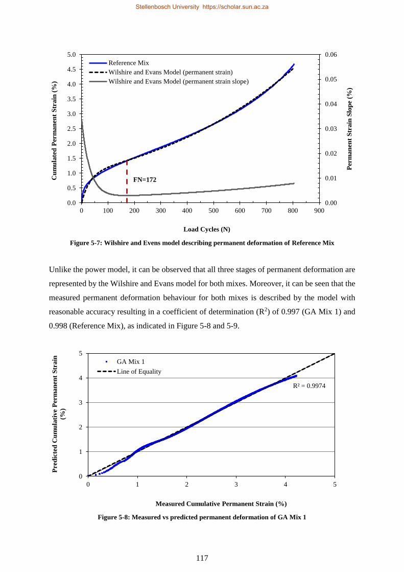
5.3.2. Wilshire and Evans Model ............................................................................... 115
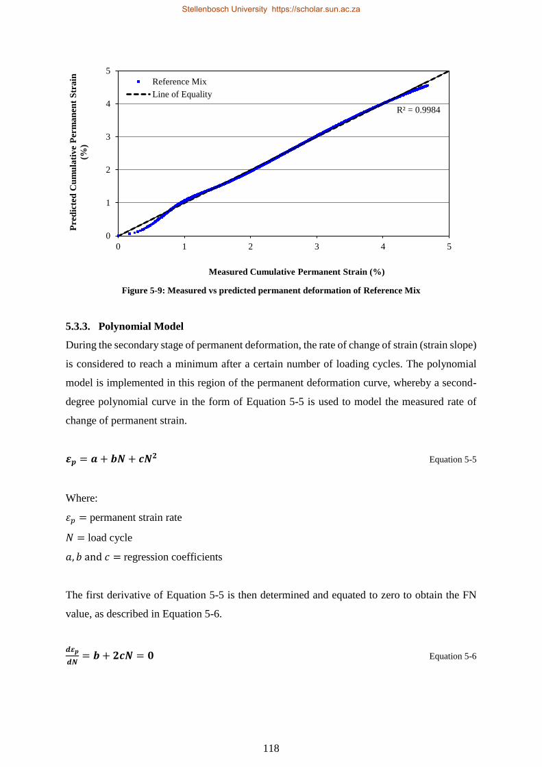
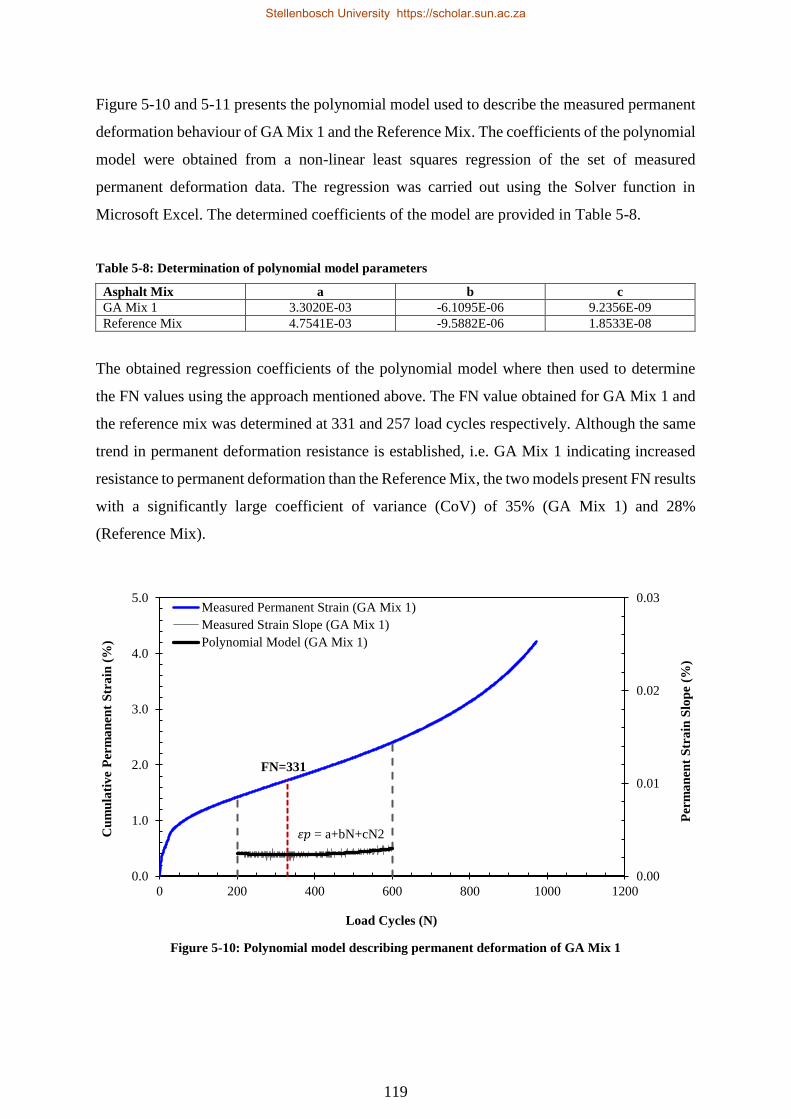
5.3.3. Polynomial Model ............................................................................................ 118
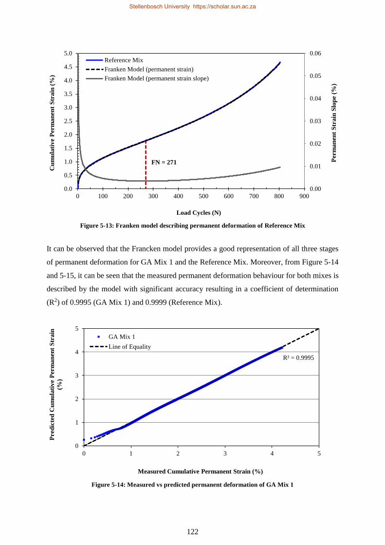
5.3.4. Francken Model ............................................................................................... 120
5.4. Stiffness Evaluation................................................................................................. 124
5.4.1. Dynamic Modulus Test Results and Analysis ................................................. 124
5.5. Modelling the Linear-Viscoelastic (LVE) Behaviour of Glass-Asphalt ................. 131
5.5.1. Constitutive Models ......................................................................................... 134
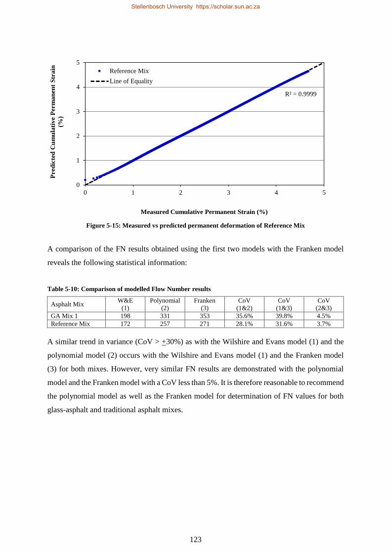
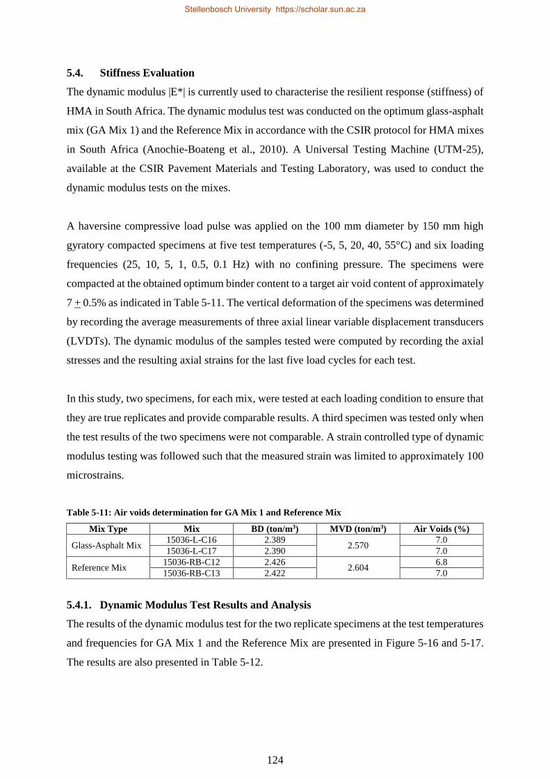
5.5.2. Analysis of Results .......................................................................................... 140
5.6. Summary ................................................................................................................. 147
6. STRUCTURAL PERFORMANCE EVALUATION OF GLASS-ASPHALT
SURFACING PAVEMENTS......................................................................................... 148
6.1. Introduction ............................................................................................................. 148
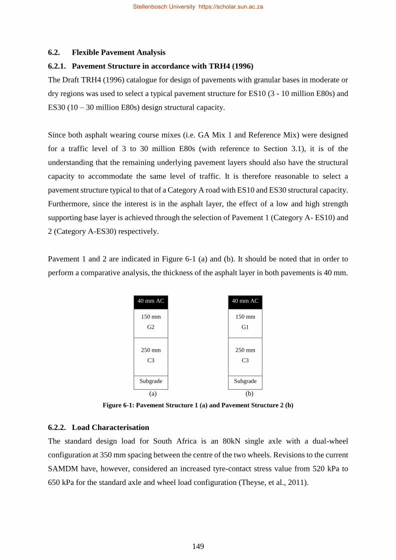
6.2. Flexible Pavement Analysis .................................................................................... 149
6.2.1. Pavement Structure in accordance with TRH4 (1996) .................................... 149
6.2.2. Load Characterisation ...................................................................................... 149
Stellenbosch University https://scholar.sun.ac.za
Page 11
x
6.2.3. Material Characterisation ................................................................................. 150
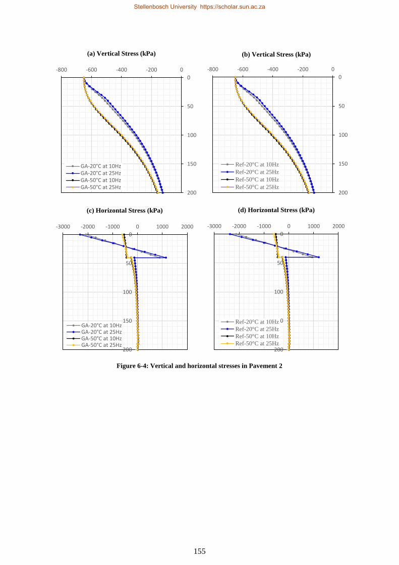
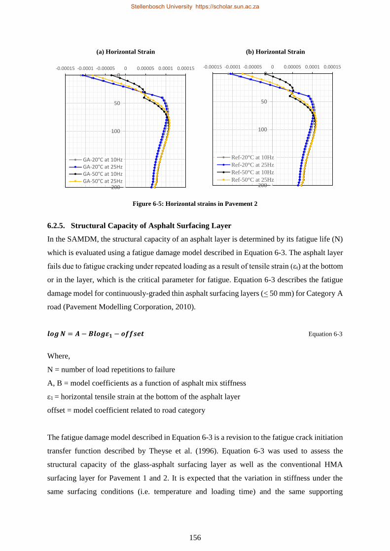
6.2.4. Stress-Strain Behaviour ................................................................................... 151
6.2.5. Structural Capacity of Asphalt Surfacing Layer .............................................. 156
6.2.6. Structural Capacity of Subgrade Layer ............................................................ 159
6.3. Summary ................................................................................................................. 162
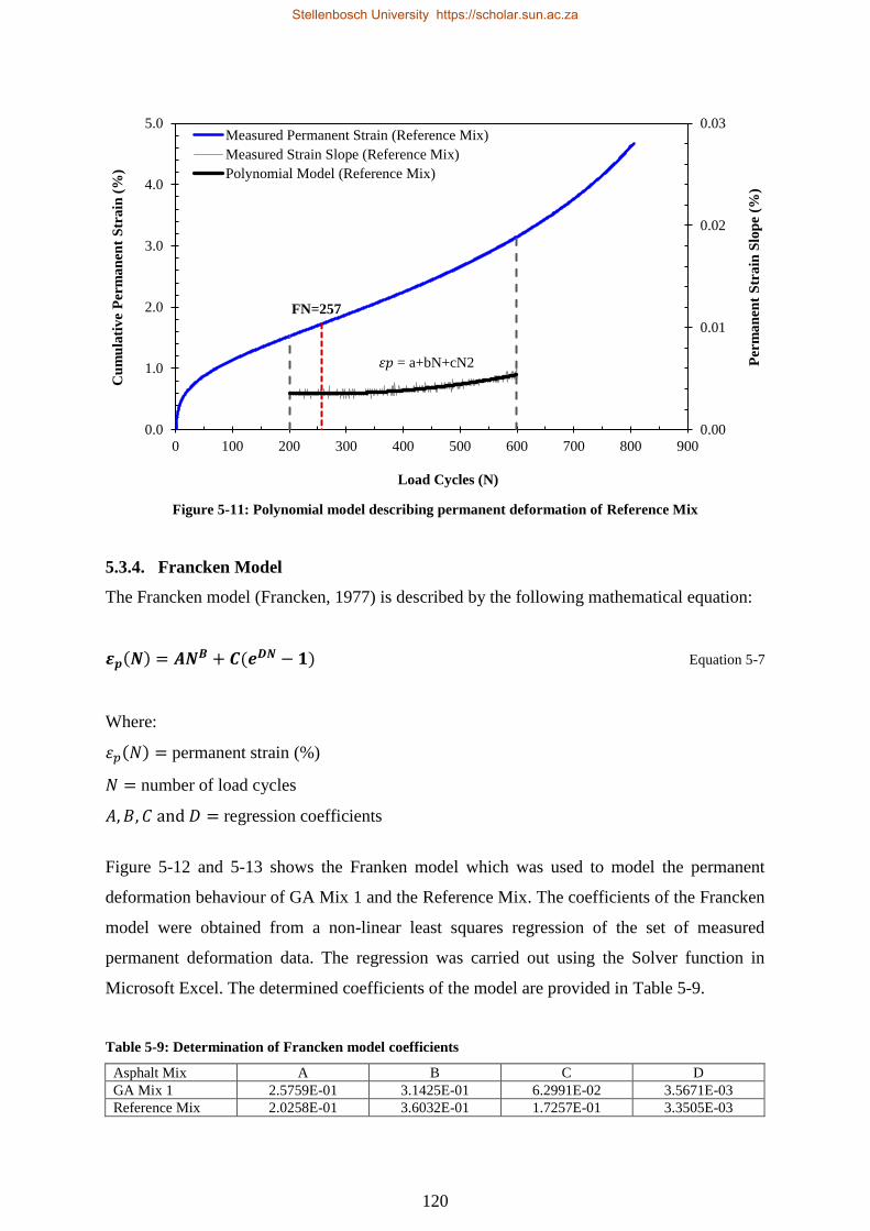
7. CONCLUSIONS AND RECOMMENDATIONS ......................................................... 164
7.1. Conclusions ............................................................................................................. 164
7.2. Recommendations ................................................................................................... 166
8. REFERENCES ............................................................................................................... 168
APPENDIX A: VOLUMETRIC TEST DATA ..................................................................... 176
APPENDIX B: MODIFIED LOTTMAN AND HWTT TEST DATA ................................. 181
APPENDIX C: FLOW NUMBER TEST DATA .................................................................. 188
Stellenbosch University https://scholar.sun.ac.za
Page 12
xi
LIST OF TABLES
Table 2-1: Thermal Conductivity Test Results ........................................................................ 20
Table 2-2: Typical chemical composition of soda-lime glass ................................................. 21
Table 2-3: Adhesive bond energy per unit area of sample (ergs/cm2) (Cheng et al., 2002) .... 23
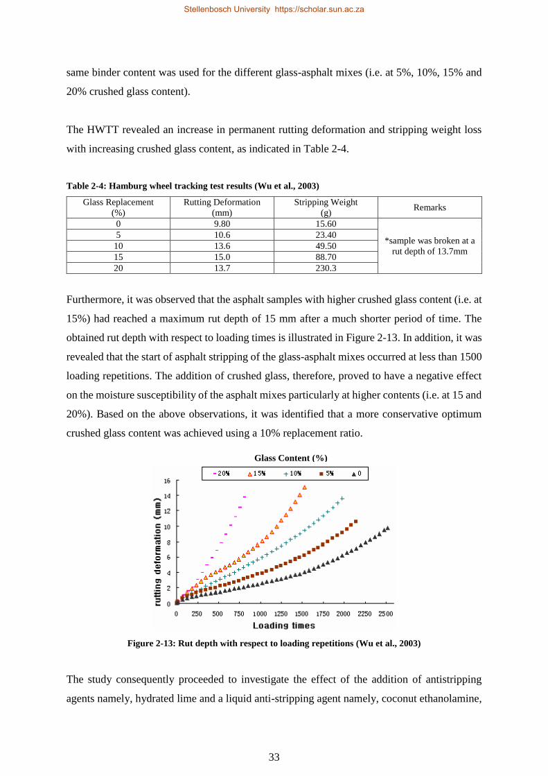
Table 2-4: Hamburg wheel tracking test results (Wu et al., 2003) .......................................... 33
Table 2-5: Design grading of glass-asphalt mix (Arabani, 2010) ............................................ 39
Table 3-1: Aggregate Material and Sources ............................................................................ 49
Table 3-2: Properties of the 50-70 Penetration Grade Binder ................................................. 52
Table 3-3: Aggregate design for GA Mix 1, 2 and 3 ............................................................... 54
Table 3-4: Bulk density of aggregate in GA Mix 1 ................................................................. 56
Table 3-5: Bulk density of aggregate in GA Mix 2 & 3 .......................................................... 56
Table 3-6: Aggregate specific surface area for GA Mix 1, 2 and 3 ......................................... 57
Table 3-7: Determination of minimum binder content ............................................................ 57
Table 3-8: MVD results at each trial binder content for GA Mix 1, 2 and 3 ........................... 58
Table 3-9: Bulk density and voids in GA Mix 1, 2 and 3 after 100 gyrations ......................... 61
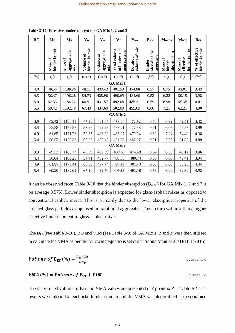
Table 3-10: Effective binder content for GA Mix 1, 2 and 3 .................................................. 63
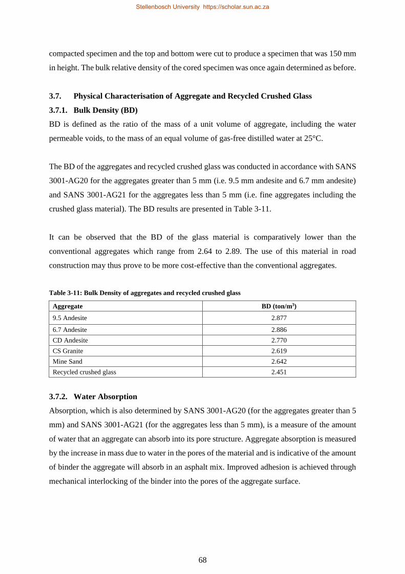
Table 3-11: Bulk Density of aggregates and recycled crushed glass ....................................... 68
Table 3-12: Aggregate and recycled crushed glass absorption ................................................ 69
Table 3-13: Angularity of fine aggregates and recycled crushed glass ................................... 70
Table 3-14: Sand equivalent values for fine aggregate and recycled crushed glass ................ 71
Table 3-15: XRD test results .................................................................................................... 72
Table 3-16: Design and Production of Glass-Asphalt Mixes .................................................. 75
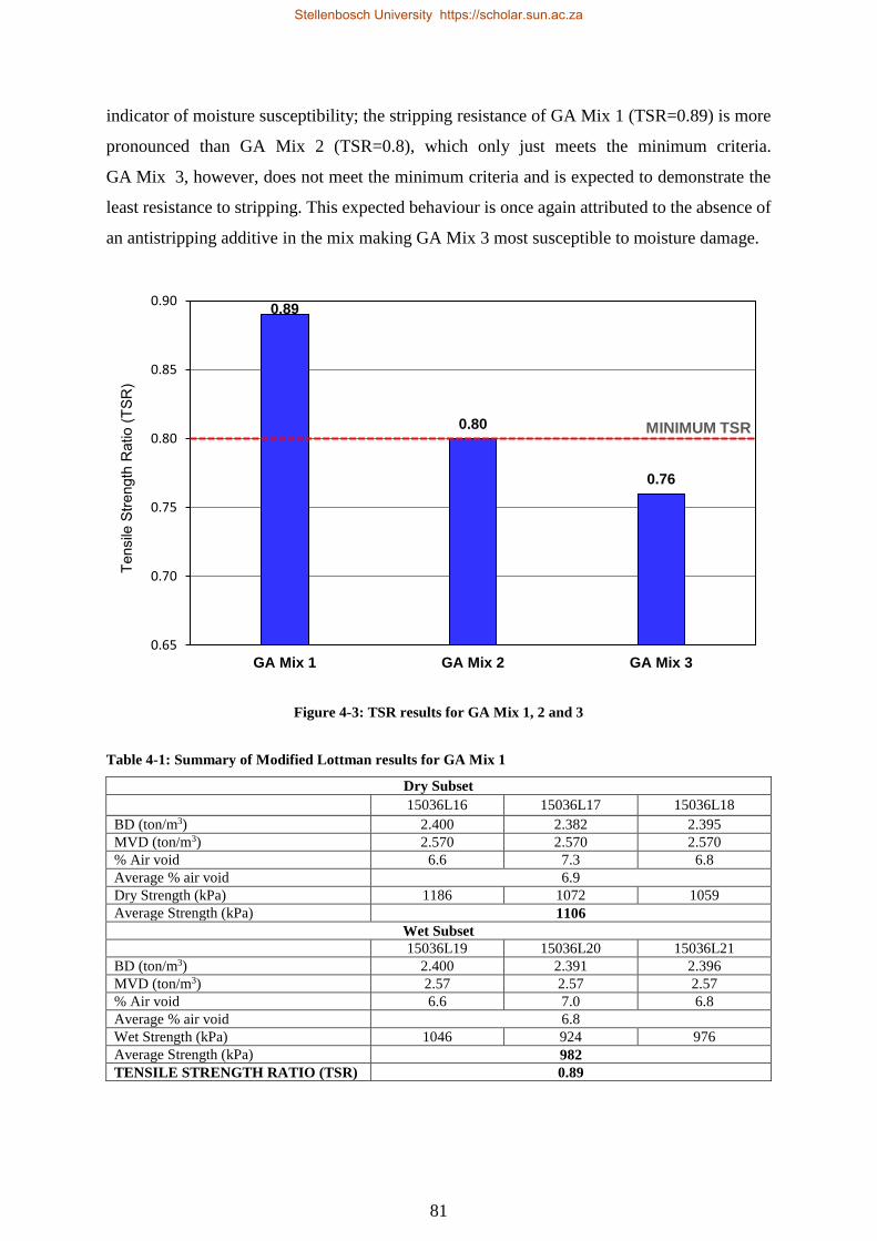
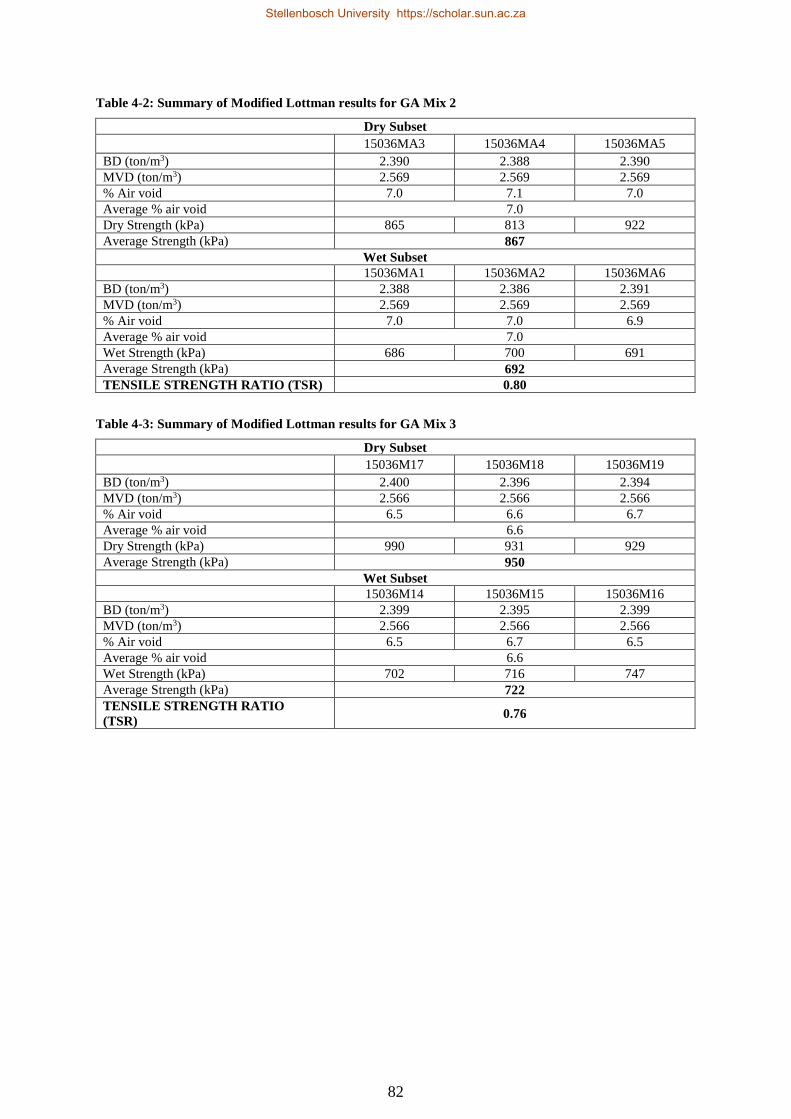
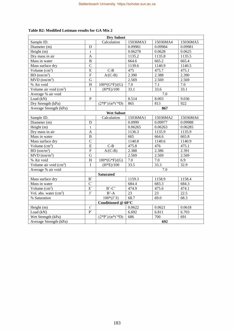
Table 4-1: Summary of Modified Lottman results for GA Mix 1 ........................................... 81
Table 4-2: Summary of Modified Lottman results for GA Mix 2 ........................................... 82
Table 4-3: Summary of Modified Lottman results for GA Mix 3 ........................................... 82
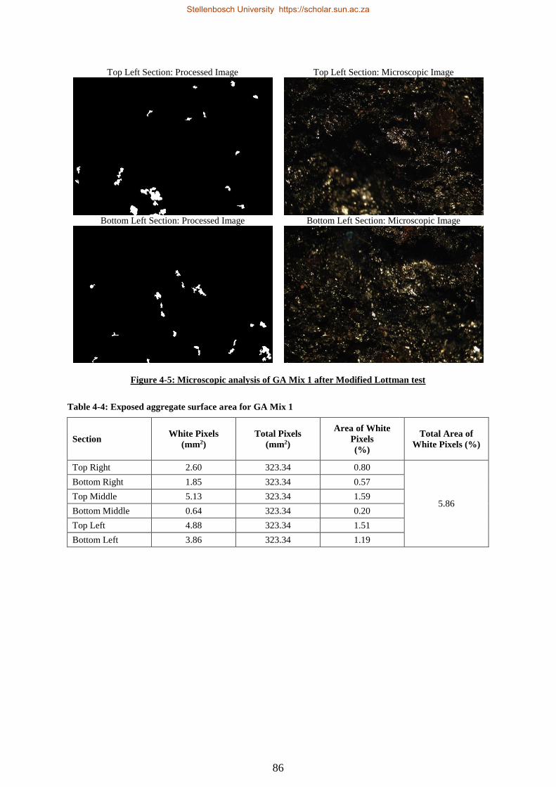
Table 4-4: Exposed aggregate surface area for GA Mix 1 ...................................................... 86
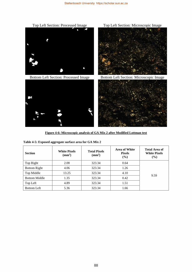
Table 4-5: Exposed aggregate surface area for GA Mix 2 ...................................................... 88
Table 4-6: Exposed aggregate surface area for GA Mix 3 ...................................................... 90
Table 4-7: Determination of air void content for GA Mix 1, 2 and 3 ...................................... 92
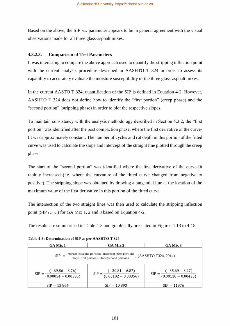
Table 4-8: Determination of SIP as per AASHTO T 324 ...................................................... 101
Table 4-9: Moisture susceptibility ranking for GA Mix 1, 2 and 3 ....................................... 105
Table 5-1: Minimum binder content for Reference Mix ....................................................... 108
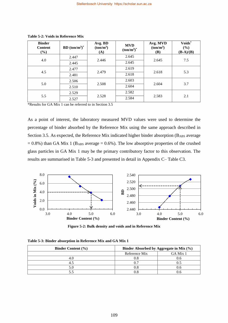
Table 5-2: Voids in Reference Mix ....................................................................................... 109
Stellenbosch University https://scholar.sun.ac.za
Page 13
xii
Table 5-3: Binder absorption in Reference Mix and GA Mix 1 ............................................ 109
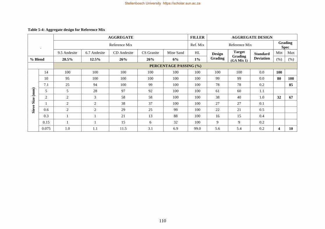
Table 5-4: Aggregate design for Reference Mix ................................................................... 110
Table 5-5: Air voids determination for GA Mix 1 and Reference Mix ................................. 112
Table 5-6: Determination of power model coefficients ......................................................... 113
Table 5-7: Determination of Wilshire and Evans model parameters ..................................... 115
Table 5-8: Determination of polynomial model parameters .................................................. 119
Table 5-9: Determination of Francken model coefficients .................................................... 120
Table 5-10: Comparison of modelled Flow Number results ................................................. 123
Table 5-11: Air voids determination for GA Mix 1 and Reference Mix ............................... 124
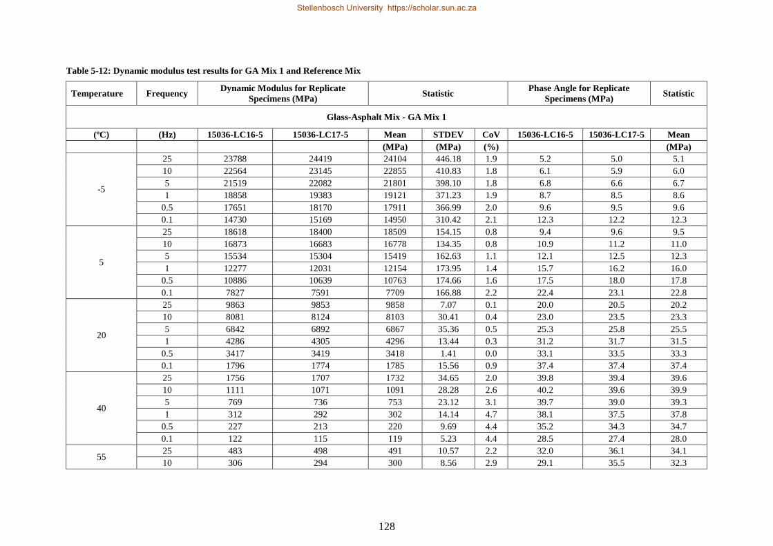
Table 5-12: Dynamic modulus test results for GA Mix 1 and Reference Mix ...................... 128
Table 5-13: Summary of viscosity-temperature regression results ....................................... 137
Table 5-14: Determination of sigmoidal model parameters .................................................. 141
Table 5-15: Determination of Burger’s model parameters .................................................... 141
Table 5-16: Determination of Huet-Sayegh model parameters ............................................. 144
Table 6-1: Huet-Sayegh model parameters for GA Mix 1 and Reference Mix ..................... 150
Table 6-2: Dynamic moduli for GA Mix 1 and Reference Mix ............................................ 150
Table 6-3: Material properties for base and subbase layers of Pavement 1 and Pavement 2 151
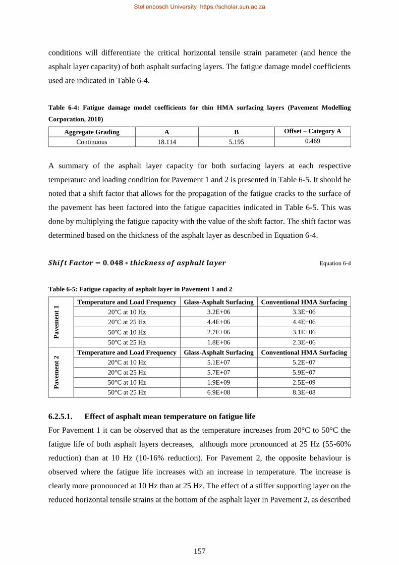
Table 6-4: Fatigue damage model coefficients for thin HMA surfacing layers ................... 157
Table 6-5: Fatigue capacity of asphalt layer in Pavement 1 and 2 ........................................ 157
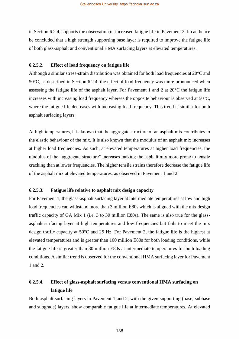
Table 6-6: Vertical compressive strain at top of asphalt layer ............................................... 159
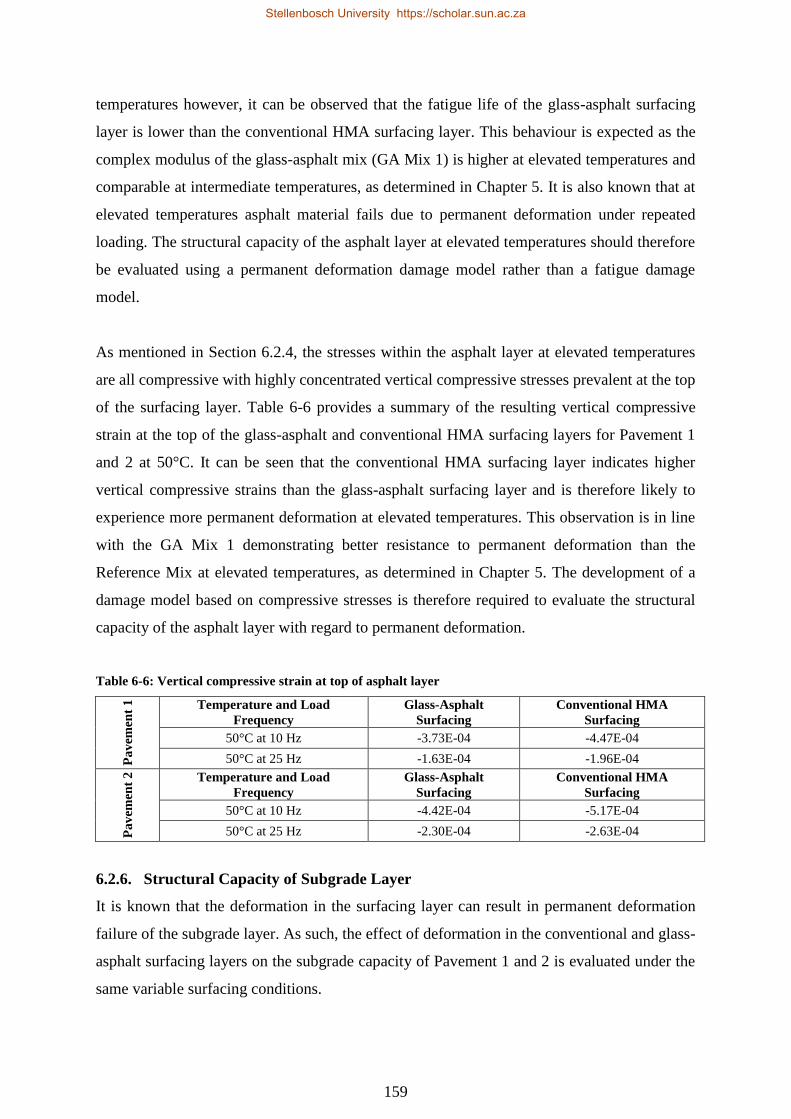
Table 6-7: Subgrade layer capacity in Pavement 1 and 2 ...................................................... 160
Table 6-8: Variable asphalt surfacing parameters ................................................................. 162
Stellenbosch University https://scholar.sun.ac.za
Page 14
xiii
LIST OF FIGURES
Figure 2-1: General waste composition, 2011 (percentage by mass) ........................................ 6
Figure 2-2: Waste glass recycling operations at Consol .......................................................... 12
Figure 2-3: Countries using waste glass in pavement applications ......................................... 13
Figure 2-4: Schematic representation of the bitumen-aggregate-water phase system ............. 18
Figure 2-5: Particle size distribution of recycled crushed glass from Consol ......................... 19
Figure 2-6: Acid-base composition of typical aggregates ....................................................... 22
Figure 2-7: Classification of aggregates based on surface charge ........................................... 24
Figure 2-8: Schematic representation of typical amine groups ............................................... 26
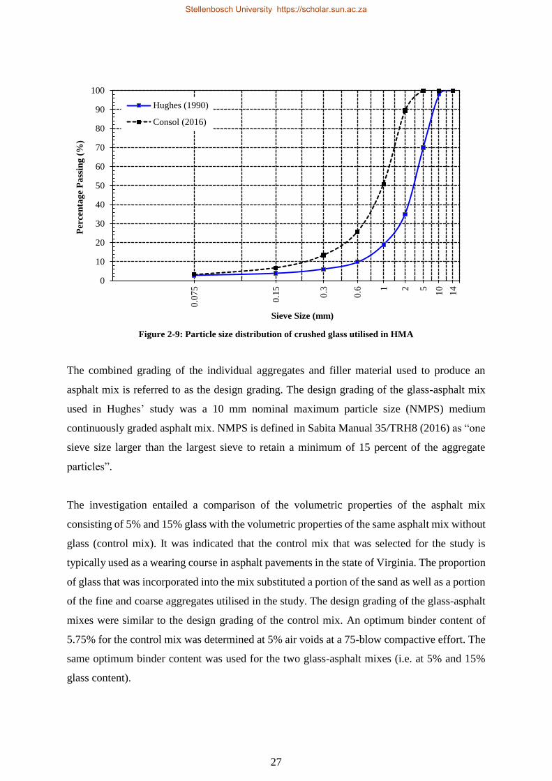
Figure 2-9: Particle size distribution of crushed glass utilised in HMA .................................. 27
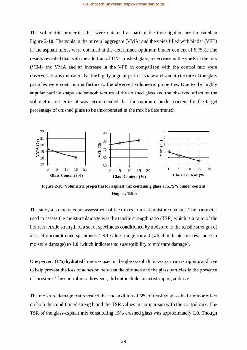
Figure 2-10: Volumetric properties for glass-asphalt mix ....................................................... 28
Figure 2-11: 10 mm (left) and 5 mm (right) maximum glass particle size in asphalt mix ...... 31
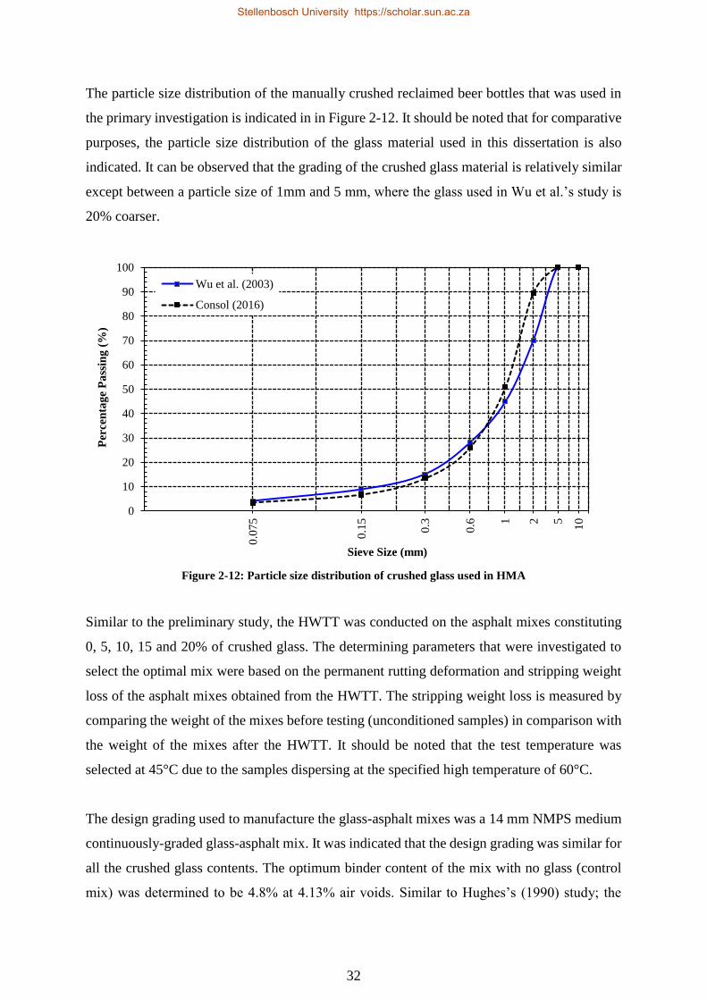
Figure 2-12: Particle size distribution of crushed glass used in HMA .................................... 32
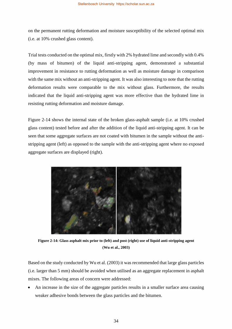
Figure 2-13: Rut depth with respect to loading repetitions (Wu et al., 2003) ......................... 33
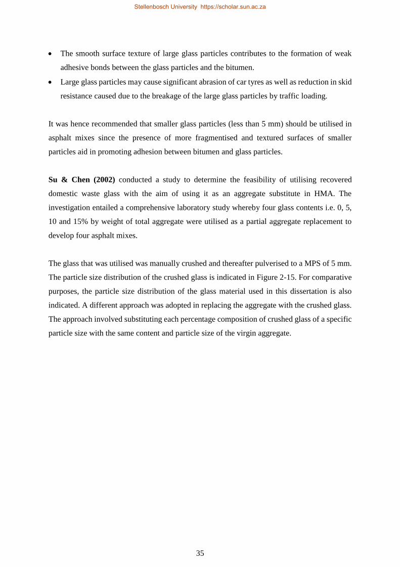
Figure 2-14: Glass asphalt mix prior to (left) and post (right) use of anti-stripping agent ...... 34
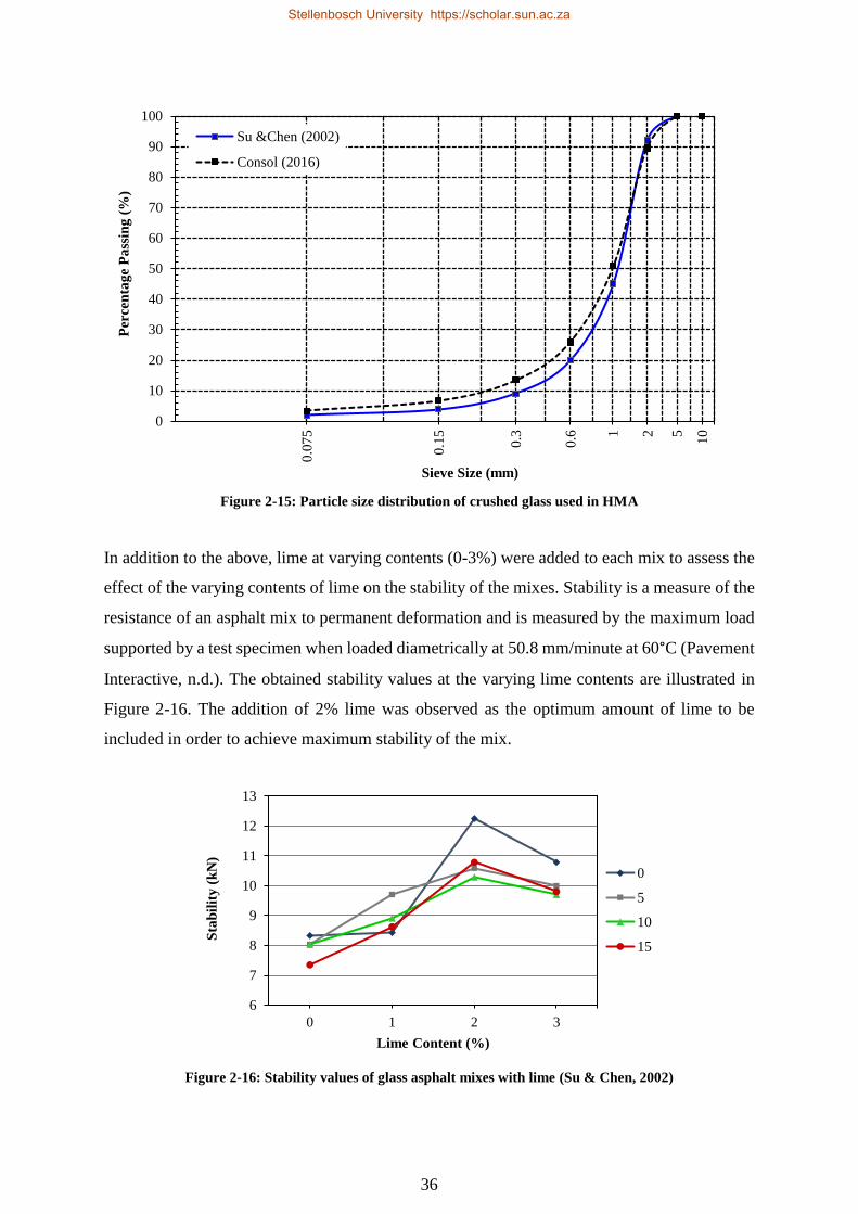
Figure 2-15: Particle size distribution of crushed glass used in HMA .................................... 36
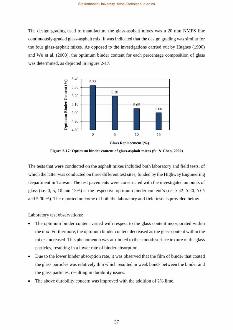
Figure 2-16: Stability values of glass asphalt mixes with lime (Su & Chen, 2002) ................ 36
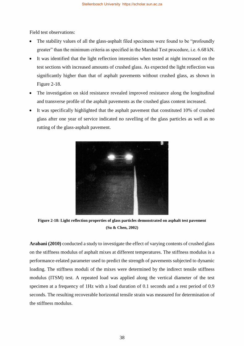
Figure 2-17: Optimum binder content of glass-asphalt mixes (Su & Chen, 2002) ................. 37
Figure 2-18: Light reflection properties of glass particles ....................................................... 38
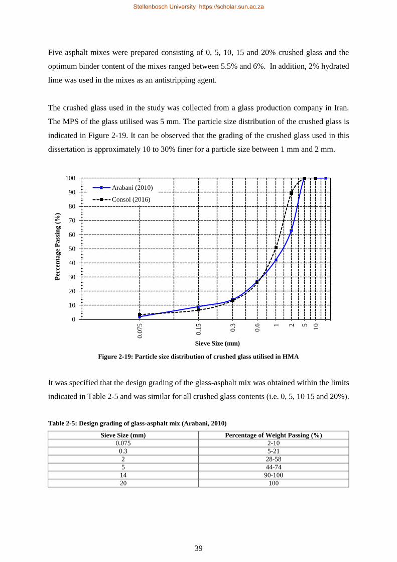
Figure 2-19: Particle size distribution of crushed glass utilised in HMA ................................ 39
Figure 2-20: Variations of stiffness modulus with temperature .............................................. 41
Figure 2-21: Different sizes of crushed glass used (Lachance-Tremblay et al., 2014) ........... 42
Figure 3-1: Photographs of recycled crushed glass particles retained on standard sieve size . 50
Figure 3-2: Particle size distribution of individual aggregate fractions ................................... 51
Figure 3-3: Design grading of 10 mm NMPS GA Mix 1, 2 & 3 ............................................. 55
Figure 3-4: Bulk density and voids in GA Mix 1 after 100 gyrations ..................................... 60
Figure 3-5: Bulk density and voids in GA Mix 2 after 100 gyrations ..................................... 60
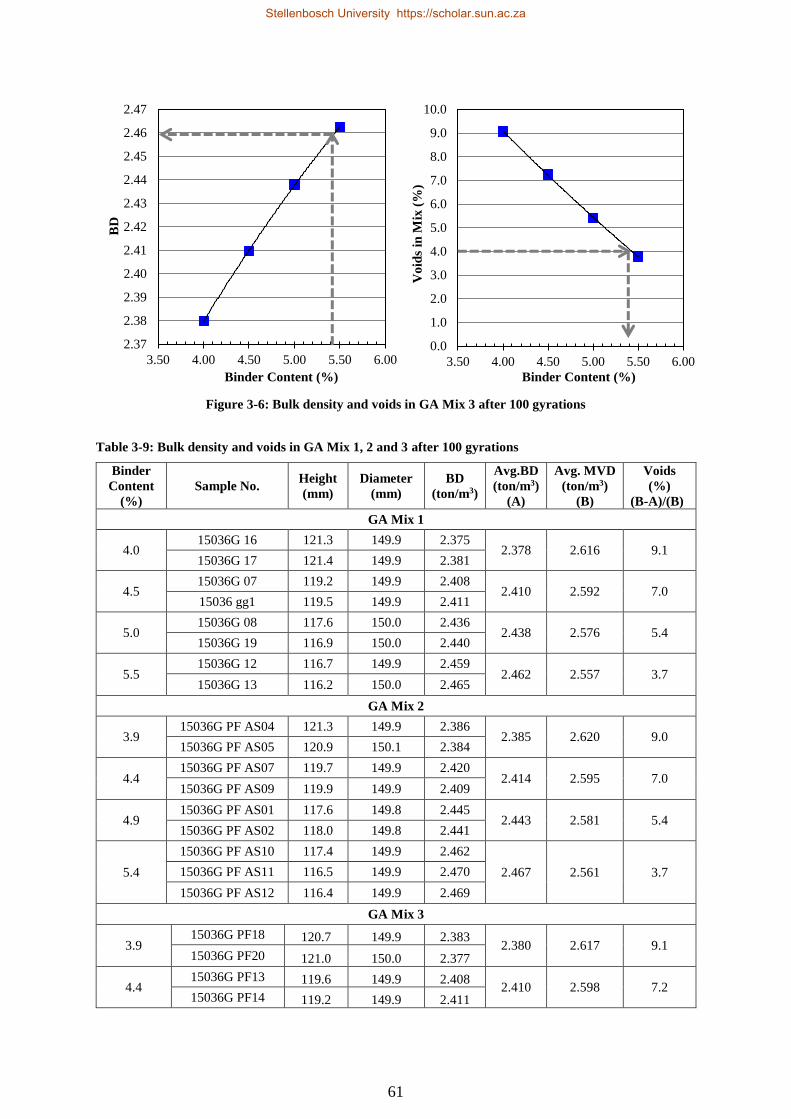
Figure 3-6: Bulk density and voids in GA Mix 3 after 100 gyrations ..................................... 61
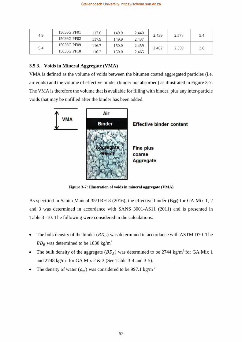
Figure 3-7: Illustration of voids in mineral aggregate (VMA) ................................................ 62
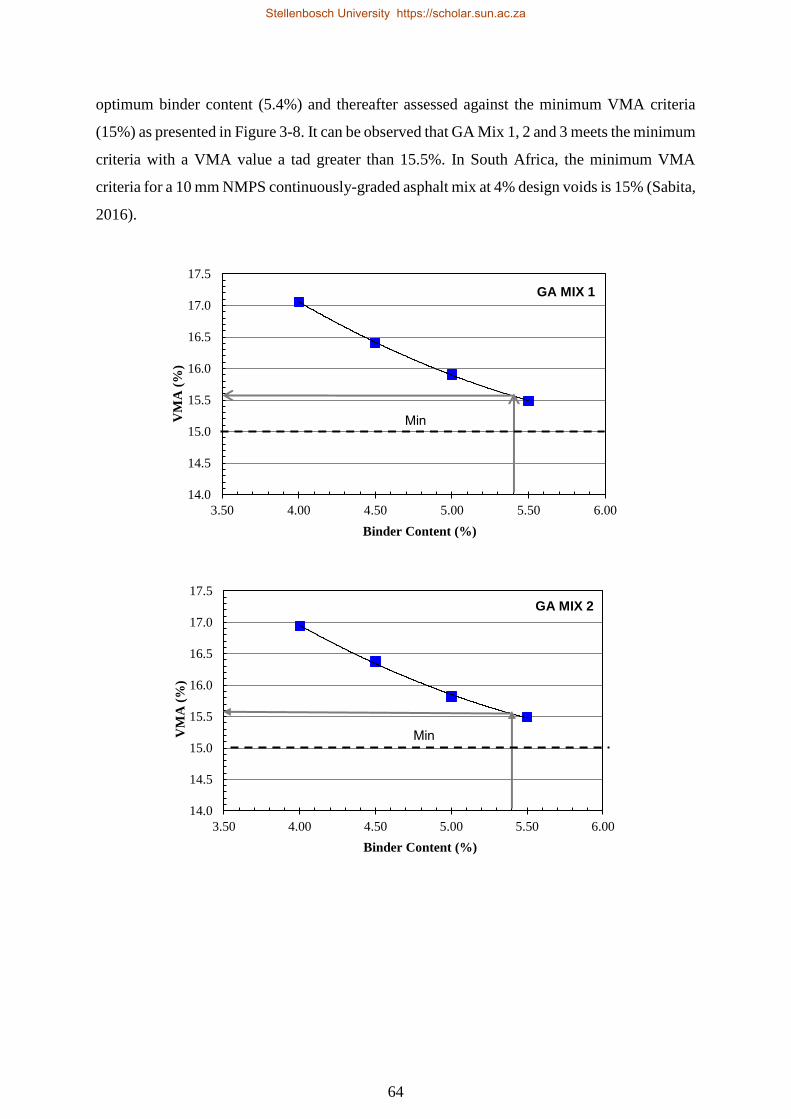
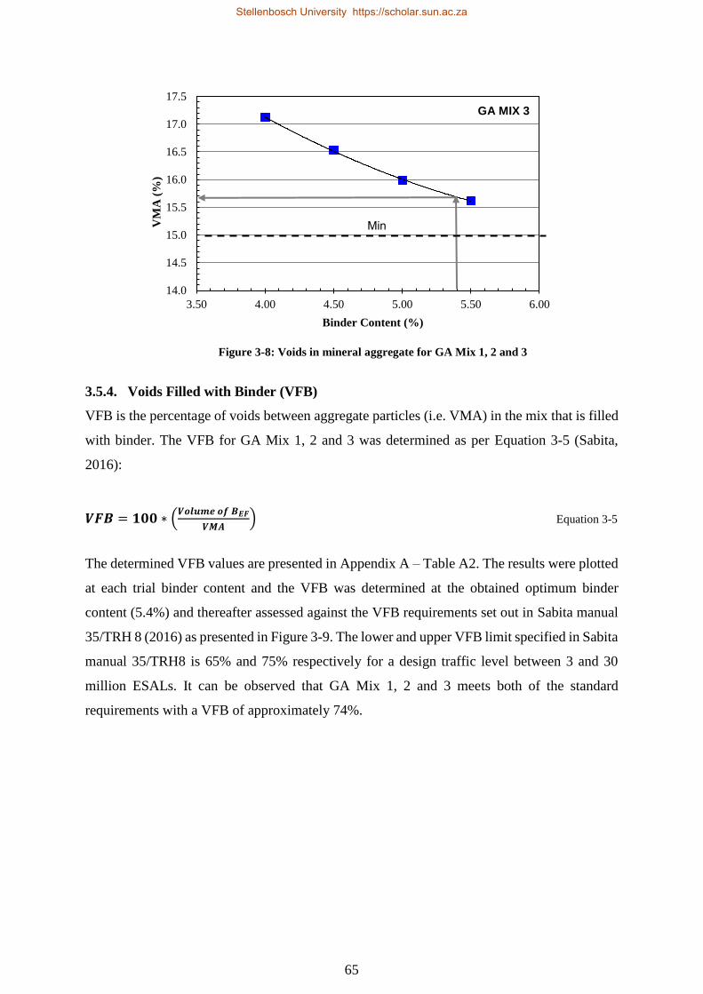
Figure 3-8: Voids in mineral aggregate for GA Mix 1, 2 and 3 .............................................. 65
Figure 3-9: Voids filled with binder for GA Mix 1, 2 and 3 ................................................... 66
Figure 3-10: Sand equivalency of fine granite aggregates and recycled crushed glass ........... 71
Figure 3-11: Fine angular crushed glass particles (Scale: 200 µm, Mag: 20x) ...................... 73
Stellenbosch University https://scholar.sun.ac.za
Page 15
xiv
Figure 3-12: Textured features on surface of fine crushed glass particles .............................. 74
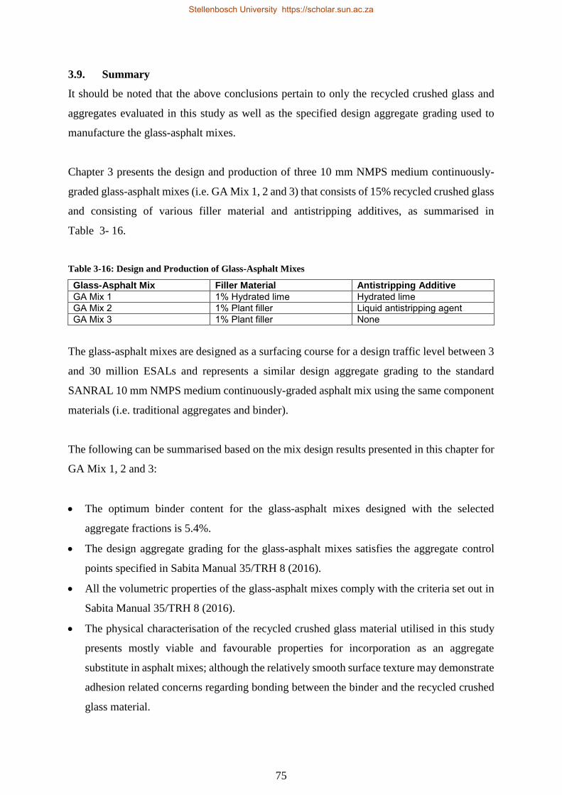
Figure 3-13: SEM of a) glass-asphalt mix and b) conventional asphalt mix .......................... 74
Figure 4-1: Modified Lottman testing as per ASTM D4867M................................................ 78
Figure 4-2: Average ITS results for GA Mix 1, 2 and 3 .......................................................... 80
Figure 4-3: TSR results for GA Mix 1, 2 and 3 ....................................................................... 81
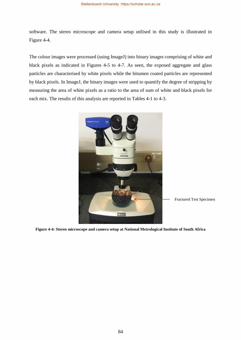
Figure 4-4: Stereo microscope and camera setup .................................................................... 84
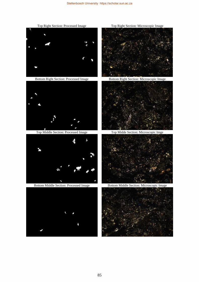
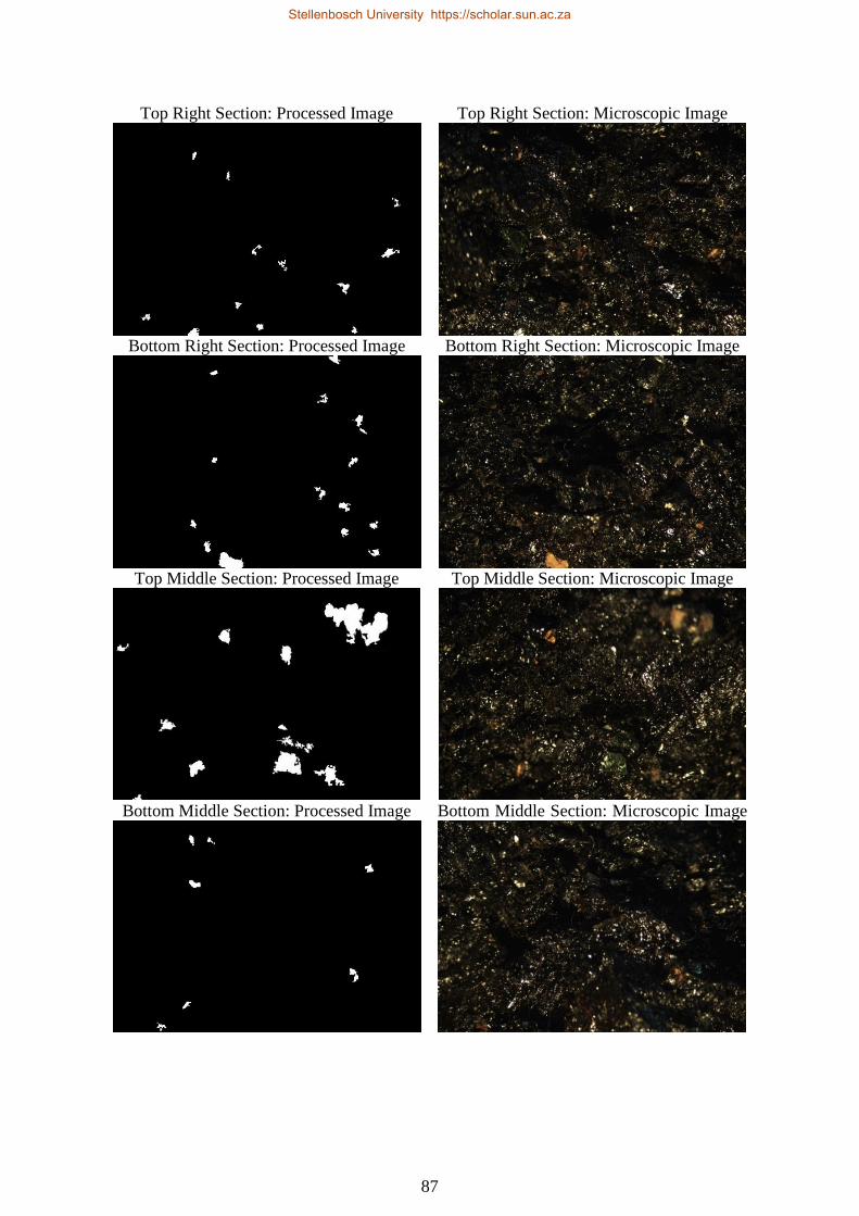
Figure 4-5: Microscopic analysis of GA Mix 1 after Modified Lottman test .......................... 86
Figure 4-6: Microscopic analysis of GA Mix 2 after Modified Lottman test .......................... 88
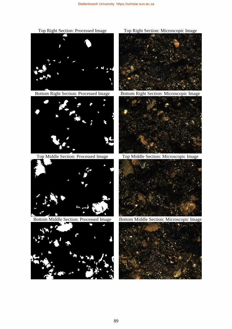
Figure 4-7: Microscopic analysis of GA Mix 3 after Modified Lottman test .......................... 90
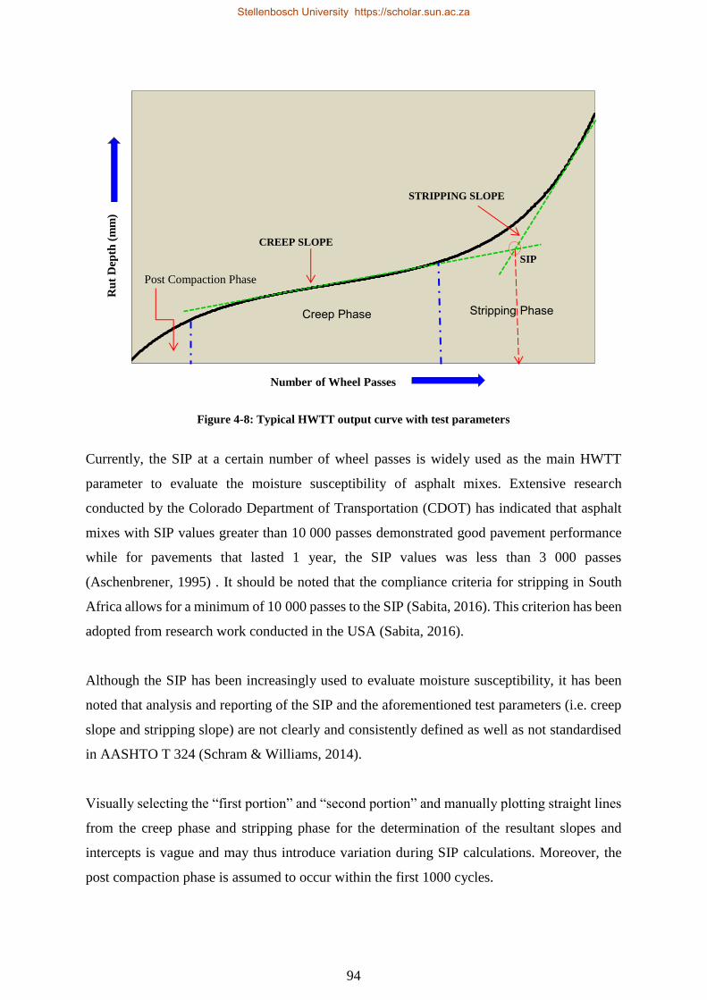
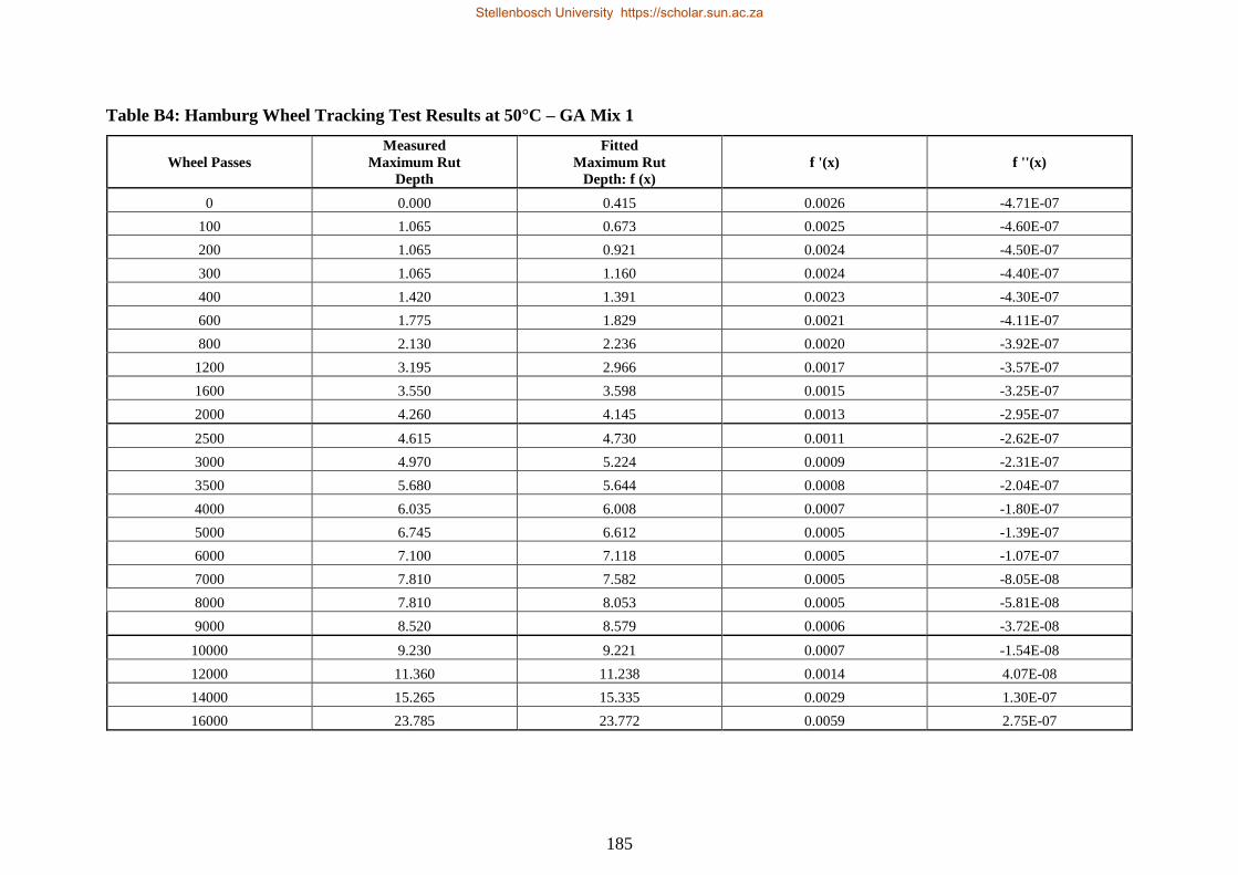
Figure 4-8: Typical HWTT output curve with test parameters................................................ 94
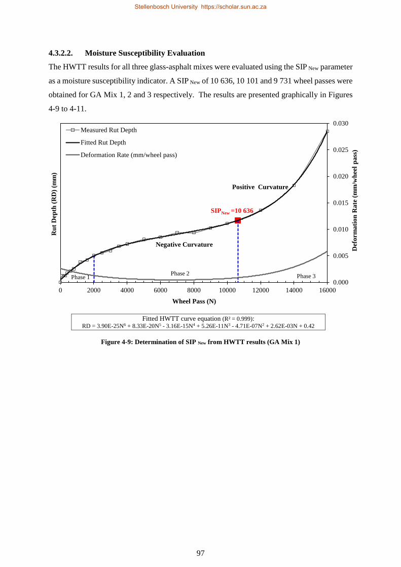
Figure 4-9: Determination of SIP New from HWTT results (GA Mix 1) ................................. 97
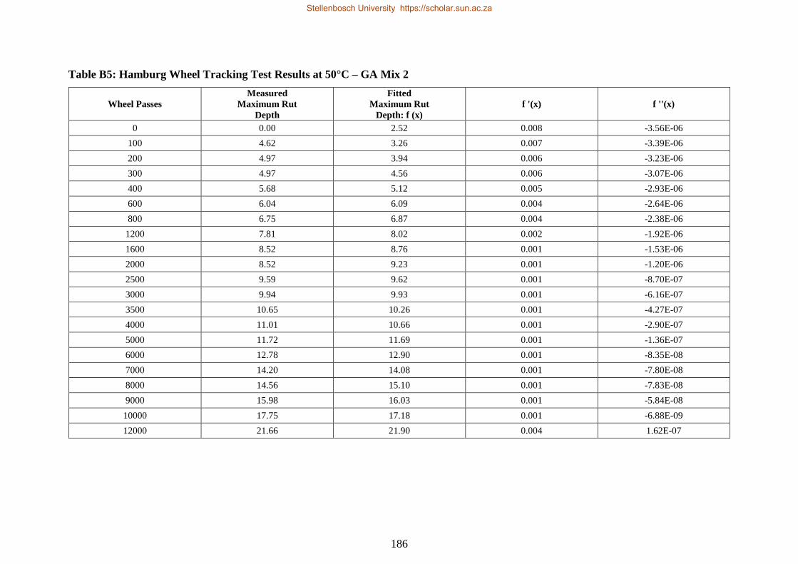
Figure 4-10: Determination of SIP New from HWTT results (GA Mix 2) ............................... 98
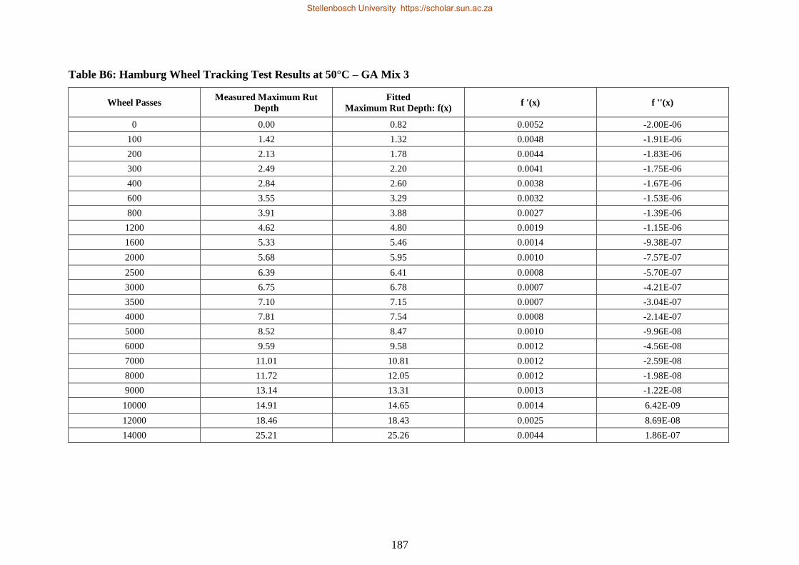
Figure 4-11: Determination of SIP New from HWTT results (GA Mix 3) ............................... 98
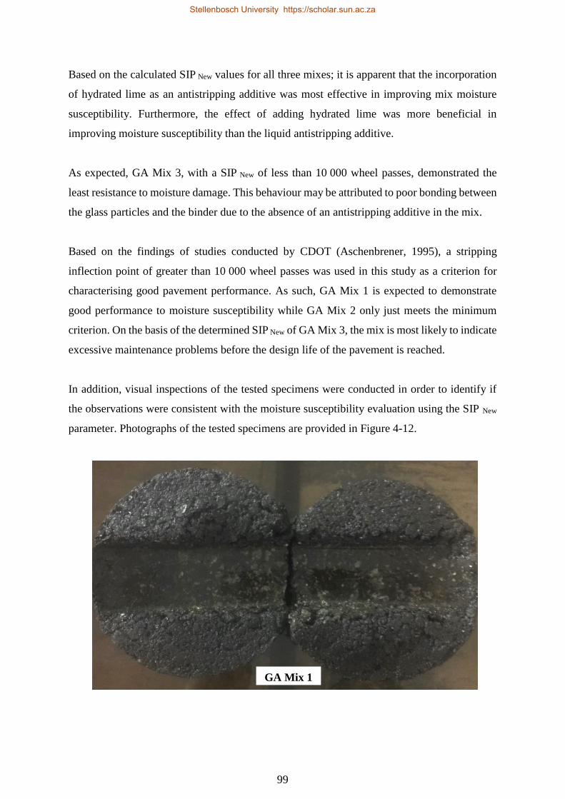
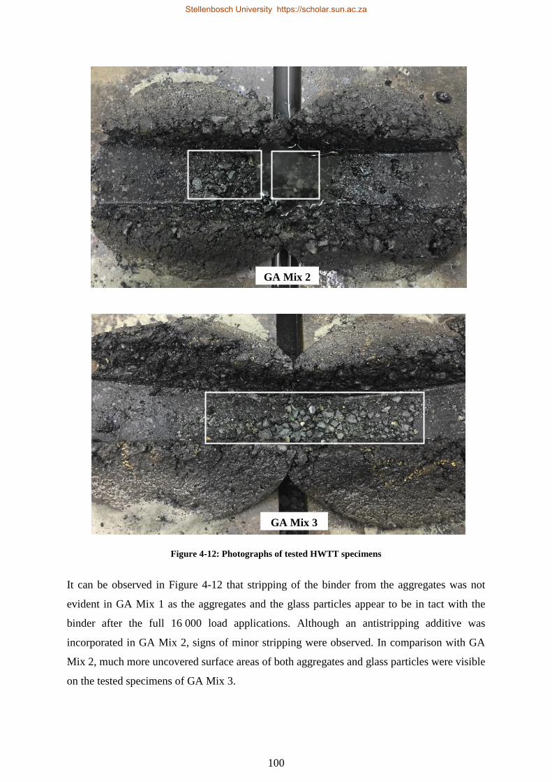
Figure 4-12: Photographs of tested HWTT specimens .......................................................... 100
Figure 4-13: Determination of SIP Current from HWTT results (GA Mix 1) .......................... 102
Figure 4-14: Determination of SIP Current from HWTT results (GA Mix 2) .......................... 102
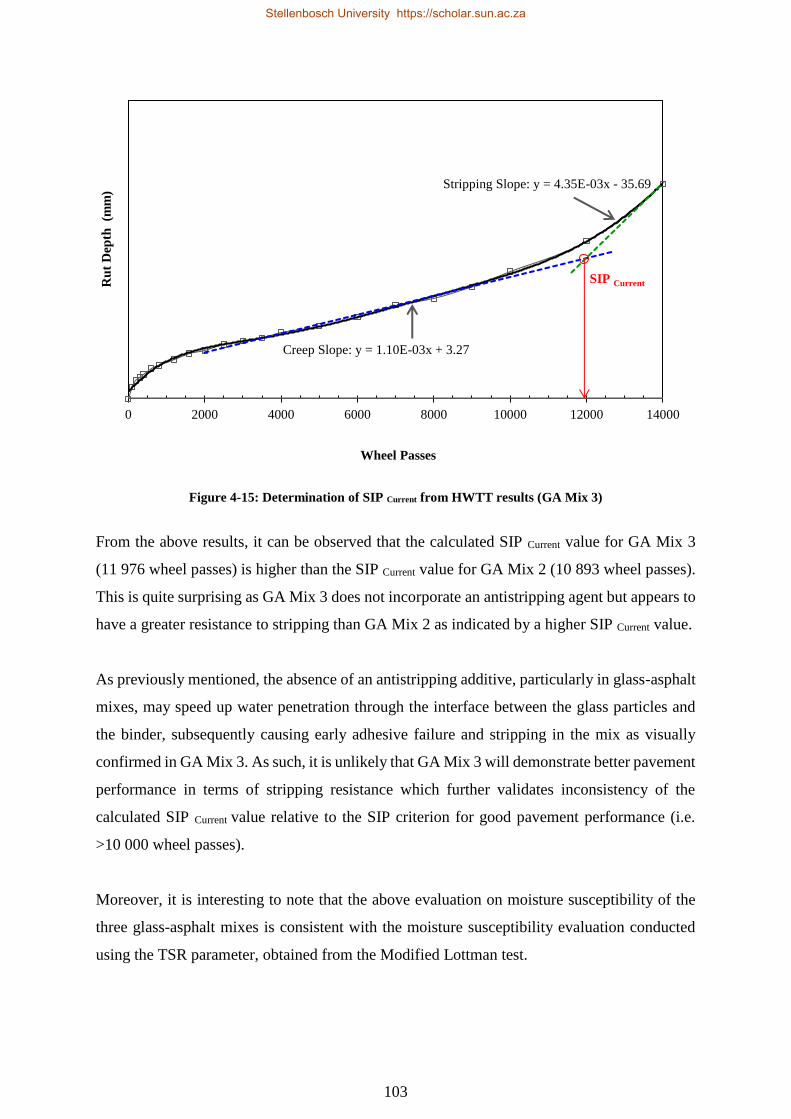
Figure 4-15: Determination of SIP Current from HWTT results (GA Mix 3) .......................... 103
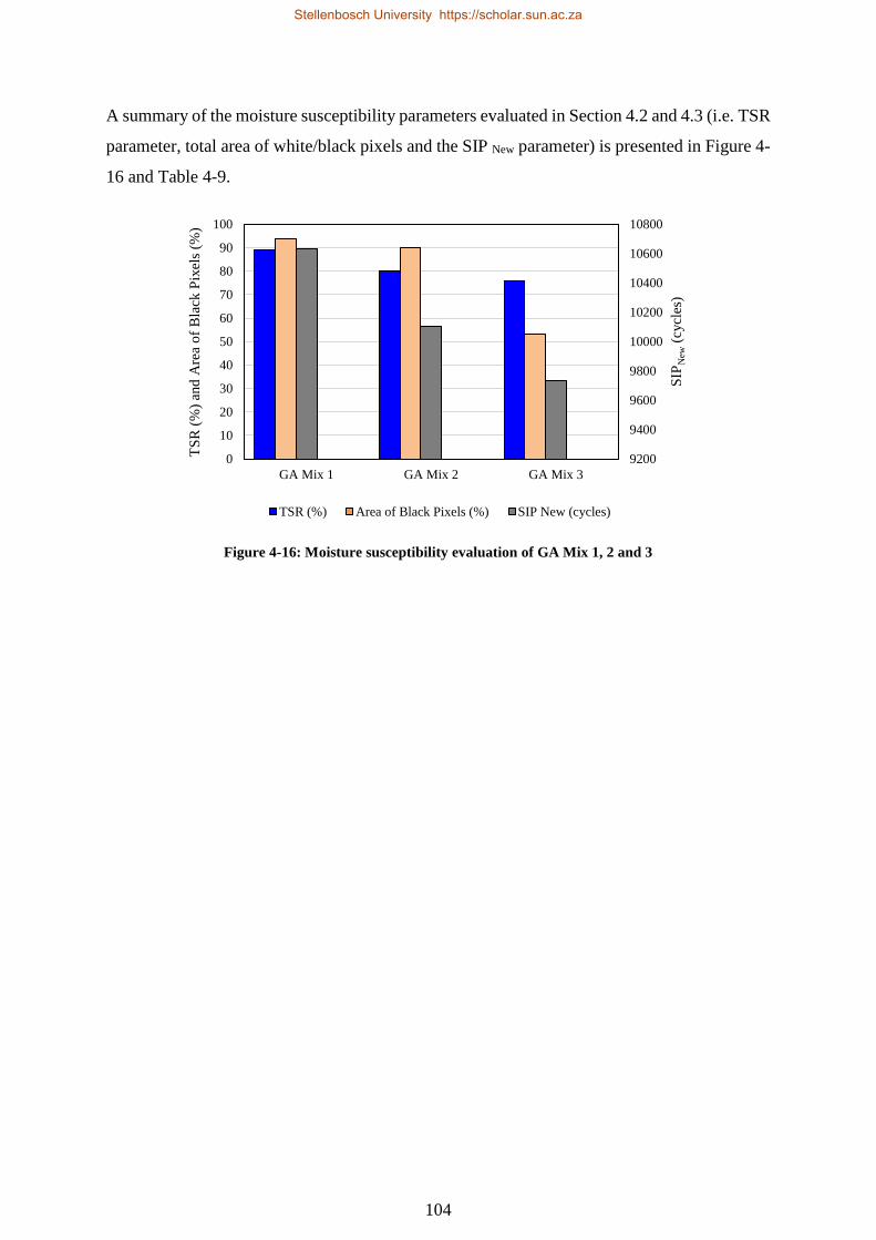
Figure 4-16: Moisture susceptibility evaluation of GA Mix 1, 2 and 3 ................................. 104
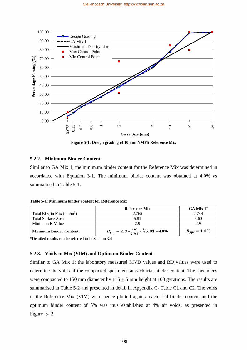
Figure 5-1: Design grading of 10 mm NMPS Reference Mix ............................................... 108
Figure 5-2: Bulk density and voids and in Reference Mix .................................................... 109
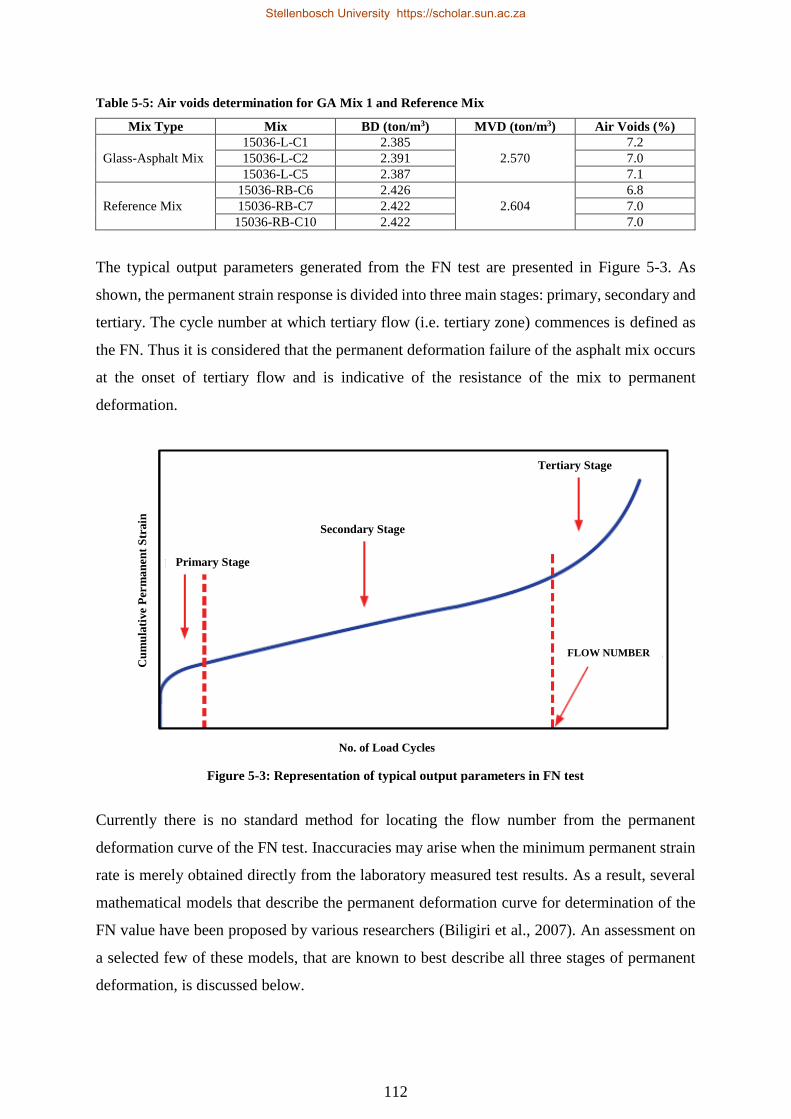
Figure 5-3: Representation of typical output parameters in FN test ...................................... 112
Figure 5-4: Power model describing permanent deformation of GA Mix 1.......................... 114
Figure 5-5: Power model describing permanent deformation of Reference Mix .................. 114
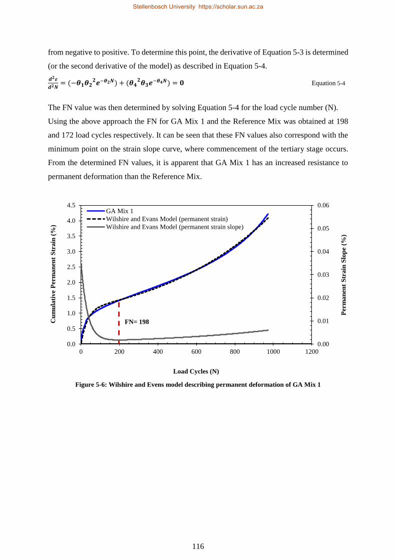
Figure 5-6: Wilshire and Evens model of GA Mix 1............................................................. 116
Figure 5-7: Wilshire and Evens model of Reference Mix ..................................................... 117
Figure 5-8: Measured vs predicted permanent deformation of GA Mix 1 ............................ 117
Figure 5-9: Measured vs predicted permanent deformation of Reference Mix ..................... 118
Figure 5-10: Polynomial model describing permanent deformation of GA Mix 1 ............... 119
Figure 5-11: Polynomial model describing permanent deformation of Reference Mix ........ 120
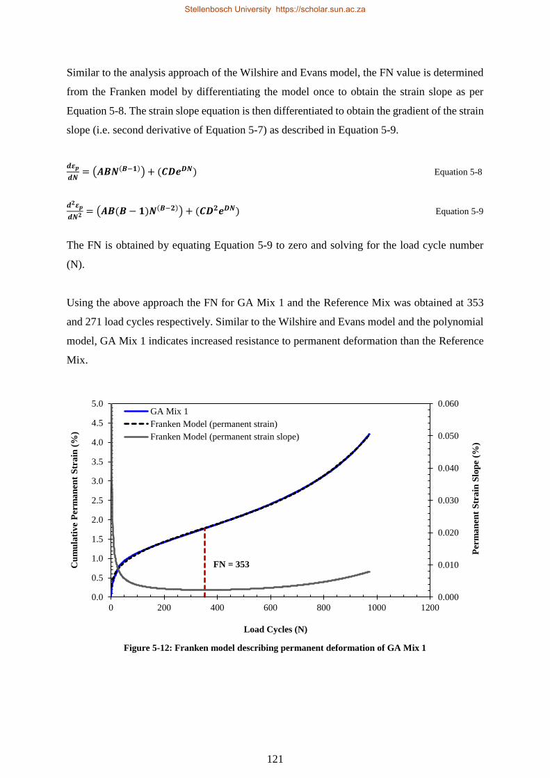
Figure 5-12: Franken model describing permanent deformation of GA Mix 1 ..................... 121
Figure 5-13: Franken model describing permanent deformation of Reference Mix ............. 122
Figure 5-14: Measured vs predicted permanent deformation of GA Mix 1 .......................... 122
Figure 5-15: Measured vs predicted permanent deformation of Reference Mix ................... 123
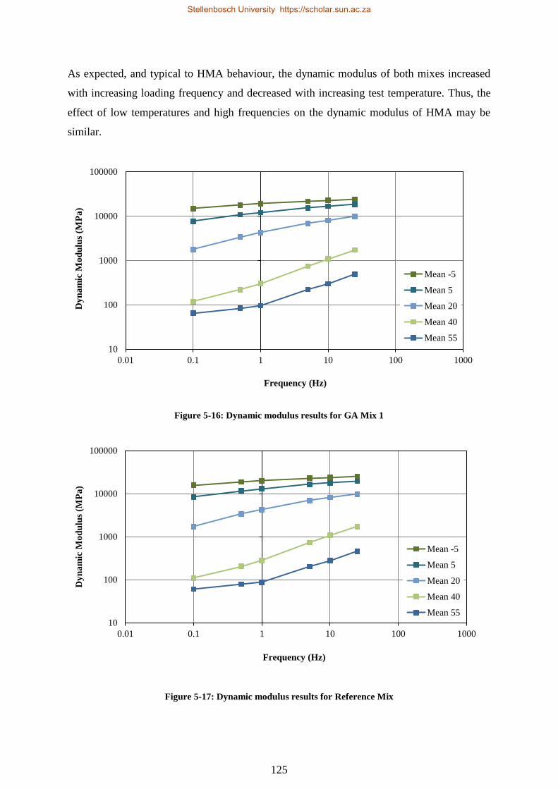
Figure 5-16: Dynamic modulus results for GA Mix 1 ........................................................... 125
Stellenbosch University https://scholar.sun.ac.za
Page 16
xv
Figure 5-17: Dynamic modulus results for Reference Mix ................................................... 125
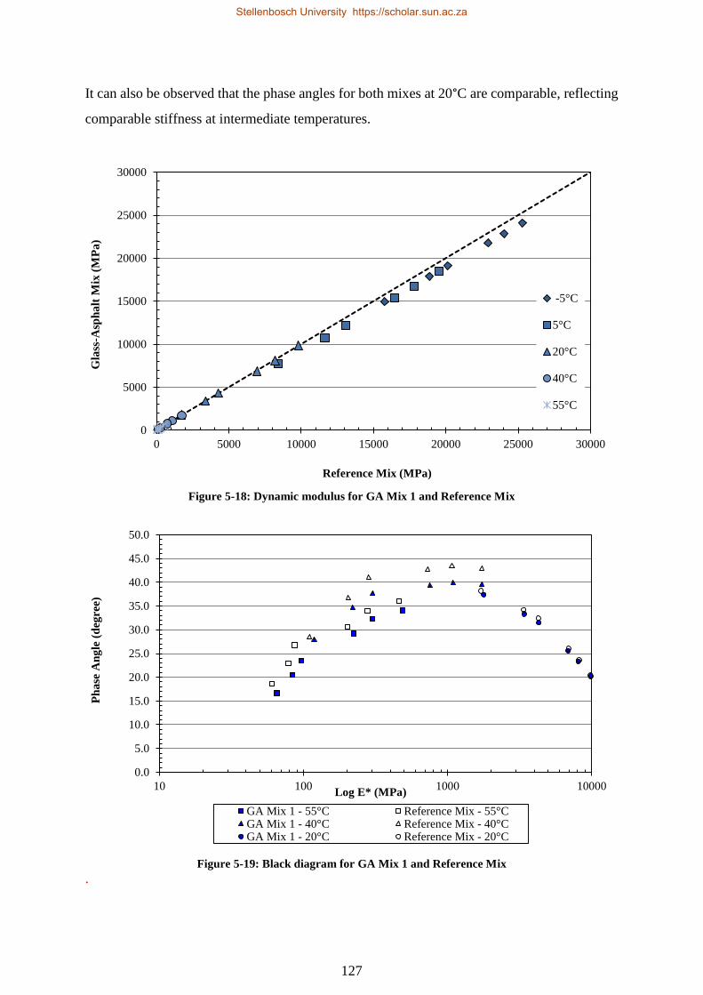
Figure 5-18: Dynamic modulus for GA Mix 1 and Reference Mix ...................................... 127
Figure 5-19: Black diagram for GA Mix 1 and Reference Mix ............................................ 127
Figure 5-20: Applied stress and strain response .................................................................... 131
Figure 5-21: Complex modulus components ......................................................................... 132
Figure 5-22: Viscosity-temperature relationship for RTFO 50/70 penetration-grade binder 137
Figure 5-23: Representation of Burger’s model .................................................................... 138
Figure 5-24: Representation of Huet-Sayegh model ............................................................. 139
Figure 5-25: Sigmoidal model master curves of GA Mix 1 and Reference Mix at 20°C ..... 140
Figure 5-26: Measured versus predicted dynamic modulus for GA Mix 1 ........................... 141
Figure 5-27: Burger’s model representation of Cole-Cole diagram for GA Mix 1 ............... 142
Figure 5-28: Burger’s model representation of Black diagram for GA Mix 1 ...................... 143
Figure 5-29: Master curves of GA Mix 1 at 20°C ................................................................ 143
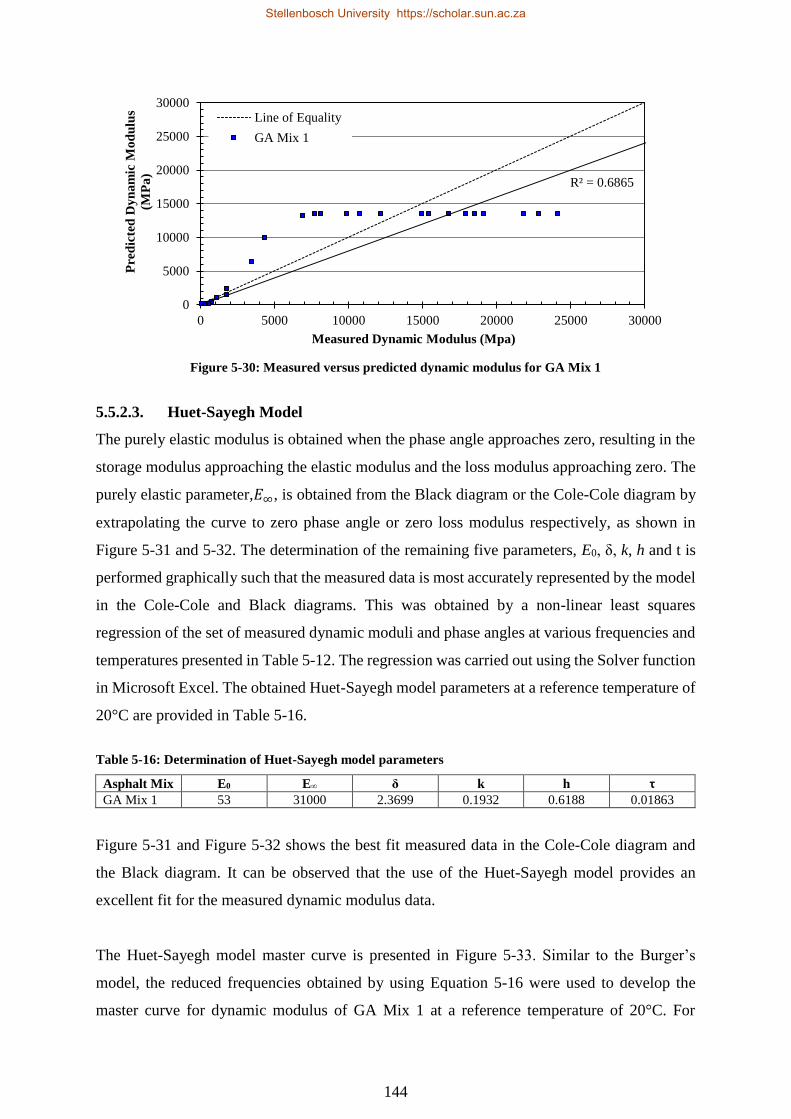
Figure 5-30: Measured versus predicted dynamic modulus for GA Mix 1 ........................... 144
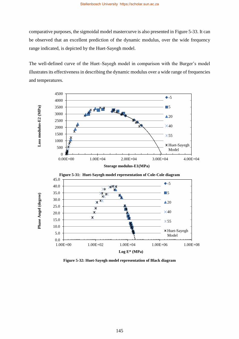
Figure 5-31: Huet-Sayegh model representation of Cole-Cole diagram .............................. 145
Figure 5-32: Huet-Sayegh model representation of Black diagram ...................................... 145
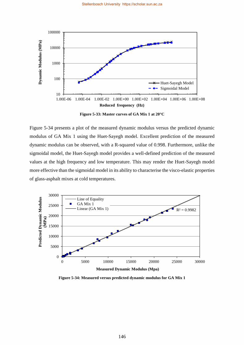
Figure 5-33: Master curves of GA Mix 1 at 20°C ................................................................. 146
Figure 5-34: Measured versus predicted dynamic modulus for GA Mix 1 ........................... 146
Figure 6-1: Pavement Structure 1 (a) and Pavement Structure 2 (b) ..................................... 149
Figure 6-2: Vertical and horizontal stresses in Pavement 1 ................................................... 153
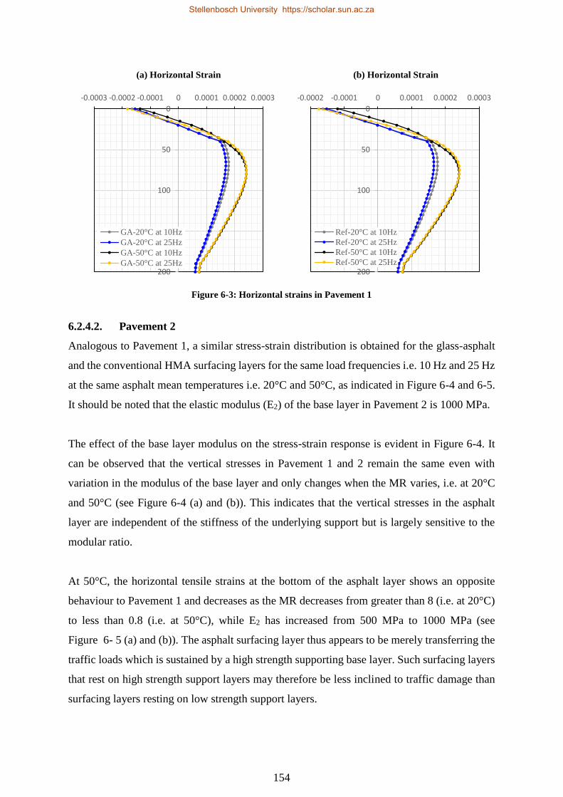
Figure 6-3: Horizontal strains in Pavement 1 ........................................................................ 154
Figure 6-4: Vertical and horizontal stresses in Pavement 2 ................................................... 155
Figure 6-5: Horizontal strains in Pavement 2 ........................................................................ 156
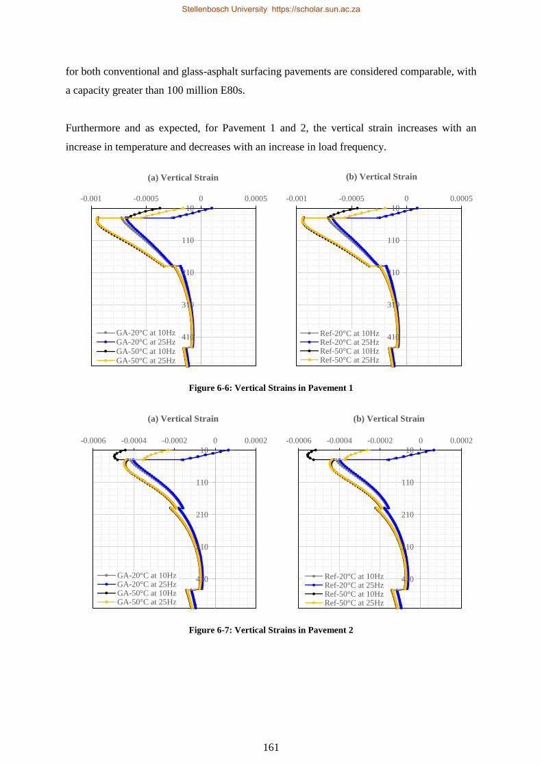
Figure 6-6: Vertical Strains in Pavement 1 ............................................................................ 161
Figure 6-7: Vertical Strains in Pavement 2 ............................................................................ 161
Stellenbosch University https://scholar.sun.ac.za
Page 17
1
1. INTRODUCTION
1.1 Background
The National Environmental Management: Waste Act (Act 59 of 2008) commits National
Government to, amongst others, promote “waste minimisation, reuse, recycling and recovery
of waste” in South Africa. However, national waste information obtained in 2011 indicates that
an estimated 70% (approx. 650,000 tonnes) of waste glass generated in South Africa was
landfilled, while only 30% was recycled. This data highlights that a substantial amount of waste
glass could, therefore, potentially be diverted from landfill and recovered to be recycled or
reused.
Additionally, considerable quantities of recycled crushed glass fines (less than 5 mm),
accumulate as stockpiles at glass packaging manufacturing plants in Gauteng and the Western
Cape provinces of South Africa. These processed glass fines, which are unusable in the glass
packaging manufacturing process, are stockpiled and earmarked for disposal to landfill;
thereby contributing to the waste glass that is currently being landfilled. This further adds
undue pressure on rapidly depleting landfill airspace and has led to the necessity for adopting
sustainable practices. Waste glass that is recovered to be recycled or re-used is a key component
in this.
The pavement industry, amongst others, can provide a number of alternative uses for this
recovered waste glass. One such use is where crushed waste glass can be used as a material
substitute in asphalt pavements, which will provide a more cost effective and environmentally
friendly solution to disposal and will add value to this otherwise waste material.
The use of crushed glass in Hot Mix Asphalt (HMA) paving applications has been widely
implemented in the United States and Canada since the early 1970’s. Other countries that have
reported using crushed glass in asphalt paving applications include United Kingdom, Australia,
New Zeland, Japan and Taiwan (Yamanaka et al., 2001; Su & Chen, 2002; Dane County
Department of Public Works, 2003; Arnold et al., 2008; Australian government Department of
Sustainability, Environment, Water Population and Communities, 2011; Andela & Sorge,
n.d.).
Stellenbosch University https://scholar.sun.ac.za
Page 18
2
Early applications of crushed glass in asphalt pavements in the United States incorporated glass
particles greater than 12.5 mm with quantities in excess of 25%. The application of coarse glass
particles (> 5 mm) in large quantities was considered to be a major contributing factor to the
stripping and ravelling problems reported in early glass-asphalt pavement applications.
More recently, 10 to 15% crushed glass has been specified for use in asphalt wearing courses
in the United States; while some countries, e.g. New Zealand, utilise as little as 5% glass
content in asphalt base courses. Various studies have shown that improved performance, in
terms of permanent deformation, has been obtained for HMA pavements incorporating up to
15% crushed glass using both fine and coarse graded glass particles with a maximum particle
size of up to 9.5 mm. Furthermore, recommendations on the inclusion of antistripping additives
and their relevance in resisting moisture induced damage in glass-asphalt mixes have been
based specifically on the grading of the glass particles utilised in combination with specific
types of coarse and fine aggregates common to a particular region or country.
In South Africa, however, minimal research has been conducted on the viability of using
recycled crushed glass in asphalt pavement applications. Research is, therefore, needed to
characterise the performance of locally available recycled crushed glass in asphalt pavements
in South Africa. In this regard, the interaction of the glass particles in combination with
conventional materials typically used for asphalt production in South Africa, and its effect on
asphalt mix performance, requires investigation.
Investigations in this regard will contribute towards developing innovations to address “waste
minimisation, re-use, recycling and recovery of waste”, whilst simultaneously developing
solutions to maintain or otherwise improve the performance of asphalt pavements in South
Africa. In addition, recycling waste glass for use as a secondary material in pavement
applications will contribute towards stimulating a regional secondary resources economy with
potential for industrial development and creation of sustainable jobs.
Stellenbosch University https://scholar.sun.ac.za
Page 19
3
1.2 Problem Statement
There is currently a gap in existing knowledge on the engineering performance of recycled
crushed glass in South African asphalt mixes. Nominal research has been conducted in South
Africa on the suitability of locally available recycled crushed glass as a substitute for asphalt
aggregates currently used and the associated engineering performance properties of asphalt
mixes incorporating recycled crushed glass.
Furthermore, current entrenched asphalt mix design methods and specifications in South Africa
have limited the use of alternative material design practices resulting in the use of expensive
materials, e.g. highly modified bituminous binder, to achieve the required pavement
performance. In many cases, such materials are specified too easily before exploring other
pioneering material design alternatives.
Therefore, there is a need to investigate the effectiveness of recycled crushed glass as a
substitute material in South African asphalt mixes that will maintain or otherwise improve
pavement performance. The findings of the investigation can further be documented as
guidelines and incorporated into future mix design methods and specifications for South
Africa.
1.3 Research Goal and Objectives
1.3.1. Research Goal
The goal of this study is to determine the influence of recycled crushed glass on the engineering
performance of a continuously-graded asphalt wearing course mix.
1.3.2. Research Objectives
To achieve the research goal, the following objectives were developed:
Mix design and production of a medium continuously-graded asphalt wearing course mix
consisting of 15% recycled crushed glass.
Evaluate the stripping potential of the glass-asphalt mix with and without the use of local
anti-stripping additives.
Compare the stiffness and deformation properties of the glass-asphalt mix and a traditional
asphalt wearing course mix commonly used for road construction in South Africa.
Stellenbosch University https://scholar.sun.ac.za
Page 20
4
Characterise the deformation and linear visco-elastic behaviour of the glass-asphalt mix
using selected mathematical models.
1.4 Research Scope
The scope of this study includes the following:
Review of available literature on the utilisation of crushed glass in HMA.
Conduct survey to identify possible sources of crushed waste glass in South Africa.
Procurement of constituent materials for glass-asphalt mix design and production.
Development (design and production) of glass-asphalt mix.
Conduct series of laboratory tests to determine the physical and engineering properties of
glass-asphalt mix.
Data processing and analysis of laboratory test results for performance evaluation and
comparison.
1.5 Outline of Dissertation
This dissertation is presented as follows:
Chapter 1 provides the background and need for the study and highlights the objectives and
scope of the study undertaken.
Chapter 2 provides a literature review on studies conducted on the utilisation of crushed glass
in HMA and its effect on the laboratory as well as in-situ performance properties of glass-
asphalt mixes. An overview on the global utilisation of crushed glass in asphalt pavement
applications is also provided.
Chapter 3 presents the design and production of a continuously-graded glass-asphalt mix and
discusses the volumetric properties of the mix in relation with criteria set out for traditional
continuously-graded asphalt mixes in South Africa. A review on the physical characteristics of
the locally available recycled crushed glass material is also presented.
Chapter 4 presents the selection of the optimum glass-asphalt mix based on an evaluation on
the degree of moisture susceptibility of the mix with and without the addition of selected
Stellenbosch University https://scholar.sun.ac.za
Page 21
5
antistripping additives. The moisture damage evaluation is discussed relative to South African
standard requirements.
Chapter 5 presents a comparison of the stiffness and permanent deformation properties of the
glass-asphalt mix and a traditional asphalt mix. Furthermore, an evaluation on the use of
selected constitutive models namely, Kelvin, Burger’s and Huet-Sayegh to effectively
characterise the linear visco-elastic behaviour of the glass-asphalt mix over a wide range of
temperatures and loading frequencies is presented. Similarly, the use of selected mathematical
models namely, power model, Wilshire and Evans model, polynomial model and Francken
model, to effectively evaluate the permanent deformation behaviour of the glass-asphalt mix is
presented.
Chapter 6 presents a multi-layer linear-elastic analysis of the glass-asphalt surfacing layer
within a typical pavement structure of ES10 and ES30 design structural capacity. The effects
of temperature and loading frequency variation on the stress-strain behaviour as well as the
structural capacity of the glass-asphalt surfacing layer overlying a high and low strength
supporting base layer is assessed.
Chapter 7 provides the conclusions and recommendations of the study.
Stellenbosch University https://scholar.sun.ac.za
Page 22
6
2. LITERATURE STUDY
2.1 Introduction
2.1.1 Domestic Waste Glass
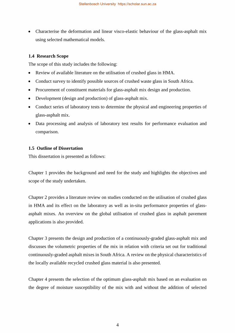
According to the National Waste Information Baseline Report (Department of Environmental
Affairs, 2012), more than 900,000 tonnes of domestic waste glass is assessed to have been
produced in South Africa in 2011. This comprises of approximately 4% of the general waste
stream in South Africa for the 2011 year (Department of Environmental Affairs, 2012). See
Figure 2-1. Of this waste, approximately 30% was recycled and the remaining 70% disposed
at landfill (Department of Environmental Affairs, 2012). A substantial amount of domestic
waste glass could, therefore, potentially be diverted from landfill and recovered to be recycled
or reused.
Figure 2-1: General waste composition, 2011 (percentage by mass)
(Department of Environmental Affairs, 2012)
34%
21%
14%
13%
7%6% 4%
1%
Non-recyclable Municipal
Waste
Construction and Demolition
Waste
Metal Waste
Organic Waste
Paper
Plastic
Glass
Tyres
Stellenbosch University https://scholar.sun.ac.za
Page 23
7
2.1.2 Domestic Waste Glass Management in South Africa
The legislative framework for waste management in South Africa stems from Section 24 of the
Constitution, which commits “to secure an environment that is not harmful to the health and
well-being of the people of South Africa” (Department of Environmental Affairs, 2012). The
legislation which has been promulgated through Parliament to establish and promote this is the
National Environmental Management Act (No. 107 of 1998) (NEMA) and the National
Environmental Management: Waste Act (No. 59 of 2008) (NEM: WA).
The NEM: WA establishes, amongst others, the following objectives with regards to waste
management in South Africa (Department of Environmental Affairs, 2012):
• “Minimise the consumption of natural resources,
• Avoid and minimise the generation of waste,
• Reduce, re-use, recycle and recover waste”.
Furthermore, the NEMA and NEM: WA have led to the development of the National Waste
Management Strategy (NWMS) (2011), which directs local municipalities to develop
alternative waste management processes, as one of their main objectives, to ensure diversion
of waste sent to landfills (Department of Environmental Affairs, 2012).
A few municipalities have begun to address this objective by promoting separation of waste at
source initiatives, which makes use of different waste collection bags for general waste and
recyclable waste, which can then be collected for recycling. One of the leaders in implementing
this initiative is the Ethekwini municipality in KwaZulu Natal, who to date have 1 million
homes involved and contributing to the initiative, and hence seem well established for
improving their waste glass collection figures.
In spite of the fact that recycling is enacted within South Africa, most recycling exercises are
generally determined by the industry through the foundation of industry bodies or Producer
Responsibility Organisations (PRO). PRO’s are non-profit organisations supported by the
industry to advance the recovery and recycling of waste materials in South Africa.
One such PRO is The Glass Recycling Company (TGRC), which is responsible for promoting
/ supporting and enabling the recovery and recycling of waste glass. The TGRC is supported
by the Department of Environmental Affairs, and since its establishment in 2006, South Africa
Stellenbosch University https://scholar.sun.ac.za
Page 24
8
has seen a considerable increase in the recycling rate of glass packaging, which has increased
from just 18% in 2005/06 to 41.1% in 2015/16.
Some of the initiatives implemented by the TGRC include the installation of over 2000 glass
banks, which are placed in various locations in communities and are intended for members of
the public to have easy access to waste glass deposit points where glass can be deposited for
recycling. The TGRC also provides an SMS service for members of the public who are
interested in finding their nearest glass bank.
Another initiative by the TGRC allows members of the public, who are mostly from previously
disadvantaged backgrounds, to establish buy-back centres, where glass can be collected for
recycling. Equipment to establish such centres is provided by the TGRC and the buy-back
centres in turn provide a source of income to jobless members of the public who form the
majority of waste glass collectors.
In addition to the initiatives mentioned, South Africa has also established a glass returnable
deposit system, which is a large scale initiative and sees a mandatory deposit fee being charged
on consumers who purchase returnable glass bottles. This fee is reimbursed to consumers upon
return of the bottles to retail outlets, and the retailers in turn send the returned bottles back to
the bottle supplier, who may then clean and re-use or recycle the returned bottles.
Notwithstanding the objectives from the NEM: WA as well as recycling initiatives undertaken
by industry bodies, the shortage of landfill airspace as well the ever increasing cost of raw
materials warrants development and expansion of the recycling industry in South Africa.
Furthermore the various green economy policies and strategies also have a positive spin off on
job creation within the country.
2.1.3 Sources of Recycled Crushed Glass in South Africa
A survey of the major consumers in the waste glass market in South Africa was conducted
during the course of this study. At present there is only one well established market for
recovered domestic waste glass in the country; which is the glass packaging industry. The
survey population thus included two leading glass packaging manufacturing companies as well
as other major collectors of domestic waste glass.
Stellenbosch University https://scholar.sun.ac.za
Page 25
9
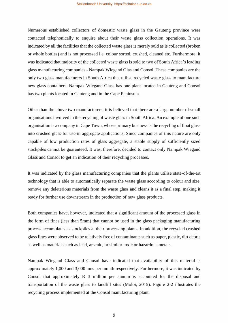
Numerous established collectors of domestic waste glass in the Gauteng province were
contacted telephonically to enquire about their waste glass collection operations. It was
indicated by all the facilities that the collected waste glass is merely sold as is collected (broken
or whole bottles) and is not processed i.e. colour sorted, crushed, cleaned etc. Furthermore, it
was indicated that majority of the collected waste glass is sold to two of South Africa’s leading
glass manufacturing companies - Nampak Wiegand Glas and Consol. These companies are the
only two glass manufacturers in South Africa that utilise recycled waste glass to manufacture
new glass containers. Nampak Wiegand Glass has one plant located in Gauteng and Consol
has two plants located in Gauteng and in the Cape Peninsula.
Other than the above two manufacturers, it is believed that there are a large number of small
organisations involved in the recycling of waste glass in South Africa. An example of one such
organisation is a company in Cape Town, whose primary business is the recycling of float glass
into crushed glass for use in aggregate applications. Since companies of this nature are only
capable of low production rates of glass aggregate, a stable supply of sufficiently sized
stockpiles cannot be guaranteed. It was, therefore, decided to contact only Nampak Wiegand
Glass and Consol to get an indication of their recycling processes.
It was indicated by the glass manufacturing companies that the plants utilise state-of-the-art
technology that is able to automatically separate the waste glass according to colour and size,
remove any deleterious materials from the waste glass and cleans it as a final step, making it
ready for further use downstream in the production of new glass products.
Both companies have, however, indicated that a significant amount of the processed glass in
the form of fines (less than 5mm) that cannot be used in the glass packaging manufacturing
process accumulates as stockpiles at their processing plants. In addition, the recycled crushed
glass fines were observed to be relatively free of contaminants such as paper, plastic, dirt debris
as well as materials such as lead, arsenic, or similar toxic or hazardous metals.
Nampak Wiegand Glass and Consol have indicated that availability of this material is
approximately 1,000 and 3,000 tons per month respectively. Furthermore, it was indicated by
Consol that approximately R 3 million per annum is accounted for the disposal and
transportation of the waste glass to landfill sites (Moloi, 2015). Figure 2-2 illustrates the
recycling process implemented at the Consol manufacturing plant.
Stellenbosch University https://scholar.sun.ac.za
Page 26
10
An alternative application can be proposed whereby the waste glass can be used as an aggregate
substitution in pavement construction which will provide a more cost effective and
environmentally friendly solution to disposal. The possibility of using waste glass in pavement
applications can be seen a sustainable alternative to natural aggregates, especially since good
quality aggregates are scarce and glass cullet (crushed glass) as a raw material has no associated
financial costs currently in South Africa.
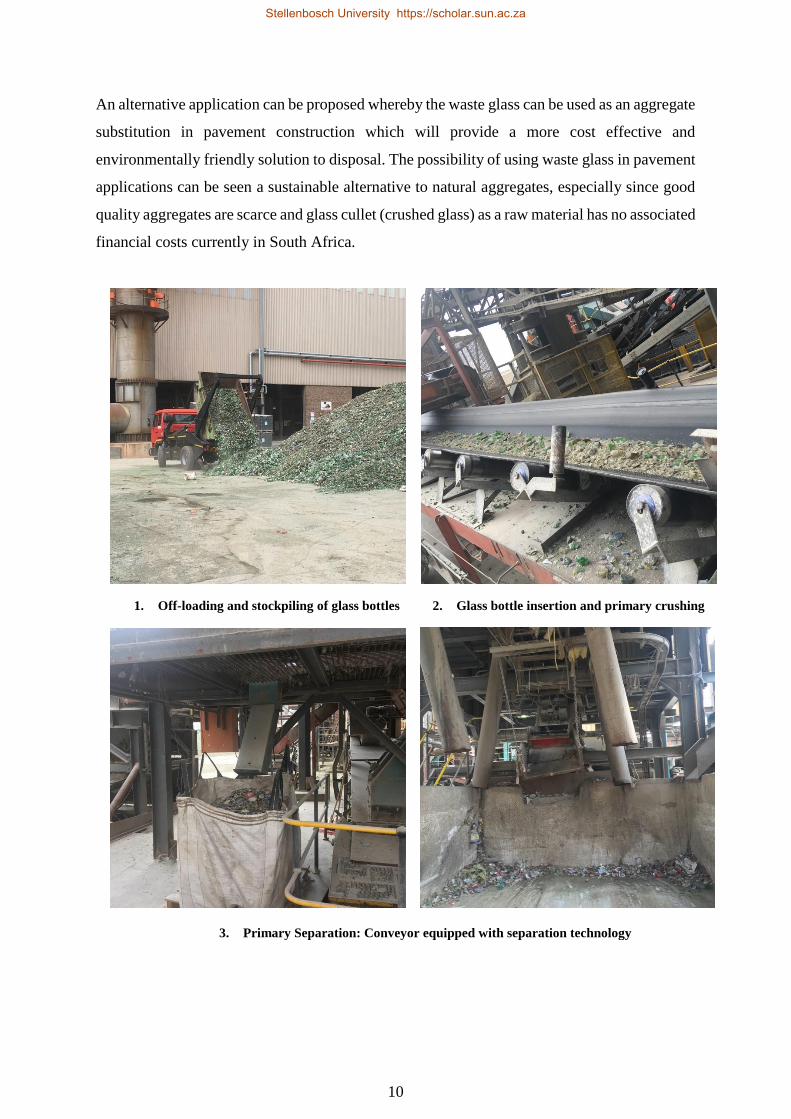
1. Off-loading and stockpiling of glass bottles
2. Glass bottle insertion and primary crushing
3. Primary Separation: Conveyor equipped with separation technology
Stellenbosch University https://scholar.sun.ac.za
Page 27
11
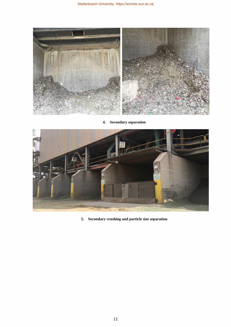
4. Secondary separation
5. Secondary crushing and particle size separation
Stellenbosch University https://scholar.sun.ac.za
Page 28
12
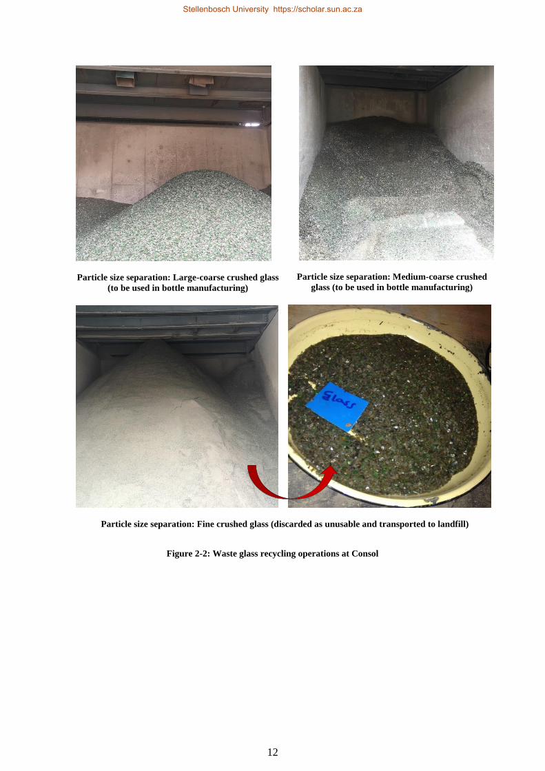
Particle size separation: Large-coarse crushed glass
(to be used in bottle manufacturing)
Particle size separation: Medium-coarse crushed
glass (to be used in bottle manufacturing)
Particle size separation: Fine crushed glass (discarded as unusable and transported to landfill)
Figure 2-2: Waste glass recycling operations at Consol
Stellenbosch University https://scholar.sun.ac.za
Page 29
13
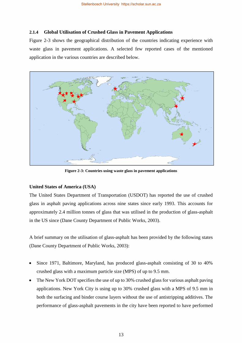
2.1.4 Global Utilisation of Crushed Glass in Pavement Applications
Figure 2-3 shows the geographical distribution of the countries indicating experience with
waste glass in pavement applications. A selected few reported cases of the mentioned
application in the various countries are described below.
Figure 2-3: Countries using waste glass in pavement applications
United States of America (USA)
The United States Department of Transportation (USDOT) has reported the use of crushed
glass in asphalt paving applications across nine states since early 1993. This accounts for
approximately 2.4 million tonnes of glass that was utilised in the production of glass-asphalt
in the US since (Dane County Department of Public Works, 2003).
A brief summary on the utilisation of glass-asphalt has been provided by the following states
(Dane County Department of Public Works, 2003):
Since 1971, Baltimore, Maryland, has produced glass-asphalt consisting of 30 to 40%
crushed glass with a maximum particle size (MPS) of up to 9.5 mm.
The New York DOT specifies the use of up to 30% crushed glass for various asphalt paving
applications. New York City is using up to 30% crushed glass with a MPS of 9.5 mm in
both the surfacing and binder course layers without the use of antistripping additives. The
performance of glass-asphalt pavements in the city have been reported to have performed
Stellenbosch University https://scholar.sun.ac.za
Page 30
14
"as well as, if not better than, conventional pavements." Brooklyn is utilising 10% recycled
crushed glass (obtained from a glass recycling facility) in asphalt surfacing layers. Since
1994, Brooklyn, New York, has reported the use of crushed glass in asphalt paving
applications for more than six years.
Pennsylvania has utilised approximately 100,000 tonnes of crushed glass as an aggregate
substitute in asphalt in 1992.
Menasha, Wisconsin, has utilised crushed glass bottles in the production of glass-asphalt
with a glass replacement ratio of 10%. In 1992, a glass-asphalt pavement incorporating
7.5% crushed glass with a MPS of 9.5 mm was constructed. The addition of an antistripping
additive was also used. Following a year post construction no moisture damage or skid
related concerns were reported. Furthermore, the pavement produced a noticeable
reflection resulting from the reflection of light off the glass pavement.
Los Angeles has initiated a program that utilises crushed glass for the production of 50,000
tonnes of glass-asphalt per year. The glass-asphalt incorporates 10% by weight of crushed
glass with a MPS of 2.38 mm. In addition, health and safety tests conducted on the use of
the crushed glass concluded no associated safety hazards.
The New Jersey DOT specification includes criteria for the allowable use of crushed glass
in asphalt.
Australia
In 2003, Pioneer Road Services Western Australia (WA), with the assistance of Main Roads
WA, carried out the first glass-asphalt trial sections in Australia. The glass-asphalt trials
demonstrated improved skid resistance and braking time than traditional asphalt pavements
(Pioneer Road Services Pty Ltd, n.d.).
In 2010, Waverley Council, in partnership with New South Wales Department of Environment
Climate Change and Water, New South Wales Roads and Traffic Authority, Institute of Public
Works Engineering Australia and the Packaging Stewardship Forum, provided the first
pavement test section in New South Wales with the aim of demonstrating the suitability of
crushed glass as an alternative material in the construction of pavements in New South Wales.
Two sections, each 100-metre in length, consisting of crushed glass were constructed. The
first pavement section used crushed glass in asphalt and the second section used crushed glass
Stellenbosch University https://scholar.sun.ac.za
Page 31
15
in concrete (Australian Government: Department of Sustainability, Environment, Water,
Population and Communities, 2011).
New Zealand
Due to the geographical layout of New Zealand, councils in the South Island of the country
find it uneconomical to ship recovered waste glass to the glass recycling plant, which is located
in Auckland, on the North Island. This has led to large stockpiles being generated at these
South Island councils, and one solution which is currently being used to divert this waste glass
by crushing it and using it in combination with other aggregate materials as basecourse
aggregate (Arnold et al., 2008).
The New Zealand Transport Agency currently makes provision in the Transit New Zealand
(2006) specification for inclusion of crushed glass, up to 5% by mass, in the asphalt basecourse
of pavements. The specification further stipulates that crushed glass less than 9.5 mm may be
used. The basis for this change to the Transit New Zealand (2006) specification was based on
international practices, where crushed glass quantities of up to 15 percent by weight were
regarded as acceptable. The reason however that New Zealand conservatively restricted their
quantities to 5% and not 15% was due to the fact that basecourses in New Zealand pavements
are only covered by a chipseal as opposed to other countries, particularly in the Northern
Hemisphere, where the basecourses are covered by at least 100 mm of asphalt wearing course.
Taiwan
Field studies are currently being carried out in Taiwan to examine the potential for using
recycled crushed glass as an aggregate substitute material in Hot Mix Asphalt. In 2002, the
Taiwan Highway Engineering Department constructed three asphalt pavement test sections,
one with an area of 140 m2 and two with an area of 510 m2. The smaller test section was
constructed using 10% glass content while the two larger test sections were constructed using
varying percentages of recycled crushed glass i.e. at 0, 5, 10, and 15%. Furthermore, in order
to resist the effects of stripping of the binder from the glass particles, all test sections, consisting
of recycled glass, incorporated 2% lime.
A year post construction of the test sections, it was reported that the section consisting of 10%
recycled glass demonstrated comparable performance to that of the section without recycled
glass (Su & Chen, 2002).
Stellenbosch University https://scholar.sun.ac.za
Page 32
16
Japan
It has been reported that recycled crushed glass has been widely utilised in Japan over the past
decade as road-paving materials (Chang et al., 2001). Approximately 60 000 tons per annum
is utilised in various applications including aggregates for pavements (specifically asphalt
pavements), subgrades, backfill materials, etc. (Yamanaka et al., 2001).
United Kingdom (UK)
In 2001 various test resurfacing projects using Hot Mix Asphalt, containing 10% recycled
crushed glass, were carried out in London (Heindrich et al., 2007).
In 2003, 35,000 tons of glass-asphalt was used in the resurfacing of a highway in the UK. The
project made use of glass-asphalt as both a base and binder course asphalt for several miles of
the highway. Following the completion of the project, performance monitoring tests conducted
on the pavement section revealed that the performance of the glass-asphalt pavement was
equivalent to the performance of pavements constructed using traditional aggregates (Andela
& Sorge, n.d.).
The glass trade association of Britain, British Glass, funded studies on the use of crushed glass
in asphalt. The studies involved the construction of pavement trial sections that were tested for
wear and skid resistance, the results of which indicated that the use of crushed glass in asphalt
yielded good resistance to wearing and skid resistance. The successful results obtained from
the trials allowed for a section of pavement consisting of glass-asphalt, consisting of 17%
crushed glass, to be constructed in the City of Westminster (Dane County Department of Public
Works, 2003).
Recently, the resurfacing of a major route in Cheshire, carrying more than 120 000 vehicles
per day with a speed of 110 km/hour, was carried out using glass-asphalt. This was conducted
following the successful implementation of several glass-asphalt pavement test sections across
the UK (Khatib, 2009).
Stellenbosch University https://scholar.sun.ac.za
Page 33
17
2.1.5 Material Properties of Recycled Crushed Glass
2.1.5.1 Physical Properties
Appearance
The engineering properties of recycled crushed glass are influenced, in part, by the amount of
deleterious materials present in the recovered waste glass that is sent for recycling. Such
materials include paper, foil, plastic, metal, cork, wood etc. The amount of these materials that
is present is largely dependent on the collection and sorting methods of recovered waste glass.
Some specifications in the United States have specified a maximum permissible limit of 10%
deleterious materials by volume of waste glass while other specifications stipulate up to 5% by
volume (Nebraska State Recycling Association, 1997, Washington State Department of Trade
and Economic Development, 1993).
Shape Characteristics
Recycled crushed glass consists of mostly angular particles and may consist of some flat and
elongated particles, with the level of angularity and the presence of flat and elongated particles
largely dependent on the level of crushing. Additional crushing will result in the generation of
smaller particles that are, to some degree, less angular and contain less flat and elongated
particles (Federal Highway Administration, n.d.). Additional crushing of the waste glass
material can also remove sharp edges and the associated safety risks pertaining to manual
handling of recycled crushed glass.
Surface Texture
The relatively smooth surface texture of the glass particles may result in insufficient adhesion
between the binder and the glass aggregate surface. This can be explained by the ability of the
bitumen to wet the glass aggregate. Wetting describes the degree to which a liquid in contact
with a solid substrate spreads out.
When bitumen spreads over and wets an aggregate, the surface tension of the individual phases
reduces and a new interfacial relationship develops. This change in energy is known as the
work of adhesion and is a measure of the strength of contact between two phases. A high work
of adhesion indicates good wetting.
Stellenbosch University https://scholar.sun.ac.za
Page 34
18
The mathematical expression for the work of adhesion (𝑊𝑎) is equal to the sum of the surface
tension of the individual bitumen (𝛾𝐵) and aggregate (𝛾𝐴) phases minus the interfacial tension
between these phases(𝛾𝐴𝐵), expressed in Equation 2-1 (Masson & Lacasse, 2000) :
𝑾𝒂 = 𝜸𝑩 + 𝜸𝑨 − 𝜸𝑨𝑩 Equation 2-1
With
γA, γB = surface tension of bitumen and aggregate
γAB = bitumen-aggregate interfacial tension
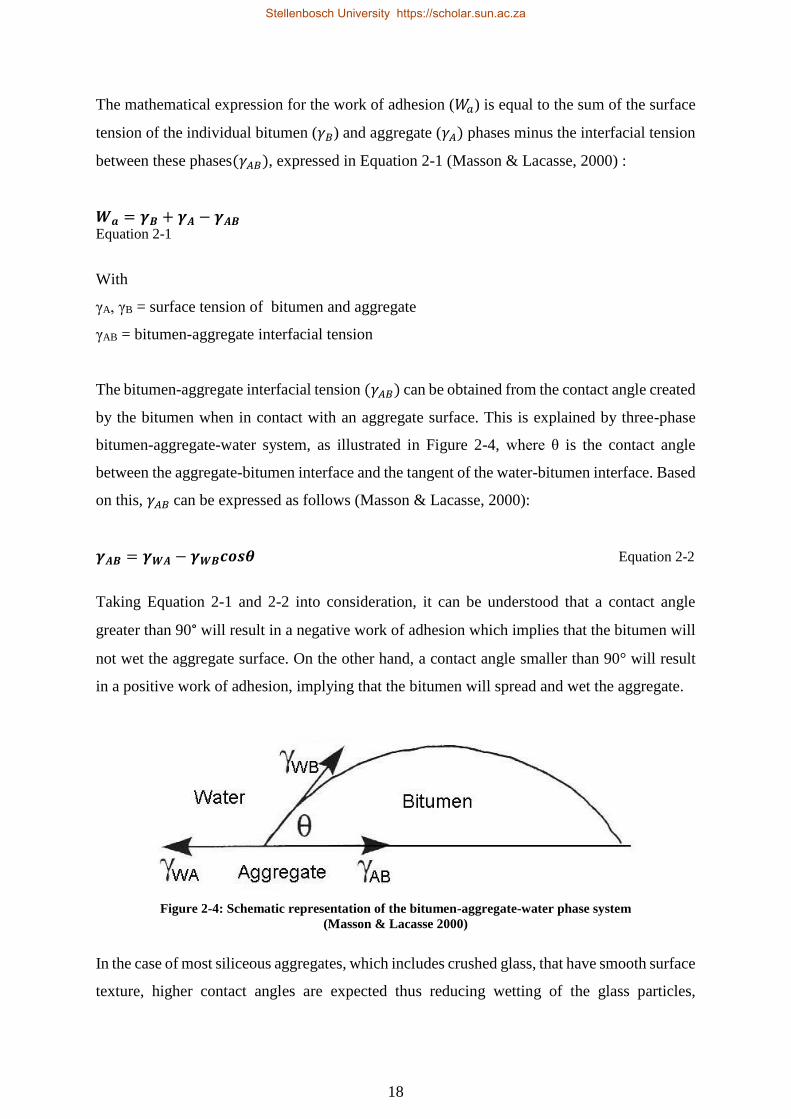
The bitumen-aggregate interfacial tension (𝛾𝐴𝐵) can be obtained from the contact angle created
by the bitumen when in contact with an aggregate surface. This is explained by three-phase
bitumen-aggregate-water system, as illustrated in Figure 2-4, where θ is the contact angle
between the aggregate-bitumen interface and the tangent of the water-bitumen interface. Based
on this, 𝛾𝐴𝐵 can be expressed as follows (Masson & Lacasse, 2000):
𝜸𝑨𝑩 = 𝜸𝑾𝑨 − 𝜸𝑾𝑩𝒄𝒐𝒔𝜽 Equation 2-2
Taking Equation 2-1 and 2-2 into consideration, it can be understood that a contact angle
greater than 90° will result in a negative work of adhesion which implies that the bitumen will
not wet the aggregate surface. On the other hand, a contact angle smaller than 90° will result
in a positive work of adhesion, implying that the bitumen will spread and wet the aggregate.
Figure 2-4: Schematic representation of the bitumen-aggregate-water phase system
(Masson & Lacasse 2000)
In the case of most siliceous aggregates, which includes crushed glass, that have smooth surface
texture, higher contact angles are expected thus reducing wetting of the glass particles,
Stellenbosch University https://scholar.sun.ac.za
Page 35
19
resulting in less adhesion. This concept however addresses adhesion in terms of mere physical
contact between the glass aggregate and the bitumen.
Specific Gravity and Relative Density
A study conducted by Dames and Moore (1993) indicated that the specific gravity of coarse
crushed glass (i.e. > 5mm) ranges from 1.96 to 2.41 and 2.49 to 2.52 for fine crushed glass (i.e.
< 5mm). It should be noted that the level of variance in the above values is influenced by the
degree of purity of the crushed glass sample. The specific gravity of crushed glass is much less
than that of crushed natural aggregates which range from 2.60 to 2.83 (Nebraska State
Recycling Association, 1997).
Grading
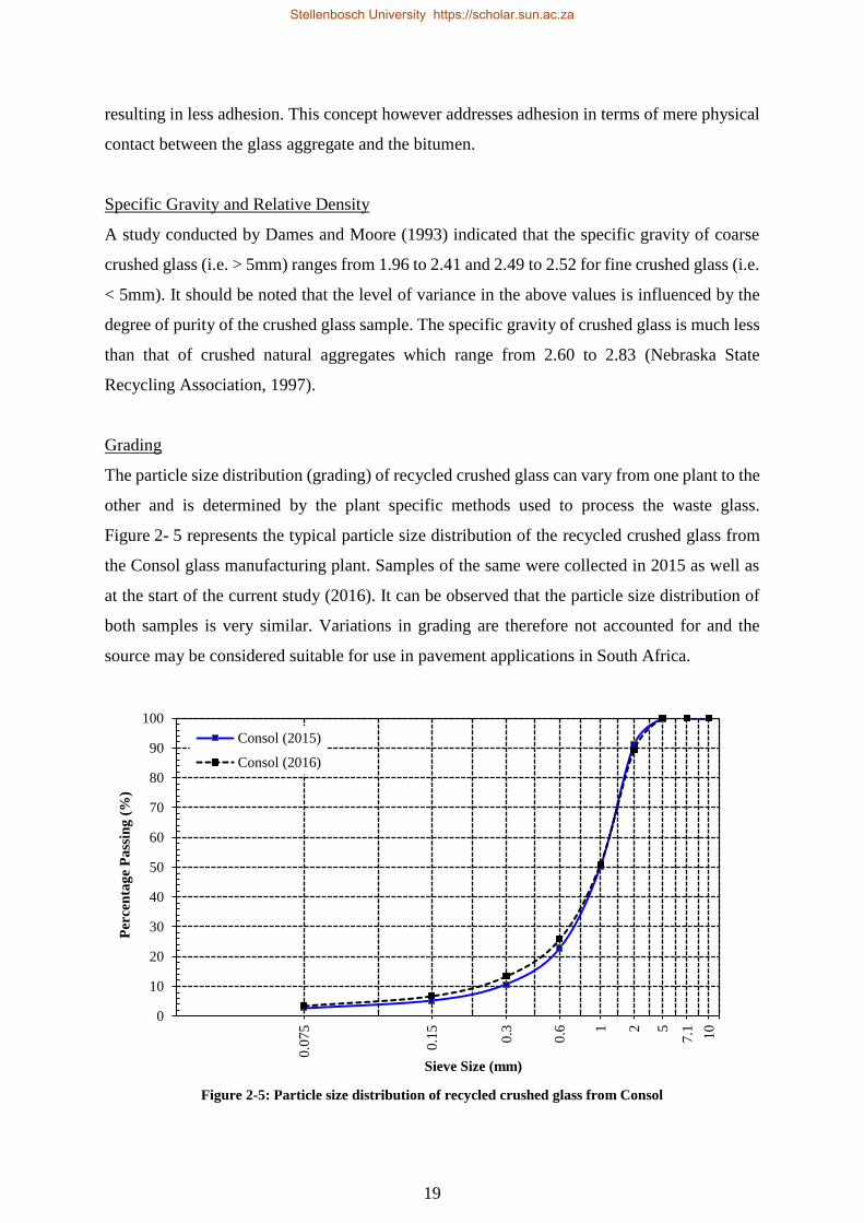
The particle size distribution (grading) of recycled crushed glass can vary from one plant to the
other and is determined by the plant specific methods used to process the waste glass.
Figure 2- 5 represents the typical particle size distribution of the recycled crushed glass from
the Consol glass manufacturing plant. Samples of the same were collected in 2015 as well as
at the start of the current study (2016). It can be observed that the particle size distribution of
both samples is very similar. Variations in grading are therefore not accounted for and the
source may be considered suitable for use in pavement applications in South Africa.
Figure 2-5: Particle size distribution of recycled crushed glass from Consol
0
10
20
30
40
50
60
70
80
90
100
0.0
75
0.1
5
0.3
0.6 1 2 5
7.1 10
Per
cen
tag
e P
ass
ing
(%
)
Sieve Size (mm)
Consol (2015)
Consol (2016)
Stellenbosch University https://scholar.sun.ac.za
Page 36
20
Permeability
The permeability of recycled crushed glass varies with grading (which is known to be
dependent on the level of crushing) as well as quantities utilised, and increases with an increase
in the recycled crushed glass content, particle size and level of contamination (Nebraska State
Recycling Association, 1997). The coefficient of permeability of coarse recycled crushed glass
typically ranges from 10-1 to 10-2 cm/sec which is comparable to the coefficient of permeability
of coarse sand (Federal Highway Administration, n.d.).
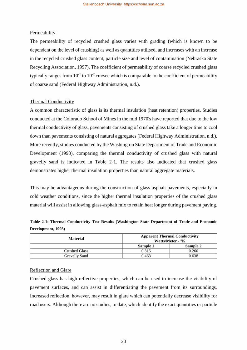
Thermal Conductivity
A common characteristic of glass is its thermal insulation (heat retention) properties. Studies
conducted at the Colorado School of Mines in the mid 1970's have reported that due to the low
thermal conductivity of glass, pavements consisting of crushed glass take a longer time to cool
down than pavements consisting of natural aggregates (Federal Highway Administration, n.d.).
More recently, studies conducted by the Washington State Department of Trade and Economic
Development (1993), comparing the thermal conductivity of crushed glass with natural
gravelly sand is indicated in Table 2-1. The results also indicated that crushed glass
demonstrates higher thermal insulation properties than natural aggregate materials.
This may be advantageous during the construction of glass-asphalt pavements, especially in
cold weather conditions, since the higher thermal insulation properties of the crushed glass
material will assist in allowing glass-asphalt mix to retain heat longer during pavement paving.
Table 2-1: Thermal Conductivity Test Results (Washington State Department of Trade and Economic
Development, 1993)
Material Apparent Thermal Conductivity
Watts/Meter - °K
Sample 1 Sample 2
Crushed Glass 0.315 0.260
Gravelly Sand 0.463 0.638
Reflection and Glare
Crushed glass has high reflective properties, which can be used to increase the visibility of
pavement surfaces, and can assist in differentiating the pavement from its surroundings.
Increased reflection, however, may result in glare which can potentially decrease visibility for
road users. Although there are no studies, to date, which identify the exact quantities or particle
Stellenbosch University https://scholar.sun.ac.za
Page 37
21
size of crushed glass that lead to glare, increased reflection has been has been noticed in
pavements consisting of crushed greater than 15% (Federal Highway Administration, n.d.).
Leachability
Although glass is an inert material, domestic waste glass collection methods could introduce
the presence of contaminants which may affect its chemical characteristics. Typical
contaminants such as lead foil wrappers, for example, may increase the levels of lead in
recycled crushed glass samples. However, waste glass collection and processing methods,
which include removal of contaminants and cleaning, influences the degree of lead
concentration. Large concentrations of contaminants that may however be contained in
recycled crushed glass samples will most likely have an adverse effect on the environment due
to leaching of heavy metals, such as lead, into the soil.
2.1.5.2 Chemical Properties
Mineralogical Composition
Majority of glass bottles and window glass are manufactured from soda-lime glass, which
constitutes a significant portion of the glass produced in South Africa. Table 2-2 lists the typical
chemical composition of this type of glass. For comparative purposes, the chemical
composition of the recycled crushed glass used in this dissertation is also indicated. The
chemical composition was obtained by means of X-ray fluorescence (XRF) analysis on a
sample of the recycled crushed glass. The analysis was conducted at the Council for
Geoscience in Pretoria.
Table 2-2: Typical chemical composition of soda-lime glass (Federal Highway Administration, n.d.)
Constituent Soda-Lime Recycled Crushed Glass
Investigated
SiO2 70 - 73 71.72
Al2O3 1 1.7 - 2.0 2.48
Fe2O3 0.06 - 0.24 0.65
Cr2O3 2 0.1 0.11
Cao 9.1-9.8 10.02
MgO 1.1 - 1.7 0.47
BaO 0.14 - 0.18 0.03
Na2O 13.8 - 14.4 12.85
K2O 0.55 - 0.68 0.50
PbO -- 0.03
B2O3 -- --
1. Higher levels of amber-coloured glass
2. Only present in green glass
Stellenbosch University https://scholar.sun.ac.za
Page 38
22
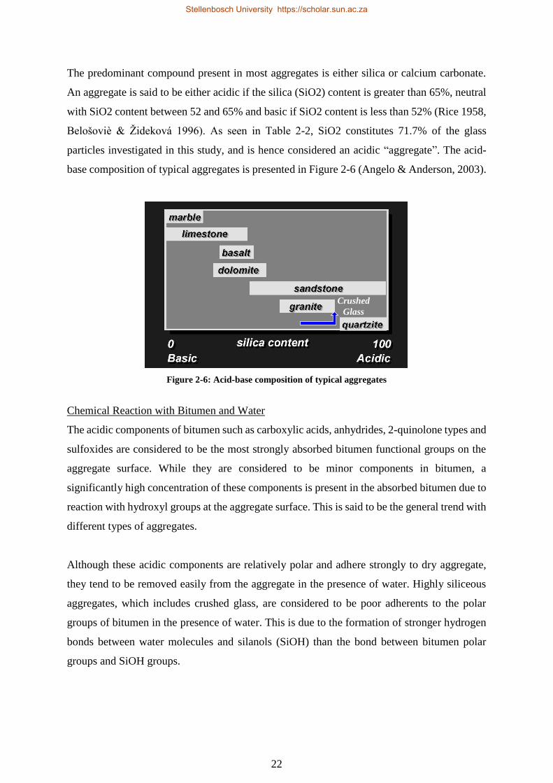
The predominant compound present in most aggregates is either silica or calcium carbonate.
An aggregate is said to be either acidic if the silica (SiO2) content is greater than 65%, neutral
with SiO2 content between 52 and 65% and basic if SiO2 content is less than 52% (Rice 1958,
Belošoviè & Žideková 1996). As seen in Table 2-2, SiO2 constitutes 71.7% of the glass
particles investigated in this study, and is hence considered an acidic “aggregate”. The acid-
base composition of typical aggregates is presented in Figure 2-6 (Angelo & Anderson, 2003).
Figure 2-6: Acid-base composition of typical aggregates
Chemical Reaction with Bitumen and Water
The acidic components of bitumen such as carboxylic acids, anhydrides, 2-quinolone types and
sulfoxides are considered to be the most strongly absorbed bitumen functional groups on the
aggregate surface. While they are considered to be minor components in bitumen, a
significantly high concentration of these components is present in the absorbed bitumen due to
reaction with hydroxyl groups at the aggregate surface. This is said to be the general trend with
different types of aggregates.
Although these acidic components are relatively polar and adhere strongly to dry aggregate,
they tend to be removed easily from the aggregate in the presence of water. Highly siliceous
aggregates, which includes crushed glass, are considered to be poor adherents to the polar
groups of bitumen in the presence of water. This is due to the formation of stronger hydrogen
bonds between water molecules and silanols (SiOH) than the bond between bitumen polar
groups and SiOH groups.
Crushed
Glass
Stellenbosch University https://scholar.sun.ac.za
Page 39
23
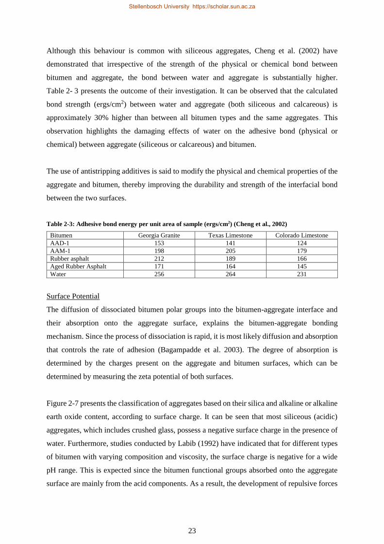
Although this behaviour is common with siliceous aggregates, Cheng et al. (2002) have
demonstrated that irrespective of the strength of the physical or chemical bond between
bitumen and aggregate, the bond between water and aggregate is substantially higher.
Table 2- 3 presents the outcome of their investigation. It can be observed that the calculated
bond strength (ergs/cm2) between water and aggregate (both siliceous and calcareous) is
approximately 30% higher than between all bitumen types and the same aggregates. This
observation highlights the damaging effects of water on the adhesive bond (physical or
chemical) between aggregate (siliceous or calcareous) and bitumen.
The use of antistripping additives is said to modify the physical and chemical properties of the
aggregate and bitumen, thereby improving the durability and strength of the interfacial bond
between the two surfaces.
Table 2-3: Adhesive bond energy per unit area of sample (ergs/cm2) (Cheng et al., 2002)
Bitumen Georgia Granite Texas Limestone Colorado Limestone
AAD-1 153 141 124
AAM-1 198 205 179
Rubber asphalt 212 189 166
Aged Rubber Asphalt 171 164 145
Water 256 264 231
Surface Potential
The diffusion of dissociated bitumen polar groups into the bitumen-aggregate interface and
their absorption onto the aggregate surface, explains the bitumen-aggregate bonding
mechanism. Since the process of dissociation is rapid, it is most likely diffusion and absorption
that controls the rate of adhesion (Bagampadde et al. 2003). The degree of absorption is
determined by the charges present on the aggregate and bitumen surfaces, which can be
determined by measuring the zeta potential of both surfaces.
Figure 2-7 presents the classification of aggregates based on their silica and alkaline or alkaline
earth oxide content, according to surface charge. It can be seen that most siliceous (acidic)
aggregates, which includes crushed glass, possess a negative surface charge in the presence of
water. Furthermore, studies conducted by Labib (1992) have indicated that for different types
of bitumen with varying composition and viscosity, the surface charge is negative for a wide
pH range. This is expected since the bitumen functional groups absorbed onto the aggregate
surface are mainly from the acid components. As a result, the development of repulsive forces
Stellenbosch University https://scholar.sun.ac.za
Page 40
24
between the negatively charged siliceous glass aggregate and bitumen surfaces can occur which
can contribute towards the detachment of bitumen from the glass aggregate surface.
Figure 2-7: Classification of aggregates based on surface charge (Mertens & Wright, 1959)
2.2 Crushed Glass in Hot-Mix-Asphalt
Crushed glass may be used within a specified percentage, as a fine aggregate substitute, in Hot
Mix Asphalt (HMA) pavements. The term "glasphalt or glass-asphalt" has at times been used
to describe these pavements. Even though HMA pavements which have incorporated crushed
glass have shown good performance, the following areas of concern have been identified
(Federal Highway Administration, 1998):
1) Reduced adhesion at the bitumen and glass interface.
2) Potential loss of skid resistance
3) Breakage of larger sized glass particles
4) Increased susceptibility to stripping and ravelling
To avoid the above mentioned concerns, quantities of crushed glass should be limited to 15%
in the surface course of HMA pavements (Federal Highway Administration, 1998). HMA
pavements incorporating quantities in excess of 15% in the surface course may potentially
experience stripping of the bitumen from the glass particles, which can ultimately lead to
deterioration of the pavement. There is, however, the possibility of including larger quantities
of up to 25% when using crushed glass as part of the base or binder course (layer between
surface and base course) in HMA pavements.
In addition, the particle size of crushed glass is an important factor to take into consideration.
Various research studies have established that using small crushed glass with a maximum
Stellenbosch University https://scholar.sun.ac.za
Page 41
25
particle size of 10 mm can address the potential problems mentioned above, while other studies
have indicated that crushed glass should be smaller than 5 mm to have a marked effect on
improved asphalt performance (Hughes, 1990; VTRC, 1998; Wu et al., 2003).
The incorporation of crushed glass in HMA also provides an added advantage over traditional
aggregates due to the low absorption properties of glass. This may allow asphalt mixes to utilise
less bitumen without possibly having an impact on field performance. Although this may be
beneficial from an economic and environmental perspective, the low absorptive properties may
contribute towards stripping of the binder from the glass particles. However, to counter this
effect the use of anti-stripping additives has been recommended for inclusion in glass-asphalt
mixes. Hydrated lime and amine based liquid antistripping additives are most commonly used.
The chemical interaction of these antistripping additives with siliceous glass “aggregates” are
explained below.
Hydrated Lime
As previously mentioned, the hydrogen bonds formed between carboxylic acids in bitumen
and silanols of siliceous glass particles are easily removed in the presence of water, thereby
contributing to poor adhesion between the bitumen and glass aggregate surface. Through the
addition of hydrated lime (Ca(OH)2), the absorption of these water-sensitive carboxylic acids
can be prevented by converting them into insoluble salts. Insoluble calcium organic salts are
formed when the Ca2+ ions from the lime react with the carboxylic acids and 2-quinolenes from
the bitumen. The formation of these strong bonds contribute to improved adhesion (Petersen,
2002).
Schmidt and Graf (1972) have indicated that improved adhesion achieved by hydrated lime is
not entirely due to the reaction between the Ca2+ ions from the lime and the carboxylic acids
and 2-quinolenes from the bitumen but can also be due to the migration of Ca2+ ions to the
surface of the aggregate, where hydrogen, sodium, potassium, or other cations are replaced.
This results in calcium rich bonding sites for bitumen acidic groups.
Additionally, studies conducted by Robert et al. (1996) have revealed that hydrated lime forms
strong bonds with most siliceous aggregates through the formation of a calcium silicate crust
on the surface of the aggregate which has adequate porosity for binder penetration.
Stellenbosch University https://scholar.sun.ac.za
Page 42
26
Liquid Antistripping Additive
Amine based liquid anti-stripping additives are known to improve the adhesion of bitumen
with siliceous aggregates. This is attributed to hydrogen bonding between the polar amine end
group and the silanols of the siliceous aggregate and anchoring of the hydrocarbon chain of the
amine in the bitumen. The long hydrocarbon chain of the amines forms a bridge between the
siliceous aggregate and the bitumen surface, resulting in a strong adhesive bond between the
two surfaces (Tarrer & Wagh, 1991). Two typical amine groups, i.e. primary and tertiary, are
schematically presented in Figure 2-8.
Figure 2-8: Schematic representation of typical amine groups
Numerous studies on the utilisation of crushed glass in HMA and the effect on the volumetric
and mechanical performance properties as well as insitu performance (in some studies) have
been conducted by various researchers and are described in detail below.
Hughes (1990) investigated the technical feasibility of utilising crushed glass as a substitute
aggregate in HMA. The crushed glass utilised in the study was obtained from a contractor in
New York who at the time had constructed a significant number of glass asphalt pavements.
The maximum particle size (MPS) of the glass utilised was 10 mm. The particle size
distribution of the glass material is indicated in Figure 2-9 and represents a similar grading to
that of coarse sand. It should be noted that for comparative purposes, the particle size
distribution of the glass material used in this dissertation is also shown. Comparatively, a much
finer grading can be observed with 100% passing the 5 mm sieve as opposed to 70% passing
the 5 mm sieve in Hughes’ study.
Primary Amine
Tertiary Amine
non-polar hydrocarbon chain polar end group
Stellenbosch University https://scholar.sun.ac.za
Page 43
27
Figure 2-9: Particle size distribution of crushed glass utilised in HMA
The combined grading of the individual aggregates and filler material used to produce an
asphalt mix is referred to as the design grading. The design grading of the glass-asphalt mix
used in Hughes’ study was a 10 mm nominal maximum particle size (NMPS) medium
continuously graded asphalt mix. NMPS is defined in Sabita Manual 35/TRH8 (2016) as “one
sieve size larger than the largest sieve to retain a minimum of 15 percent of the aggregate
particles”.
The investigation entailed a comparison of the volumetric properties of the asphalt mix
consisting of 5% and 15% glass with the volumetric properties of the same asphalt mix without
glass (control mix). It was indicated that the control mix that was selected for the study is
typically used as a wearing course in asphalt pavements in the state of Virginia. The proportion
of glass that was incorporated into the mix substituted a portion of the sand as well as a portion
of the fine and coarse aggregates utilised in the study. The design grading of the glass-asphalt
mixes were similar to the design grading of the control mix. An optimum binder content of
5.75% for the control mix was determined at 5% air voids at a 75-blow compactive effort. The
same optimum binder content was used for the two glass-asphalt mixes (i.e. at 5% and 15%
glass content).
0
10
20
30
40
50
60
70
80
90
100
0.0
75
0.1
5
0.3
0.6 1 2 5
10
14
Per
cen
tag
e P
ass
ing
(%
)
Sieve Size (mm)
Hughes (1990)
Consol (2016)
Stellenbosch University https://scholar.sun.ac.za
Page 44
28
The volumetric properties that were obtained as part of the investigation are indicated in
Figure 2-10. The voids in the mineral aggregate (VMA) and the voids filled with binder (VFB)
in the asphalt mixes were obtained at the determined optimum binder content of 5.75%. The
results revealed that with the addition of 15% crushed glass, a decrease in the voids in the mix
(VIM) and VMA and an increase in the VFB in comparison with the control mix were
observed. It was indicated that the highly angular particle shape and smooth texture of the glass
particles were contributing factors to the observed volumetric properties. Due to the highly
angular particle shape and smooth texture of the crushed glass and the observed effect on the
volumetric properties it was recommended that the optimum binder content for the target
percentage of crushed glass to be incorporated in the mix be determined.
Figure 2-10: Volumetric properties for asphalt mix containing glass at 5.75% binder content
(Hughes, 1990)
The study also included an assessment of the mixes to resist moisture damage. The parameter
used to assess the moisture damage was the tensile strength ratio (TSR) which is a ratio of the
indirect tensile strength of a set of specimens conditioned by moisture to the tensile strength of
a set of unconditioned specimens. TSR values range from 0 (which indicates no resistance to
moisture damage) to 1.0 (which indicates no susceptibility to moisture damage).
One percent (1%) hydrated lime was used in the glass-asphalt mixes as an antistripping additive
to help prevent the loss of adhesion between the bitumen and the glass particles in the presence
of moisture. The control mix, however, did not include an antistripping additive.
The moisture damage test revealed that the addition of 5% of crushed glass had a minor effect
on both the conditioned strength and the TSR values in comparison with the control mix. The
TSR of the glass-asphalt mix constituting 15% crushed glass was approximately 0.9. Though
17
18
19
20
21
22
0 5 10 15 20
VM
A (
%)
Glass Content (%)
50
60
70
80
90
0 5 10 15 20
VF
B (
%)
Glass Content (%)
3
4
5
6
7
8
0 5 10 15 20
VIM
(%
)
Glass Content (%)
Stellenbosch University https://scholar.sun.ac.za
Page 45
29
the conditioned strength and the TSR values were not considerably affected by the percentage
composition of crushed glass, some detachment of the binder from the glass particles was
observed. The inclusion of more coarse crushed glass in the mix was believed to contribute
towards this observation.
Based on the study conducted by Hughes (1990), it was recommended that a maximum of 15%
crushed glass may be used in asphalt mixes provided that the crushed glass adheres with
grading controls to be 100% passing the 9.5mm sieve and not more than 6% passing the
0.075mm sieve. Furthermore, it was recommended that moisture damage tests should be
conducted on glass-asphalt mixes in particular and must produce a TSR value of 0.9 or higher.
This is a more severe requirement for resistance to moisture damage than for mixes not using
crushed glass, however, it was suggested to be reasonable due to the propensity of glass to
suffer moisture damage.
The Virginia Transportation Research Council (VTRC) (1998) conducted an extensive
laboratory study to determine the maximum amount of crushed glass that can be used in HMA
without compromising on the stripping resistance. Stripping in a mix occurs due to the loss of
adhesion between the binder and the aggregate in the presence of moisture. The study was
conducted based on the interest that was expressed by the Virginia Department of
Transportation (VDOT) on the utilisation of crushed glass in asphalt pavements.
Asphalt mixes, each containing hydrated lime and a chemical antistripping additive, were
produced at varying crushed glass contents (0, 5, 12 and 20%). Recycled crushed glass with a
MPS of 10 mm, obtained from a glass recycling plant in Fairfax, Virginia, was used in the
asphalt mixes due to its availability from the same source of glass used in a number of test
sections in Virginia, which also did not require additional crushing.
The TSR parameter was used to evaluate the stripping resistance of the glass-asphalt mixes. A
TSR value of 0.90 was used to determine the maximum crushed glass content that could safely
be used in asphalt mixes. The VDOT usually specifies a minimum TSR value of 0.85; however,
0.90 was specified in order to ensure a higher resistance to stripping in the glass-asphalt mix.
Stellenbosch University https://scholar.sun.ac.za
Page 46
30
The design grading used to manufacture the glass-asphalt mixes was a 14 mm NMPS fine
continuously-graded mix. It was indicated that a constant design grading was maintained for
all the mixes i.e. at 0, 5, 12 and 20% crushed glass content.
It was observed from the results that the mixes with no additives produced TSR values in the
0.7 to 0.8 range. However, with the addition of the antistripping additives the mixes consisting
of both additives produced TSR’s of approximately 0.85 or above. This was, however, only
relevant for the mixes containing up to 12% crushed glass content.
Furthermore, the results revealed that the mixes with hydrated lime indicated the least variance
(approximately 0.05) in TSR values with increasing crushed glass content. This behaviour
indicated that the stripping resistance of the mix may be maintained at a certain level with the
addition of hydrated lime as opposed to the chemical additive which showed a decline in the
TSR results as the glass content increased.
In addition, a comparison of the mixes consisting of 20% crushed glass showed that the mix
containing the chemical additive had a significantly lower average wet (conditioned) strength
than that of the mix with hydrated lime. However, the mixes consisting of lower glass content
did not show any significant variance in average wet strength.
The study, therefore, concluded that up to 15% of crushed glass in asphalt, with hydrated lime
serving as an anti-stripping additive, is acceptable to prevent stripping of glass-asphalt. It
should be noted that the findings of the study was centred on the assumption that the TSR, as
a performance indicator, reliably predicts field stripping. Furthermore it was indicated that the
proposed acceptable crushed glass content may vary with different mix types as well as well
as for different grading of crushed glass.
Based on the above results, the VDOT has recommended that standards in Virginia specifying
a maximum glass content of 15% in HMA be maintained.
Wu et al. (2003) conducted a comprehensive laboratory study to determine the optimal
percentage of crushed glass that can be incorporated into an asphalt mix. The investigation was
conducted on four asphalt mixes consisting of 0, 5, 10, 15 and 20% of crushed glass. The glass
material utilised in the study was obtained by manually crushing reclaimed beer bottles.
Stellenbosch University https://scholar.sun.ac.za
Page 47
31
The investigation included a preliminary study to determine the MPS of crushed glass that can
be incorporated into the asphalt mixes which would ensure maximum adhesion between the
glass particles and the bitumen in the presence of moisture. The Hamburg Wheel Tracking Test
(HWTT) was used to assess the moisture susceptibility of the asphalt mixes with a maximum
glass particle size of 10 mm in comparison with a maximum glass particle size of 5 mm. The
HWTT measures the collective effect of rutting and moisture damage by means of a rubber
wheel that traverses in both directions across an asphalt specimen which is submerged in a
water bath at a specified test temperature.
It was observed after the HWTT that there were much more uncovered surface areas in the
mixes with a maximum glass particle size of 10 mm (Mix A) as opposed to the mixes with a
maximum glass particle size of 5 mm (Mix B) - see Figure 2-11. This may be due to the larger
number of fractured faces of the fine crushed glass particles as opposed to the coarse glass
particles, which in turn increases the physical area of contact and hence improves adhesion at
the bitumen aggregate interface. The larger number of fractured faces may also prevent an
abrupt plane of stress transfer, where the stresses are rather transferred across or into the
bitumen, resulting in less stripping.
Furthermore, the HWTT results revealed that the dynamic stability of the Mix A was
considerably lower than Mix B. The dynamic stability is measured as the number of passes per
mm rut depth obtained from the HWTT. Based on the above observations, the preliminary
study therefore concluded that the utilisation of crushed glass with a MPS of 10 mm was not
viable. A maximum glass particle size of 5 mm was hence adopted for the primary
investigation.
Figure 2-11: 10 mm (left) and 5 mm (right) maximum glass particle size in asphalt mix (Wu et al., 2003)
Stellenbosch University https://scholar.sun.ac.za
Page 48
32
The particle size distribution of the manually crushed reclaimed beer bottles that was used in
the primary investigation is indicated in in Figure 2-12. It should be noted that for comparative
purposes, the particle size distribution of the glass material used in this dissertation is also
indicated. It can be observed that the grading of the crushed glass material is relatively similar
except between a particle size of 1mm and 5 mm, where the glass used in Wu et al.’s study is
20% coarser.
Figure 2-12: Particle size distribution of crushed glass used in HMA
Similar to the preliminary study, the HWTT was conducted on the asphalt mixes constituting
0, 5, 10, 15 and 20% of crushed glass. The determining parameters that were investigated to
select the optimal mix were based on the permanent rutting deformation and stripping weight
loss of the asphalt mixes obtained from the HWTT. The stripping weight loss is measured by
comparing the weight of the mixes before testing (unconditioned samples) in comparison with
the weight of the mixes after the HWTT. It should be noted that the test temperature was
selected at 45°C due to the samples dispersing at the specified high temperature of 60°C.
The design grading used to manufacture the glass-asphalt mixes was a 14 mm NMPS medium
continuously-graded glass-asphalt mix. It was indicated that the design grading was similar for
all the crushed glass contents. The optimum binder content of the mix with no glass (control
mix) was determined to be 4.8% at 4.13% air voids. Similar to Hughes’s (1990) study; the
0
10
20
30
40
50
60
70
80
90
100
0.0
75
0.1
5
0.3
0.6 1 2 5
10
Per
cen
tag
e P
ass
ing
(%
)
Sieve Size (mm)
Wu et al. (2003)
Consol (2016)
Stellenbosch University https://scholar.sun.ac.za
Page 49
33
same binder content was used for the different glass-asphalt mixes (i.e. at 5%, 10%, 15% and
20% crushed glass content).
The HWTT revealed an increase in permanent rutting deformation and stripping weight loss
with increasing crushed glass content, as indicated in Table 2-4.
Table 2-4: Hamburg wheel tracking test results (Wu et al., 2003)
Glass Replacement
(%)
Rutting Deformation
(mm)
Stripping Weight
(g) Remarks
0 9.80 15.60
*sample was broken at a
rut depth of 13.7mm
5 10.6 23.40
10 13.6 49.50
15 15.0 88.70
20 13.7 230.3
Furthermore, it was observed that the asphalt samples with higher crushed glass content (i.e. at
15%) had reached a maximum rut depth of 15 mm after a much shorter period of time. The
obtained rut depth with respect to loading times is illustrated in Figure 2-13. In addition, it was
revealed that the start of asphalt stripping of the glass-asphalt mixes occurred at less than 1500
loading repetitions. The addition of crushed glass, therefore, proved to have a negative effect
on the moisture susceptibility of the asphalt mixes particularly at higher contents (i.e. at 15 and
20%). Based on the above observations, it was identified that a more conservative optimum
crushed glass content was achieved using a 10% replacement ratio.
Figure 2-13: Rut depth with respect to loading repetitions (Wu et al., 2003)
The study consequently proceeded to investigate the effect of the addition of antistripping
agents namely, hydrated lime and a liquid anti-stripping agent namely, coconut ethanolamine,
Glass Content (%)
Stellenbosch University https://scholar.sun.ac.za
Page 50
34
on the permanent rutting deformation and moisture susceptibility of the selected optimal mix
(i.e. at 10% crushed glass content).
Trial tests conducted on the optimal mix, firstly with 2% hydrated lime and secondly with 0.4%
(by mass of bitumen) of the liquid anti-stripping agent, demonstrated a substantial
improvement in resistance to rutting deformation as well as moisture damage in comparison
with the same mix without an anti-stripping agent. It was also interesting to note that the rutting
deformation results were comparable to the mix without glass. Furthermore, the results
indicated that the liquid anti-stripping agent was more effective than the hydrated lime in
resisting rutting deformation and moisture damage.
Figure 2-14 shows the internal state of the broken glass-asphalt sample (i.e. at 10% crushed
glass content) tested before and after the addition of the liquid anti-stripping agent. It can be
seen that some aggregate surfaces are not coated with bitumen in the sample without the anti-
stripping agent (left) as opposed to the sample with the anti-stripping agent where no exposed
aggregate surfaces are displayed (right).
Figure 2-14: Glass asphalt mix prior to (left) and post (right) use of liquid anti-stripping agent
(Wu et al., 2003)
Based on the study conducted by Wu et al. (2003) it was recommended that large glass particles
(i.e. larger than 5 mm) should be avoided when utilised as an aggregate replacement in asphalt
mixes. The following areas of concern were addressed:
An increase in the size of the aggregate particles results in a smaller surface area causing
weaker adhesive bonds between the glass particles and the bitumen.
Stellenbosch University https://scholar.sun.ac.za
Page 51
35
The smooth surface texture of large glass particles contributes to the formation of weak
adhesive bonds between the glass particles and the bitumen.
Large glass particles may cause significant abrasion of car tyres as well as reduction in skid
resistance caused due to the breakage of the large glass particles by traffic loading.
It was hence recommended that smaller glass particles (less than 5 mm) should be utilised in
asphalt mixes since the presence of more fragmentised and textured surfaces of smaller
particles aid in promoting adhesion between bitumen and glass particles.
Su & Chen (2002) conducted a study to determine the feasibility of utilising recovered
domestic waste glass with the aim of using it as an aggregate substitute in HMA. The
investigation entailed a comprehensive laboratory study whereby four glass contents i.e. 0, 5,
10 and 15% by weight of total aggregate were utilised as a partial aggregate replacement to
develop four asphalt mixes.
The glass that was utilised was manually crushed and thereafter pulverised to a MPS of 5 mm.
The particle size distribution of the crushed glass is indicated in Figure 2-15. For comparative
purposes, the particle size distribution of the glass material used in this dissertation is also
indicated. A different approach was adopted in replacing the aggregate with the crushed glass.
The approach involved substituting each percentage composition of crushed glass of a specific
particle size with the same content and particle size of the virgin aggregate.
Stellenbosch University https://scholar.sun.ac.za
Page 52
36
Figure 2-15: Particle size distribution of crushed glass used in HMA
In addition to the above, lime at varying contents (0-3%) were added to each mix to assess the
effect of the varying contents of lime on the stability of the mixes. Stability is a measure of the
resistance of an asphalt mix to permanent deformation and is measured by the maximum load
supported by a test specimen when loaded diametrically at 50.8 mm/minute at 60°C (Pavement
Interactive, n.d.). The obtained stability values at the varying lime contents are illustrated in
Figure 2-16. The addition of 2% lime was observed as the optimum amount of lime to be
included in order to achieve maximum stability of the mix.
Figure 2-16: Stability values of glass asphalt mixes with lime (Su & Chen, 2002)
0
10
20
30
40
50
60
70
80
90
100
0.0
75
0.1
5
0.3
0.6 1 2 5
10
Per
cen
tag
e P
ass
ing
(%
)
Sieve Size (mm)
Su &Chen (2002)
Consol (2016)
6
7
8
9
10
11
12
13
0 1 2 3
Sta
bil
ity
(k
N)
Lime Content (%)
0
5
10
15
Stellenbosch University https://scholar.sun.ac.za
Page 53
37
The design grading used to manufacture the glass-asphalt mixes was a 20 mm NMPS fine
continuously-graded glass-asphalt mix. It was indicated that the design grading was similar for
the four glass-asphalt mixes. As opposed to the investigations carried out by Hughes (1990)
and Wu et al. (2003), the optimum binder content for each percentage composition of glass
was determined, as depicted in Figure 2-17.
Figure 2-17: Optimum binder content of glass-asphalt mixes (Su & Chen, 2002)
The tests that were conducted on the asphalt mixes included both laboratory and field tests, of
which the latter was conducted on three different test sites, funded by the Highway Engineering
Department in Taiwan. The test pavements were constructed with the investigated amounts of
glass (i.e. 0, 5, 10 and 15%) at the respective optimum binder content’s (i.e. 5.32, 5.20, 5.05
and 5.00 %). The reported outcome of both the laboratory and field tests is provided below.
Laboratory test observations:
The optimum binder content varied with respect to the glass content incorporated within
the mix. Furthermore, the optimum binder content decreased as the glass content within the
mixes increased. This phenomenon was attributed to the smooth surface texture of the glass
particles, resulting in a lower rate of binder absorption.
Due to the lower binder absorption rate, it was observed that the film of binder that coated
the glass particles was relatively thin which resulted in weak bonds between the binder and
the glass particles, resulting in durability issues.
The above durability concern was improved with the addition of 2% lime.
5.32
5.20
5.055.00
4.80
4.90
5.00
5.10
5.20
5.30
5.40
0 5 10 15
Op
tim
um
Bin
der
Co
nte
nt
(%)
Glass Replacement (%)
Stellenbosch University https://scholar.sun.ac.za
Page 54
38
Field test observations:
The stability values of all the glass-asphalt filed specimens were found to be “profoundly
greater” than the minimum criteria as specified in the Marshal Test procedure, i.e. 6.68 kN.
It was identified that the light reflection intensities when tested at night increased on the
test sections with increased amounts of crushed glass. As expected the light reflection was
significantly higher than that of asphalt pavements without crushed glass, as shown in
Figure 2-18.
The investigation on skid resistance revealed improved resistance along the longitudinal
and transverse profile of the asphalt pavements as the crushed glass content increased.
It was specifically highlighted that the asphalt pavement that constituted 10% of crushed
glass after one year of service indicated no ravelling of the glass particles as well as no
rutting of the glass-asphalt pavement.
Figure 2-18: Light reflection properties of glass particles demonstrated on asphalt test pavement
(Su & Chen, 2002)
Arabani (2010) conducted a study to investigate the effect of varying contents of crushed glass
on the stiffness modulus of asphalt mixes at different temperatures. The stiffness modulus is a
performance-related parameter used to predict the strength of pavements subjected to dynamic
loading. The stiffness moduli of the mixes were determined by the indirect tensile stiffness
modulus (ITSM) test. A repeated load was applied along the vertical diameter of the test
specimen at a frequency of 1Hz with a load duration of 0.1 seconds and a rest period of 0.9
seconds. The resulting recoverable horizontal tensile strain was measured for determination of
the stiffness modulus.
Stellenbosch University https://scholar.sun.ac.za
Page 55
39
Five asphalt mixes were prepared consisting of 0, 5, 10, 15 and 20% crushed glass and the
optimum binder content of the mixes ranged between 5.5% and 6%. In addition, 2% hydrated
lime was used in the mixes as an antistripping agent.
The crushed glass used in the study was collected from a glass production company in Iran.
The MPS of the glass utilised was 5 mm. The particle size distribution of the crushed glass is
indicated in Figure 2-19. It can be observed that the grading of the crushed glass used in this
dissertation is approximately 10 to 30% finer for a particle size between 1 mm and 2 mm.
Figure 2-19: Particle size distribution of crushed glass utilised in HMA
It was specified that the design grading of the glass-asphalt mix was obtained within the limits
indicated in Table 2-5 and was similar for all crushed glass contents (i.e. 0, 5, 10 15 and 20%).
Table 2-5: Design grading of glass-asphalt mix (Arabani, 2010)
Sieve Size (mm) Percentage of Weight Passing (%)
0.075 2-10
0.3 5-21
2 28-58
5 44-74
14 90-100
20 100
0
10
20
30
40
50
60
70
80
90
100
0.0
75
0.1
5
0.3
0.6 1 2 5
10
Per
cen
tag
e P
ass
ing
(%
)
Sieve Size (mm)
Arabani (2010)
Consol (2016)
Stellenbosch University https://scholar.sun.ac.za
Page 56
40
The obtained stiffness moduli of the glass-asphalt mixes for the varying proportions of crushed
glass as well at three different test temperatures (i.e. 5, 25 and 40 °C) are presented in Figure
2-20.
It was observed that the glass-asphalt mixes demonstrated improved stiffness modulus with an
increase in crushed glass content, whereby the maximum stiffness occurred at 15%. However,
at crushed glass content above 15%, the stiffness modulus of the glass-asphalt mix decreased.
It was indicated that above the optimum crushed glass content (i.e. 15%), the stiffness modulus
of the mix decreases due to the addition of a large number of smooth glass particles as well as
higher quantities of glass in the mix that do not absorb the bitumen adequately resulting in a
more fragile structure.
It was also observed that at different temperatures, the stiffness modulus remained relatively
constant. It was, therefore, suggested that the stiffness modulus of glass-asphalt mixes are at
its maximum at 15% crushed glass content at any specific temperature. In addition, the stiffness
modulus of the glass-asphalt mixes indicated lower sensitivity to variations in temperature
when compared to the asphalt mix without glass. When the test temperature was increased from
5°C to 40°C, the stiffness modulus of the asphalt mix without crushed glass reduced by
approximately 70%, while the stiffness modulus of the glass-asphalt mix (i.e. with 15% crushed
glass content) only experienced a reduction of approximately 50%.
It was indicated that the increased stiffness modulus of the glass-asphalt mixes (excluding the
mix with 20% crushed glass) in comparison with the asphalt mix without crushed glass was
attributed to the highly angular glass particles; allowing for better interlock between the
aggregates and the glass particles.
Stellenbosch University https://scholar.sun.ac.za
Page 57
41
Figure 2-20: Variations of stiffness modulus with temperature at different crushed glass content
(Arabani, 2010)
Lachance-Tremblay et al. (2014) conducted a study to assess and compare the performance
of asphalt mixes consisting of five different contents of crushed glass (5, 10, 15, 20, and 25%)
with an asphalt mix (control mix) without crushed glass. The control mix selected for the study
is standardised by the Quebec Ministry of transportation (MTQ) and is commonly used in
surfacing courses in Quebec. The following performance characteristics of the asphalt mixes
were studied: 1) resistance to rutting, 2) low temperature cracking resistance and 3) stripping
susceptibility.
In this experimental investigation, similar to the study conducted by Su & Chen (2002), two
different sizes of crushed glass i.e. 0 to 0.315 mm and 0.63 to 2.5 mm were used as a substitute
to the natural aggregates used (See Figure 2-21).
0
200
400
600
800
1000
1200
1400
5 25 40
Sti
ffn
ess
Mo
du
lus
(MP
a)
Temperature °C
0%
5%
10%
15%
20%
Stellenbosch University https://scholar.sun.ac.za
Page 58
42
a) 0 to 0.315 mm b) 0.63 to 2.5 mm
Figure 2-21: Different sizes of crushed glass used (Lachance-Tremblay et al., 2014)
The design grading used to manufacture the glass-asphalt mixes was a 14 mm NMPS medium
continuously-graded glass-asphalt mix. It was indicated that the design grading was similar for
all contents of crushed glass (i.e. 5, 10, 15, 20, and 25%) and was designed to represent a
similar design grading to that of the control mix.
The asphalt mix with 10% crushed glass was selected as the optimal mix on which the
performance testing was carried out. This mix was selected based on the voids content being
very similar to the reference mix at 100 gyrations. The optimum binder content of the mix was
determined to be 4.53% at 5.5% air voids.
The rutting resistance of the selected glass and reference asphalt mix was evaluated with the
“French Wheel Tracking Rutting test” using the “MLPC French rutting tester”. The rut depth
of the glass-asphalt mix after 30,000 cycles was approximately 1% lower than the control mix
but was still below the maximum allowable rutting depth (i.e. 10% rut depth at 30 000 cycles).
The cracking resistance of the glass and reference asphalt mix at low temperatures was assessed
by conducting the “thermal stress restrained specimen test (TSRST)”. It was observed that the
average failure stress and failure temperature of both asphalt mixes were the same.
Additionally, it was observed that in both cases the average failure temperature was very close
to the low temperature performance grade of the binder used in the investigation, i.e. -34°C.
The addition of 10% crushed glass, therefore, did not have an effect on the low temperature
performance of the asphalt mix.
Stellenbosch University https://scholar.sun.ac.za
Page 59
43
The “stripping susceptibility test” was used to measure the resistance of the two mixes to
moisture damage. The glass-asphalt mix demonstrated slightly inferior resisting to moisture
damage than the reference mix. It should be mentioned, however, that no anti-stripping agent
was added to the glass-asphalt mixes.
Details on the testing procedure and test specifications of the French Wheel Tracking Rutting
test, TSRST and the stripping susceptibility test are not provided but can be referred to in the
LC 26-410 (equivalent, EN 12697-22), AASHTO TP10-93 and LC 26-001 (equivalent, ASTM
D1075) standards respectively.
Based on the study conducted by Lachance-Tremblay et al. (2014) it was concluded that the
addition of 10% crushed glass can be utilised in asphalt mixes without compromising the
overall performance of the asphalt mix. It was, however, recommended that special attention
must be taken to consider the size of the crushed glass particles as well as to note that a decrease
in resistance to rutting as well as moisture damage may occur due to the lack of adhesion
between the bitumen and the surface of the crushed glass particles. As in previous studies
conducted, it was indicated that this occurrence may be improved with the addition of an anti-
stripping additive.
Anochie-Boateng and George (2016) conducted a study to compare the performance
properties of a continuously-graded asphalt mix containing crushed glass with that of a
traditional asphalt wearing course mix used on South African Roads. The performance of the
asphalt mix was evaluated based on stiffness, permanent deformation and fatigue properties.
The asphalt mix consisted of 15% crushed glass with the addition of 3% hydrated lime
constituting the filler component in the mix, and serving as an antistripping additive to promote
better adhesion between the bitumen and the glass particles. The crushed glass, utilised in the
study, was collected from the same source as the crushed glass utilised in this dissertation. The
particle size distribution of the crushed glass used for both studies is indicated in Section 2.1.5.
The MPS of the glass utilised was 5 mm.
In order to conduct a comparative analysis on the performance of the two mixes, the same
component materials as that of the traditional asphalt mix was utilised in the study. The
traditional mix, however, did not incorporate an antistripping additive but consisted of 1% plant
Stellenbosch University https://scholar.sun.ac.za
Page 60
44
fines (i.e. baghouse fines obtained from the asphalt manufacturing plant) as the filler
component in the mix.
The design grading used to manufacture the glass-asphalt mix was a 10 mm NMPS medium
continuously-graded glass-asphalt mix. The grading was designed to represent a similar design
grading to that of the traditional asphalt mix. The optimum binder content of the glass-asphalt
mix was 5.1% and was determined at 4% air voids. A similar optimum binder content (5.0%)
was obtained for the traditional mix that did not contain crushed glass.
The dynamic modulus test was used to evaluate the stiffness properties of the glass-asphalt mix
in comparison with the traditional mix. It was observed that at a test frequency of 10Hz and a
test temperature of 20°C, the stiffness of the glass-asphalt mix improved by 25%. It was
indicated that the above test conditions best simulate South African field pavement conditions.
The flow number test was used to evaluate the permanent deformation properties of the glass-
asphalt mix and the traditional mix. It is known that asphalt mixes with a higher flow number
demonstrates improved resistance to rutting (permanent deformation) than an asphalt mix with
a lower flow number. The flow number results hence revealed that the glass-asphalt mix has
higher rutting resistance at the tested conditions i.e. temperature of 50°C and stress levels of
276 kPa and 483 kPa than the traditional mix.
The observed behaviour has been attributed, in part, to the increased angularity of the glass
particles which in turn increases the interlock between the glass particles and the aggregate,
thereby contributing towards the improved permanent deformation resistance of the glass-
asphalt mix. In addition, the incorporation of 3% hydrated lime in the glass-asphalt mix was
also indicated to have contributed towards the improved stiffness properties of the glass-asphalt
mix in comparison with the traditional mix, which incorporated 1% plant filler.
The fatigue properties of the two mixes were evaluated using the four-point beam fatigue test.
Fatigue failure in asphalt layers occurs when the number of applied load repetitions surpasses
the ability of the asphalt layer to resist the associated tensile strains. It was observed that the
glass-asphalt mix, at a test frequency of 10Hz and a test temperature of 20°C, showed a
significant reduction in fatigue life at the lower strain levels while comparable fatigue life was
indicated at the higher strain levels.
Stellenbosch University https://scholar.sun.ac.za
Page 61
45
Anochie-Boateng and George (2016) concluded that there is potential to utilise crushed glass
as an aggregate substitute in asphalt wearing course mixes. This conclusion was drawn based
on the improved performance obtained in stiffness and permanent deformation as well as the
comparable fatigue life at high strain levels when compared to the traditional mix investigated
in the study. Furthermore, the observed performance was based on the specified design grading
for the glass-asphalt mix and the traditional mix as well as the component materials utilised to
produce both mixes.
Stellenbosch University https://scholar.sun.ac.za
Page 62
46
2.3 Summary
The literature study highlights the global use of crushed glass in HMA since the early 1970’s.
Countries that have reported using crushed glass in asphalt paving applications include United
States, Canada, United Kingdom, Australia, New Zeland, Japan and Taiwan. Although large
quantities of recycled crushed glass are available for exploitation in South Africa, the local use
of this material in South African pavements has, however, not been utilised thus far and hence
forms the basis for investigation in this study.
The literature study also highlights various favourable properties of crushed glass material for
incorporation as an aggregate substitute in asphalt pavement applications. Such properties
include the highly angular shape characteristics, low specific gravity, high thermal insulation
properties as well as the high reflective properties of crushed glass material.
The smooth surface texture of glass material has, however, been emphasised as a contributory
factor towards reduced adhesion at the bitumen and glass interface resulting in an increased
susceptibility to stripping and ravelling in glass-asphalt pavements in comparison with
traditional asphalt pavements. To avoid these concerns, various studies have limited the use of
crushed glass up to 15% in the surface course with control limits set on the grading of the glass
particles used. Few studies have also reported on the incorporation of various antistripping
additives which have shown a marked improvement on the moisture susceptibility of glass-
asphalt mixes and as such have been known to alleviate the common stripping related concerns.
In addition, certain studies have indicated improved performance in terms of rutting and
stiffness in HMA pavements incorporating up to 15% crushed glass above which reduced
performance has been reported.
It was, however, noted that the studies reported have drawn conclusions and proposed
recommendations on the use of crushed glass in asphalt mixes that are typical to a specific
country or state while utilising the crushed glass material in combination with different types
of coarse and fine aggregates common to a particular region. In addition the crushed glass
material has in some cases been manually engineered to obtain a specific particle size
distribution while in other cases the material has been used as obtained from their local glass
manufacturing plants or material recovery facilities, which varies from one study to the other.
Such variations including variations that arise from the use of different types of raw materials
e.g. binder, filler material, antistripping additives etc. as well as different testing methodologies
Stellenbosch University https://scholar.sun.ac.za
Page 63
47
and specifications (applicable to a specific country or state) may have an influence on the
observed performance reported in the various investigations detailed in the literature study.
Stellenbosch University https://scholar.sun.ac.za
Page 64
48
3. GLASS-ASPHALT MIX DESIGN
3.1. Introduction
Chapter 3 presents the design and production of a 10 mm nominal maximum particle size,
medium continuously-graded glass-asphalt mix that consists of 15% recycled crushed glass as
a partial substitute to the traditional fine aggregate in the mix. This percentage composition of
recycled crushed glass was selected based on the findings from various studies (highlighted in
Chapter 2) indicating an optimum crushed glass replacement ratio of 10 to 15%.
Three of the above glass-asphalt mixes were produced; with the first mix (referred to as GA
Mix1) containing 1% hydrated lime which constitutes the filler component and acts as an
antistripping additive. The second mix (referred to as GA Mix 2) consists of 1% “plant filler”
(baghouse fines from asphalt manufacturing plant) as the filler component and contains a liquid
antistripping additive. The third mix (referred to as GA Mix 3) comprises of the same filler
component as GA Mix 2 (1% plant filler) and does not contain an antistripping additive. All
three glass-asphalt mixes utilises the same aggregate materials. The incorporation of 1%
hydrated lime was selected based on the maximum specified amount allowed for inclusion in
continuously-graded asphalt mixes in South Africa (Sabita, 2016).
The glass-asphalt mixes are designed as a surfacing course with a design traffic level between
3 and 30 million Equivalent Standard Axle Loads (ESALs) and represents a similar design
aggregate grading to the South African National Roads Agency Limited (SANRAL) medium
continuously-graded asphalt mix (herein after referred to as the standard mix). It has been indicated
that the standard asphalt mix is commonly used as a surfacing course on South African roads.
Furthermore, to maintain consistency, the same aggregates as well as the same binder i.e. 50-70
penetration grade binder, utilised in the standard mix, was used to prepare the glass-asphalt mixes.
The glass-asphalt mix design and production makes use of standard design practices for
traditional asphalt mixes in South Africa and is conducted in accordance with Sabita Manual
35/TRH 8 (2016) – “Design and Use of Asphalt in Road Pavements”.
Stellenbosch University https://scholar.sun.ac.za
Page 65
49
3.2. Raw Materials
3.2.1. Aggregate
The same aggregates from the same sources as the standard mix were utilised in this study. The
aggregate materials and sources are provided in Table 3-1. The aggregate sources are all located
in the Gauteng province.
Table 3-1: Aggregate Material and Sources
Aggregate Fractions Aggregate Source
Andesite 9.5 mm
AfriSam Eikenhof Andesite 6.7 mm
Andesite Crusher dust (CD)
Granite Crusher sand (CS) AfriSam Jukskei
Mine sand Benoni Summit
As indicated in Chapter 2, the recycled crushed glass was sourced from the Consol
manufacturing plant located in Gauteng. Physical characterisation of the recycled crushed glass
particles is discussed in detail in Section 3.7.
The aggregates and glass material were dried in an oven at a temperature of 105°C for a
duration of 16 hours, after which the materials were split down by riffling to the approximate
quantities required by the mix. Wet sieve analysis was conducted on the individual aggregate
fractions as well as on the glass material. Photographs of the glass material retained on each
standard sieve is presented in Figure 3-1. The sieve analysis was conducted in accordance with
South African National Standard (SANS) 3001-AG1 (2014). The results are presented in Table
3-3 and illustrated graphically in Figure 3-2.
Stellenbosch University https://scholar.sun.ac.za
Page 66
50
4.75 mm
2.36 mm
1.18 mm
0.60 mm
0.30 mm
0.15 mm
0.075 mm
Figure 3-1: Photographs of recycled crushed glass particles retained on standard sieve size
Stellenbosch University https://scholar.sun.ac.za
Page 67
51
Figure 3-2: Particle size distribution of individual aggregate fractions
3.2.2. Filler
Hydrated lime, supplied by Lime Distributors (Pty) Ltd., and baghouse fines (referred to as
plant filler and comprising mainly of SiO2), obtained from the Much Asphalt plant in Eikenhof,
were used as the mineral filler component in GA Mix 1 and GA Mix 2, 3 respectively. The
hydrated lime and plant filler has a particle size range between 1.5 and 75 µm and 0.4 and
75 µm respectively.
3.2.3. Bituminous Binder
A 50-70 penetration grade binder, manufactured by the National Petroleum Refiners of
South Africa (Pty) Ltd. (Natref), was obtained from the Much Asphalt plant in Benoni. The
properties of the binder were determined as per the relevant standard test method indicated in
Table 3-2. Tests were conducted on the original binder as well as on the binder subjected to
the Rolling Thin Film Oven Test (RTFOT – to simulate ageing that occurs during manufacture
and laying of the mix). The tests were conducted at the Advanced Materials Testing Laboratory
at the CSIR.
0
10
20
30
40
50
60
70
80
90
100
0.0
75
0.1
5
0.3
0.6 1 2 5
7.1 10
14
Per
cen
tag
e P
ass
ing
(%
)
Sieve Size (mm)
9.5
Andesite6.7
AndesiteCS
GraniteCD
AndesiteMine
SandWaste
Glass
Stellenbosch University https://scholar.sun.ac.za
Page 68
52
Based on the results presented in Table 3-2, it can be seen that the properties of the binder
comply with the requirements as specified in SANS 4001 BT1 (2016).
Table 3-2: Properties of the 50-70 Penetration Grade Binder
Properties Unit Test Results Requirement Test Method
Penetration dmm 65 50-70 EN 1426
Softening Point °C 47.4 46-56 ASTM D36M
Viscosity
at 60°C Pa.s 256 >120 ASTM D4402M
at 135°C mPa.s 493 220-500 ASTM D4402M
Flash Point °C 328 ≥230 ASTM D92
Spot Test % xylene Negative up to 30 Negative up to 30 AASHTO T102
After RTFOT-ageing
Mass Change %m/m 0.096 0.3 max ASTM D2872
Viscosity at 60°C Pa.s 658 ASTM D4402M
% original % original 257 300 max ASTM D4402M
Softening Point °C 53.4 48 min ASTM D36M
Increase °C 6 7 max ASTM D36M
Penetration dmm 43 EN 1426
% original % original 66 55 min EN 1426
3.2.4. Antistripping Additives
Hydrated lime and a liquid additive, namely WETFIX BE, were applied as antistripping
additives. Much Asphalt among other asphalt manufacturing companies in South Africa has
indicated use of the above mentioned liquid additive as an adhesion promoter in Hot Mix
Asphalt. A dosage amount of 0.5% of WETFIX BE (by volume of binder), as recommended
by the supplier, was added to the binder.
The application process of the liquid additive to the binder involved heating the original binder
to approximately 150°C (mixing temperature), maintaining the same temperature on a hot plate
while blending in the liquid additive, using a high shear blender, for one hour. The blended
binder was thereafter maintained at the same temperature and immediately incorporated into
the mix.
3.3. Aggregate Design
The design grading of the standard mix was used as the target grading in this study for the
glass-asphalt mix designs. Table 3-3 indicates the percentage incorporation (percentage blend)
of each aggregate fraction and the filler required to achieve the target grading. The target
Stellenbosch University https://scholar.sun.ac.za
Page 69
53
grading was achieved by adjusting the percentage blends in order to minimize the sum of the
least squared difference between the glass-asphalt design grading and the target grading. This
optimization technique was conducted using the “Solver” function in Microsoft Excel™. The
objective was to obtain a similar particle size distribution to that of the standard mix.
It should be noted that for comparative analysis, the aggregate designs for all three glass-
asphalt mixes (GA Mix 1, 2 and 3) are the same. The crusher sand aggregate in the standard
mix is partially substituted with 15% waste glass material in GA Mix 1, 2 and 3. Although the
type of filler varies in all three mixes - with GA Mix 1 containing 1% hydrated lime and GA
Mix 2, 3 containing 1% plant filler - the design grading is not affected due to a similar particle
size distribution of both filler components.
As previously stated, GA Mix 2, in addition, contains a liquid antistripping additive which is
incorporated with the binder as described in Section 3.2.4 above. The hydrated lime in
GA Mix 1 was selected to replace the 1% of plant filler in the standard mix so as to achieve
the desired bonding effect between the glass and the binder.
As specified in Sabita Manual 35/TRH 8 (2016), the design grading has been plotted on a 0.45
power chart as illustrated in Figure 3-3. In this approach, the sieve size values are raised to the
power of 0.45 before being plotted. The maximum density line in Figure 3-3 represents the
grading at 0% voids. It can be observed that the grading represents a coarse grading between
0.075 mm and 5 mm (i.e. when design grading lies below the maximum density line) and a
fine grading between 7.1 mm and 14 mm (i.e. when design grading lies above the maximum
density line).
Furthermore, it can be observed that the design grading falls within the grading control points
specified for a 10 mm nominal maximum particle size (NMPS) continuously graded asphalt
mix (Sabita, 2016). NMPS is defined in Sabita Manual 35/TRH8 (2016) as “one sieve size
larger than the largest sieve to retain a minimum of 15 percent of the aggregate particles”.
Stellenbosch University https://scholar.sun.ac.za
Page 70
54
Table 3-3: Aggregate design for GA Mix 1, 2 and 3
.
AGGREGATE FILLER AGGREGATE DESIGN
GA Mix 1, 2 & 3
GA
Mix
1
GA
Mix
2&3
GA Mix 1, 2 & 3 Grading
Spec.
9.5 Andesite 6.7 Andesite CD Andesite CS Granite Mine Sand Recycled crushed
glass HL PF Design
Grading
Target
Grading
Standard
Deviation
Min Max
% Blend 28% 17% 22% 11% 6% 15% 1% 1% (%) (%)
PERCENTAGE PASSING (%)
Sie
ve
Siz
e (m
m)
14 100 100 100 100 100 100 100 100 100 100 0.0 100
10 95 100 100 100 100 100 100 100 99 97 1.2 80 100
7.1 25 94 100 99 100 100 100 100 78 75 2.2 85
5 5 28 97 92 100 100 100 100 60 59 0.4
2 2 3 58 58 100 82 100 100 40 42 1.7 32 67
1 2 2 38 37 100 46 100 100 27 30 2.1
0.6 2 2 29 25 99 27 100 100 21 21 0.1
0.3 1 1 21 13 88 15 100 100 15 14 0.8
0.15 1 1 15 6 32 8 100 100 9 9 0.3
0.075 1.0 1.1 11.5 3.1 6.9 4.3 99.0 99.0 5.4 5.8 0.3 4 10
Stellenbosch University https://scholar.sun.ac.za
Stellenbosch University https://scholar.sun.ac.za
Page 71
55
Figure 3-3: Design grading of 10 mm NMPS GA Mix 1, 2 & 3
3.4. Minimum Binder Content
In accordance with Sabita Manual 35/TRH8 (2016), the minimum binder content for GA Mix
1, 2 and 3 was determined in accordance with Equation 3-1:
𝑩𝒑𝒑𝒄 = 𝑲 ∗∝∗ √𝑺𝑨𝟓
Equation 3-1
Where:
1. 𝐵𝑝𝑝𝑐= mass of binder expressed as a percentage of the total dry mass of aggregate, including
filler
2. K = richness modulus (K) is a measure of the thickness of the binder film coating the
aggregate. Minimum K values are provided in Sabita Manual 35/TRH 8 (2016) as 2.9 for
sand skeleton mixes and 3.4 for stone skeleton mixes
3. α = correction coefficient for the bulk density of the aggregate (BDA), determined as
follows:
∝=2.65
𝐵𝐷𝐴
The BD of the aggregate sample was calculated by determining the ratio between the mass of
the aggregate sample to the volume of water the aggregate sample displaces in accordance with
0.0
75
0.1
5
0.3
0.6 1 2 5
7.1 10
14
0.0
10.0
20.0
30.0
40.0
50.0
60.0
70.0
80.0
90.0
100.0P
erce
nta
ge
Pa
ssin
g (
%)
Sieve Size (mm)
Design Grading
Target Grading
Maximum Density Line
Max Control Point
Min Control Point
Stellenbosch University https://scholar.sun.ac.za
Page 72
56
SANS 3001-AG20 (2014) for the aggregates retained on the 5 mm sieve and SANS 3001-
AG21 (2014) for the aggregate passing 5 mm sieve.
The BDA in GA Mix 1, 2 and 3 was obtained by multiplying the BDA by the percentage blend
of aggregate in the mix as indicated in Table 3-4 and 3-5.
Table 3-4: Bulk density of aggregate in GA Mix 1
Aggregate BDA
(ton/m3) % Blend
BDA in Mix
(ton/m3)
9.5 Andesite 2.877 28% 0.806
6.7 Andesite 2.886 17% 0.491
CD Andesite 2.770 22% 0.609
CS Granite 2.619 11% 0.288
Mine Sand 2.642 6% 0.159
Recycled crushed glass 2.451 15% 0.368
Hydrated Lime 2.440 1% 0.024
Total BDA in Mix (ton/m3) 2.744
Table 3-5: Bulk density of aggregate in GA Mix 2 & 3
Aggregate BDA
(ton/m3) % Blend
BDA in Mix
(ton/m3)
9.5 Andesite 2.877 28% 0.806
6.7 Andesite 2.886 17% 0.491
CD Andesite 2.770 22% 0.609
CS Granite 2.619 11% 0.288
Mine Sand 2.642 6% 0.159
Recycled crushed glass 2.451 15% 0.368
Plant Filler 2.770 1% 0.028
Total BDA in Mix (ton/m3) 2.748
4. SA= specific surface area of blended aggregates (m²/kg)
As per Sabita Manual 35/TRH8 (2016), the specific surface area (SA) is estimated based on
the design aggregate grading of the asphalt mix and specified SA factors. The aggregate SA is
determined by multiplying the SA factors by the percentage passing the various sieve sizes as
determined by Equation 3-2. The results for GA Mix 1, 2 and 3 are presented in Table 3-6.
𝑺𝑨 = (𝟐 + 𝟎. 𝟎𝟐𝒂 + 𝟎. 𝟎𝟒𝒃 + 𝟎. 𝟎𝟖𝒄 + 𝟎. 𝟏𝟒𝒅 + 𝟎. 𝟑𝒆 + 𝟎. 𝟔𝒇 + 𝟏. 𝟔𝒈) ∗ 𝟎. 𝟐𝟎𝟒𝟖𝟐 Equation 3-2
Stellenbosch University https://scholar.sun.ac.za
Page 73
57
Where:
a = percentage passing 5 mm sieve;
b = percentage passing 2 mm sieve;
c = percentage passing 1 mm sieve;
d = percentage passing 0.60 mm sieve;
e = percentage passing 0.30 mm sieve;
f = percentage passing 0.15 mm sieve, and
g = percentage passing 0.075 mm sieve.
Table 3-6: Aggregate specific surface area for GA Mix 1, 2 and 3
Sieve Size (mm) % Passing
5 60
2 40
1 27
0.6 21
0.30 15
0.15 09
0.075 5.4
Total Surface Area (SA) 5.60
A minimum K value of 2.9, recommended for medium dense-graded asphalt mixes (Sabita,
2016), as well as the determined specific surface area and bulk relative density of the
aggregates in the mix were used to determine the minimum binder content for GA Mix 1, 2
and 3 as per Equation 3-1. The obtained results are presented in Table 3-7.
Table 3-7: Determination of minimum binder content
Glass-Asphalt Mix Calculation Minimum Binder Content
GA Mix 1 𝐵𝑝𝑝𝑐 = 2.9 ∗2.65
2.744∗ √5.60
5 4.0%
GA Mix 2 and 3 𝐵𝑝𝑝𝑐 = 2.9 ∗2.65
2.748∗ √5.60
5 3.9%
3.5. Volumetric Properties
The following properties were determined at four trial binder contents as specified in Sabita
Manual 35/TRH8 (2016). The minimum binder content is selected as the first trial binder
content and thereafter increases by increments of 0.5%.
Stellenbosch University https://scholar.sun.ac.za
Page 74
58
3.5.1. Maximum Voidless Density (MVD)
The MVD of an asphalt mix is the relative density which does not include the air voids. Hence,
if an asphalt sample did not include any air voids, theoretically, the relative density would be
at a theoretical maximum for the remaining aggregate and binder.
The MVD is calculated by determining the ratio of the weight of an asphalt sample (which is
a loose sample that has not been compacted) to its volume, which is measured by the amount
of water it displaces.
In this study, two loose glass-asphalt samples were prepared from the design aggregate grading
to determine the MVD at each trial binder content. The MVD was obtained in accordance with
SANS 3001-AS11 (2011). Results for GA Mix 1, 2 and 3 are summarised in Table 3-8 and
presented in detail in Appendix A – Table A1.
Table 3-8: MVD results at each trial binder content for GA Mix 1, 2 and 3
Binder Content (%) MVD 1
(ton/m3)
MVD 2
(ton/m3)
Average MVD
(ton/m3)
GA Mix 1
4.0 2.615 2.617 2.616
4.5 2.591 2.593 2.592
5.0 2.575 2.577 2.576
5.5 2.560 2.554 2.557
GA Mix 2
3.9 2.621 2.620 2.620
4.4 2.593 2.597 2.595
4.9 2.579 2.583 2.581
5.4 2.559 2.563 2.561
GA Mix 3
3.9 2.615 2.620 2.617
4.4 2.599 2.597 2.598
4.9 2.580 2.575 2.578
5.4 2.556 2.561 2.559
3.5.2. Bulk Density (BD), Voids in Mix (VIM) and Optimum Binder Content
Three specimens were compacted at each trial binder content in accordance with AASHTO
T312 (2015). Mixing, compaction and specimen preparation is provided in detail in
Section 3.6. The specimens were compacted to the specified dimensions of approximately 150
mm diameter by 115 + 5 mm height at 100 gyrations as indicated in Table 3-9. Sabita Manual
Stellenbosch University https://scholar.sun.ac.za
Page 75
59
35/TRH 8 (2016) specifies a laboratory compaction requirement of 100 gyrations for a design
traffic level of 3 to 30 million ESAL’s.
BD tests were thereafter conducted on the compacted specimens in accordance with
SANS 3001-AS10 (2011). The BD of an asphalt specimen is the density of the specimen (mass
per unit volume) relative to the density of water at 23°C. The BD of an asphalt specimen is
calculated by determining the ratio between the weight of the specimen to the volume of water
the specimen displaces. The BD results are summarised in Table 3-9 and presented in detail in
Appendix A – Table A2.
The laboratory measured MVD values (See Section 3.5.1) and BD values were used to
determine the voids of the compacted specimens as determined in Table 3-9. The voids of the
compacted specimens (VIM) of GA Mix 1, 2 and 3 were hence plotted against each trial binder
content as presented in Figures 3-3 to 3.5.
The VIM versus binder content graphs was used to determine the optimum binder content of
the three glass-asphalt mixes. Sabita Manual 35/TRH 8 (2016) requires the optimum binder
content to be established at 4% air voids. An optimum binder content of 5.4% for GA Mix 1,
2 and 3 was determined graphically at 4% air voids on the VIM versus binder content graph as
presented in Figures 3-3 to 3.5. The obtained optimum binder content was then used to
determine the volumetric properties of the mixes. It can be seen from Figures 3-4 to 3.6, that
the BD of GA Mix 1, 2 and 3 was determined at approximately 2.46 at the optimum binder
content of 5.4%.
Stellenbosch University https://scholar.sun.ac.za
Page 76
60
Figure 3-4: Bulk density and voids in GA Mix 1 after 100 gyrations
Figure 3-5: Bulk density and voids in GA Mix 2 after 100 gyrations
2.37
2.38
2.39
2.40
2.41
2.42
2.43
2.44
2.45
2.46
2.47
3.50 4.00 4.50 5.00 5.50 6.00
BD
Binder Content (%)
0.0
1.0
2.0
3.0
4.0
5.0
6.0
7.0
8.0
9.0
10.0
3.50 4.00 4.50 5.00 5.50 6.00
Vo
ids
in M
ix (
%)
Binder Content (%)
2.37
2.38
2.39
2.40
2.41
2.42
2.43
2.44
2.45
2.46
2.47
3.50 4.00 4.50 5.00 5.50 6.00
BD
Binder Content (%)
0.0
1.0
2.0
3.0
4.0
5.0
6.0
7.0
8.0
9.0
10.0
3.50 4.00 4.50 5.00 5.50 6.00
Vo
ids
in M
ix (
%)
Binder Content (%)
Stellenbosch University https://scholar.sun.ac.za
Page 77
61
Figure 3-6: Bulk density and voids in GA Mix 3 after 100 gyrations
Table 3-9: Bulk density and voids in GA Mix 1, 2 and 3 after 100 gyrations
Binder
Content
(%)
Sample No. Height
(mm)
Diameter
(mm)
BD
(ton/m3)
Avg.BD
(ton/m3)
(A)
Avg. MVD
(ton/m3)
(B)
Voids
(%)
(B-A)/(B)
GA Mix 1
4.0 15036G 16 121.3 149.9 2.375
2.378 2.616 9.1 15036G 17 121.4 149.9 2.381
4.5 15036G 07 119.2 149.9 2.408
2.410 2.592 7.0 15036 gg1 119.5 149.9 2.411
5.0 15036G 08 117.6 150.0 2.436
2.438 2.576 5.4 15036G 19 116.9 150.0 2.440
5.5 15036G 12 116.7 149.9 2.459
2.462 2.557 3.7 15036G 13 116.2 150.0 2.465
GA Mix 2
3.9 15036G PF AS04 121.3 149.9 2.386
2.385 2.620 9.0 15036G PF AS05 120.9 150.1 2.384
4.4 15036G PF AS07 119.7 149.9 2.420
2.414 2.595 7.0 15036G PF AS09 119.9 149.9 2.409
4.9 15036G PF AS01 117.6 149.8 2.445
2.443 2.581 5.4 15036G PF AS02 118.0 149.8 2.441
5.4
15036G PF AS10 117.4 149.9 2.462
2.467 2.561 3.7 15036G PF AS11 116.5 149.9 2.470
15036G PF AS12 116.4 149.9 2.469
GA Mix 3
3.9 15036G PF18 120.7 149.9 2.383
2.380 2.617 9.1 15036G PF20 121.0 150.0 2.377
4.4 15036G PF13 119.6 149.9 2.408
2.410 2.598 7.2 15036G PF14 119.2 149.9 2.411
2.37
2.38
2.39
2.40
2.41
2.42
2.43
2.44
2.45
2.46
2.47
3.50 4.00 4.50 5.00 5.50 6.00
BD
Binder Content (%)
0.0
1.0
2.0
3.0
4.0
5.0
6.0
7.0
8.0
9.0
10.0
3.50 4.00 4.50 5.00 5.50 6.00
Vo
ids
in M
ix (
%)
Binder Content (%)
Stellenbosch University https://scholar.sun.ac.za
Page 78
62
4.9 15036G PF01 117.6 149.9 2.440
2.439 2.578 5.4 15036G PF02 117.9 149.9 2.437
5.4 15036G PF09 116.7 150.0 2.459
2.462 2.559 3.8 15036G PF10 116.2 150.0 2.465
3.5.3. Voids in Mineral Aggregate (VMA)
VMA is defined as the volume of voids between the bitumen coated aggregated particles (i.e.
air voids) and the volume of effective binder (binder not absorbed) as illustrated in Figure 3-7.
The VMA is therefore the volume that is available for filling with binder, plus any inter-particle
voids that may be unfilled after the binder has been added.
Figure 3-7: Illustration of voids in mineral aggregate (VMA)
As specified in Sabita Manual 35/TRH 8 (2016), the effective binder (BEF) for GA Mix 1, 2
and 3 was determined in accordance with SANS 3001-AS11 (2011) and is presented in
Table 3 -10. The following were considered in the calculations:
The bulk density of the binder (𝐵𝐷𝐵) was determined in accordance with ASTM D70. The
𝐵𝐷𝐵 was determined to be 1030 kg/m3
The bulk density of the aggregate (𝐵𝐷𝐴) was determined to be 2744 kg/m3 for GA Mix 1
and 2748 kg/m3 for GA Mix 2 & 3 (See Table 3-4 and 3-5).
The density of water (𝜌𝑤) was considered to be 997.1 kg/m3
Stellenbosch University https://scholar.sun.ac.za
Page 79
63
Table 3-10: Effective binder content for GA Mix 1, 2 and 3
BC MB MA VB VA VT VDA BABS MBABS MBEF BEF
Ma
ss o
f
bin
der
in
mix
Ma
ss o
f
ag
gre
ga
te i
n
mix
Vo
lum
e o
f
bin
der
in
mix
Vo
lum
e o
f
ag
gre
ga
te i
n
mix
To
tal
vo
lum
e
of
bin
der
an
d
ag
gre
ga
te i
n
mix
D
e-a
ired
vo
lum
e o
f m
ix
Bin
der
ab
sorb
ed b
y
ag
gre
ga
te
Ma
ss o
f
bin
der
ab
sorb
ed i
n
mix
M
ass
of
effe
cti
ve
bin
der
in
mix
% o
f ef
fecti
ve
bin
der
in
mix
(%) (g) (g) (cm3) (cm3) (cm3) (cm3) (%) (g) (g) (%)
GA Mix 1
4.0 49.55 1189.30 48.11 433.42 481.53 474.98 0.57 6.75 42.81 3.43
4.5 56.37 1196.28 54.73 435.96 490.69 484.66 0.52 6.22 50.15 3.98
5.0 62.33 1184.22 60.51 431.57 492.08 485.31 0.59 6.98 55.35 4.41
5.5 69.42 1192.78 67.40 434.69 502.09 495.09 0.60 7.21 62.21 4.90
GA Mix 2
3.9 49.42 1186.18 47.98 431.65 479.64 472.92 0.58 6.92 42.51 3.42
4.4 55.58 1179.57 53.96 429.25 483.21 477.33 0.51 6.05 49.53 3.99
4.9 61.65 1171.26 59.85 426.22 486.07 479.04 0.62 7.24 54.40 4.38
5.4 68.52 1177.38 66.53 428.45 494.98 487.97 0.61 7.22 61.30 4.89
GA Mix 3
3.9 49.53 1188.77 48.09 432.59 480.68 474.48 0.54 6.39 43.14 3.46
4.4 56.04 1189.26 54.41 432.77 487.18 480.74 0.56 6.63 49.41 3.94
4.9 61.87 1175.44 60.06 427.74 487.81 481.40 0.56 6.60 55.26 4.44
5.4 69.20 1189.05 67.19 432.70 499.88 493.18 0.58 6.90 62.30 4.92
It can be observed from Table 3-10 that the binder absorption (BABS) for GA Mix 1, 2 and 3 is
on average 0.57%. Lower binder absorption is expected for glass-asphalt mixes as opposed to
conventional asphalt mixes. This is primarily due to the lower absorptive properties of the
crushed glass particles as opposed to traditional aggregates. This in turn will result in a higher
effective binder content in glass-asphalt mixes.
The BEF (see Table 3-10), BD and VIM (see Table 3-9) of GA Mix 1, 2 and 3 were then utilised
to calculate the VMA as per the following equations set out in Sabita Manual 35/TRH 8 (2016):
𝑽𝒐𝒍𝒖𝒎𝒆 𝒐𝒇 𝐁𝐄𝐅 (%) =𝐁𝐄𝐅∗𝐁𝐃
𝑩𝑫𝑩 Equation 3-3
𝑽𝑴𝑨 (%) = 𝑽𝒐𝒍𝒖𝒎𝒆 𝒐𝒇 𝐁𝐄𝐅 + 𝑽𝑰𝑴 Equation 3-4
The determined volume of BEF and VMA values are presented in Appendix A – Table A2. The
results were plotted at each trial binder content and the VMA was determined at the obtained
Stellenbosch University https://scholar.sun.ac.za
Page 80
64
optimum binder content (5.4%) and thereafter assessed against the minimum VMA criteria
(15%) as presented in Figure 3-8. It can be observed that GA Mix 1, 2 and 3 meets the minimum
criteria with a VMA value a tad greater than 15.5%. In South Africa, the minimum VMA
criteria for a 10 mm NMPS continuously-graded asphalt mix at 4% design voids is 15% (Sabita,
2016).
14.0
14.5
15.0
15.5
16.0
16.5
17.0
17.5
3.50 4.00 4.50 5.00 5.50 6.00
VM
A (
%)
Binder Content (%)
GA MIX 1
Min
14.0
14.5
15.0
15.5
16.0
16.5
17.0
17.5
3.50 4.00 4.50 5.00 5.50 6.00
VM
A (
%)
Binder Content (%)
GA MIX 2
Min
Stellenbosch University https://scholar.sun.ac.za
Page 81
65
Figure 3-8: Voids in mineral aggregate for GA Mix 1, 2 and 3
3.5.4. Voids Filled with Binder (VFB)
VFB is the percentage of voids between aggregate particles (i.e. VMA) in the mix that is filled
with binder. The VFB for GA Mix 1, 2 and 3 was determined as per Equation 3-5 (Sabita,
2016):
𝑽𝑭𝑩 = 𝟏𝟎𝟎 ∗ (𝑽𝒐𝒍𝒖𝒎𝒆 𝒐𝒇 𝑩𝑬𝑭
𝑽𝑴𝑨) Equation 3-5
The determined VFB values are presented in Appendix A – Table A2. The results were plotted
at each trial binder content and the VFB was determined at the obtained optimum binder
content (5.4%) and thereafter assessed against the VFB requirements set out in Sabita manual
35/TRH 8 (2016) as presented in Figure 3-9. The lower and upper VFB limit specified in Sabita
manual 35/TRH8 is 65% and 75% respectively for a design traffic level between 3 and 30
million ESALs. It can be observed that GA Mix 1, 2 and 3 meets both of the standard
requirements with a VFB of approximately 74%.
14.0
14.5
15.0
15.5
16.0
16.5
17.0
17.5
3.50 4.00 4.50 5.00 5.50 6.00
VM
A (
%)
Binder Content (%)
GA MIX 3
Min
Stellenbosch University https://scholar.sun.ac.za
Page 82
66
Figure 3-9: Voids filled with binder for GA Mix 1, 2 and 3
40.0
45.0
50.0
55.0
60.0
65.0
70.0
75.0
80.0
3.00 3.50 4.00 4.50 5.00 5.50 6.00
VF
B (
%)
Binder Content (%)
GA Mix 1
Max
40.0
45.0
50.0
55.0
60.0
65.0
70.0
75.0
80.0
3.00 3.50 4.00 4.50 5.00 5.50 6.00
VF
B (
%)
Binder Content (%)
Max
Min
40.0
45.0
50.0
55.0
60.0
65.0
70.0
75.0
80.0
3.00 3.50 4.00 4.50 5.00 5.50 6.00
VF
B (
%)
Binder Content (%)
Max
Mi n
GA Mix 2
GA Mix 3
Min
Stellenbosch University https://scholar.sun.ac.za
Page 83
67
3.6. Mixing, Ageing, Compaction and Specimen Preparation
3.6.1. Mechanical Mixing
A heated mechanical mixer was used to prepare the asphalt mix. The constituent aggregates
was placed in the mixer (preheated to 165°C) as well as the binder and mixed together at a
temperature of 150°C for nearly 15 minutes until the aggregates appeared to be well coated
with the binder. The aggregates were incorporated as per the design aggregate grading.
3.6.2. Short-term Oven Ageing
The mixture was then placed in an oven for short-term ageing. The prepared mix is short-term
aged to simulate the ageing process that occurs during the asphalt production phase and the
transportation phase. The short-term ageing was performed on loose mixtures before
compaction. The mix was aged at 135ºC (compaction temperature) for 4 hours in open pans in
a standard forced ventilation laboratory oven.
3.6.3. Gyratory Compaction
Gyratory compacted specimens were produced for the mix designs, Modified Lottman test,
Hamburg wheel tracking test, flow number and dynamic modulus tests. Specimens were
compacted using a computer controlled Industrial Process Controls Ltd (IPC) gyratory
compactor. The gyratory compaction procedure that was followed was in accordance with the
CSIR test protocol development for SAPDM (Anochie-Boateng et al., 2010) and AASHTO
T312 (2015). The mass of the mix required to achieve the desired height and voids was
calculated using the procedure stipulated in AASHTO T312 (2015) and the CSIR protocol
respectively. The hot mix material was placed in the mould after the ageing period and rodded
around the sides to prevent segregation of the mix. The filled mould was then placed into the
gyratory compactor for compaction.
3.6.4. Specimen Preparation
Specimens were compacted to specified dimensions for the above mentioned tests. Following
compaction, the specimens were subjected to a cooling period of roughly 10 minutes in the
moulds, following which they were removed from the mould. The extruded specimens were
then allowed to cool overnight after which, the bulk relative density of the compacted
specimens were determined. For the performance tests (i.e. flow number and dynamic modulus
tests), a 100 mm diameter specimen was cored from the centre of a 150 mm diameter
Stellenbosch University https://scholar.sun.ac.za
Page 84
68
compacted specimen and the top and bottom were cut to produce a specimen that was 150 mm
in height. The bulk relative density of the cored specimen was once again determined as before.
3.7. Physical Characterisation of Aggregate and Recycled Crushed Glass
3.7.1. Bulk Density (BD)
BD is defined as the ratio of the mass of a unit volume of aggregate, including the water
permeable voids, to the mass of an equal volume of gas-free distilled water at 25°C.
The BD of the aggregates and recycled crushed glass was conducted in accordance with SANS
3001-AG20 for the aggregates greater than 5 mm (i.e. 9.5 mm andesite and 6.7 mm andesite)
and SANS 3001-AG21 for the aggregates less than 5 mm (i.e. fine aggregates including the
crushed glass material). The BD results are presented in Table 3-11.
It can be observed that the BD of the glass material is comparatively lower than the
conventional aggregates which range from 2.64 to 2.89. The use of this material in road
construction may thus prove to be more cost-effective than the conventional aggregates.
Table 3-11: Bulk Density of aggregates and recycled crushed glass
Aggregate BD (ton/m3)
9.5 Andesite 2.877
6.7 Andesite 2.886
CD Andesite 2.770
CS Granite 2.619
Mine Sand 2.642
Recycled crushed glass 2.451
3.7.2. Water Absorption
Absorption, which is also determined by SANS 3001-AG20 (for the aggregates greater than 5
mm) and SANS 3001-AG21 (for the aggregates less than 5 mm), is a measure of the amount
of water that an aggregate can absorb into its pore structure. Aggregate absorption is measured
by the increase in mass due to water in the pores of the material and is indicative of the amount
of binder the aggregate will absorb in an asphalt mix. Improved adhesion is achieved through
mechanical interlocking of the binder into the pores of the aggregate surface.
Stellenbosch University https://scholar.sun.ac.za
Page 85
69
It can be observed from the results indicated in Table 3-12 that the aggregates utilised in the
study are not highly absorptive as the maximum allowable absorption specified for coarse (>
5mm) and fine aggregates (< 5mm) is 1% and 1.5% respectively (Sabita, 2016). The fine
aggregates (i.e. CD andesite and CS granite) are, however, more absorptive than the coarser
aggregates while the fine crushed glass material indicates much less absorption in comparison
with the conventional fine aggregates.
Although better adhesion may be obtained with the more absorptive conventional aggregates,
glass-asphalt mixes may require less binder to coat the glass particles than the more absorptive
aggregates in conventional asphalt mixes; a factor that may be more desirable from an
economical point of view.
Table 3-12: Aggregate and recycled crushed glass absorption
Aggregate Water Absorption (%)
9.5 Andesite 0.7
6.7 Andesite 0.6
CD Andesite 2.0
CS Granite 1.0
Mine Sand 0.5
Recycled crushed glass 0.5
3.7.3. Fine Aggregate Angularity (FAA)
The fine aggregate angularity of a fine aggregate sample is estimated by means of the FAA test
which measures the loose uncompacted void content of the fine aggregates. The loose
uncompacted void content is a measure of the angularity of the fine aggregate and assumes a
higher angularity with a higher void content and similarly a lower angularity with a lower void
content.
The FAA test was performed on the crushed waste glass as well as on the conventional fine
aggregates. The test was conducted in accordance with ASTM C1252 – “Uncompacted Void
Content of Fine Aggregate” at the Advanced Materials Testing Laboratory at the CSIR and
SRT Laboratories. The obtained results are compared in Table 3-13.
It can be observed that the uncompacted void content of the recycled crushed glass is
significantly higher than the conventional fine aggregates which indicates a higher angularity.
Stellenbosch University https://scholar.sun.ac.za
Page 86
70
This can be desirable in glass-asphalt mixes because angular particles interlock better with each
other which aids in resisting deformation of the mix. This is, however, not seen in rounded
particles, where the interlock between particles is not adequate to generate the inter-particle
friction necessary to resist deformation.
According to AASHTO M323 (2013) Superpave mix design specifications, a minimum
uncompacted void content of 45% is specified for a design traffic level of 30 million ESALs.
Many agencies in the USA, however, have their own requirements for FAA evaluation which
may differ from the mentioned mix design specifications. Since mix design specifications in
South Africa do not specify requirements for FAA, it was decided to use the criteria set out in
the Superpave mix design specifications. Based on an uncompacted void content of 45% as a
minimum criterion in relation with the “CSIR” results, it can be observed that the crushed fine
aggregates as well as the recycled crushed glass meets the minimum criteria. This is consistent
with typical test values for crushed materials which typically range from 43% to 52%
uncompacted voids (Pavement Interactive, n.d.). It is also interesting to note that the mine sand
has an angularity as high as the recycled crushed glass. This is quite surprising; as the mine
sand is natural (uncrushed and more rounded) sand which should typically range from 38% to
46% uncompacted voids (Pavement Interactive, n.d.).
Table 3-13: Angularity of fine aggregates and recycled crushed glass
Aggregate Uncompacted Void Content (%)
- SRT
Uncompacted Void Content (%)
- CSIR
CD Andesite 39.7 44.6
CS Granite 38.3 45.0
Mine Sand 48.3 50.5
Recycled crushed glass 51.3 50.9
3.7.4. Sand Equivalency
As stipulated in Sabita Manual 35/TRH 8 (2016), the sand equivalency test was conducted in
accordance with SANS 3001-AG5. The sand equivalency test was conducted on the fine
aggregate and recycled crushed glass material to determine the relative proportions of plastic
fines or clay-like materials present in the aggregate. Aggregates in an asphalt mix can be coated
by these materials which can result in inadequate bonding between the binder and the
aggregate.
Stellenbosch University https://scholar.sun.ac.za
Page 87
71
The sand equivalent values for the aggregates and recycled crushed glass were determined by
pouring a representative sample of aggregate passing the 5 mm sieve and a small amount of
specified flocculating solution into a graduated cylinder. The clay-like materials coating the
aggregates were then loosed by agitating the sample. Also, from within the sample, irrigation
was carried out using the same flocculating solution which would suspend the clay-like
materials higher than the aggregate. On passing the specific sedimentation time, it was possible
to determine the height of fine aggregate and flocculated clay. The sand equivalent value was
then calculated using the ratio of the height of aggregate over the height of clay. The height of
the aggregate and clay can be seen in Figure 3-10. A cleaner aggregate, which means less
plastic fines or clay-like material, are present if the sand equivalent values are high.
Figure 3-10: Sand equivalency of fine granite aggregates and recycled crushed glass material
The sand equivalent values obtained for the fine aggregates and recycled crushed glass are
indicated in Table 3-14. Sabita Manual 35/TRH 8 (2016) specifies a minimum sand equivalent
value of 50%. It can be observed that the fine aggregates as well as the recycled crushed glass
meet the minimum specification criteria. Furthermore, the recycled crushed glass indicates the
presence of much less clay-like materials than the conventional fine aggregates. This also
shows that the crushed glass fines obtained from Consol are relatively free of such materials
that are likely to cause instability or moisture damage of the glass-asphalt mix.
Table 3-14: Sand equivalent values for fine aggregate and recycled crushed glass
Aggregate Sand Equivalent (%) Min. Sand Equivalent (%)
CD Andesite 76
50 CS Granite 84
Mine Sand 71
recycled crushed glass 89
Stellenbosch University https://scholar.sun.ac.za
Page 88
72
3.7.5. X-Ray Diffraction (XRD) Analysis of Waste Glass Material
XRD analysis was conducted on the entire grading of the recycled crushed glass material in
order to identify the percentage composition of amorphous (non-crystalline) silica, i.e. glass,
present in the sample. This provides an indication of the relative degree of “cleanliness or
purity” of the recycled crushed glass obtained from Consol.
Table 3-15 indicates the percentage composition of amorphous silica versus crystalline silica
present in the sample of recycled crushed glass. The form of crystalline silica identified in the
recycled crushed glass sample is quartz which is the most common form of crystalline silica
and is a mineral found in most rocks, sands and soils.
It can be observed that on average more than 90% of the recycled crushed glass sample
comprises of amorphous silica. The source of recycled crushed glass, therefore, demonstrates
a high degree of purity and may hence be considered favourable for application in glass-asphalt
mixes. Furthermore, it can be noted that the amorphous content is similar for the sample of
recycled crushed glass collected from the same source in 2015. It can therefore be noted that
consistency in sample quality can be achieved from the same source hence marking the source
suitable for continuous use in glass-asphalt mixes in the country.
Furthermore, amorphous forms of silica do not present the serious health hazards associated
with the crystalline forms and may therefore also be considered favourable from a health and
safety perspective.
Table 3-15: XRD test results
Amorphous Silica (%)
(Glass) - 2015
Amorphous Silica (%)
(Glass) - 2017
Crystalline Silica (%)
(Quartz) - 2017
-0.075 mm 89.05 83.67 14.36
0.075 mm 89.62 86.75 12.57
0.150 mm 87.51 89.05 9.47
0.300 mm 90.59 91.66 6.69
0.600 mm 96.71 95.82 2.75
1.180 mm 97.94 97.56 1.37
2.360 mm 98.60 97.19 1.27
4.750 mm -- 97.04 1.05
Stellenbosch University https://scholar.sun.ac.za
Page 89
73
3.8. Morphology of recycled crushed glass material
The microscopic morphology of the fine recycled crushed glass was examined by Scanning
Electron Microscopy (SEM). The SEM examinations indicated that the crushed glass consists
mainly of fine angular particles with a broad particle size range, as shown in Figure 3-11. The
observed angularity is consistent with the high FAA test results obtained for the recycled
crushed glass. Also, due to the crushed fine grading of the glass material, reduced quantities of
elongated particles and very few particles with sharp edges can be observed.
Furthermore, the SEM images reveal that the surfaces of the crushed glass particles are not
entirely smooth as one would expect, but rather fine to coarse textured features, less than 1 µm,
can be observed on the surfaces, as shown in Figure 3-12. However, these textured features
may not be sufficient for proper adhesion of bitumen on the glass surface due to a lack of
anchoring points. Moreover and as expected, it can be observed that porous features are not
visible on the surface of the glass particles; which is in line with the non-absorptive properties
of glass.
Figure 3-11: Fine angular crushed glass particles (Scale: 200 µm, Mag: 20x)
Stellenbosch University https://scholar.sun.ac.za
Page 90
74
Figure 3-12: Textured features on surface of fine crushed glass particles (Scale: 20 µm, Mag: 200x)
The high angularity of the material was also observed through a SEM analysis conducted
by Anochie-Boateng and George (2016) for the same source and grading of recycled
crushed glass in an asphalt mix. The SEM analysis demonstrated high angularity and in turn
increased interlock between the constituent particles in comparison with a traditional
asphalt mix without the crushed glass material, as presented in Figure 3-13.
a b
Figure 3-13: SEM of a) glass-asphalt mix and b) conventional asphalt mix
(Anochie-Boateng & George, 2016)
1
1
3
2
3
4 2
4
Glass Particle
Glass Particle
Mineral Aggregate
Mineral
Aggregate
Mineral Aggregate
Mineral Aggregate
Mineral Aggregate
Bitumen/Mastic
Bitumen/Mastic
Stellenbosch University https://scholar.sun.ac.za
Page 91
75
3.9. Summary
It should be noted that the above conclusions pertain to only the recycled crushed glass and
aggregates evaluated in this study as well as the specified design aggregate grading used to
manufacture the glass-asphalt mixes.
Chapter 3 presents the design and production of three 10 mm NMPS medium continuously-
graded glass-asphalt mixes (i.e. GA Mix 1, 2 and 3) that consists of 15% recycled crushed glass
and consisting of various filler material and antistripping additives, as summarised in
Table 3- 16.
Table 3-16: Design and Production of Glass-Asphalt Mixes
Glass-Asphalt Mix Filler Material Antistripping Additive
GA Mix 1 1% Hydrated lime Hydrated lime GA Mix 2 1% Plant filler Liquid antistripping agent GA Mix 3 1% Plant filler None
The glass-asphalt mixes are designed as a surfacing course for a design traffic level between 3
and 30 million ESALs and represents a similar design aggregate grading to the standard
SANRAL 10 mm NMPS medium continuously-graded asphalt mix using the same component
materials (i.e. traditional aggregates and binder).
The following can be summarised based on the mix design results presented in this chapter for
GA Mix 1, 2 and 3:
The optimum binder content for the glass-asphalt mixes designed with the selected
aggregate fractions is 5.4%.
The design aggregate grading for the glass-asphalt mixes satisfies the aggregate control
points specified in Sabita Manual 35/TRH 8 (2016).
All the volumetric properties of the glass-asphalt mixes comply with the criteria set out in
Sabita Manual 35/TRH 8 (2016).
The physical characterisation of the recycled crushed glass material utilised in this study
presents mostly viable and favourable properties for incorporation as an aggregate
substitute in asphalt mixes; although the relatively smooth surface texture may demonstrate
adhesion related concerns regarding bonding between the binder and the recycled crushed
glass material.
Stellenbosch University https://scholar.sun.ac.za
Page 92
76
4. SELECTION OF OPTIMUM GLASS-ASPHALT MIX
4.1. Introduction
Various glass-asphalt field projects implemented in the USA have identified the primary
mechanism of failure in glass-asphalt pavements to be stripping (Virginia Transportation
Research Council, 1998). Stripping occurs due to the loss of adhesion between the binder and
the aggregate in the presence of moisture. The non-porous, relatively smooth surface texture
as well as the hydrophilic (strong affinity for water) nature of glass makes glass-asphalt
pavements more susceptible to moisture induced damage (i.e. stripping) than conventional
asphalt pavements. The degree of moisture susceptibility is, however, largely dependent on the
quantity as well as the grading of glass particles introduced into a surface course mix.
Furthermore, the incorporation of antistripping additives may alleviate or control the stripping
related problems associated with glass-asphalt.
In this chapter, the optimum glass-asphalt mix is selected based on an evaluation on the degree
of moisture susceptibility of GA Mix 1, 2 and 3 relative to South African standard
requirements. The Hamburg wheel tracking test (HWTT) and the Modified Lottman test were
conducted to assess the above. It should be noted that the HWTT results were only utilised to
assess moisture susceptibility and not the permanent deformation (rutting) properties of the
mixes. An assessment on the permanent deformation properties of the optimum glass-asphalt
mix can be referred to in Chapter 5.
4.2. Moisture Susceptibility Evaluation of Glass-Asphalt Mixes Using Modified Lottman
Test
The Modified Lottman test, conducted in accordance with ASTM D4867M (2009) – “Effect
of Moisture on Asphalt Concrete Paving Mixtures”, is the standard test adopted in South Africa
to evaluate the durability of asphalt mixes (Sabita, 2016). It should be noted that ASTM
D4867M (2009) specifies the use of this test to dense graded (continuously graded) mixes.
In this study, the test was performed to assess the moisture susceptibility of GA Mix 1, 2 and
3. Six test specimens were compacted to a dimension of 150 mm diameter by 62.5 mm height
using the Superpave Gyratory Compactor. The specimens were compacted to achieve a target
air void content of approximately 7 + 0.5% and divided into two subsets (three test specimens
Stellenbosch University https://scholar.sun.ac.za
Page 93
77
each) such that the average air void content of each subset was approximately equal. The air
void contents obtained for the two subsets are presented in Tables 4-4 to 4-6.
One subset was maintained dry (referred to as “dry subset”) while the other (referred to as “wet
subset”) underwent a partial saturation and freeze-thaw conditioning process. Although the
freeze cycle is optional in ASTM D4867M (2009) and may not be applicable to South African
field conditions, it was decided to include the freeze cycle since the asphalt mix contains glass
particles, which makes it more prone to moisture damage than traditional aggregates. In
addition the glass particles require additional treatment with anti-stripping additives. The aim
is to therefore simulate conditioning that is more severe than conditioning expected in the field.
The wet subset was partially saturated at 25°C using a vacuum chamber. A partial vacuum of
20 inches Hg was applied to the wet subset for five minutes in order to obtain a degree of
saturation between 55 and 80% as specified in ASTM D4867M (2009). The degree of
saturation obtained for each subset is calculated as indicated in Tables 4-4 to 4-6.
The vacuum-saturated samples were thereafter placed in a freezer at -18°C for 15 hours and
then placed in a 60°C water bath for a 24 hour period. The wet subset is considered conditioned
after this freeze-thaw cycle. Both wet and dry subsets were subsequently brought to a constant
temperature (25°C) in a water bath for 60 minutes and 20 minutes respectively prior to indirect
tensile strength (ITS) testing.
For this study, the UTM-25 machine was utilised as the loading apparatus. The test specimens
were placed in the loading apparatus and the loading strips were then centrally positioned on
the vertical diametrical plane as illustrated in Figure 4-1. A diametrical load at 50 mm/min at
25°C was applied until the maximum load required to break the specimens was reached. The
maximum load was used to determine the ITS for each subset as per Equation 4-1. The results
are summarised in Tables 4-4 to 4-6 and presented in detail in Appendix B – Table B1, B2 and
B3.
𝑺𝒕 =𝟐∗𝑷
𝝅∗𝒕∗𝑫 Equation 4-1
Where:
St = indirect tensile strength (kPa)
Stellenbosch University https://scholar.sun.ac.za
Page 94
78
P = maximum load (kN)
t = specimen height immediately before tensile strength test (m)
D = specimen diameter (m)
The Modified Lottman test was conducted at the CSIR Pavement Materials and Testing
Laboratory. The testing setup utilised in this study is illustrated in Figure 4-1.
Saturated at 20 inches Hg
Conditioned 24h in 60°C water
ITS testing at 50 mm/min load application
Figure 4-1: Modified Lottman testing as per ASTM D4867M
Stellenbosch University https://scholar.sun.ac.za
Page 95
79
4.2.1. Analysis of Results as per ASTM D4867M
The stripping potential of the compacted specimens is evaluated by the tensile strength ratio
(TSR). The TSR is determined by the ratio of the average ITS of the wet subset to the ITS of
the dry subset (ASTM D4867M-09, 2009).
4.2.1.1. Indirect Tensile Strength (ITS)
The ITS is a measure of the tensile properties of an asphalt mix which is associated with the
cracking resistance of the mix. A higher ITS indicates increased resistance to cracking and is
also associated with increased toughness and durability as well as increased resistance to
rutting between 10°C and 30°C .
In South Africa, the minimum ITS criteria is 800 kPa at 25°C. However, a few studies have
shown that ITS values lower than 1000 kPa may have a tendency to demonstrate reduced
rutting resistance in the field while ITS values greater than 1700 kPa may demonstrate
brittleness and low flexibility (Anochie-Boateng & George, 2016).
The average ITS results of the wet (conditioned) and dry (unconditioned) subsets are reported
in Figure 4-2. The dry ITS results for all three glass-asphalt mixes meet the minimum criteria
(i.e. 800 kPa) while only GA Mix 1 exceeds 1000 kPa. It should be noted, however, that the
dry subset has been conditioned for 20 minutes prior to testing and may hence present more
conservative ITS results.
It can also be observed from the results that the incorporation of hydrated lime in GA Mix 1
contributed towards the enhanced dry strength in comparison with GA Mix 2 and 3. It is also
apparent from the percentage reduction in strength of the conditioned subset of GA Mix 1
(11%) in comparison with GA Mix 2 (20%) that the role of the hydrated lime as an antistripping
additive in the presence of water was considerably more effective than the liquid antistripping
additive. Although a larger reduction in dry strength was noted for GA Mix 2 in comparison
with GA Mix 3, the percentage reduction in strength of the conditioned subset of GA Mix 2
(20%) was not as pronounced as in the case of GA Mix 3 (24%); which was expected due to
the absence of an antistripping additive in GA Mix 3.
Stellenbosch University https://scholar.sun.ac.za
Page 96
80
It is interesting to note that GA Mix 2, which contains a liquid antistripping additive, indicated
the lowest dry strength in comparison with GA Mix 1 and 3. The liquid additive may thus have
an adverse effect on the strength of asphalt mixes, although the moisture susceptibility may
improve. This observation is in line with the general notion that such liquid additives cause
early pavement failures such as rutting (Nazirizad et al., 2015) even although they are known
to improve moisture susceptibility.
Figure 4-2: Average ITS results for GA Mix 1, 2 and 3
4.2.1.2. Tensile Strength Ratio (TSR)
The TSR results of GA Mix 1, 2 and 3 are reported in Figure 4-3. In South Africa a minimum
TSR of 0.8 for asphalt wearing courses is specified (Sabita, 2016). The VDOT has, however,
specified a minimum TSR of 0.9 for glass asphalt pavements in Virginia due to the higher
tendency of stripping associated with glass asphalt (Virginia Transportation Research Council,
1998).
With respect to the specification for asphalt wearing courses in South Africa, it can be seen
that GA Mix 1 and GA Mix 2 meets the minimum TSR criteria. Based on the TSR as a reliable
11%
20%
24%982
692722
1106
867
950
0
200
400
600
800
1000
1200
GA Mix 1 GA Mix 2 GA Mix 3
Indi
rect
Ten
sile
Stre
ngth
(kPa
)
Wet Strength Dry Strength
Stellenbosch University https://scholar.sun.ac.za
Page 97
81
indicator of moisture susceptibility; the stripping resistance of GA Mix 1 (TSR=0.89) is more
pronounced than GA Mix 2 (TSR=0.8), which only just meets the minimum criteria.
GA Mix 3, however, does not meet the minimum criteria and is expected to demonstrate the
least resistance to stripping. This expected behaviour is once again attributed to the absence of
an antistripping additive in the mix making GA Mix 3 most susceptible to moisture damage.
Figure 4-3: TSR results for GA Mix 1, 2 and 3
Table 4-1: Summary of Modified Lottman results for GA Mix 1
Dry Subset
15036L16 15036L17 15036L18
BD (ton/m3) 2.400 2.382 2.395
MVD (ton/m3) 2.570 2.570 2.570
% Air void 6.6 7.3 6.8
Average % air void 6.9
Dry Strength (kPa) 1186 1072 1059
Average Strength (kPa) 1106
Wet Subset
15036L19 15036L20 15036L21
BD (ton/m3) 2.400 2.391 2.396
MVD (ton/m3) 2.57 2.57 2.57
% Air void 6.6 7.0 6.8
Average % air void 6.8
Wet Strength (kPa) 1046 924 976
Average Strength (kPa) 982
TENSILE STRENGTH RATIO (TSR) 0.89
0.89
0.80
0.76
0.65
0.70
0.75
0.80
0.85
0.90
GA Mix 1 GA Mix 2 GA Mix 3
Tens
ile S
treng
th R
atio
(TSR
)
MINIMUM TSR
Stellenbosch University https://scholar.sun.ac.za
Page 98
82
Table 4-2: Summary of Modified Lottman results for GA Mix 2
Dry Subset
15036MA3 15036MA4 15036MA5
BD (ton/m3) 2.390 2.388 2.390
MVD (ton/m3) 2.569 2.569 2.569
% Air void 7.0 7.1 7.0
Average % air void 7.0
Dry Strength (kPa) 865 813 922
Average Strength (kPa) 867
Wet Subset
15036MA1 15036MA2 15036MA6
BD (ton/m3) 2.388 2.386 2.391
MVD (ton/m3) 2.569 2.569 2.569
% Air void 7.0 7.0 6.9
Average % air void 7.0
Wet Strength (kPa) 686 700 691
Average Strength (kPa) 692
TENSILE STRENGTH RATIO (TSR) 0.80
Table 4-3: Summary of Modified Lottman results for GA Mix 3
Dry Subset
15036M17 15036M18 15036M19
BD (ton/m3) 2.400 2.396 2.394
MVD (ton/m3) 2.566 2.566 2.566
% Air void 6.5 6.6 6.7
Average % air void 6.6
Dry Strength (kPa) 990 931 929
Average Strength (kPa) 950
Wet Subset
15036M14 15036M15 15036M16
BD (ton/m3) 2.399 2.395 2.399
MVD (ton/m3) 2.566 2.566 2.566
% Air void 6.5 6.7 6.5
Average % air void 6.6
Wet Strength (kPa) 702 716 747
Average Strength (kPa) 722
TENSILE STRENGTH RATIO
(TSR) 0.76
Stellenbosch University https://scholar.sun.ac.za
Page 99
83
4.2.1.3. Visual Estimation of Moisture Damage
ASTM D4867M specifies a visual assessment to be conducted on the fractured (tested)
specimens. This assessment entails breaking the tested specimens open and reporting on the
visually estimated degree of moisture damage.
As per the above specification requirement, the wet and dry tested subsets for GA Mix 1, 2 and
3 were visually inspected for moisture damage. A brief description of the moisture
susceptibility evaluation made during visual inspection of the wet subset for each mix is
provided below. It should be noted that little to no stripping was observed for the dry subset
for all three mixes.
GA Mix 1: Little to no stripping was observed. The aggregate and glass particles
appeared to be well coated with the bitumen.
GA Mix 2: Minor stripping of the glass particles in particular was visible.
GA Mix 3: Major stripping was observed as indicated by numerous exposed surface
areas of aggregate and glass particles.
4.2.2. Moisture Damage Evaluation Using Image Analysis Techniques
In addition to the above visual assessment, image analysis techniques were implemented in this
study to assess the degree of stripping that had occurred in each mix. This method will eliminate
visual judgment and biased interpretation associated with the current standard of visual
inspection and reporting.
One fractured specimen from the wet subset of each mix was examined under a stereo
microscope at a 6x zoom magnification. In order to obtain a representative area, several
sections of dimension 22.05 mm (width) by 14.68 mm (height) each spanning over the cross-
sectional area of the fractured specimen were examined under the microscope. It should be
noted that the outer edges of the fractured specimen were not included due to aggregate
breakage that had occurred on the outer edges. Aggregate breakage is primarily caused from
loading during testing and or during the breaking open of the specimen post testing. The
microscopic sections were captured by a digital camera (fitted to the microscope) and the
resulting images were analysed using ImageJ, an open-source image processing and analysis
Stellenbosch University https://scholar.sun.ac.za
Page 100
84
software. The stereo microscope and camera setup utilised in this study is illustrated in
Figure 4-4.
The colour images were processed (using ImageJ) into binary images comprising of white and
black pixels as indicated in Figures 4-5 to 4-7. As seen, the exposed aggregate and glass
particles are characterised by white pixels while the bitumen coated particles are represented
by black pixels. In ImageJ, the binary images were used to quantify the degree of stripping by
measuring the area of white pixels as a ratio to the area of sum of white and black pixels for
each mix. The results of this analysis are reported in Tables 4-1 to 4-3.
Figure 4-4: Stereo microscope and camera setup at National Metrological Institute of South Africa
Fractured Test Specimen
Stellenbosch University https://scholar.sun.ac.za
Page 101
85
Top Right Section: Processed Image
Top Right Section: Microscopic Image
Bottom Right Section: Processed Image
Bottom Right Section: Microscopic Image
Top Middle Section: Processed Image
Top Midde Section: Microscopic Imge
Bottom Middle Section: Processed Image
Bottom Middle Section: Microscopic Image
Stellenbosch University https://scholar.sun.ac.za
Page 102
86
Top Left Section: Processed Image
Top Left Section: Microscopic Image
Bottom Left Section: Processed Image
Bottom Left Section: Microscopic Image
Figure 4-5: Microscopic analysis of GA Mix 1 after Modified Lottman test
Table 4-4: Exposed aggregate surface area for GA Mix 1
Section White Pixels
(mm2)
Total Pixels
(mm2)
Area of White
Pixels
(%)
Total Area of
White Pixels (%)
Top Right 2.60 323.34 0.80
5.86
Bottom Right 1.85 323.34 0.57
Top Middle 5.13 323.34 1.59
Bottom Middle 0.64 323.34 0.20
Top Left 4.88 323.34 1.51
Bottom Left 3.86 323.34 1.19
Stellenbosch University https://scholar.sun.ac.za
Page 103
87
Top Right Section: Processed Image
Top Right Section: Microscopic Image
Bottom Right Section: Processed Image
Bottom Right Section: Microscopic Image
Top Middle Section: Processed Image
Top Middle Section: Microscopic Image
Bottom Middle Section: Processed Image
Bottom Middle Section: Microscopic Image
Stellenbosch University https://scholar.sun.ac.za
Page 104
88
Top Left Section: Processed Image
Top Left Section: Microscopic Image
Bottom Left Section: Processed Image
Bottom Left Section: Microscopic Image
Figure 4-6: Microscopic analysis of GA Mix 2 after Modified Lottman test
Table 4-5: Exposed aggregate surface area for GA Mix 2
Section White Pixels
(mm2)
Total Pixels
(mm2)
Area of White
Pixels
(%)
Total Area of
White Pixels
(%)
Top Right 2.08 323.34 0.64
9.59
Bottom Right 4.06 323.34 1.26
Top Middle 13.25 323.34 4.10
Bottom Middle 1.35 323.34 0.42
Top Left 4.89 323.34 1.51
Bottom Left 5.36 323.34 1.66
Stellenbosch University https://scholar.sun.ac.za
Page 105
89
Top Right Section: Processed Image
Top Right Section: Microscopic Image
Bottom Right Section: Processed Image
Bottom Right Section: Microscopic Image
Top Middle Section: Processed Image
Top Middle Section: Microscopic Image
Bottom Middle Section: Processed Image
Bottom Middle Section: Microscopic Image
Stellenbosch University https://scholar.sun.ac.za
Page 106
90
Top Left Section: Processed Image
Top Left Section: Microscopic Image
Bottom Left Section: Processed Image
Bottom Left Section: Microscopic Image
Figure 4-7: Microscopic analysis of GA Mix 3 after Modified Lottman test
Table 4-6: Exposed aggregate surface area for GA Mix 3
Section White Pixels
(mm2)
Total Pixels
(mm2)
Area of White
Pixels
(%)
Total Area of
White Pixels (%)
Top Right 10.39 323.34 3.2
46.9
Bottom Right 18.34 323.34 5.7
Top Middle 30.93 323.34 9.6
Bottom Middle 38.76 323.34 12.0
Top Left 33.21 323.34 10.3
Bottom Left 19.64 323.34 6.1
The highly reflective properties of the glass particles can be observed in Figures 4-5 to 4-7.
The reflection is indicated by the even and consistent distribution of bright speckles in all three
mixes. To avoid processing and analysis of these reflections, particles up to and including 0.15
mm for all three mixes were excluded from the images using the “particle analyser” function
in ImageJ.
The images show a clear variation in the degree of stripping with the addition of both
antistripping additives. A significant reduction in the area of white pixels (stripped areas) can
Stellenbosch University https://scholar.sun.ac.za
Page 107
91
be observed for GA Mix 1 and 2 in comparison with GA Mix 3. The total area of white pixels
reduces from approximately 47% (GA Mix 3) to less than 10% (GA Mix 1 and 2). These results
confirm the effectiveness of antistripping additives in improving the moisture susceptibility of
glass-asphalt mixes. Moreover, the addition of hydrated lime appears to reduce the stripped
areas slightly more than the liquid antistripping additive; although a major distinction is not
apparent from the microscopic images.
It is hence recommended that such image analysis techniques be implemented in order to
provide a more accurate representation of the degree of stripping. Furthermore, the degree of
stripping obtained from the microscopic images follow a similar trend to the degree of moisture
damage obtained from the TSR parameter and this technique can thus be used as a tool to
validate the TSR results. This method can also be useful to traditional asphalt mixes.
It should be noted, however, due to the lengthy time involving image processing and analysis,
only one fractured specimen from the wet subset of each mix was examined under the
microscope. To obtain a better representation of the degree of stripping, it is recommended that
all three fractured specimens from the wet subset be analysed.
4.3. Moisture Susceptibility Evaluation of Glass-Asphalt Mixes Using Hamburg
Wheel Tracking Test
The Hamburg Wheel Tracking Test (HWTT) is currently used in South Africa as a standard
laboratory test to evaluate the combined effects of moisture induced damage and rutting
potential of asphalt mixes (Sabita, 2016). The HWTT is conducted according to AASHTO T
324 -“Standard Method of Test for Hamburg Wheel Track Testing of Compacted Hot Mix
Asphalt (HMA)”.
The specimen setup as stipulated in the specification allows for testing to be conducted on
either a slab specimen or a pair of cylindrical specimens. For this study, a pair of cylindrical
specimens for each mix (i.e. GA Mix 1, GA Mix 2 and GA Mix 3) was compacted to a
dimension of 150 mm diameter by 60 mm height using the Superpave Gyratory Compactor.
The specimens for each mix were compacted at the determined optimum binder content of
5.4% to a target air void content of approximately 7 + 0.5% as summarised in Table 4-7.
Stellenbosch University https://scholar.sun.ac.za
Page 108
92
Table 4-7: Determination of air void content for GA Mix 1, 2 and 3
Mix Sample No. BD (ton/m3) MVD (ton/m3) Air Voids (%)
GA Mix 1 5877-1-1 2.389
2.570 7.0
5877-1-2 2.388 7.1
GA Mix 2 5877-2-1 2.387
2.569 7.1
5877-2-2 2.390 7.0
GA Mix 3 5877-3-1 2.393
2.566 6.7
5877-3-2 2.391 6.8
The above pair of compacted specimens, for each mix, was mounted together and then
submerged in the water bath of the Hamburg wheel tracking device at 50°C for 30 minutes
prior to testing. The adjoined specimens were thereafter subjected to a moving wheel load of
703 N which covers a distance of 230 mm in one direction along the surface of the cylindrical
specimens. The HWTT was conducted at the CSIR Pavement Materials and Testing
Laboratory.
During testing, the rut depth was measured along the surface of the adjoined cylindrical
specimens using a profilometer and the maximum rut depth obtained at the recorded number
of wheel passes was used as the output data for analysis and reporting of the HWTT results.
It should be noted that the HWTT for GA Mix 1, 2 and 3 was terminated at 16 000, 12 000 and
14 000 wheel passes respectively, as the onset of tertiary flow and moisture damage (discussed
in more detail in Section 4.3.1 and 4.3.2) had occurred well before this point and further testing
would result in the steel wheel damaging the specimen mount of the equipment.
As mentioned in Section 4.1; in this study the HWTT results were only utilised to assess
moisture susceptibility and not the permanent deformation (rutting) properties of the mixes.
4.3.1. Current HWTT Analysis Methodology as per AASHTO T 324
As illustrated in Figure 4-8, a typical HWTT output curve can be divided into three main phases
(NCHRP Project 20-07/Task 361, 2015) as described below:
a) Post compaction phase: the specimen is consolidated within the post compaction phase
which takes place when the mix is densified by the wheel load and a significant decrease
in the air voids occurs. This phase is assumed to take place during the first 1000 wheel
passes (NCHRP Project 20-07/Task 361, 2015).
Stellenbosch University https://scholar.sun.ac.za
Page 109
93
b) Creep phase: the creep phase occurs primarily as a result of the permanent deformation of
the asphalt mix under loading and is represented by an approximately constant rate of
increase in rut depth with wheel pass.
c) Stripping phase: the stripping phase starts after water penetrates through the binder-
aggregate interface and the bond between the two components start to degrade resulting in
an accelerated increase in rut depth with wheel pass. The rut depth accumulated in this
phase is a contribution mainly from moisture damage (stripping) as well as from further
permanent deformation under loading.
AASHTO T 324 (2014) requires the following test parameters to be determined from the
aforementioned phases in order to quantify the resistance of a mix to moisture damage
(stripping):
Creep slope (“first portion” in Equation 4-2)
Stripping slope (“second portion” in Equation 4-2)
Stripping Inflection Point (SIP): The SIP is the graphical point on the HWTT curve at which
the creep slope intersects the stripping slope. This point on the curve is representative of
the number of wheel passes where the rut depth suddenly increases, primarily due to the
stripping of the binder from the aggregate (NCHRP Project 20-07/Task 361, 2015). The
SIP is therefore hypothesised to represent the onset of stripping (Aschenbrener & Currier,
1993) and is indicative of the resistance of an asphalt mix to moisture damage. The SIP,
with respect to the number of wheel passes, is defined in AASHTO T 324 (2014) as per
Equation 4-2.
𝑺𝑰𝑷 =𝑰𝒏𝒕𝒆𝒓𝒄𝒆𝒑𝒕 (𝒔𝒆𝒄𝒐𝒏𝒅 𝒑𝒐𝒓𝒕𝒊𝒐𝒏)−𝑰𝒏𝒕𝒆𝒓𝒄𝒆𝒑𝒕 (𝒇𝒊𝒓𝒔𝒕 𝒑𝒐𝒓𝒕𝒊𝒐𝒏)
𝑺𝒍𝒐𝒑𝒆 (𝒇𝒊𝒓𝒔𝒕 𝒑𝒐𝒓𝒕𝒊𝒐𝒏)−𝑺𝒍𝒐𝒑𝒆(𝒔𝒆𝒄𝒐𝒏𝒅 𝒑𝒐𝒓𝒕𝒊𝒐𝒏) Equation 4-2
The above test parameters are graphically illustrated in Figure 4-8.
Stellenbosch University https://scholar.sun.ac.za
Page 110
94
Figure 4-8: Typical HWTT output curve with test parameters
Currently, the SIP at a certain number of wheel passes is widely used as the main HWTT
parameter to evaluate the moisture susceptibility of asphalt mixes. Extensive research
conducted by the Colorado Department of Transportation (CDOT) has indicated that asphalt
mixes with SIP values greater than 10 000 passes demonstrated good pavement performance
while for pavements that lasted 1 year, the SIP values was less than 3 000 passes
(Aschenbrener, 1995) . It should be noted that the compliance criteria for stripping in South
Africa allows for a minimum of 10 000 passes to the SIP (Sabita, 2016). This criterion has been
adopted from research work conducted in the USA (Sabita, 2016).
Although the SIP has been increasingly used to evaluate moisture susceptibility, it has been
noted that analysis and reporting of the SIP and the aforementioned test parameters (i.e. creep
slope and stripping slope) are not clearly and consistently defined as well as not standardised
in AASHTO T 324 (Schram & Williams, 2014).
Visually selecting the “first portion” and “second portion” and manually plotting straight lines
from the creep phase and stripping phase for the determination of the resultant slopes and
intercepts is vague and may thus introduce variation during SIP calculations. Moreover, the
post compaction phase is assumed to occur within the first 1000 cycles.
Ru
t D
epth
(m
m)
Number of Wheel Passes
Stripping PhaseCreep Phase
Post Compaction Phase
CREEP SLOPE
STRIPPING SLOPE
SIP
Stellenbosch University https://scholar.sun.ac.za
Page 111
95
4.3.2. Proposed New HWTT Analysis Methodology
To improve the evaluation of mix moisture susceptibility, a new analysis approach is proposed
in this dissertation by curve fitting the HWTT results for the complete output of rut depth
against wheel pass. This approach entails the introduction of a new SIP parameter to evaluate
and quantify the resistance of GA Mix 1, 2 and 3 to moisture damage (stripping). In addition,
the new approach is compared with the current analysis procedure in AASHTO T 324 in order
to assess the ability of the new approach to effectively evaluate the moisture susceptibility
performance of the three asphalt mixes in the HWTT. A detailed discussion of the new analysis
methodology is presented in Section 4.3.2.1.
4.3.2.1. Data Analysis Methodology
The new analysis approach makes use of a 6-degree polynomial function to fit the HWTT
output data for rut depth versus number of wheel passes (for GA Mix 1, 2 and 3) as per Equation
4-3.
𝑹𝑫𝑵 = 𝒂𝑵𝟔 + 𝒃𝑵𝟓 + 𝒄𝑵𝟒 + 𝒅𝑵𝟑 + 𝒆𝑵𝟐 + 𝒇𝑵 + 𝑪 Equation 4-3
Where:
RDN = Rut depth at certain number of wheel passes (mm)
N = Number of wheel passes
a, b, c, d, e, f and C = 6-degree polynomial coefficients
It is apparent from the fitted curves illustrated in Figures 4-9 to 4-11 that all three mixes
experienced the post-compaction phase, creep phase and stripping phase during the test. The
three phases of the fitted curves were analysed by assessing the rate of change of deformation
(rut depth) occurring over the respective number of wheel passes. To assess the rate of change
of deformation, the first derivative of Equation 4-3 was determined as per Equation 4-4.
𝒅𝑹𝑫
𝒅𝑵= 𝟔𝒂𝑵𝟓 + 𝟓𝒃𝑵𝟒 + 𝟒𝒄𝑵𝟑 + 𝟑𝒅𝑵𝟐 + 𝟐𝒆𝑵 + 𝒇 Equation 4-4
The calculated rate of change of deformation is represented graphically by the secondary axis
in Figures 4-9 to 4-11. It can be observed that the rate of change of deformation in the post
compaction phase (Phase 1) decreases rapidly within the first 2 000 cycles and thereafter
Stellenbosch University https://scholar.sun.ac.za
Page 112
96
reaches an approximately constant rate of change of deformation represented by the creep
phase (Phase 2).
It is therefore important to note that it may not be reasonable to assume that Phase 1 occurs
within 1000 cycles as the number of cycles accumulated in this phase varies depending on
when the rate of deformation stabilises (represented by Phase 2). This variance may be
attributed to differences in air void content, method of compaction, workability of the mix, mix
type, performance grade of the binder etc. for a particular mix.
Following the creep phase, it can be observed that there is a rapid increase in the rate of change
of deformation. It is apparent from Figures 4-9 to 4-11 that this accelerated increase in the rate
of change of deformation occurs where the mix transitions from the creep phase to the stripping
phase (Phase 3). Graphically, this transition is represented at the point where the curvature of
the fitted HWTT curve changes from negative to positive.
To determine the point at which the curvature changes from negative to positive, the second
derivative of Equation 4-3 is determined as per Equation 4-5.
𝒅𝟐𝑹𝑫
𝒅𝑵𝟐 = 𝟑𝟎𝒂𝑵𝟒 + 𝟐𝟎𝒃𝑵𝟑 + 𝟏𝟐𝒄𝑵𝟐 + 𝟔𝒅𝑵 + 𝟐𝒆 Equation 4-5
The new SIP parameter (SIP New ) is determined by setting Equation 4-5 to zero and solving for
the number of wheel passes (“N”). This was performed using the “Goal Seek” function in
Excel.
The SIP New parameter is used in this study as an indicator to evaluate moisture susceptibility.
The corresponding number of wheel passes at this inflection point signifies the maximum
number of wheel passes that can be resisted by the asphalt mix in the HWTT before adhesive
failure at the binder-aggregate interface occurs. As such, mixes with higher SIP New values is
expected to be less moisture susceptible in comparison with those with lower SIP New values.
The results presented in Figures 4-9 to 4-11 are provided in Table B4, B5 and B6 in Appendix
B.
Stellenbosch University https://scholar.sun.ac.za
Page 113
97
4.3.2.2. Moisture Susceptibility Evaluation
The HWTT results for all three glass-asphalt mixes were evaluated using the SIP New parameter
as a moisture susceptibility indicator. A SIP New of 10 636, 10 101 and 9 731 wheel passes were
obtained for GA Mix 1, 2 and 3 respectively. The results are presented graphically in Figures
4-9 to 4-11.
Fitted HWTT curve equation (R² = 0.999):
RD = 3.90E-25N6 + 8.33E-20N5 - 3.16E-15N4 + 5.26E-11N3 - 4.71E-07N2 + 2.62E-03N + 0.42
Figure 4-9: Determination of SIP New from HWTT results (GA Mix 1)
SIPNew =10 636
0.000
0.005
0.010
0.015
0.020
0.025
0.030
0 2000 4000 6000 8000 10000 12000 14000 16000
Def
orm
ati
on
Ra
te (
mm
/wh
eel
pa
ss)
Ru
t D
epth
(R
D)
(mm
)
Wheel Pass (N)
Measured Rut Depth
Fitted Rut Depth
Deformation Rate (mm/wheel pass)
Negative Curvature
Positive Curvature
Phase 2Phase 1 Phase 3
Stellenbosch University https://scholar.sun.ac.za
Page 114
98
Fitted HWTT curve equation (R² = 0.993):
RD = -1.23E-22N6 + 5.69E-18N5 - 1.00E-13N4 + 8.45E-10N3 - 3.55E-06N2 + 7.79E-03N + 2.52
Figure 4-10: Determination of SIP New from HWTT results (GA Mix 2)
Fitted HWTT curve equation (R² = 0.999):
y = -5E-23x6 + 2E-18x5 - 5E-14x4 + 4E-10x3 - 2E-06x2 + 0.0052x + 0.82
Figure 4-11: Determination of SIP New from HWTT results (GA Mix 3)
SIPNew =10101
0.000
0.005
0.010
0.015
0.020
0.025
0.030
0 2000 4000 6000 8000 10000 12000
Def
orm
ati
on
Ra
te (
mm
/wh
eel
pa
ss)
Ru
t D
epth
(R
D)
(mm
)
Wheel Pass (N)
Measured Rut Depth
Fitted Rut Depth
Deformation Rate (mm/wheel pass)
Negative Curvature
Phase 2Phase 1 Phase 3
SIPNew =9 731
0.000
0.005
0.010
0.015
0.020
0.025
0.030
0 2000 4000 6000 8000 10000 12000 14000
Def
orm
ati
on
Ra
te (
mm
/wh
eel
pa
ss)
Ru
t D
epth
(R
D)
(mm
)
Wheel Passes (N)
Measured Rut Depth
Fitted Rut Depth
Deformation Rate (mm/wheel pass)
Negative Curvature
Positive Curvature
Phase 1Phase 2
Phase 3
Positive
Curvature
Stellenbosch University https://scholar.sun.ac.za
Page 115
99
Based on the calculated SIP New values for all three mixes; it is apparent that the incorporation
of hydrated lime as an antistripping additive was most effective in improving mix moisture
susceptibility. Furthermore, the effect of adding hydrated lime was more beneficial in
improving moisture susceptibility than the liquid antistripping additive.
As expected, GA Mix 3, with a SIP New of less than 10 000 wheel passes, demonstrated the
least resistance to moisture damage. This behaviour may be attributed to poor bonding between
the glass particles and the binder due to the absence of an antistripping additive in the mix.
Based on the findings of studies conducted by CDOT (Aschenbrener, 1995), a stripping
inflection point of greater than 10 000 wheel passes was used in this study as a criterion for
characterising good pavement performance. As such, GA Mix 1 is expected to demonstrate
good performance to moisture susceptibility while GA Mix 2 only just meets the minimum
criterion. On the basis of the determined SIP New of GA Mix 3, the mix is most likely to indicate
excessive maintenance problems before the design life of the pavement is reached.
In addition, visual inspections of the tested specimens were conducted in order to identify if
the observations were consistent with the moisture susceptibility evaluation using the SIP New
parameter. Photographs of the tested specimens are provided in Figure 4-12.
GA Mix 1
Stellenbosch University https://scholar.sun.ac.za
Page 116
100
Figure 4-12: Photographs of tested HWTT specimens
It can be observed in Figure 4-12 that stripping of the binder from the aggregates was not
evident in GA Mix 1 as the aggregates and the glass particles appear to be in tact with the
binder after the full 16 000 load applications. Although an antistripping additive was
incorporated in GA Mix 2, signs of minor stripping were observed. In comparison with GA
Mix 2, much more uncovered surface areas of both aggregates and glass particles were visible
on the tested specimens of GA Mix 3.
GA Mix 2
GA Mix 3
Stellenbosch University https://scholar.sun.ac.za
Page 117
101
Based on the above, the SIP New parameter appears to be in general agreement with the visual
observations made for all three glass-asphalt mixes.
4.3.2.3. Comparison of Test Parameters
It was interesting to compare the above approach used to quantify the stripping inflection point
with the current analysis procedure described in AASHTO T 324 in order to assess its
capability to accurately evaluate the moisture susceptibility of the three glass-asphalt mixes.
In the current AASTO T 324, quantification of the SIP is defined in Equation 4-2. However,
AASHTO T 324 does not define how to identify the “first portion” (creep phase) and the
“second portion” (stripping phase) in order to plot the respective slopes.
To maintain consistency with the analysis methodology described in Section 4.3.2; the “first
portion” was identified after the post compaction phase, where the first derivative of the curve-
fit was approximately constant. The number of cycles and rut depth in this portion of the fitted
curve was used to calculate the slope and intercept of the straight line plotted through the creep
phase.
The start of the “second portion” was identified where the first derivative of the curve-fit
rapidly increased (i.e. where the curvature of the fitted curve changed from negative to
positive). The stripping slope was obtained by drawing a tangential line at the location of the
maximum value of the first derivative in this portion of the fitted curve.
The intersection of the two straight lines was then used to calculate the stripping inflection
point (SIP Current) for GA Mix 1, 2 and 3 based on Equation 4-2.
The results are summarised in Table 4-8 and graphically presented in Figures 4-13 to 4-15.
Table 4-8: Determination of SIP as per AASHTO T 324
GA Mix 1 GA Mix 2 GA Mix 3
SIP =Intercept (second portion)−Intercept (first portion)
Slope (first portion)−Slope(second portion) , (AASHTO T324, 2014)
SIP =(−69.86 − 3.76)
(0.00054 − 0.00585)
SIP =(−20.81 − 6.87)
(0.00102 − 0.00356) SIP =
(−35.69 − 3.27)
(0.00110 − 0.00435)
SIP = 13 864 SIP = 10 893 SIP = 11976
Stellenbosch University https://scholar.sun.ac.za
Page 118
102
Figure 4-13: Determination of SIP Current from HWTT results (GA Mix 1)
Figure 4-14: Determination of SIP Current from HWTT results (GA Mix 2)
Creep Slope: y = 5.44E-04x + 3.76
Stripping Slope: y = 5.85E-03x - 69.86
0 2000 4000 6000 8000 10000 12000 14000 16000
Ru
t D
epth
(m
m)
Wheel Passes
SIPCurrent
Stripping Slope: y = 3.56E-03x - 20.81
Creep Slope: y = 1.02E-03x + 6.870
0 2000 4000 6000 8000 10000 12000
Ru
t D
epth
(m
m)
Wheel Passes
SIPCurrent
Stellenbosch University https://scholar.sun.ac.za
Page 119
103
Figure 4-15: Determination of SIP Current from HWTT results (GA Mix 3)
From the above results, it can be observed that the calculated SIP Current value for GA Mix 3
(11 976 wheel passes) is higher than the SIP Current value for GA Mix 2 (10 893 wheel passes).
This is quite surprising as GA Mix 3 does not incorporate an antistripping agent but appears to
have a greater resistance to stripping than GA Mix 2 as indicated by a higher SIP Current value.
As previously mentioned, the absence of an antistripping additive, particularly in glass-asphalt
mixes, may speed up water penetration through the interface between the glass particles and
the binder, subsequently causing early adhesive failure and stripping in the mix as visually
confirmed in GA Mix 3. As such, it is unlikely that GA Mix 3 will demonstrate better pavement
performance in terms of stripping resistance which further validates inconsistency of the
calculated SIP Current value relative to the SIP criterion for good pavement performance (i.e.
>10 000 wheel passes).
Moreover, it is interesting to note that the above evaluation on moisture susceptibility of the
three glass-asphalt mixes is consistent with the moisture susceptibility evaluation conducted
using the TSR parameter, obtained from the Modified Lottman test.
Creep Slope: y = 1.10E-03x + 3.27
Stripping Slope: y = 4.35E-03x - 35.69
0 2000 4000 6000 8000 10000 12000 14000
Ru
t D
epth
(m
m)
Wheel Passes
SIP Current
Stellenbosch University https://scholar.sun.ac.za
Page 120
104
A summary of the moisture susceptibility parameters evaluated in Section 4.2 and 4.3 (i.e. TSR
parameter, total area of white/black pixels and the SIP New parameter) is presented in Figure 4-
16 and Table 4-9.
Figure 4-16: Moisture susceptibility evaluation of GA Mix 1, 2 and 3
9200
9400
9600
9800
10000
10200
10400
10600
10800
0
10
20
30
40
50
60
70
80
90
100
GA Mix 1 GA Mix 2 GA Mix 3
SIP
New
(cycl
es)
TS
R (
%)
and
Are
a o
f B
lack
Pix
els
(%)
TSR (%) Area of Black Pixels (%) SIP New (cycles)
Stellenbosch University https://scholar.sun.ac.za
Page 121
105
4.4. Summary
Chapter 4 presents the assessment on moisture susceptibility of three glass-asphalt mixes
studied (i.e. GA Mix 1, GA Mix 2, and GA Mix 3) as a basis for selection of the optimum-
glass asphalt mix. The HWTT and the Modified Lottman test were conducted to assess the
above.
A summary of the performance ranking of GA Mix 1, 2 and 3 in terms of moisture
susceptibility is presented in Table 4-9. A ranking of 1 to 3 indicates least to most moisture
susceptible. The ranking parameters were obtained from the Modified Lottman test (i.e. TSR
and microscopic image analysis) and the HWTT (i.e. SIP New parameter) evaluated in Section
4.2 and 4.3.
Table 4-9: Moisture susceptibility ranking for GA Mix 1, 2 and 3
Glass-Asphalt Mix Performance
Ranking TSR 1
Microscopic Image
Analysis SIP New
2
(%) (Passes)
GA Mix 1 1 0.89 (1) 5.86 (1) 10 636 (1)
GA Mix 2 2 0.80 (2) 9.59 (2) 10 101 (2)
GA Mix 3 3 0.76 (3) 46.9 (3) 9 731 (3) 1 Min. TSR criteria (South Africa) = 0.8 2 Min. SIP criteria (South Africa) = 10 000 passes
Based on the TSR results obtained from the Modified Lottman test, GA Mix 1 and 2 meet the
minimum TSR compliance criteria (i.e. 0.8) with GA Mix 1 indicating better resistance to
stripping than GA Mix 2. GA Mix 3, however, does not meet the minimum TSR criteria and is
expected to demonstrate the least resistance to stripping.
A similar trend is obtained from the microscopic image analysis conducted on the Modified
Lottman test specimens of each glass-asphalt mix whereby a significant reduction in the area
of white pixels (stripped areas) was obtained for GA Mix 1 and 2 in comparison with GA Mix
3, with GA Mix 1 indicating a smaller area of stripping than GA Mix 2.
The proposed new SIP parameter, obtained from the HWTT, proved to be more effective in
evaluating mix moisture susceptibility than the current method of evaluation. In this regard,
GA Mix 1 and 2 appear to be the least susceptible to moisture damage, as indicated by a SIPNew
value of greater than 10 000 passes, while GA mix 3 does not meet the SIP compliance
criterion.
Stellenbosch University https://scholar.sun.ac.za
Page 122
106
It is evident from the above that all parameters appear to effectively rank GA Mix 1 as least
susceptible to moisture damage. Although GA Mix 2 meets the minimum TSR and SIP New
criteria for moisture susceptibility, it is evident that the hydrated lime in GA Mix 1 is more
effective than the liquid antistripping additive in GA Mix 2 in resisting stripping. Furthermore,
it can be observed that GA Mix 3, which does not contain an antistripping additive, is ranked
as most susceptible to moisture damage and additionally does not meet the moisture
susceptibility criteria. Based on these rankings, GA Mix 1 was selected as the optimum glass-
asphalt mix on which further investigation regarding the engineering performance properties
were conducted.
Stellenbosch University https://scholar.sun.ac.za
Page 123
107
5. PERFORMANCE EVALUATION OF OPTIMUM GLASS-ASPHALT MIX
5.1. Introduction
Chapter 5 compares the performance properties of the optimum glass-asphalt mix (GA Mix 1)
and a traditional asphalt mix in terms of permanent deformation and stiffness. The traditional
asphalt mix (referred to as Reference Mix) was designed to represent a similar design aggregate
grading to the glass-asphalt mix using the same component materials (i.e. traditional
aggregates, filler (hydrated lime) and binder). The Reference Mix is discussed in Section 5.2.
As part of the performance evaluation of GA Mix 1 and the Reference Mix, mathematical
models that effectively describe the permanent deformation and stiffness behaviour of both
mixes are also discussed.
5.2. Reference Mix
5.2.1. Design Aggregate Grading
As mentioned in Chapter 3, both mixes have been designed to represent a similar design
aggregate grading to the SANRAL 10 mm NMPS medium continuously-graded asphalt mix
(standard mix). Similar to GA Mix 1, the same aggregates and binder (i.e. 50-70 penetration
grade binder) used in the standard mix were utilised in the Reference Mix. As mentioned in
Chapter 3, the filler material used in the standard mix comprised of baghouse fines (plant filler),
however, for comparative purposes the same filler material used in GA Mix 1 was used in the
Reference Mix.
The design grading of the Reference Mix has been plotted on a 0.45 power chart as illustrated
in Figure 5-1. It can be observed that a similar particle size distribution to GA Mix 1 has been
obtained for the Reference Mix. This was achieved using the same optimisation technique in
Microsoft Excel™ described in Section 3.3. Table 5-4 indicates the percentage blend of each
aggregate fraction and filler incorporated in the design grading of the Reference Mix.
It can be observed that the design grading falls within the grading control points specified for
a 10 mm nominal maximum particle size (NMPS) continuously graded asphalt mix (Sabita,
2016).
Stellenbosch University https://scholar.sun.ac.za
Page 124
108
Figure 5-1: Design grading of 10 mm NMPS Reference Mix
5.2.2. Minimum Binder Content
Similar to GA Mix 1; the minimum binder content for the Reference Mix was determined in
accordance with Equation 3-1. The minimum binder content was obtained at 4.0% as
summarised in Table 5-1.
Table 5-1: Minimum binder content for Reference Mix
Reference Mix GA Mix 1*
Total BDA in Mix (ton/m3) 2.765 2.744
Total Surface Area 5.81 5.60
Minimum K Value 2.9 2.9
Minimum Binder Content 𝑩𝒑𝒑𝒄 = 𝟐. 𝟗 ∗𝟐.𝟔𝟓
𝟐.𝟕𝟔𝟓∗ √𝟓. 𝟖𝟏
𝟓=4.0% 𝑩𝒑𝒑𝒄 = 𝟒. 𝟎%
*Detailed results can be referred to in Section 3.4
5.2.3. Voids in Mix (VIM) and Optimum Binder Content
Similar to GA Mix 1; the laboratory measured MVD values and BD values were used to
determine the voids of the compacted specimens at each trial binder content. The specimens
were compacted to 150 mm diameter by 115 + 5 mm height at 100 gyrations. The results are
summarised in Table 5-2 and presented in detail in Appendix C- Table C1 and C2. The voids
in the Reference Mix (VIM) were hence plotted against each trial binder content and the
optimum binder content of 5% was thus established at 4% air voids, as presented in
Figure 5- 2.
0.0
75
0.1
5
0.3
0.6 1 2 5
7.1 10
14
0.00
10.00
20.00
30.00
40.00
50.00
60.00
70.00
80.00
90.00
100.00P
erce
nta
ge
Pa
ssin
g (
%)
Sieve Size (mm)
Design Grading
GA Mix 1
Maximum Density Line
Max Control Point
Min Control Point
Stellenbosch University https://scholar.sun.ac.za
Page 125
109
Table 5-2: Voids in Reference Mix
Binder
Content
(%)
BD (ton/m3)*
Avg. BD
(ton/m3)
(A)
MVD
(ton/m3)*
Avg. MVD
(ton/m3)
(B)
Voids*
(%)
(B-A)/(B)
4.0 2.447
2.446 2.645
2.645 7.5 2.445 2.645
4.5 2.477
2.479 2.619
2.618 5.3 2.481 2.618
5.0 2.506
2.508 2.603
2.604 3.7 2.510 2.604
5.5 2.529
2.528 2.582
2.583 2.1 2.527 2.584
*Results for GA Mix 1 can be referred to in Section 3.5
As a point of interest, the laboratory measured MVD values were used to determine the
percentage of binder absorbed by the Reference Mix using the same approach described in
Section 3.5. As expected, the Reference Mix indicated higher binder absorption (BABS average
= 0.8%) than GA Mix 1 (BABS average = 0.6%). The low absorptive properties of the crushed
glass particles in GA Mix 1 may be the primary contributory factor to this observation. The
results are summarised in Table 5-3 and presented in detail in Appendix C– Table C3.
Figure 5-2: Bulk density and voids and in Reference Mix
Table 5-3: Binder absorption in Reference Mix and GA Mix 1
Binder Content (%) Binder Absorbed by Aggregate in Mix (%)
Reference Mix GA Mix 1
4.0 0.8 0.6
4.5 0.7 0.5
5.0 0.8 0.6
5.5 0.8 0.6
0.0
2.0
4.0
6.0
8.0
3.0 4.0 5.0 6.0
Vo
ids
in M
ix (
%)
Binder Content (%)
2.440
2.460
2.480
2.500
2.520
2.540
3.0 4.0 5.0 6.0
BD
Binder Content (%)
Stellenbosch University https://scholar.sun.ac.za
Page 126
110
Table 5-4: Aggregate design for Reference Mix
.
AGGREGATE FILLER AGGREGATE DESIGN
Reference Mix Ref. Mix Reference Mix Grading
Spec
9.5 Andesite 6.7 Andesite CD Andesite CS Granite Mine Sand HL Design
Grading
Target
Grading (GA Mix 1)
Standard
Deviation
Min Max
% Blend 28.5% 12.5% 26% 26% 6% 1% (%) (%)
PERCENTAGE PASSING (%)
Sie
ve
Siz
e (m
m)
14 100 100 100 100 100 100 100 100 0.0 100
10 95 100 100 100 100 100 99 99 0.0 80 100
7.1 25 94 100 99 100 100 78 78 0.2 85
5 5 28 97 92 100 100 61 60 1.1
2 2 3 58 58 100 100 38 40 1.0 32 67
1 2 2 38 37 100 100 27 27 0.1
0.6 2 2 29 25 99 100 22 21 0.5
0.3 1 1 21 13 88 100 16 15 0.4
0.15 1 1 15 6 32 100 9 9 0.2
0.075 1.0 1.1 11.5 3.1 6.9 99.0 5.6 5.4 0.2 4 10
Stellenbosch University https://scholar.sun.ac.za
Stellenbosch University https://scholar.sun.ac.za
Page 127
111
5.3. Permanent Deformation Evaluation
Permanent deformation (or rutting) of the asphalt layer is caused by large stresses in the upper
layer which is induced by traffic, most especially at increased temperatures, resulting in shear
deformation in the asphalt mix. On the surface of a pavement, permanent deformation is
apparent in the form of surface depressions in the wheel paths.
In this study, the Flow Number (FN) test was conducted to evaluate the permanent deformation
resistance of the optimum glass-asphalt mix (GA Mix 1) and the traditional asphalt mix
(Reference Mix). It should be mentioned that previous researchers (Witczak et al., 2002)
reported that the FN test results had good correlation with field rutting performance.
The asphalt mixture performance tester (AMPT) permanent deformation test procedure
specified in AASHTO TP79 was used to conduct the FN test. The FN test entails the application
of a repeated compressive haversine load at 1 Hz (i.e. one cycle with a loading time of 0.1
seconds and a rest period of 0.9 seconds) and a measure of the corresponding cumulative axial
permanent strain as a function of load cycles.
In this study, a deviator stress level of 276 kPa with a confining pressure of 69 kPa was applied
on the test specimens and conducted at a test temperature of 50°C. The mentioned stress levels
were selected in order to generate sufficient number of load cycles, at a test temperature of
50°C, to reasonably compare the FN of the two mixes. Three replicated specimens, each 100
mm diameter by 150 mm high, were gyratory compacted at the obtained optimum binder
content to a target air void content of of approximately 7 + 0.5% as indicated in Table 5-5.
It should be mentioned that the CSIR is currently investigating the AMPT permanent
deformation test parameters such as sample confinement and deviatoric stress levels in order
to eliminate any identified test deficiencies. Current investigations entail determining the
effects of three deviatoric stress levels of 138 kPa, 276 kPa, and 483 kPa, and a confining
pressure of 69 kPa on the flow number, permanent strain at flow and the rate of permanent
deformation. The aim is to standardise the test for future use in South Africa (Anochie-Boateng
& George, 2016).
Stellenbosch University https://scholar.sun.ac.za
Page 128
112
Table 5-5: Air voids determination for GA Mix 1 and Reference Mix
Mix Type Mix BD (ton/m3) MVD (ton/m3) Air Voids (%)
Glass-Asphalt Mix
15036-L-C1 2.385
2.570
7.2
15036-L-C2 2.391 7.0
15036-L-C5 2.387 7.1
Reference Mix
15036-RB-C6 2.426
2.604
6.8
15036-RB-C7 2.422 7.0
15036-RB-C10 2.422 7.0
The typical output parameters generated from the FN test are presented in Figure 5-3. As
shown, the permanent strain response is divided into three main stages: primary, secondary and
tertiary. The cycle number at which tertiary flow (i.e. tertiary zone) commences is defined as
the FN. Thus it is considered that the permanent deformation failure of the asphalt mix occurs
at the onset of tertiary flow and is indicative of the resistance of the mix to permanent
deformation.
Figure 5-3: Representation of typical output parameters in FN test
Currently there is no standard method for locating the flow number from the permanent
deformation curve of the FN test. Inaccuracies may arise when the minimum permanent strain
rate is merely obtained directly from the laboratory measured test results. As a result, several
mathematical models that describe the permanent deformation curve for determination of the
FN value have been proposed by various researchers (Biligiri et al., 2007). An assessment on
a selected few of these models, that are known to best describe all three stages of permanent
deformation, is discussed below.
No. of Load Cycles
Cu
mu
lati
ve
Per
ma
nen
t S
train
Secondary Stage
Primary Stage
Tertiary Stage
FLOW NUMBER
Stellenbosch University https://scholar.sun.ac.za
Page 129
113
5.3.1. Power Model
The mathematical expression that defines the power model is described in Equation 5-1.
𝜺𝒑 = 𝒂𝑵𝒃 Equation 5-1
Where:
휀𝑝 = permanent strain (%)
𝑁 = number of load cycles
a, b = regression coefficients
Figure 5-4 and 5-5 presents the laboratory measured permanent deformation test results for
both GA Mix 1 and the Reference Mix which are modelled using the power model. The test
results are also provided in Appendix C -Table C4. The coefficients of the power model were
obtained from a non-linear least squares regression of the set of measured permanent
deformation data. The regression was carried out using the Solver function in Microsoft Excel.
The determined coefficients of the power model are given in Table 5-6.
Table 5-6: Determination of power model coefficients
Asphalt Mix a b
GA Mix 1 4.4938E-02 6.3581E-01
Reference Mix 2.7427E-02 7.4824E-01
It can be observed that the tertiary stage of permanent deformation is not adequately described
by the power model for both mixes. This model may therefore only be effective for asphalt
mixes where only the primary and secondary stages of permanent deformation are encountered.
Stellenbosch University https://scholar.sun.ac.za
Page 130
114
Figure 5-4: Power model describing permanent deformation of GA Mix 1
Figure 5-5: Power model describing permanent deformation of Reference Mix
0.0
0.5
1.0
1.5
2.0
2.5
3.0
3.5
4.0
4.5
0 200 400 600 800 1000 1200
Cu
mu
lati
ve
Per
ma
nen
t S
tra
in (
%)
Load Cycles (N)
Power Model
GA Mix 1
0.0
0.5
1.0
1.5
2.0
2.5
3.0
3.5
4.0
4.5
5.0
0 100 200 300 400 500 600 700 800 900
Cu
mu
lati
ve
Per
ma
nen
t S
tra
in (
%)
Load Cycles (N)
Power Model
Reference Mix
Stellenbosch University https://scholar.sun.ac.za
Page 131
115
5.3.2. Wilshire and Evans Model
The Wilshire and Evans (WE) model (Wilshire & Evans, 1994) is defined by the following
mathematical equation:
𝜺 = 𝜽𝟏(𝟏 − 𝒆−𝜽𝟐𝑵) + 𝜽𝟑(𝟏 − 𝒆−𝜽𝟒𝑵) Equation 5-2
Where:
휀 = permanent strain (%)
𝑁 = number of load cycles
𝜃1, 𝜃2, 𝜃3 and 𝜃4 = model parameters, where 𝜃1 and 𝜃3 refer to the primary and tertiary
strains, while 𝜃2 and 𝜃4 refer to the rate parameters quantifying the curvature of the primary
and tertiary stages respectively.
Figure 5-6 and 5-7 presents the Wilshire and Evans model which was used to model the
permanent deformation behaviour of GA Mix 1 and the Reference Mix. The parameters of the
Wilshire and Evans model were obtained from a non-linear least squares regression of the set
of measured permanent deformation data. The regression was carried out using the Solver
function in Microsoft Excel. The determined parameters of the model are provided in
Table 5- 7.
Table 5-7: Determination of Wilshire and Evans model parameters
Asphalt Mix ᶿ1 ᶿ2 ᶿ3 ᶿ4
GA Mix 1 1.1389 0.0299 0.7716 -0.0016
Reference Mix 1.0067 0.0315 1.3361 -0.0016
The FN was determined from the Wilshire and Evans model firstly by determining the first
derivative (i.e. strain rate of change) of Equation 5-2 as described in Equation 5-3. The strain
rate of change (strain slope) is indicated by the secondary axis in Figure 5-8 and 5-9.
𝒅𝜺
𝒅𝑵= (𝜽𝟏𝜽𝟐𝒆−𝜽𝟐𝑵) − (𝜽𝟒𝜽𝟑𝒆−𝜽𝟒𝑵) Equation 5-3
The onset of tertiary flow, which is defined as the FN, is represented graphically by the
inflection point on the permanent deformation curve or the point at which the curvature changes
Stellenbosch University https://scholar.sun.ac.za
Page 132
116
from negative to positive. To determine this point, the derivative of Equation 5-3 is determined
(or the second derivative of the model) as described in Equation 5-4.
𝒅𝟐𝜺
𝒅𝟐𝑵= (−𝜽𝟏𝜽𝟐
𝟐𝒆−𝜽𝟐𝑵) + (𝜽𝟒𝟐𝜽𝟑𝒆−𝜽𝟒𝑵) = 𝟎 Equation 5-4
The FN value was then determined by solving Equation 5-4 for the load cycle number (N).
Using the above approach the FN for GA Mix 1 and the Reference Mix was obtained at 198
and 172 load cycles respectively. It can be seen that these FN values also correspond with the
minimum point on the strain slope curve, where commencement of the tertiary stage occurs.
From the determined FN values, it is apparent that GA Mix 1 has an increased resistance to
permanent deformation than the Reference Mix.
Figure 5-6: Wilshire and Evens model describing permanent deformation of GA Mix 1
FN= 198
0.00
0.01
0.02
0.03
0.04
0.05
0.06
0.0
0.5
1.0
1.5
2.0
2.5
3.0
3.5
4.0
4.5
0 200 400 600 800 1000 1200
Per
ma
nen
t S
tra
in S
lop
e (%
)
Cu
mu
lati
ve
Per
ma
nen
t S
tra
in (
%)
Load Cycles (N)
GA Mix 1
Wilshire and Evans Model (permanent strain)
Wilshire and Evans Model (permanent strain slope)
Stellenbosch University https://scholar.sun.ac.za
Page 133
117
Figure 5-7: Wilshire and Evens model describing permanent deformation of Reference Mix
Unlike the power model, it can be observed that all three stages of permanent deformation are
represented by the Wilshire and Evans model for both mixes. Moreover, it can be seen that the
measured permanent deformation behaviour for both mixes is described by the model with
reasonable accuracy resulting in a coefficient of determination (R2) of 0.997 (GA Mix 1) and
0.998 (Reference Mix), as indicated in Figure 5-8 and 5-9.
Figure 5-8: Measured vs predicted permanent deformation of GA Mix 1
FN=172
0.00
0.01
0.02
0.03
0.04
0.05
0.06
0.0
0.5
1.0
1.5
2.0
2.5
3.0
3.5
4.0
4.5
5.0
0 100 200 300 400 500 600 700 800 900
Per
ma
nen
t S
tra
in S
lop
e (%
)
Cu
mu
late
d P
erm
an
ent
Str
ain
(%
)
Load Cycles (N)
Reference Mix
Wilshire and Evans Model (permanent strain)
Wilshire and Evans Model (permanent strain slope)
R² = 0.9974
0
1
2
3
4
5
0 1 2 3 4 5
Pre
dic
ted
Cu
mu
lati
ve
Per
ma
nen
t S
tra
in
(%)
Measured Cumulative Permanent Strain (%)
GA Mix 1
Line of Equality
Stellenbosch University https://scholar.sun.ac.za
Page 134
118
Figure 5-9: Measured vs predicted permanent deformation of Reference Mix
5.3.3. Polynomial Model
During the secondary stage of permanent deformation, the rate of change of strain (strain slope)
is considered to reach a minimum after a certain number of loading cycles. The polynomial
model is implemented in this region of the permanent deformation curve, whereby a second-
degree polynomial curve in the form of Equation 5-5 is used to model the measured rate of
change of permanent strain.
𝜺𝒑 = 𝒂 + 𝒃𝑵 + 𝒄𝑵𝟐 Equation 5-5
Where:
휀𝑝 = permanent strain rate
𝑁 = load cycle
𝑎, 𝑏 and 𝑐 = regression coefficients
The first derivative of Equation 5-5 is then determined and equated to zero to obtain the FN
value, as described in Equation 5-6.
𝒅𝜺𝒑
𝒅𝑵= 𝒃 + 𝟐𝒄𝑵 = 𝟎 Equation 5-6
R² = 0.9984
0
1
2
3
4
5
0 1 2 3 4 5
Pre
dic
ted
Cu
mu
lati
ve
Per
ma
nen
t S
tra
in
(%)
Measured Cumulative Permanent Strain (%)
Reference Mix
Line of Equality
Stellenbosch University https://scholar.sun.ac.za
Page 135
119
Figure 5-10 and 5-11 presents the polynomial model used to describe the measured permanent
deformation behaviour of GA Mix 1 and the Reference Mix. The coefficients of the polynomial
model were obtained from a non-linear least squares regression of the set of measured
permanent deformation data. The regression was carried out using the Solver function in
Microsoft Excel. The determined coefficients of the model are provided in Table 5-8.
Table 5-8: Determination of polynomial model parameters
Asphalt Mix a b c
GA Mix 1 3.3020E-03 -6.1095E-06 9.2356E-09
Reference Mix 4.7541E-03 -9.5882E-06 1.8533E-08
The obtained regression coefficients of the polynomial model where then used to determine
the FN values using the approach mentioned above. The FN value obtained for GA Mix 1 and
the reference mix was determined at 331 and 257 load cycles respectively. Although the same
trend in permanent deformation resistance is established, i.e. GA Mix 1 indicating increased
resistance to permanent deformation than the Reference Mix, the two models present FN results
with a significantly large coefficient of variance (CoV) of 35% (GA Mix 1) and 28%
(Reference Mix).
Figure 5-10: Polynomial model describing permanent deformation of GA Mix 1
FN=331
𝜀𝑝 = a+bN+cN2
0.00
0.01
0.02
0.03
0.0
1.0
2.0
3.0
4.0
5.0
0 200 400 600 800 1000 1200
Per
ma
nen
t S
tra
in S
lop
e (%
)
Cu
mu
lati
ve
Per
ma
nen
t S
tra
in (
%)
Load Cycles (N)
Measured Permanent Strain (GA Mix 1)
Measured Strain Slope (GA Mix 1)
Polynomial Model (GA Mix 1)
Stellenbosch University https://scholar.sun.ac.za
Page 136
120
Figure 5-11: Polynomial model describing permanent deformation of Reference Mix
5.3.4. Francken Model
The Francken model (Francken, 1977) is described by the following mathematical equation:
𝜺𝒑(𝑵) = 𝑨𝑵𝑩 + 𝑪(𝒆𝑫𝑵 − 𝟏) Equation 5-7
Where:
휀𝑝(𝑁) = permanent strain (%)
𝑁 = number of load cycles
𝐴, 𝐵, 𝐶 and 𝐷 = regression coefficients
Figure 5-12 and 5-13 shows the Franken model which was used to model the permanent
deformation behaviour of GA Mix 1 and the Reference Mix. The coefficients of the Francken
model were obtained from a non-linear least squares regression of the set of measured
permanent deformation data. The regression was carried out using the Solver function in
Microsoft Excel. The determined coefficients of the model are provided in Table 5-9.
Table 5-9: Determination of Francken model coefficients
Asphalt Mix A B C D
GA Mix 1 2.5759E-01 3.1425E-01 6.2991E-02 3.5671E-03
Reference Mix 2.0258E-01 3.6032E-01 1.7257E-01 3.3505E-03
FN=257
𝜀𝑝 = a+bN+cN2
0.00
0.01
0.02
0.03
0.0
1.0
2.0
3.0
4.0
5.0
0 100 200 300 400 500 600 700 800 900
Per
ma
nen
t S
tra
in S
lop
e (%
)
Cu
mu
lati
ve
Per
ma
nen
t S
tra
in (
%)
Load Cycles (N)
Measured Permanent Strain (Reference Mix)
Measured Strain Slope (Reference Mix)
Polynomial Model (Reference Mix)
Stellenbosch University https://scholar.sun.ac.za
Page 137
121
Similar to the analysis approach of the Wilshire and Evans model, the FN value is determined
from the Franken model by differentiating the model once to obtain the strain slope as per
Equation 5-8. The strain slope equation is then differentiated to obtain the gradient of the strain
slope (i.e. second derivative of Equation 5-7) as described in Equation 5-9.
𝒅𝜺𝒑
𝒅𝑵= (𝑨𝑩𝑵(𝑩−𝟏)) + (𝑪𝑫𝒆𝑫𝑵) Equation 5-8
𝒅𝟐𝜺𝒑
𝒅𝑵𝟐 = (𝑨𝑩(𝑩 − 𝟏)𝑵(𝑩−𝟐)) + (𝑪𝑫𝟐𝒆𝑫𝑵) Equation 5-9
The FN is obtained by equating Equation 5-9 to zero and solving for the load cycle number
(N).
Using the above approach the FN for GA Mix 1 and the Reference Mix was obtained at 353
and 271 load cycles respectively. Similar to the Wilshire and Evans model and the polynomial
model, GA Mix 1 indicates increased resistance to permanent deformation than the Reference
Mix.
Figure 5-12: Franken model describing permanent deformation of GA Mix 1
FN = 353
0.000
0.010
0.020
0.030
0.040
0.050
0.060
0.0
0.5
1.0
1.5
2.0
2.5
3.0
3.5
4.0
4.5
5.0
0 200 400 600 800 1000 1200
Per
ma
nen
t S
tra
in S
lop
e (%
)
Cu
mu
lati
ve
Per
ma
nen
t S
tra
in (
%)
Load Cycles (N)
GA Mix 1
Franken Model (permanent strain)
Franken Model (permanent strain slope)
Stellenbosch University https://scholar.sun.ac.za
Page 138
122
Figure 5-13: Franken model describing permanent deformation of Reference Mix
It can be observed that the Francken model provides a good representation of all three stages
of permanent deformation for GA Mix 1 and the Reference Mix. Moreover, from Figure 5-14
and 5-15, it can be seen that the measured permanent deformation behaviour for both mixes is
described by the model with significant accuracy resulting in a coefficient of determination
(R2) of 0.9995 (GA Mix 1) and 0.9999 (Reference Mix).
Figure 5-14: Measured vs predicted permanent deformation of GA Mix 1
FN = 271
0.00
0.01
0.02
0.03
0.04
0.05
0.06
0.0
0.5
1.0
1.5
2.0
2.5
3.0
3.5
4.0
4.5
5.0
0 100 200 300 400 500 600 700 800 900
Per
ma
nen
t S
tra
in S
lop
e (%
)
Cu
mu
lati
ve
Per
ma
nen
t S
tra
in (
%)
Load Cycles (N)
Reference Mix
Franken Model (permanent strain)
Franken Model (permanent strain slope)
R² = 0.9995
0
1
2
3
4
5
0 1 2 3 4 5
Pre
dic
ted
Cu
mu
lati
ve
Per
ma
nen
t S
tra
in
(%)
Measured Cumulative Permanent Strain (%)
GA Mix 1
Line of Equality
Stellenbosch University https://scholar.sun.ac.za
Page 139
123
Figure 5-15: Measured vs predicted permanent deformation of Reference Mix
A comparison of the FN results obtained using the first two models with the Franken model
reveals the following statistical information:
Table 5-10: Comparison of modelled Flow Number results
Asphalt Mix W&E
(1)
Polynomial
(2)
Franken
(3)
CoV
(1&2)
CoV
(1&3)
CoV
(2&3)
GA Mix 1 198 331 353 35.6% 39.8% 4.5%
Reference Mix 172 257 271 28.1% 31.6% 3.7%
A similar trend in variance (CoV > +30%) as with the Wilshire and Evans model (1) and the
polynomial model (2) occurs with the Wilshire and Evans model (1) and the Franken model
(3) for both mixes. However, very similar FN results are demonstrated with the polynomial
model and the Franken model with a CoV less than 5%. It is therefore reasonable to recommend
the polynomial model as well as the Franken model for determination of FN values for both
glass-asphalt and traditional asphalt mixes.
R² = 0.9999
0
1
2
3
4
5
0 1 2 3 4 5
Pre
dic
ted
Cu
mu
lati
ve
Per
ma
nen
t S
tra
in
(%)
Measured Cumulative Permanent Strain (%)
Reference Mix
Line of Equality
Stellenbosch University https://scholar.sun.ac.za
Page 140
124
5.4. Stiffness Evaluation
The dynamic modulus |E*| is currently used to characterise the resilient response (stiffness) of
HMA in South Africa. The dynamic modulus test was conducted on the optimum glass-asphalt
mix (GA Mix 1) and the Reference Mix in accordance with the CSIR protocol for HMA mixes
in South Africa (Anochie-Boateng et al., 2010). A Universal Testing Machine (UTM-25),
available at the CSIR Pavement Materials and Testing Laboratory, was used to conduct the
dynamic modulus tests on the mixes.
A haversine compressive load pulse was applied on the 100 mm diameter by 150 mm high
gyratory compacted specimens at five test temperatures (-5, 5, 20, 40, 55°C) and six loading
frequencies (25, 10, 5, 1, 0.5, 0.1 Hz) with no confining pressure. The specimens were
compacted at the obtained optimum binder content to a target air void content of approximately
7 + 0.5% as indicated in Table 5-11. The vertical deformation of the specimens was determined
by recording the average measurements of three axial linear variable displacement transducers
(LVDTs). The dynamic modulus of the samples tested were computed by recording the axial
stresses and the resulting axial strains for the last five load cycles for each test.
In this study, two specimens, for each mix, were tested at each loading condition to ensure that
they are true replicates and provide comparable results. A third specimen was tested only when
the test results of the two specimens were not comparable. A strain controlled type of dynamic
modulus testing was followed such that the measured strain was limited to approximately 100
microstrains.
Table 5-11: Air voids determination for GA Mix 1 and Reference Mix
Mix Type Mix BD (ton/m3) MVD (ton/m3) Air Voids (%)
Glass-Asphalt Mix 15036-L-C16 2.389
2.570 7.0
15036-L-C17 2.390 7.0
Reference Mix 15036-RB-C12 2.426
2.604 6.8
15036-RB-C13 2.422 7.0
5.4.1. Dynamic Modulus Test Results and Analysis
The results of the dynamic modulus test for the two replicate specimens at the test temperatures
and frequencies for GA Mix 1 and the Reference Mix are presented in Figure 5-16 and 5-17.
The results are also presented in Table 5-12.
Stellenbosch University https://scholar.sun.ac.za
Page 141
125
As expected, and typical to HMA behaviour, the dynamic modulus of both mixes increased
with increasing loading frequency and decreased with increasing test temperature. Thus, the
effect of low temperatures and high frequencies on the dynamic modulus of HMA may be
similar.
Figure 5-16: Dynamic modulus results for GA Mix 1
Figure 5-17: Dynamic modulus results for Reference Mix
10
100
1000
10000
100000
0.01 0.1 1 10 100 1000
Dy
na
mic
Mo
du
lus
(MP
a)
Frequency (Hz)
Mean -5
Mean 5
Mean 20
Mean 40
Mean 55
10
100
1000
10000
100000
0.01 0.1 1 10 100 1000
Dy
na
mic
Mo
du
lus
(MP
a)
Frequency (Hz)
Mean -5
Mean 5
Mean 20
Mean 40
Mean 55
Stellenbosch University https://scholar.sun.ac.za
Page 142
126
A comparison of the dynamic modulus for GA Mix 1 and the Reference Mix is presented in
Figure 5-18. It can be observed that at the extreme low temperatures, i.e. at -5 and 5°C, the
stiffness of the Reference Mix is higher than the glass-asphalt mix while at 20°C the stiffness
of both mixes are comparable. At the elevated test temperatures i.e. at 40 and 55°C, it can be
observed that GA Mix 1 yields improved stiffness in comparison with the Reference Mix. The
improved stiffness behaviour exhibited by the glass-asphalt mix at elevated temperatures
indicates that this mix will provide better resistance to permanent deformation than the
traditional asphalt mix. This observation is consistent with the improved permanent
deformation behaviour indicated by the glass-asphalt mix at 50°C detailed in Section 5.3. In
particular, Witczak et al. (2002) reported that both the FN and DM (conducted at 54.4 ⁰C, 5 Hz)
test results had good correlation with field rutting performance.
The improved stiffness behaviour of GA Mix 1 at the elevated temperatures can be further
observed in Figure 5-19 which shows a plot of the Black Space diagram for GA Mix 1 and the
Reference Mix at 20, 40 and 55°C. The Black diagram presents a plot of the phase angles and
the corresponding dynamic moduli at the tested frequencies. For bituminous materials the
viscous or elastic properties are indicted by the phase angle. The phase angle for a purely elastic
material is 0⁰ while for a purely viscous material the phase angle is 90⁰. Lower phase angle for
GA Mix 1 in comparison with the Reference Mix can be observed at 40 and 55°C. The lower
phase angles indicate a tendency towards more elastic behaviour due to the aggregate skeleton
taking precedence in the mix.
At elevated temperatures, the binder in the mix becomes more viscous and the load carrying
capacity is gradually transferred to the aggregate skeleton, while at low temperatures it is the
binder that determines the load carrying capacity of the mix (Nilsson et al., 2002). In this
regard, a stable aggregate skeleton with optimal aggregate interlock contributes to increased
stiffness at elevated temperatures. As indicated in Section 3-7, the glass particles utilised in
this study demonstrate higher angularity than the traditional aggregates. The higher angularity
in turn increases the interlock between the crushed glass particles and constituent aggregates
in the mix (as observed by Anochie-Boateng and George, 2016 in Section 3-8) and may
therefore be a contributory factor towards the increased stiffness observed with GA Mix 1.
Stellenbosch University https://scholar.sun.ac.za
Page 143
127
It can also be observed that the phase angles for both mixes at 20°C are comparable, reflecting
comparable stiffness at intermediate temperatures.
Figure 5-18: Dynamic modulus for GA Mix 1 and Reference Mix
Figure 5-19: Black diagram for GA Mix 1 and Reference Mix
.
0
5000
10000
15000
20000
25000
30000
0 5000 10000 15000 20000 25000 30000
Gla
ss-A
sph
alt
Mix
(M
Pa
)
Reference Mix (MPa)
-5°C
5°C
20°C
40°C
55°C
0.0
5.0
10.0
15.0
20.0
25.0
30.0
35.0
40.0
45.0
50.0
10 100 1000 10000
Ph
ase
An
gle
(d
egre
e)
Log E* (MPa)
GA Mix 1 - 55°C Reference Mix - 55°CGA Mix 1 - 40°C Reference Mix - 40°CGA Mix 1 - 20°C Reference Mix - 20°C
Stellenbosch University https://scholar.sun.ac.za
Page 144
128
Table 5-12: Dynamic modulus test results for GA Mix 1 and Reference Mix
Temperature Frequency Dynamic Modulus for Replicate
Specimens (MPa) Statistic
Phase Angle for Replicate
Specimens (MPa) Statistic
Glass-Asphalt Mix - GA Mix 1
(ºC) (Hz) 15036-LC16-5 15036-LC17-5 Mean STDEV CoV 15036-LC16-5 15036-LC17-5 Mean
(MPa) (MPa) (%) (MPa)
-5
25 23788 24419 24104 446.18 1.9 5.2 5.0 5.1
10 22564 23145 22855 410.83 1.8 6.1 5.9 6.0
5 21519 22082 21801 398.10 1.8 6.8 6.6 6.7
1 18858 19383 19121 371.23 1.9 8.7 8.5 8.6
0.5 17651 18170 17911 366.99 2.0 9.6 9.5 9.6
0.1 14730 15169 14950 310.42 2.1 12.3 12.2 12.3
5
25 18618 18400 18509 154.15 0.8 9.4 9.6 9.5
10 16873 16683 16778 134.35 0.8 10.9 11.2 11.0
5 15534 15304 15419 162.63 1.1 12.1 12.5 12.3
1 12277 12031 12154 173.95 1.4 15.7 16.2 16.0
0.5 10886 10639 10763 174.66 1.6 17.5 18.0 17.8
0.1 7827 7591 7709 166.88 2.2 22.4 23.1 22.8
20
25 9863 9853 9858 7.07 0.1 20.0 20.5 20.2
10 8081 8124 8103 30.41 0.4 23.0 23.5 23.3
5 6842 6892 6867 35.36 0.5 25.3 25.8 25.5
1 4286 4305 4296 13.44 0.3 31.2 31.7 31.5
0.5 3417 3419 3418 1.41 0.0 33.1 33.5 33.3
0.1 1796 1774 1785 15.56 0.9 37.4 37.4 37.4
40
25 1756 1707 1732 34.65 2.0 39.8 39.4 39.6
10 1111 1071 1091 28.28 2.6 40.2 39.6 39.9
5 769 736 753 23.12 3.1 39.7 39.0 39.3
1 312 292 302 14.14 4.7 38.1 37.5 37.8
0.5 227 213 220 9.69 4.4 35.2 34.3 34.7
0.1 122 115 119 5.23 4.4 28.5 27.4 28.0
55 25 483 498 491 10.57 2.2 32.0 36.1 34.1
10 306 294 300 8.56 2.9 29.1 35.5 32.3
Stellenbosch University https://scholar.sun.ac.za
Stellenbosch University https://scholar.sun.ac.za
Page 145
129
5 232 216 224 11.42 5.1 25.8 32.6 29.2
1 96 96 96 0.14 0.1 19.7 27.3 23.5
0.5 84 84 84 0.21 0.3 17.1 23.8 20.4
0.1 66 65 65 1.06 1.6 13.7 19.6 16.7
Reference Mix
(ºC) (Hz) 15036-RB12-5 15036-RB13-5 Mean STDEV CoV 15036-RB12-5 15036-RB13-5 Mean
(MPa) (MPa) (%) (MPa)
-5
25 25133 25480 25307 245.36 1.0 5.1 5.0 5.0
10 23848 24186 24017 239.00 1.0 6.0 5.8 5.9
5 22775 23074 22925 211.42 0.9 6.7 6.6 6.6
1 20032 20244 20138 149.90 0.7 8.6 8.4 8.5
0.5 18771 18967 18869 138.59 0.7 9.5 9.4 9.5
0.1 15677 15842 15760 116.67 0.7 12.3 12.1 12.2
5
25 19462 19640 19551 125.86 0.6 8.8 8.9 8.8
10 17749 17850 17800 71.41 0.4 10.3 10.5 10.4
5 16410 16464 16437 38.18 0.2 11.6 11.7 11.7
1 13065 13076 13071 7.77 0.1 15.2 15.2 15.2
0.5 11612 11657 11635 31.81 0.3 17.1 17.0 17.0
0.1 8367 8412 8390 31.81 0.4 22.2 21.9 22.1
20
25 9736 9880 9808 101.82 1.0 20.2 20.6 20.4
10 8242 8129 8186 79.90 1.0 23.7 23.6 23.6
5 6986 6883 6935 72.83 1.1 26.2 25.8 26.0
1 4321 4256 4289 45.96 1.1 33.0 31.9 32.4
0.5 3404 3361 3383 30.40 0.9 34.7 33.7 34.2
0.1 1720 1703 1712 12.02 0.7 38.9 37.4 38.2
40
25 1765 1699 1732 46.66 2.7 46.2 39.6 42.9
10 1097 1050 1074 33.23 3.1 47.1 40.0 43.5
5 746.6 707.8 727 27.43 3.8 46.2 39.5 42.8
1 293.4 273.3 283 14.21 5.0 44.4 37.7 41.0
0.5 212.9 195.7 204 12.16 6.0 38.8 34.8 36.8
0.1 114.4 105.1 110 6.57 6.0 29.7 27.4 28.5
55 25 453.2 467.3 460 9.97 2.2 38.5 33.6 36.0
Stellenbosch University https://scholar.sun.ac.za
Stellenbosch University https://scholar.sun.ac.za
Page 146
130
10 273.9 284.3 279 7.35 2.6 36.3 31.6 34.0
5 197.3 208.1 203 7.63 3.8 32.6 28.6 30.6
1 82.3 91.8 87 6.71 7.7 28.8 24.7 26.7
0.5 74.1 83.1 79 6.36 8.1 24.7 21.2 22.9
0.1 55.9 65.4 61 6.71 11.1 20.3 16.8 18.5
Stellenbosch University https://scholar.sun.ac.za
Stellenbosch University https://scholar.sun.ac.za
Page 147
131
5.5. Modelling the Linear-Viscoelastic (LVE) Behaviour of Glass-Asphalt
Hot Mix Asphalt (HMA) materials behave as visco-elastic materials, exhibiting properties in
between the two extremes of perfectly elastic and viscous. The visco-elastic behaviour of HMA
is both temperature and time dependent. At low temperatures and high loading frequencies they
behave as elastic materials and at high temperatures and low loading frequencies, they behave
as viscous fluid-like materials. In the intermediate temperature and frequency range, HMA
materials indicate visco-elastic behaviour.
Various studies have shown that HMA materials exhibit linear visco-elastic behaviour at small
strain levels (Olard & Di Benedetto, 2003, Dougan et al., 2003 and Witczak et al., 2002). Since
the complex modulus test is performed at small strain levels (limited to an average of 100
microstrain), it is considered as one of the primary performance tests used to characterise the
linear visco-elastic properties of HMA materials.
In the complex modulus test, when a haversine stress is applied to the asphalt specimen, the
strain response follows a haversine function similar to the applied stress. However, due to the
visco-elastic nature of the material, the applied stress and corresponding strain response are out
of phase by an angle, δ, as shown in Figure 5-20.
Figure 5-20: Applied stress and strain response
The haversine stress and corresponding haversine strain can be defined in a complex form as
per Equation 5-10 and 5-11 (Huang, 2004).
𝝈 = 𝝈𝟎𝒆𝒊𝝎𝒕 Equation 5-10
𝜺 = 𝜺𝟎𝒆𝒊(𝝎𝒕−𝜹) Equation 5-11
Where:
𝑖 = imaginary unit, defined by 𝑖2 = −1
δ
Stress
Strain
Stellenbosch University https://scholar.sun.ac.za
Page 148
132
𝜔 = angular frequency (Hz), 𝜔 = 2𝜋𝑓
𝛿 = phase angle
The complex modulus 𝐸∗ is determined from Equation 5-10 and 5-11 and is defined by a
complex number which consists of real and imaginary parts, as expressed in Equation 5-12.
The real part describes the elastic component and is associated with “the energy stored in a
sample for every loading cycle”, while the imaginary part describes the viscous component and
is associated with the “amount of energy lost per cycle” through internal motion and heat.
These two components of the complex modulus are illustrated in the Figure 5-21.
𝑬∗(𝒊𝝎) =𝝈
𝜺=
𝝈𝟎
𝜺𝟎𝒆𝒊𝜹 = 𝑬′ + 𝒊𝑬"
Equation 5-12
Where:
𝐸′= storage modulus (elastic component)
𝐸"=loss modulus (viscous component)
Figure 5-21: Complex modulus components
The absolute value of the complex modulus is defined as the dynamic modulus, as per Equation
5-13.
|𝑬∗| =𝝈𝟎
𝜺𝟎 Equation 5-13
Viscous Axis
Elastic Axis
Elastic Portion
Viscous
Portion
Total Complex Modulus (E*)
Phase Angle (δ)
Stellenbosch University https://scholar.sun.ac.za
Page 149
133
In order to characterise the visco-elastic properties of HMA materials, the modulus over a wide
range of frequencies and temperature is required. Since the dynamic modulus laboratory test is
conducted within a limited frequency and temperature range, specific models that describe the
laboratory measured modulus over a wide range of frequencies and temperature have been
proposed.
One such model is the commonly used sigmoidal model which uses the time-temperature
superposition principle to model the effects of temperature on the visco-elastic properties of
materials. This model is described in more detail in Section 5.5.1.
In addition to the sigmoidal model, various constitutive models which use physical elements
to describe the visco-elastic behaviour of materials have also been proposed. Examples of these
constitutive models include the Maxwell, Kelvin, Burger, Huet-Sayegh and the 2S2P1D. In
Section 5.5.1, a comparison of the Burger and Huet-Sayegh models that best describe the visco-
elastic response of the optimum glass-asphalt mix (GA Mix 1) is investigated through the
determination of the respective model parameters at a reference temperature of 20°C. The
Burger and Huet-Sayegh model parameters are then used to develop the respective master
curves for GA Mix 1 at the same temperature.
Stellenbosch University https://scholar.sun.ac.za
Page 150
134
5.5.1. Constitutive Models
5.5.1.1. Sigmoidal Model
The sigmoidal model can be used to characterise the LVE behaviour of HMA materials through
the construction of master curves at different temperatures and loading frequencies using a
time-temperature superposition principle. A shift of the dynamic modulus response along the
time axis, relative to a reference temperature, results in one master curve. This principle is
called time‐temperature superposition principle and is used in the Mechanistic-Empirical
Pavement Design Guide (MEPDG) (NCHRP 1-37A, 2004), and recommended by SANRAL
in the South African Pavement Design Method (SAPDM) (SANRAL, 2007) to model
temperature effects on viscoelastic material properties.
The sigmoidal model is defined as per Equation 5-14.
𝐥𝐨𝐠|𝑬∗| = 𝜹 +𝜶
𝟏+𝒆𝜷+𝜸𝒍𝒐𝒈𝒇𝒓 Equation 5-14
Where:
|𝐸∗| = dynamic modulus
𝛼, 𝛽, 𝛾, 𝛿 = model parameters, where
𝛿 = minimum modulus value
𝛿 + 𝛼 = maximum modulus value
𝛽, 𝛾 = parameters describing the shape of the sigmoidal model
The temperature dependency of the dynamic modulus is accounted for in the reduced frequency
parameter,𝑓𝑟, which is expressed as the actual loading frequency multiplied by the time-
temperature shift factor, a (T) in Equation 5-15.
𝒇𝒓 = 𝒂(𝑻) ∗ 𝒇 Equation 5-15
𝐥𝐨𝐠(𝒇𝒓) = 𝐥𝐨𝐠(𝒇) + 𝐥𝐨𝐠 [𝒂(𝑻)] Equation 5-16
Where:
𝑓 = frequency, Hz
𝑎(𝑇) = shift factor as a function of temperature
Stellenbosch University https://scholar.sun.ac.za
Page 151
135
𝑇 = temperature
In the MEPDG, ageing of the binder over the pavement life is taken into account by the shift
factor which is defined as a function of the binder viscosity as expressed in Equation 5-17. This
shift factor expression is used in the MEPDG and is implemented in the SAPDM.
𝐥𝐨𝐠[𝒂(𝑻)] = 𝒄[𝐥𝐨𝐠(𝜼) − 𝐥𝐨𝐠 (𝜼𝟕𝟎𝑹𝑻𝑭𝑶)] Equation 5-17
Where:
𝑎(𝑇) = shift factor as a function of temperature and age
𝜂 = viscosity at the age and temperature of interest
𝜂70𝑅𝑇𝐹𝑂 = viscosity at the reference temperature and RTFO ageing
𝑐 = model parameter
As mentioned in Section 3.6.2, loose glass-asphalt mixtures were short-term oven aged for four
hours at 135°C (RTFO ageing value) prior to the preparation of GA Mix 1. In this condition,
the ASTM viscosity-temperature relationship indicated in Equation 5-18 is used to express the
viscosity of the binder as a function of temperature (ASTM D2493 / D2493M-09, 2009).
𝐥𝐨𝐠 [𝒍𝒐𝒈(𝜼)] = 𝑨 + 𝑽𝑻𝑺𝒍𝒐𝒈𝑻𝑹 Equation 5-18
Where:
𝜂 = viscosity, cP
𝑇𝑅 = temperature, in Rankine
𝐴, 𝑉𝑇𝑆 = viscosity-temperature relationship parameters representing RTFO ageing conditions
of the binder in the asphalt mix.
The A, VTS parameters for the 50/70 penetration grade binder used in this dissertation were
obtained from a combination of the following test results as recommended by NCHRP 1-37A
(2004): Brookfield viscosity, penetration and softening point (results indicated in Table 3-2).
Dynamic shear rheometer results were, however, not obtained as part of the analysis.
Stellenbosch University https://scholar.sun.ac.za
Page 152
136
The above mentioned test measurements were first converted into viscosity units. This was
achieved as follows:
1. The penetration test data were converted to viscosity units using Equation 5-19 (NCHRP
1-37A, 2004).
𝑳𝒐𝒈 𝜼 = 𝟏𝟎. 𝟓𝟎𝟏𝟐 − [𝟐. 𝟐𝟔𝟎𝟏 ∗ 𝐥𝐨𝐠(𝒑𝒆𝒏)] + [𝟎. 𝟎𝟎𝟑𝟖𝟗 ∗ 𝐥𝐨𝐠(𝒑𝒆𝒏)𝟐] Equation 5-19
Where:
𝜂 = viscosity, in poise
𝑝𝑒𝑛 = penetration for 100 g, 5 sec loading, 0.1mm
2. The viscosity value at temperature 60ºC was obtained by using the Brookfield Viscometer.
3. Softening point was converted to viscosity units as per the suggested approach by Shell
Bitumen U.K. (1990) which indicates that all bitumen at their softening point will yield a
penetration of approximately 800 and a viscosity of 13 000 poise (Shell Bitumen U.K.,
1990).
The above viscosity data was then used to obtain a viscosity (𝜂) - temperature (𝑇𝑅) relationship
using Equation 5-18.
The VTS term represents the slope of the regression equation, which is also interpreted as the
Viscosity Temperature Susceptibility parameter. Thus, a larger (negative) slope value
represents a higher temperature susceptibility of the bituminous binder.
Figure 5-22 shows the viscosity-temperature relationship, i.e. Log Log viscosity (centipoise)
against Log temperature (Rankine), of the 50/70 binder at the RTFO condition, and Table 5- 13
presents the regression analyses results.
Stellenbosch University https://scholar.sun.ac.za
Page 153
137
Figure 5-22: Viscosity-temperature relationship for RTFO 50/70 penetration-grade binder
Table 5-13: Summary of viscosity-temperature regression results
Binder Ageing Regression Parameters and Coefficients
A VTS R2
50/70 RTFO 11.409 -3.834 0.9963
Through the combination of Equations 5-17 and 5-18, the shift factor as a function of A and
VTS parameters is presented as per Equation 5-20.
𝐥𝐨𝐠[𝒂(𝑻)] = 𝒄[𝟏𝟎𝑨+𝑽𝑻𝑺𝒍𝒐𝒈𝑻 - 𝟏𝟎𝑨+𝑽𝑻𝑺𝒍𝒐𝒈(𝟓𝟐𝟕.𝟔𝟕)] Equation 5-20
It should be noted that the Tr value is adjusted according the reference temperature that is used
in the construction of the sigmoidal master curve. A reference temperature of 20°C will yield
a Tr of 527.67 (1.8*[20+273.15]).
y = -3.834x + 11.409
R² = 0.9963
0.70
0.75
0.80
0.85
0.90
0.95
1.00
2.70 2.75 2.80 2.85
Lo
g L
og
η(c
Ps)
Log Temperature (°R)
Stellenbosch University https://scholar.sun.ac.za
Page 154
138
5.5.1.2. Burger’s Model
The Burger’s Model is represented by a combination of two units connected in series i.e. a
spring and dashpot connected in parallel with a spring and a dashpot connected in series, as
shown in Figure 5-23. The elastic modulus of the spring is indicated by E and the viscosity of
the dashpot is indicated by η.
Figure 5-23: Representation of Burger’s model
The delayed elastic response of the visco-elastic material is represented by the unit connected
in parallel, while the instantaneous elastic response and the linear elastic response/viscous flow
of the visco-elastic material is represented by the spring and the dashpot, respectively, of the
unit connected in series.
The associated mathematical expression of dynamic modulus for the Burger’s Model is
determined by Equation 5-21.
|𝑬∗(𝒊𝝎)| =𝟏
(𝟏
𝑬𝟏+
𝑬𝟐
𝑬𝟐𝟐+𝝎𝟐𝜼𝟐
𝟐)−(
𝟏
𝜼𝟏+
𝝎𝜼𝟐
𝑬𝟐𝟐+𝝎𝟐𝜼𝟐
𝟐)𝒊
Equation 5-21
Where:
|𝐸∗| = dynamic modulus
𝑖2 = complex number, defined by 𝑖2 = −1
𝜔 = angular frequency (Hz), 𝜔 = 2𝜋𝑓
𝐸1, 𝐸2, 𝜂1,, 𝜂2 = model constants
Stellenbosch University https://scholar.sun.ac.za
Page 155
139
5.5.1.3. Huet-Sayegh Model
The Huet-Sayegh model is represented by a combination of two units connected in parallel i.e.
a spring, 𝐸∞ - E0, and two bi-parabolic dashpots, h and k, connected in series with a spring,
E0, connected in parallel, as shown in Figure 5-24.
Figure 5-24: Representation of Huet-Sayegh model
The associated mathematical expression of dynamic modulus for the Huet-Sayegh model is
determined by Equation 5-22.
|𝑬∗(𝒊𝝎𝝉)| = 𝑬𝟎 +𝑬∞−𝑬𝟎
𝟏+𝜹(𝒊𝝎𝝉)−𝒌+(𝒊𝝎𝝉)−𝒉 Equation 5-22
Where:
|𝐸∗| = dynamic modulus
𝑖2 = complex number, defined by 𝑖2 = −1
𝜔 = angular frequency (Hz), 𝜔 = 2𝜋𝑓
𝐸0, 𝐸∞, 𝛿, 𝑘, ℎ, 𝜏 = model constants
In Equation 5-22, 𝐸∞ represents the purely elastic component (𝐸∗ for the high frequency and
low temperature domain) of the complex modulus, while E0 represents the long-term elastic
modulus (residual 𝐸∗ for the low frequency and high temperature domain). 𝛿, k, and h represent
the parameters of the parabolic elements of the Huet-Sayegh model and 𝜏 is the retardation
time regarding the effect of temperature on the complex modulus, which is defined as per
Equation 5-23.
Stellenbosch University https://scholar.sun.ac.za
Page 156
140
𝝉 = 𝒆𝒂+𝒃𝑻+𝒄𝑻𝟐 Equation 5-23
Where:
T = temperature (°C)
a, b, c = regression constants
5.5.2. Analysis of Results
5.5.2.1. Sigmoidal Model
The sigmoidal model master curve for the optimum glass-asphalt mix (GA Mix 1) and the
traditional asphalt mix (Reference Mix) was constructed using the dynamic modulus test data
presented in Table 5-12. The time-temperature superposition principle was used to shift the test
data horizontally along the frequency axis relative to a reference temperature of 20 °C. A non-
linear least square regression technique was used to fit the data with the sigmoidal model
defined in Equation 5-14. The regression was carried out using the Solver function in Microsoft
Excel.
The sigmoidal model master curve and the determined model parameters for the glass-asphalt
mix and the traditional asphalt mix are presented in Figure 5-25 and Table 5-14. It can be
observed that the dynamic modulus of GA Mix 1 and the Ref Mix at 20 °C is comparable at
the wide range of frequencies indicated.
Figure 5-25: Sigmoidal model master curves of GA Mix 1 and Reference Mix at 20°C
10
100
1000
10000
100000
1.E-05 1.E-03 1.E-01 1.E+01 1.E+03 1.E+05
Dy
na
mic
Mo
du
lus
(MP
a)
Reduced Frequency (Hz)
Glass-Asphalt Mix
Reference Mix
Stellenbosch University https://scholar.sun.ac.za
Page 157
141
Table 5-14: Determination of sigmoidal model parameters
Asphalt Mix α β ɣ δ c
GA Mix 1 2.974 -1.073 -0.687 1.372 1.032
Ref Mix 3.014 -1.061 -0.696 1.354 1.036
Figure 5-26 presents a plot of the measured dynamic modulus versus the predicted dynamic
modulus of GA Mix 1 using the sigmoidal model. It can be observed that the measured dynamic
modulus of GA Mix 1 is adequately described by the sigmoidal model, resulting in an R-
squared value of 0.986. However, it can be observed that the measured values at the extreme
low temperatures i.e. -5°C are not well defined. This phenomenon has also been noted for the
sigmoidal model by Xu & Solaimanian (2009).
Figure 5-26: Measured versus predicted dynamic modulus for GA Mix 1
5.5.2.2. Burger’s Model
The four Burger’s parameters representing the dynamic modulus of GA Mix 1 were obtained
from a non-linear least squares regression of the set of measured dynamic moduli and phase
angles at various frequencies and temperatures presented in Table 5-12. The regression was
carried out using the Solver function in Microsoft Excel. Determined values of the Burger’s
parameters at a reference temperature of 20°C are given in Table 5-15.
Table 5-15: Determination of Burger’s model parameters
Asphalt Mix E1 E2 η1 η2
GA Mix 1 1.62E+02 1.34E+04 1.53E+06 2.30E+03
R² = 0.9859
0
5000
10000
15000
20000
25000
30000
0 5000 10000 15000 20000 25000 30000
Pre
dic
ted
Dy
na
mic
Mo
du
lus
(MP
a)
Measured Dynamic Modulus (Mpa)
GA Mix 1
Line of Equality
Stellenbosch University https://scholar.sun.ac.za
Page 158
142
The determination of the four parameters, 𝐸1, 𝐸2, 𝜂1,, 𝜂2, is obtained such that the measured
data is most accurately represented by the model in the Cole-Cole and Black diagrams. A Cole-
Cole diagram is a representation of the loss modulus versus the storage modulus. A Black
diagram represents the dynamic modulus versus the phase angle. The fitting of the measured
values using the Burger’s models is illustrated in Figures 5-27 to 5-29.
Figure 5-27 and 5-28 indicates the fitting of the measured data in the Cole-Cole diagram and
Black diagram. It can be observed that only the dynamic modulus data at 40°C is adequately
described by the Burger’s model.
The Burger’s model master curve is presented in Figure 5-29. The reduced frequencies
obtained by using Equation 5-16 were used to develop the master curve for dynamic modulus
of GA Mix 1 at a reference temperature of 20°C. A comparison of the developed master curves
from the Burger’s model and the sigmoidal model is also presented in Figure 5-29. It can be
observed that the dynamic modulus, over the wide frequency range indicated, is not
satisfactorily described by the Burger’s model.
Figure 5-27: Burger’s model representation of Cole-Cole diagram for GA Mix 1
0
1000
2000
3000
4000
5000
6000
7000
0 5000 10000 15000 20000 25000 30000
Lo
ss m
od
ulu
s-E
2 (
MP
a)
Storage modulus-E1 (MPa)
-5 5 20 40 55 Burger's Model
Stellenbosch University https://scholar.sun.ac.za
Page 159
143
Figure 5-28: Burger’s model representation of Black diagram for GA Mix 1
Figure 5-29: Master curves of GA Mix 1 at 20°C
Figure 5-30 presents a plot of the measured dynamic modulus versus the predicted dynamic
modulus of GA Mix 1 using the Burger’s model. A very poor prediction of the measured
dynamic modulus can be observed, with a low R-squared value of 0.687.
0.0
5.0
10.0
15.0
20.0
25.0
30.0
35.0
40.0
45.0
1.00E+00 1.00E+01 1.00E+02 1.00E+03 1.00E+04 1.00E+05
Ph
ase
An
gel
(d
egre
e)
Log |E*| (MPa)
-5
5
20
40
55
Burger's Model
0.1
1
10
100
1000
10000
100000
1.00E-06 1.00E-04 1.00E-02 1.00E+00 1.00E+02 1.00E+04 1.00E+06 1.00E+08
Dy
na
mic
Mo
du
lus
(MP
a)
Reduced frequency (Hz)
Burger's Model
Sigmoidal Model
Stellenbosch University https://scholar.sun.ac.za
Page 160
144
Figure 5-30: Measured versus predicted dynamic modulus for GA Mix 1
5.5.2.3. Huet-Sayegh Model
The purely elastic modulus is obtained when the phase angle approaches zero, resulting in the
storage modulus approaching the elastic modulus and the loss modulus approaching zero. The
purely elastic parameter,𝐸∞, is obtained from the Black diagram or the Cole-Cole diagram by
extrapolating the curve to zero phase angle or zero loss modulus respectively, as shown in
Figure 5-31 and 5-32. The determination of the remaining five parameters, E0, δ, k, h and t is
performed graphically such that the measured data is most accurately represented by the model
in the Cole-Cole and Black diagrams. This was obtained by a non-linear least squares
regression of the set of measured dynamic moduli and phase angles at various frequencies and
temperatures presented in Table 5-12. The regression was carried out using the Solver function
in Microsoft Excel. The obtained Huet-Sayegh model parameters at a reference temperature of
20°C are provided in Table 5-16.
Table 5-16: Determination of Huet-Sayegh model parameters
Asphalt Mix E0 E∞ δ k h τ GA Mix 1 53 31000 2.3699 0.1932 0.6188 0.01863
Figure 5-31 and Figure 5-32 shows the best fit measured data in the Cole-Cole diagram and
the Black diagram. It can be observed that the use of the Huet-Sayegh model provides an
excellent fit for the measured dynamic modulus data.
The Huet-Sayegh model master curve is presented in Figure 5-33. Similar to the Burger’s
model, the reduced frequencies obtained by using Equation 5-16 were used to develop the
master curve for dynamic modulus of GA Mix 1 at a reference temperature of 20°C. For
R² = 0.6865
0
5000
10000
15000
20000
25000
30000
0 5000 10000 15000 20000 25000 30000
Pre
dic
ted
Dy
na
mic
Mo
du
lus
(MP
a)
Measured Dynamic Modulus (Mpa)
Line of Equality
GA Mix 1
Stellenbosch University https://scholar.sun.ac.za
Page 161
145
comparative purposes, the sigmoidal model mastercurve is also presented in Figure 5-33. It can
be observed that an excellent prediction of the dynamic modulus, over the wide frequency
range indicated, is depicted by the Huet-Sayegh model.
The well-defined curve of the Huet–Sayegh model in comparison with the Burger’s model
illustrates its effectiveness in describing the dynamic modulus over a wide range of frequencies
and temperatures.
Figure 5-31: Huet-Sayegh model representation of Cole-Cole diagram
Figure 5-32: Huet-Sayegh model representation of Black diagram
0
500
1000
1500
2000
2500
3000
3500
4000
4500
0.00E+00 1.00E+04 2.00E+04 3.00E+04 4.00E+04
Lo
ss m
od
ulu
s-E
2 (
MP
a)
Storage modulus-E1(MPa)
-5
5
20
40
55
Huet-Sayegh
Model
0.0
5.0
10.0
15.0
20.0
25.0
30.0
35.0
40.0
45.0
1.00E+00 1.00E+02 1.00E+04 1.00E+06 1.00E+08
Ph
ase
An
gel
(d
egre
e)
Log E* (MPa)
-5
5
20
40
55
Huet-Sayegh
Model
Stellenbosch University https://scholar.sun.ac.za
Page 162
146
Figure 5-33: Master curves of GA Mix 1 at 20°C
Figure 5-34 presents a plot of the measured dynamic modulus versus the predicted dynamic
modulus of GA Mix 1 using the Huet-Sayegh model. Excellent prediction of the measured
dynamic modulus can be observed, with a R-squared value of 0.998. Furthermore, unlike the
sigmoidal model, the Huet-Sayegh model provides a well-defined prediction of the measured
values at the high frequency and low temperature. This may render the Huet-Sayegh model
more effective than the sigmoidal model in its ability to characterise the visco-elastic properties
of glass-asphalt mixes at cold temperatures.
Figure 5-34: Measured versus predicted dynamic modulus for GA Mix 1
10
100
1000
10000
100000
1.00E-06 1.00E-04 1.00E-02 1.00E+00 1.00E+02 1.00E+04 1.00E+06 1.00E+08
Dy
na
mic
Mo
du
lus
(MP
a)
Reduced frequency (Hz)
Huet-Sayegh Model
Sigmoidal Model
R² = 0.9982
0
5000
10000
15000
20000
25000
30000
0 5000 10000 15000 20000 25000 30000
Pre
dic
ted
Dy
na
mic
Mo
du
lus
(MP
a)
Measured Dynamic Modulus (Mpa)
Line of Equality
GA Mix 1
Linear (GA Mix 1)
Stellenbosch University https://scholar.sun.ac.za
Page 163
147
5.6. Summary
Chapter 5 presents a comparison of the performance properties i.e. permanent deformation and
stiffness of the optimum glass-asphalt mix (GA Mix 1) and a traditional asphalt mix (Reference
Mix). Both mixes have been designed to represent a similar design aggregate grading to the
standard SANRAL 10 mm NMPS medium continuously-graded asphalt mix using the same
component materials (i.e. traditional aggregates, filler (hydrated lime) and binder).
The flow number (FN) test and the dynamic modulus (DM) test were used to conduct the
permanent deformation and stiffness performance evaluation respectively. The FN test results
reveal a higher FN for GA Mix 1 in comparison with the Reference Mix at a test temperature
of 50°C, indicating increased resistance to permanent deformation than the Reference Mix.
This behaviour is also consistent with the dynamic modulus test results which show improved
stiffness behaviour at elevated test temperatures (i.e. 40°C and 55°C). At low test temperatures
(-5°C and 5°C), GA Mix 1 exhibits reduced stiffness behaviour in comparison with the
Reference Mix, while at intermediate test temperatures (20°C), GA Mix 1 and the Reference
Mix show comparable stiffness behaviour.
From the assessed mathematical models used to compute the tertiary FN value, the Francken
model and the polynomial model were considered best suited to calculate the FN value from
the laboratory measured data of both GA Mix 1 and the Reference Mix. Furthermore, from the
assessed rheological/constitutive models, the Huet-Sayegh model was considered most
effective in characterising the visco-elastic properties of GA Mix 1.
Stellenbosch University https://scholar.sun.ac.za
Page 164
148
6. STRUCTURAL PERFORMANCE EVALUATION OF GLASS-ASPHALT
SURFACING PAVEMENTS
6.1. Introduction
As part of current revisions to the South African mechanistic-empirical pavement design
method (SAPDM), use of the dynamic modulus (|E*|) as a modulus parameter for HMA
materials will be implemented. This is said to involve laboratory testing of HMA samples to
obtain the complex modulus of the material (Maina, et al., 2011).
In Chapter 5, the laboratory measured complex modulus (E*) of the glass-asphalt mix (GA
Mix 1) and the conventional HMA mix (Reference Mix) was used to describe the linear
viscoelastic (LVE) behaviour of both mixes at varying temperatures and load frequencies. The
LVE behaviour was best described by the Huet-Sayegh model. The Huet-Sayegh model master
curve was hence considered as the most accurate representation of the conventional and glass-
asphalt behaviour at any particular reference temperature for a range of load frequencies.
In Chapter 6, a linear-elastic analysis of the glass-asphalt and conventional HMA surfacing
layer within a typical pavement structure of ES10 and ES30 design structural capacity is
presented. The objective is to analyse the effects of temperature and load frequency variation
on the stress-strain behaviour as well as the structural capacity of both surfacing layers,
overlying a high and low strength supporting base layer.
The modulus (|E*|) of GA Mix 1 and the Reference Mix is utilised in the analysis and is
obtained from the Huet-Sayegh model master curve at two reference temperatures (indicative
of intermediate and high temperatures) and two load frequencies (indicative of relatively slow
and fast moving traffic).
The analysis is conducted incorporating the latest revisions to the 1996 South African
Mechanistic Design Method (SAMDM) using a multi-layer linear-elastic software namely,
MeCRAMES.
Stellenbosch University https://scholar.sun.ac.za
Page 165
149
6.2. Flexible Pavement Analysis
6.2.1. Pavement Structure in accordance with TRH4 (1996)
The Draft TRH4 (1996) catalogue for design of pavements with granular bases in moderate or
dry regions was used to select a typical pavement structure for ES10 (3 - 10 million E80s) and
ES30 (10 – 30 million E80s) design structural capacity.
Since both asphalt wearing course mixes (i.e. GA Mix 1 and Reference Mix) were designed
for a traffic level of 3 to 30 million E80s (with reference to Section 3.1), it is of the
understanding that the remaining underlying pavement layers should also have the structural
capacity to accommodate the same level of traffic. It is therefore reasonable to select a
pavement structure typical to that of a Category A road with ES10 and ES30 structural capacity.
Furthermore, since the interest is in the asphalt layer, the effect of a low and high strength
supporting base layer is achieved through the selection of Pavement 1 (Category A- ES10) and
2 (Category A-ES30) respectively.
Pavement 1 and 2 are indicated in Figure 6-1 (a) and (b). It should be noted that in order to
perform a comparative analysis, the thickness of the asphalt layer in both pavements is 40 mm.
40 mm AC
150 mm
G2
250 mm
C3
Subgrade
(a)
40 mm AC
150 mm
G1
250 mm
C3
Subgrade
(b)
Figure 6-1: Pavement Structure 1 (a) and Pavement Structure 2 (b)
6.2.2. Load Characterisation
The standard design load for South Africa is an 80kN single axle with a dual-wheel
configuration at 350 mm spacing between the centre of the two wheels. Revisions to the current
SAMDM have, however, considered an increased tyre-contact stress value from 520 kPa to
650 kPa for the standard axle and wheel load configuration (Theyse, et al., 2011).
Stellenbosch University https://scholar.sun.ac.za
Page 166
150
The linear-elastic analysis performed therefore considers a load of 20kN (per tyre) over an area
of radius 99 mm (described by Pressure= Force/Area); assuming a uniformly distributed
circular static load.
6.2.3. Material Characterisation
The following material properties were considered in the flexible pavement analysis of
Pavement 1 and 2.
6.2.3.1. Glass-Asphalt and Conventional HMA
The modulus (|E*|) of GA Mix 1 and the Reference Mix was obtained from the Huet-Sayegh
model master curve at two reference temperatures, i.e. 20ºC and 50ºC, and two load frequencies
i.e., 10 Hz and 25 Hz, using Equation 5-22. The master curve model parameters at each
reference temperature for the two mixes are presented in Table 6-1. The obtained dynamic
moduli is summarised in Table 6-2. The value used for the Poisson’s ratio of the conventional
and glass-asphalt material is considered to be 0.44 as described by Theyse et al. (1996).
The selected temperatures are indicative of intermediate and high temperatures respectively
and the load frequencies translate to approximately 45 km/h and 110 km/h respectively.
Equations 6-1 and 6-2 were used to determine the load frequency which is a function of speed
and radius of loading area.
𝒍𝒐𝒂𝒅𝒊𝒏𝒈 𝒕𝒊𝒎𝒆 =𝒓𝒂𝒅𝒊𝒖𝒔 𝒐𝒇 𝒍𝒐𝒂𝒅𝒊𝒏𝒈 𝒂𝒓𝒆𝒂 (𝒎𝒎)∗𝟐
𝒔𝒑𝒆𝒆𝒅 (𝒌𝒎
𝒉)
∗𝟏 (𝒌𝒎)
𝟏∗𝟏𝟎𝟔 (𝒎𝒎)∗
𝟑𝟔𝟎𝟎 (𝒔𝒆𝒄)
𝟏 (𝒉) Equation 6-1
𝒍𝒐𝒂𝒅 𝒇𝒓𝒆𝒒𝒖𝒆𝒏𝒄𝒚 =𝟏
𝒍𝒐𝒂𝒅𝒊𝒏𝒈 𝒕𝒊𝒎𝒆÷ (𝟐 ∗ 𝝅) Equation 6-2
Table 6-1: Huet-Sayegh model parameters for GA Mix 1 and Reference Mix at reference temperature 20°C
and 50°C
Reference
Temperat
ure
Asphalt
Mix E0 E∞ δ k h t
Tref=20°C GA Mix 1 53 31000 2.3699 0.1932 0.6188 1.8630E-02
Tref=50°C GA Mix 1 53 31000 2.3700 0.1931 0.6187 1.7920E-05
Tref=20°C Ref Mix 53 31000 2.3906 0.2096 0.6494 2.1606E-02
Tref=50°C Ref Mix 53 31000 2.3878 0.2095 0.6493 2.0283E-05
Table 6-2: Dynamic moduli for GA Mix 1 and Reference Mix
Mean Asphalt Temperature Poisson’s Ratio
GA Mix 1 20ºC 50 ºC
0.44 Dynamic Moduli (MPa) at 10 Hz 7837 461
Dynamic Moduli (MPa) at 25 Hz 9474 710
Stellenbosch University https://scholar.sun.ac.za
Page 167
151
Reference Mix
0.44 Dynamic Moduli (MPa) at 10 Hz 8139 411
Dynamic Moduli (MPa) at 25 Hz 9889 655
6.2.3.2. Granular and Cement Treated Material
The material properties considered for the cement treated base and granular subbase layers for
Pavement 1 and 2 is indicated in Table 6-3. It should be noted that since laboratory or field
testing of these materials were not conducted, recommended modulus and Poisson’s ratio
values as described by Theyse et al. (1996) were utilised to perform the flexible pavement
analysis.
Table 6-3: Material properties for base and subbase layers of Pavement 1 and Pavement 2
Material Code Elastic Moduli (MPa) Poisson’s Ratio
Pavement 1
Granular Base G2 500 1 0.35
Cemented Subbase C3 800 3 0.35
Subgrade G8 180 4 0.35
Pavement 2
Granular Base G1 1000 2 0.35
Cemented Subbase C3 800 3 0.35
Subgrade G8 180 4 0.35
1 Assuming elastic modulus for crushed stone over cemented layer 2 Assuming elastic modulus for high quality crushed stone over cemented layer 3 Assuming elastic moduli for cemented material in post-cracked condition (traffic associated cracking) 4 Assuming elastic moduli for gravel-soil (assuming soaked CBR >10)
6.2.4. Stress-Strain Behaviour
Since the primary focus is on the asphalt surfacing layer, the stress-strain behaviour of only the
glass-asphalt and conventional HMA surfacing layers for the two temperatures and load
frequencies is described. It should be noted that in the analysis negative (-) and positive (+)
refer to compression and tension respectively.
6.2.4.1. Pavement 1
The stress-strain distribution within the glass-asphalt and the conventional HMA surfacing
layers for two load frequencies i.e. 10 Hz and 25 Hz at two temperatures i.e. 20°C and 50°C
can be observed in Figure 6-2 and 6-3. It can be seen that a very similar stress-strain profile is
obtained for both the surfacing layers. Furthermore, a similar stress-strain profile is obtained
for both load frequencies at each temperature. For both surfacing layers, the modular ratio
Stellenbosch University https://scholar.sun.ac.za
Page 168
152
(MR) is greater than 15 at 20°C and less than 1.5 at 50°C when the elastic modulus (E2) of the
base layer in Pavement 1 is 500 MPa.
At 50°C (i.e. when MR < 1.5), both asphalt surfacing layers are subjected to compressive
stresses over its entire depth, as indicated in Figure 6-2 (a), (b), (c) and (d). It can also be seen
that the vertical compressive stresses hardly decreases over the surfacing depth and is very
close to the tyre-pavement contact stress of 650 kPa at the bottom of the asphalt layer. The
asphalt surfacing layer thus appears to be merely transferring the traffic loads to the underlying
base layer. It is interesting to note the effect of these large vertical stresses on the horizontal
strains at the bottom of the asphalt layer where the horizontal strain changes from compression
at the top of the layer (due to the horizontal compressive stresses) to tension at the bottom of
the layer (see Figure 6-3 (a) and (b)). This presents an interesting case where the vertical
compressive stresses are in fact causing the observed horizontal tensile strains at elevated
temperatures, since the horizontal stresses are in compression within the entire asphalt layer.
Furthermore, it can be observed that as the MR decreases from greater than 15 to less than 1.5,
the horizontal tensile strains at the bottom of the asphalt layer increases. This behaviour can be
described by the significantly lower dynamic modulus of the asphalt layer coupled with much
larger vertical compressive stresses at the bottom of the asphalt layer, under the given
supporting condition.
At 20°C (i.e. when MR > 15), the vertical compressive stresses in both asphalt surfacing layers
are reduced by 38% over its entire depth i.e. from 650 kPa at the top to approximately 400 kPa
at the bottom. Much of the traffic loading is therefore absorbed within the asphalt layer. It can
be observed from Figure 6-2 (c) and (d) that the horizontal stresses changes from compression
at the top of the layer to tension at the bottom of the layer where high horizontal tensile stresses
are developed. This is due to the high dynamic modulus of both the asphalt layers where the
tensile stresses increase with an increase in dynamic modulus. These tensile stresses contribute
to the observed horizontal tensile strains at the bottom of the asphalt layer, although not as
pronounced as the horizontal tensile strains at elevated temperatures (MR < 1.5).
Stellenbosch University https://scholar.sun.ac.za
Page 169
153
Figure 6-2: Vertical and horizontal stresses in Pavement 1
0
50
100
150
200
-800 -600 -400 -200 0
(a) Vertical Stress (kPa)
GA-20°C at 10Hz
GA-20°C at 25Hz
GA-50°C at 10Hz
GA-50°C at 25Hz
0
50
100
150
200
-800 -600 -400 -200 0
(b) Vertical Stress (kPa)
Ref-20°C at 10Hz
Ref-20°C at 25Hz
Ref-50°C at 10Hz
Ref-50°C at 25Hz
0
50
100
150
200
-4000 -2000 0 2000 4000
(c) Horizontal Stress (kPa)
GA-20°C at 10HzGA-20°C at 25Hz
GA-50°C at 10HzGA-50°C at 25Hz
0
50
100
150
200
-4000 -2000 0 2000 4000
(d) Horizontal Stress (kPa)
Ref-20°C at 10HzRef-20°C at 25HzRef-50°C at 10HzRef-50°C at 25Hz
Stellenbosch University https://scholar.sun.ac.za
Page 170
154
Figure 6-3: Horizontal strains in Pavement 1
6.2.4.2. Pavement 2
Analogous to Pavement 1, a similar stress-strain distribution is obtained for the glass-asphalt
and the conventional HMA surfacing layers for the same load frequencies i.e. 10 Hz and 25 Hz
at the same asphalt mean temperatures i.e. 20°C and 50°C, as indicated in Figure 6-4 and 6-5.
It should be noted that the elastic modulus (E2) of the base layer in Pavement 2 is 1000 MPa.
The effect of the base layer modulus on the stress-strain response is evident in Figure 6-4. It
can be observed that the vertical stresses in Pavement 1 and 2 remain the same even with
variation in the modulus of the base layer and only changes when the MR varies, i.e. at 20°C
and 50°C (see Figure 6-4 (a) and (b)). This indicates that the vertical stresses in the asphalt
layer are independent of the stiffness of the underlying support but is largely sensitive to the
modular ratio.
At 50°C, the horizontal tensile strains at the bottom of the asphalt layer shows an opposite
behaviour to Pavement 1 and decreases as the MR decreases from greater than 8 (i.e. at 20°C)
to less than 0.8 (i.e. at 50°C), while E2 has increased from 500 MPa to 1000 MPa (see
Figure 6- 5 (a) and (b)). The asphalt surfacing layer thus appears to be merely transferring the
traffic loads which is sustained by a high strength supporting base layer. Such surfacing layers
that rest on high strength support layers may therefore be less inclined to traffic damage than
surfacing layers resting on low strength support layers.
0
50
100
150
200
-0.0003 -0.0002 -0.0001 0 0.0001 0.0002 0.0003
(a) Horizontal Strain
GA-20°C at 10Hz
GA-20°C at 25Hz
GA-50°C at 10Hz
GA-50°C at 25Hz
0
50
100
150
200
-0.0002 -0.0001 0 0.0001 0.0002 0.0003
(b) Horizontal Strain
Ref-20°C at 10Hz
Ref-20°C at 25Hz
Ref-50°C at 10Hz
Ref-50°C at 25Hz
Stellenbosch University https://scholar.sun.ac.za
Page 171
155
Figure 6-4: Vertical and horizontal stresses in Pavement 2
0
50
100
150
200
-800 -600 -400 -200 0
(a) Vertical Stress (kPa)
GA-20°C at 10HzGA-20°C at 25HzGA-50°C at 10HzGA-50°C at 25Hz
0
50
100
150
200
-800 -600 -400 -200 0
(b) Vertical Stress (kPa)
Ref-20°C at 10Hz
Ref-20°C at 25Hz
Ref-50°C at 10Hz
Ref-50°C at 25Hz
0
50
100
150
200
-3000 -2000 -1000 0 1000 2000
(c) Horizontal Stress (kPa)
GA-20°C at 10HzGA-20°C at 25HzGA-50°C at 10HzGA-50°C at 25Hz
0
50
100
150
200
-3000 -2000 -1000 0 1000 2000
(d) Horizontal Stress (kPa)
Ref-20°C at 10Hz
Ref-20°C at 25Hz
Ref-50°C at 10Hz
Ref-50°C at 25Hz
Stellenbosch University https://scholar.sun.ac.za
Page 172
156
Figure 6-5: Horizontal strains in Pavement 2
6.2.5. Structural Capacity of Asphalt Surfacing Layer
In the SAMDM, the structural capacity of an asphalt layer is determined by its fatigue life (N)
which is evaluated using a fatigue damage model described in Equation 6-3. The asphalt layer
fails due to fatigue cracking under repeated loading as a result of tensile strain (εt) at the bottom
or in the layer, which is the critical parameter for fatigue. Equation 6-3 describes the fatigue
damage model for continuously-graded thin asphalt surfacing layers (< 50 mm) for Category A
road (Pavement Modelling Corporation, 2010).
𝒍𝒐𝒈 𝑵 = 𝑨 − 𝑩𝒍𝒐𝒈𝜺𝟏 − 𝒐𝒇𝒇𝒔𝒆𝒕 Equation 6-3
Where,
N = number of load repetitions to failure
A, B = model coefficients as a function of asphalt mix stiffness
ε1 = horizontal tensile strain at the bottom of the asphalt layer
offset = model coefficient related to road category
The fatigue damage model described in Equation 6-3 is a revision to the fatigue crack initiation
transfer function described by Theyse et al. (1996). Equation 6-3 was used to assess the
structural capacity of the glass-asphalt surfacing layer as well as the conventional HMA
surfacing layer for Pavement 1 and 2. It is expected that the variation in stiffness under the
same surfacing conditions (i.e. temperature and loading time) and the same supporting
0
50
100
150
200
-0.00015 -0.0001 -0.00005 0 0.00005 0.0001 0.00015
(a) Horizontal Strain
GA-20°C at 10HzGA-20°C at 25HzGA-50°C at 10HzGA-50°C at 25Hz
0
50
100
150
200
-0.00015 -0.0001 -0.00005 0 0.00005 0.0001 0.00015
(b) Horizontal Strain
Ref-20°C at 10Hz
Ref-20°C at 25Hz
Ref-50°C at 10Hz
Ref-50°C at 25Hz
Stellenbosch University https://scholar.sun.ac.za
Page 173
157
conditions will differentiate the critical horizontal tensile strain parameter (and hence the
asphalt layer capacity) of both asphalt surfacing layers. The fatigue damage model coefficients
used are indicated in Table 6-4.
Table 6-4: Fatigue damage model coefficients for thin HMA surfacing layers (Pavement Modelling
Corporation, 2010)
Aggregate Grading A B Offset – Category A
Continuous 18.114 5.195 0.469
A summary of the asphalt layer capacity for both surfacing layers at each respective
temperature and loading condition for Pavement 1 and 2 is presented in Table 6-5. It should be
noted that a shift factor that allows for the propagation of the fatigue cracks to the surface of
the pavement has been factored into the fatigue capacities indicated in Table 6-5. This was
done by multiplying the fatigue capacity with the value of the shift factor. The shift factor was
determined based on the thickness of the asphalt layer as described in Equation 6-4.
𝑺𝒉𝒊𝒇𝒕 𝑭𝒂𝒄𝒕𝒐𝒓 = 𝟎. 𝟎𝟒𝟖 ∗ 𝒕𝒉𝒊𝒄𝒌𝒏𝒆𝒔𝒔 𝒐𝒇 𝒂𝒔𝒑𝒉𝒂𝒍𝒕 𝒍𝒂𝒚𝒆𝒓 Equation 6-4
Table 6-5: Fatigue capacity of asphalt layer in Pavement 1 and 2
Pa
vem
ent
1 Temperature and Load Frequency Glass-Asphalt Surfacing Conventional HMA Surfacing
20°C at 10 Hz 3.2E+06 3.3E+06
20°C at 25 Hz 4.4E+06 4.4E+06
50°C at 10 Hz 2.7E+06 3.1E+06
50°C at 25 Hz 1.8E+06 2.3E+06
Pa
vem
ent
2 Temperature and Load Frequency Glass-Asphalt Surfacing Conventional HMA Surfacing
20°C at 10 Hz 5.1E+07 5.2E+07
20°C at 25 Hz 5.7E+07 5.9E+07
50°C at 10 Hz 1.9E+09 2.5E+09
50°C at 25 Hz 6.9E+08 8.3E+08
6.2.5.1. Effect of asphalt mean temperature on fatigue life
For Pavement 1 it can be observed that as the temperature increases from 20°C to 50°C the
fatigue life of both asphalt layers decreases, although more pronounced at 25 Hz (55-60%
reduction) than at 10 Hz (10-16% reduction). For Pavement 2, the opposite behaviour is
observed where the fatigue life increases with an increase in temperature. The increase is
clearly more pronounced at 10 Hz than at 25 Hz. The effect of a stiffer supporting layer on the
reduced horizontal tensile strains at the bottom of the asphalt layer in Pavement 2, as described
Stellenbosch University https://scholar.sun.ac.za
Page 174
158
in Section 6.2.4, supports the observation of increased fatigue life in Pavement 2. It can hence
be concluded that a high strength supporting base layer is required to improve the fatigue life
of both glass-asphalt and conventional HMA surfacing layers at elevated temperatures.
6.2.5.2. Effect of load frequency on fatigue life
Although a similar stress-strain distribution was obtained for both load frequencies at 20°C and
50°C, as described in Section 6.2.4, the effect of load frequency was more pronounced when
assessing the fatigue life of the asphalt layer. For Pavement 1 and 2 at 20°C the fatigue life
increases with increasing load frequency whereas the opposite behaviour is observed at 50°C,
where the fatigue life decreases with increasing load frequency. This trend is similar for both
asphalt surfacing layers.
At high temperatures, it is known that the aggregate structure of an asphalt mix contributes to
the elastic behaviour of the mix. It is also known that the modulus of an asphalt mix increases
at higher load frequencies. As such, at elevated temperatures at higher load frequencies, the
modulus of the “aggregate structure” increases making the asphalt mix more prone to tensile
cracking than at lower frequencies. The higher tensile strains therefore decrease the fatigue life
of the asphalt mix at elevated temperatures, as observed in Pavement 1 and 2.
6.2.5.3. Fatigue life relative to asphalt mix design capacity
For Pavement 1, the glass-asphalt surfacing layer at intermediate temperatures at low and high
load frequencies can withstand more than 3 million E80s which is aligned with the mix design
traffic capacity of GA Mix 1 (i.e. 3 to 30 million E80s). The same is also true for the glass-
asphalt surfacing layer at high temperatures and low frequencies but fails to meet the mix
design traffic capacity at 50°C and 25 Hz. For Pavement 2, the fatigue life is the highest at
elevated temperatures and is greater than 100 million E80s for both loading conditions, while
the fatigue life is greater than 30 million E80s at intermediate temperatures for both loading
conditions. A similar trend is observed for the conventional HMA surfacing layer for Pavement
1 and 2.
6.2.5.4. Effect of glass-asphalt surfacing versus conventional HMA surfacing on
fatigue life
Both asphalt surfacing layers in Pavement 1 and 2, with the given supporting (base, subbase
and subgrade) layers, show comparable fatigue life at intermediate temperatures. At elevated
Stellenbosch University https://scholar.sun.ac.za
Page 175
159
temperatures however, it can be observed that the fatigue life of the glass-asphalt surfacing
layer is lower than the conventional HMA surfacing layer. This behaviour is expected as the
complex modulus of the glass-asphalt mix (GA Mix 1) is higher at elevated temperatures and
comparable at intermediate temperatures, as determined in Chapter 5. It is also known that at
elevated temperatures asphalt material fails due to permanent deformation under repeated
loading. The structural capacity of the asphalt layer at elevated temperatures should therefore
be evaluated using a permanent deformation damage model rather than a fatigue damage
model.
As mentioned in Section 6.2.4, the stresses within the asphalt layer at elevated temperatures
are all compressive with highly concentrated vertical compressive stresses prevalent at the top
of the surfacing layer. Table 6-6 provides a summary of the resulting vertical compressive
strain at the top of the glass-asphalt and conventional HMA surfacing layers for Pavement 1
and 2 at 50°C. It can be seen that the conventional HMA surfacing layer indicates higher
vertical compressive strains than the glass-asphalt surfacing layer and is therefore likely to
experience more permanent deformation at elevated temperatures. This observation is in line
with the GA Mix 1 demonstrating better resistance to permanent deformation than the
Reference Mix at elevated temperatures, as determined in Chapter 5. The development of a
damage model based on compressive stresses is therefore required to evaluate the structural
capacity of the asphalt layer with regard to permanent deformation.
Table 6-6: Vertical compressive strain at top of asphalt layer
Pa
vem
ent
1
Temperature and Load
Frequency
Glass-Asphalt
Surfacing
Conventional HMA
Surfacing
50°C at 10 Hz -3.73E-04 -4.47E-04
50°C at 25 Hz -1.63E-04 -1.96E-04
Pa
vem
ent
2
Temperature and Load
Frequency
Glass-Asphalt
Surfacing
Conventional HMA
Surfacing
50°C at 10 Hz -4.42E-04 -5.17E-04
50°C at 25 Hz -2.30E-04 -2.63E-04
6.2.6. Structural Capacity of Subgrade Layer
It is known that the deformation in the surfacing layer can result in permanent deformation
failure of the subgrade layer. As such, the effect of deformation in the conventional and glass-
asphalt surfacing layers on the subgrade capacity of Pavement 1 and 2 is evaluated under the
same variable surfacing conditions.
Stellenbosch University https://scholar.sun.ac.za
Page 176
160
The vertical compressive strain (εv) at the top of the subgrade layer is considered to be the
critical parameter for permanent deformation of the subgrade material (Theyse et al., 1996).
The transfer function provided in the SAMDM (Theyse et al., 1996) for a terminal rut depth of
10 mm as a function of the vertical compressive strain was therefore used to evaluate the
structural capacity of the subgrade layer. Equation 6-5 describes the transfer function for
10 mm subgrade deformation for Category A road.
𝑵 = 𝟏𝟎(𝟑𝟑.𝟑−𝟏𝟎𝒍𝒐𝒈 𝜺𝒗) Equation 6-5
Where,
N = number of load repetitions to failure
εv = vertical compressive strain at top of subgrade layer (µε)
A summary of the vertical compressive strain and subgrade layer capacity for both surfacing
layers at each respective temperature and loading condition for Pavement 1 and 2 is presented
in Table 6-7. The vertical compressive strains is also presented in Figure 6-6 and 6-7.
Table 6-7: Subgrade layer capacity in Pavement 1 and 2
Pa
vem
ent
1 Temperature and Load Frequency
Glass-Asphalt Surfacing Conventional HMA Surfacing
εv N εv N
20°C at 10 Hz -139.90 7.0E+11 -139.60 7.1E+11
20°C at 25 Hz -138.20 7.9E+11 -137.80 8.1E+11
50°C at 10 Hz -160.20 1.8E+11 -160.80 1.7E+11
50°C at 25 Hz -157.80 2.1E+11 -157.80 2.1E+11
Pa
vem
ent
2 Temperature and Load Frequency
Glass-Asphalt Surfacing Conventional HMA Surfacing
εv N εv N
20°C at 10 Hz -120.40 3.1E+12 -120.10 3.2E+12
20°C at 25 Hz -118.80 3.6E+12 -118.50 3.7E+12
50°C at 10 Hz -143.50 5.4E+11 -144.10 5.2E+11
50°C at 25 Hz -140.80 6.5E+11 -141.40 6.2E+11
From Table 6-7, it can be observed that at 50°C for Pavement 1 and 2, a similar trend to the
vertical compressive strains at the top of the asphalt layer is depicted by the vertical
compressive strains at the top of the subgrade layer for both the conventional and glass-asphalt
surfacing layers, although the difference in compressive strains between the two surfacing
layers is more pronounced at the top of the asphalt layer. In this regard, the subgrade capacities
Stellenbosch University https://scholar.sun.ac.za
Page 177
161
for both conventional and glass-asphalt surfacing pavements are considered comparable, with
a capacity greater than 100 million E80s.
Furthermore and as expected, for Pavement 1 and 2, the vertical strain increases with an
increase in temperature and decreases with an increase in load frequency.
Figure 6-6: Vertical Strains in Pavement 1
Figure 6-7: Vertical Strains in Pavement 2
10
110
210
310
410
-0.001 -0.0005 0 0.0005
(a) Vertical Strain
GA-20°C at 10Hz
GA-20°C at 25HzGA-50°C at 10HzGA-50°C at 25Hz
10
110
210
310
410
-0.001 -0.0005 0 0.0005
(b) Vertical Strain
Ref-20°C at 10HzRef-20°C at 25HzRef-50°C at 10HzRef-50°C at 25Hz
10
110
210
310
410
-0.0006 -0.0004 -0.0002 0 0.0002
(a) Vertical Strain
GA-20°C at 10HzGA-20°C at 25HzGA-50°C at 10HzGA-50°C at 25Hz
10
110
210
310
410
-0.0006 -0.0004 -0.0002 0 0.0002
(b) Vertical Strain
Ref-20°C at 10HzRef-20°C at 25HzRef-50°C at 10HzRef-50°C at 25Hz
Stellenbosch University https://scholar.sun.ac.za
Page 178
162
6.3. Summary
Chapter 6 presents a linear-elastic analysis of an asphalt layer within a typical pavement
structure of ES10 and ES30 design structural capacity. The objective was to analyse the effects
of temperature and load frequency variation on the stress-strain behaviour as well as the
structural capacity of the glass-asphalt (GA Mix 1) and conventional HMA (Reference Mix)
surfacing layers, supported by a high and low strength base layer.
The variables presented in Table 6-7 were considered in the analysis:
Table 6-8: Variable asphalt surfacing parameters
Pavement Type Temperature and Load Frequency Asphalt Surfacing Layer
Pavement 1
(500 MPa base)
20°C at 10 Hz 1. Glass-asphalt surfacing
layer
2. Conventional HMA
surfacing layer
20°C at 25 Hz
50°C at 10 Hz
50°C at 25 Hz
Pavement 2
(1000 MPa base)
20°C at 10 Hz 1. Glass-asphalt surfacing
layer
2. Conventional HMA
surfacing layer
20°C at 25 Hz
50°C at 10 Hz
50°C at 25 Hz
For Pavement 1 and 2 at 50°C, the vertical compressive stresses in both asphalt surfacing layers
hardly decreases over the surfacing depth and is very close to the tyre-pavement contact stress
of 650 kPa at the bottom of the asphalt layer. For Pavement 1 and 2 at 20°C, the vertical
compressive stresses in both asphalt surfacing layers reduces from 650 kPa at the top to
approximately 400 kPa at the bottom. Vertical compressive stresses in Pavement 1 and 2
remain the same and are hence independent of the stiffness of the underlying support.
For Pavement 1 and 2 at 50°C, both asphalt surfacing layers are subjected to compressive
stresses over its entire depth. Vertical compressive stresses are therefore causing the horizontal
tensile strains at the bottom of the asphalt layer. For Pavement 1 and 2 at 20°C, horizontal
stresses at the bottom of both asphalt surfacing layers are tensile. These tensile stresses
contribute to the horizontal tensile strains at the bottom of the asphalt layer.
The horizontal tensile strain at the bottom of both asphalt layers increases with an increase in
temperature for Pavement 1. The opposite behaviour is observed for both asphalt layers in
Pavement 2 where the horizontal tensile strain at the bottom of the asphalt layer decreases with
an increase in temperature. The asphalt surfacing layer at elevated temperatures thus appears
to be merely transferring the traffic loads which is sustained by a high strength supporting base
Stellenbosch University https://scholar.sun.ac.za
Page 179
163
layer in Pavement 2. A high strength supporting base layer thus improves the fatigue life of the
asphalt layer at elevated temperatures.
For Pavement 1 and 2 at 20°C, the fatigue life of the asphalt layer increases with increasing
load frequency whereas the opposite behaviour is observed at 50°C, where the fatigue life
decreases with increasing load frequency. This trend is similar for both asphalt surfacing layers.
The glass-asphalt and conventional asphalt surfacing layers in Pavement 1 and 2 show
comparable fatigue life at 20°C. At 50°C, however, the fatigue life of the glass-asphalt
surfacing layer is lower than the conventional HMA surfacing layer. The structural capacity of
the asphalt layer at elevated temperatures should therefore be evaluated using a permanent
deformation damage model rather than a fatigue damage model.
For Pavement 1, the glass-asphalt and conventional HMA surfacing layers can withstand more
than 3 million E80s which is aligned with the mix design traffic capacity of GA Mix 1 and the
Reference Mix (i.e. 3 to 30 million E80s). The glass-asphalt surfacing layer, however, fails to
meet the mix design traffic capacity at 50°C and 25 Hz. For Pavement 2, the glass-asphalt and
conventional HMA surfacing layers can withstand more than 30 million E80s at 20°C and more
than 100 million E80s at 50°C.
The vertical compressive strain at the top of the subgrade for the conventional and glass-asphalt
surfacing pavements (Pavement 1 and 2) are comparable resulting in similar subgrade
capacities (greater than 100 million E80s), evaluated under the same variable surfacing
conditions. The difference in vertical compressive strains at the top of both asphalt layers are
however more pronounced than the vertical compressive strains at the top of subgrade, with
higher vertical compressive strains observed at the top of the conventional HMA surfacing
layer than the glass-asphalt surfacing layer.
Stellenbosch University https://scholar.sun.ac.za
Page 180
164
7. CONCLUSIONS AND RECOMMENDATIONS
7.1. Conclusions
Based on the information presented in this thesis, the following conclusions are drawn:
The recycled crushed glass material available at the Consol manufacturing plant in
Gauteng is capable of substituting traditional fine aggregates that are typically used in
asphalt mixes in South Africa. This conclusion is based on the determined physical
properties of the glass material which meets standard criteria for traditional aggregates
in South Africa. Additional properties of the recycled crushed glass material, presented
in Chapter 2 and 3, render the material favourable for use in asphalt mixes. Such
properties include high angularity, high reflectivity, low thermal conductivity, high
degree of purity, consistent grading from the same source and no significant health and
safety hazards associated with handling of the recycled crushed glass material.
There is potential to use the optimum glass-asphalt mix in the surfacing course of
medium to high volume roads in South Africa (i.e. 3 to 30 million ESALs). This
conclusion is based on conformance of the glass-asphalt mix with mix design
specifications required for traditional continuously-graded asphalt mixes in South
Africa with a design traffic level of 3 to 30 million ESALs, presented in Chapter 3.
It can be concluded from the findings in Chapter 4 that an antistripping additive for this
particular source and grading of glass particles, at a glass content of 15%, is required to
meet moisture susceptibility criteria and alleviate stripping in medium continuously-
graded glass-asphalt mixes in South Africa. Additionally, it can be concluded that
hydrated lime is more effective than the liquid antistripping additive in alleviating
stripping. In this regard, the liquid antistripping additive, which is known to be
commonly used in HMA production in South Africa, may not be as effective in non-
traditional asphalt mixes.
The proposed new SIP parameter, obtained from the HWTT, is more effective in
evaluating mix moisture susceptibility than the current method of evaluation (i.e.
AASHTO T324) which demonstrates inconsistency in the calculated SIP value. This is
Stellenbosch University https://scholar.sun.ac.za
Page 181
165
based on the vague and biased interpretation associated with manually plotting straight
lines from the creep and stripping phase during SIP calculations in the current standard
method as opposed to the proposed new method which models the HWTT output data
to determine the SIP. Unlike the current SIP parameter, the new SIP parameter shows
consistency with the degree of moisture damage obtained from the TSR parameter,
determined from the Modified Lottman test. It is, however, recommended that future
research into the correlation between the proposed new SIP parameter as well as the
SIP compliance criterion with glass-asphalt pavements of known stripping performance
be conducted. In addition, the image analysis techniques conducted to evaluate mix
moisture susceptibility is capable of providing a more accurate representation of the
degree of stripping and furthermore eliminates visual judgment and biased
interpretation associated with the current standard of visual inspection and reporting
(i.e. ASTM D4867M). This method is also suitable to validate the Modified Lottman
test results.
There is potential for the optimum glass-asphalt mix to out-perform the traditional mix
as it is expected to demonstrate reduced susceptibility to cracking under low
temperatures (thermal cracking), comparable resistance to fatigue cracking and
increased resistance to rutting than the same mix without recycled crushed glass. This
conclusion is based on the dynamic modulus test results which show reduced stiffness
behaviour at low temperatures, comparable stiffness behaviour at intermediate
temperatures and increased stiffness behaviour at elevated temperatures of the glass-
asphalt mix in comparison with the traditional asphalt mix. The FN test results also
show increased resistance to permanent deformation (rutting) of the glass-asphalt mix
in comparison with the traditional asphalt mix at elevated temperatures.
It can be concluded from the assessed mathematical models that the polynomial model
and the Franken model are best suited to calculate the tertiary FN value from laboratory
measured data using the FN test. These two models show applicability to both
traditional and glass-asphalt mixes.
From the assessed rheological/constitutive models, the Huet-Sayegh model can be
concluded as a more effective model than the commonly used sigmoidal model in
Stellenbosch University https://scholar.sun.ac.za
Page 182
166
characterising the visco-elastic properties of continuously-graded glass-asphalt mixes,
particularly at cold temperatures and high frequencies.
From the multi-layer linear-elastic analysis conducted in Chapter 6, it can be concluded
that the fatigue life of the glass-asphalt and HMA surfacing layers are comparable at
intermediate temperatures, for both high and low loading frequencies. This is based on
comparable horizontal tensile strains obtained at the bottom of the asphalt surfacing
layers; which is considered the critical parameter for fatigue life evaluation of asphalt
material in the SAMDM. Additionally, higher vertical compressive strains were noted
at the top of the HMA surfacing layer, and may therefore experience more permanent
deformation than the glass-asphalt surfacing layer at elevated temperatures. This
observation is in line with the GA Mix 1 demonstrating better resistance to permanent
deformation than the Reference Mix at elevated temperatures, as determined in
Chapter 5.
7.2. Recommendations
Based on the information presented in this thesis, the following recommendations for future
research are summarised:
The conclusions presented in this thesis pertain to a 10 mm NMPS medium
continuously-graded glass-asphalt surfacing mix. It is recommended, however, that
future studies consider other asphalt mix types (e.g. semi-gap graded, gap-graded and
fine continuously-graded glass-asphalt) with a larger NMPS (e.g. 14 mm, 20 mm or
28 mm) for surfacing course applications as well as for alternative applications (e.g.
bituminous treated base course application) in South African pavements.
Furthermore, the conclusions drawn are specific to the aggregates, recycled crushed
glass material as well as the additional raw materials (antistripping additive, filler and
binder) used to manufacture the glass-asphalt mix. It is therefore recommended that
future studies consider the use of different types of aggregate as well as recycled
crushed glass from different sources in South Africa in order to identify variability in
material physical, chemical and mechanical properties which may influence mix
Stellenbosch University https://scholar.sun.ac.za
Page 183
167
performance. Additionally, the use of more cost-effective antistripping additives that
improve moisture susceptibility in glass-asphalt mixes requires consideration.
The glass-asphalt mix investigated in this thesis contains 15% recycled crushed glass
material. Although 10 to 15% glass has been specified in most studies as the optimum
glass content, further validation of this optimum content is required. It is therefore
recommended that future studies evaluate the glass-asphalt mix performance at higher
quantities of recycled crushed glass (i.e. > 15%), with special consideration on mix
moisture susceptibility. Additionally, the use of higher quantities of recycled crushed
glass in bituminous treated bases should also be considered.
It is recommended that full-scale accelerated performance testing of glass-asphalt
pavement test sections be carried out to form a link with the laboratory performance
characterisation of the glass-asphalt mix presented in this study. Additional field
investigations into the reflection and glare intensities as well as skid resistance at the
quantity of recycled crushed glass investigated in this thesis (i.e. 15% recycled crushed
glass) is required. Full-scale construction and testing of glass-asphalt pavement test
sections require the support of national and provincial transportation departments.
Furthermore, calibration of laboratory performance models for glass-asphalt with full-
scale accelerated pavement testing is required for the development of transfer functions
for glass-asphalt pavement fatigue cracking and permanent deformation.
In this thesis, the recycled crushed glass material was utilised as obtained from the
Consol manufacturing plant. As such, the material comprises of different colours (i.e.
green, amber and flint) of crushed fine glass particles. An avenue for future research
into the effect of specific coloured glass on mix performance may be required.
However, the extra processing costs (which in turn increases the raw material cost)
associated with the colour sorting process should also be taken into consideration.
Stellenbosch University https://scholar.sun.ac.za
Page 184
168
8. REFERENCES
AASHTO M 323, 2014. Standard Specification for Superpave Volumetric Mix Design.
American Association of State and Highway Transportation Officials (AASHTO),
Washington D.C.
AASHTO T 312, 2015. Standard method of test for preparing and determining the density of
Hot Mix Asphalt (HMA) specimens by means of the Superpave gyratory compactor.
American Association of State and Highway Transportation Officials (AASHTO),
Washington D.C.
AASHTO T 324, 2014. "Method of Test for Hamburg Wheel-Track Testing of Compacted
Hot Mix Asphalt (HMA)". American Association of State Highway and Transportation
Officials, Washington D.C.
Andela, C. & Sorge, E.V., n.d. Handbook of Alternative Uses for Recycled Glass.
Angelo, J.D. & Anderson, R.M., 2003. Material Production, Mix Design, and Pavement Design
Effects on Moisture Damage. In Moisture Sensitivty of Asphalt Pavements: A National
Seminar. San Diego, California, 2003. Transportation Research Board.
Anochie-Boateng, J., Denneman, E., O'Connell, J. & Ventura, D., 2010. Hot Mix Asphalt
testing for the South African pavement design method. In Proceedings of 29th Southern
Africa transportation conference. Pretoria, 2010.
Anochie-Boateng, K., Denneman, E., O'Connell, J.J. & Ventura, D., 2010. Test Protocols for
determining properties of asphalt materials for SAPDM. TECHNICAL REPORT No:
CSIR/BE/IE/IR/2010/0001/B, Pretoria.
Anochie-Boateng, J.K. & George, T.B., 2016. Use of Waste Crushed Glass for the
Manufacturing of Hot Mix Asphalt. In SCMT 4. Las Vegas, 2016.
Stellenbosch University https://scholar.sun.ac.za
Page 185
169
Anochie-Boateng, J.K. & George, T.B., 2016. Laboratory Investigation of the Performance
Properties of Hot Mix Asphalt Containing Waste Glass. In Southern African Transportation
Conference (SATC). Pretoria, 2016.
Arabani, M., 2010. Effect of glaass cullet on the improvement of the dynamic behaviour of
asphalt concrete. Construction and Building Materials, 25, pp.1181-85.
Arnold, G., Werkemeister, S. & Alabaster, D., 2008. The effect of adding recycled glass on
the performance of basecourse aggregate. Research Report 351.40 pp. NZ Transport
Agency.
Aschenbrener, T. & Currier, G., 1993. Influence of Testing Variables on the Result from the
Hamburg Wheel-Tracking Device. Colorado Department of Transportation, Denver.
Aschenbrener, T., 1995. Evaluation of Hamburg Wheel-Tracking Device to Predict moisture
Damage in Hot Mix Asphalt. Transportation Research Record 1492, pp.193-201.
ASTM D2493 / D2493M-09, 2009. Standard Viscosity-Temperature Chart for Asphalts.
West Conshohocken, PA: ASTM International.
ASTM D4867M-09, 2009. Standard Test Method for Effect of Moisture on Asphalt Concrete
Paving Mixtures. West Conshohocken, PA: ASTM International.
Australian Government: Department of Sustainability, Environment, Water, Population and
Communities, 2011. National Wate Policy Case Study. Commonwealth of Australia.
Bagampadde, U., Isacsson, U. & Kiggundu, B.M., 2004. Classical and Contemporary Aspects
of Stripping in Bituminous Mixes. Road Materials and Pavement Design, 5(1), pp.7-43.
Belosovie, S. & Zidekova, E., 1996. Adhesion of Bitumen Binders on Aggregates. In
Euroasphalt & Eurobitumen Congress. Strasbourg, 1996.
Stellenbosch University https://scholar.sun.ac.za
Page 186
170
Biligiri, K.P., Kaloush, K.E., Mamlouk, M.S. & Witczak, M.W., 2007. Rational Modelling of
tertiary Flow for Asphalt Mixtures. Journal of the Transportation Research Board,
2001(10.3141), pp.63-72.
Carswell, J., Claxton, M.J. & Green, P.J., 2000. The classification of bitumens and polymer
modifed bitumens within the SHRP performance grading system. In 2nd Eurasphalt &
Eurobitumen Congress. Barcelona, 2000.
Chang, T.C., Chou, W.S. & Huang, C.E., 2001. Practical Technologies and Stategies for
Recycling Waste Glass in Taiwan. In Dhir, K., Limbachiya, M.C. & Dyer, T.D., eds.
International Symposium. Scotland, UK, 2001. Thomas Telford.
Cheng, D., Little, D.N., Lytton, R.L. & Holste, J.C., 2002. Surface Energy Measurements of
Asphalt and Its Application to Predicting Fatiue and Healing in Asphalt Mixtures.
Transportation Research Record: Journal of the Transportation Research Board, 1810, pp.44-
53.
Committee of Land Transport Officials, 1996. Draft TRH4 (1996): Structural Design of
Interurban and Rural Roads. Pretoria, South Africa: Department of Transport
Dames & Moore Inc. , 1993. Engineering Suitability Evaluation. Clean Washington Center.
Dane County Department of Public Works, 2003. Resuse/Recycling of Glass Cullet for Non-
Container Uses. Wisconsin, USA.
Department of Environmental Affairs, 2012. National Waste Information Baseline Report.
Dougan, C.E., Stephens, J.E., Mahoney, J. & Hansen, G., 2003. E* - Dynamic Modulus Test
Protocol - Problems and Solutions. Report No. CT-SPR-0003084-F-03-3. Storrs: University
of Connecticut.
Federal Highway Administration, 1998. User Guidelines for Waste and By-product Materials
in Pavement Construction. FHWA-RD-97-148, Report No. 480017, Guideline Manual.
Stellenbosch University https://scholar.sun.ac.za
Page 187
171
Francken, L., 1977. Pavement Deformation Law of Bituminous Road Mixes in Repeated Load
Triaxial Compression. In 4th International Conference on the Structural Design of Asphalt
Pavements. University of Michigan, Ann Arbor, 1977.
Heindrich, O., Bird, R. & Huang, Y., 2007. The Application of Recycled Waste Materials in
the Construction of Asphalt Pavements. In World Congress. Amsterdam, Netherlands, 2007.
Huang, Y.H., 2004. Pavement Analysis and Design. 2nd ed. Pearson Prentice Hall.
Hughes, C.S., 1990. Feasibility of Using Recycled Glass in Asphalt. Richmond, Virginia,
USA: Virginia Department of Transportation.
Khatib, J.M., ed., 2009. Sustainability of Construction Materials. Cambridge: Woodhead
Publishing Limited.
Labib, M.E., 1992. Asphalt-Aggregate Interactions and Mechanisms for Water Stripping.
American Chemical Society, 37(3), pp.1472-81.
Lachance-Tremblay, E., Vaillancourt, M. & Perraton, D., 2014. Evaluation on the
Performance of an Asphalt Mix with Crushed Glass., 2014.
Maina, J.W., Anochie-Boateng, J.K. & Matsui, K., 2011. Application of Visco-Elastic Models
to Flexible Pavement Analysis. In 10th Conference on Asphalt Pavements in South Africa. Sun
City, South Africa, 2011
Masson, J.F. & Lacasse, M.A., 2000. Review of Adhesion Mechanisms at the Crack
Sealant/Asphalt Concrete Interface. In RILEM 3rd International Symposium on Durability of
Building and Construction Sealants. Fort Lauderdale, Florida, 2000.
Mertens, E.W. & Wright, J.R., 1959. Cationic Emulsions: How They Differ from Conventional
Emulsions in Theory and Practice. Highway Research Board Proceedings, 38, pp.386-97.
Moloi, T., 2015. Waste Glass Information. [email].
Stellenbosch University https://scholar.sun.ac.za
Page 188
172
NCHRP 1-37A, 2004. Development of the 2002 Guide for the design of New and
rehabilitated Pavement Structures: Phase II.
NCHRP Project 20-07/Task 361, 2015. Hamburg Wheel-Track Test Equipment Requirements
and Improvements to AASHTO T 324. Washington, D.C: Transportation Research Board.
NCHRP Project Report 589, 2007. Improved Conditioning and Testing Procedures for HMA
Moisture Susceptibility. Washington, D.C: Transportation Research Board.
Nebraska State Recycling Association, 1997. Glass Cullet Utilization in Civil Engineering
Applications. Omaha, Nebraska.
Nilsson, R.N., Hopman, C.P. & Isacsson, U., 2002. Influence of Different Rheological
Models on Predicted Pavement Responses in Flexible Pavements. Road Materials Pavement
Design, 3(2), pp.117-49.
Olard, F. & Di Benedetto, H., 2003. General "2S2P1D" model and relation between the linear
viscoelastic behavior of bituminous binders and mixes. International Journal of Road
Materials and Pavement Design (RMPD), 4(2), pp.185-224.
Pavement Interactive, n.d. [Online] Available at: HYPERLINK
"http://pavementinteractive.org" http://pavementinteractive.org [Accessed January 2018].
Pavement Modelling Corporation, 2010. The Classical South African Mechanistic-Empirical
Design Method (SAMDM). Flexible pavement design course notes.
Petersen, J.C., 2002. Chemistry of Asphalt-Aggregate Interaction. In Moisture Damage
Symposium. Laramie, Wyo, 2002.
Pioneer Road Services Pty Ltd, n.d. Recycled Glass in Asphalt. Project Evaluation Report.
Hazelmere WA.
Rice, J.M., 1958. Relationship of Aggregate Characteristics to the Effect of Water on
Bituminous Paving Mixtures. ASTM STP 240, pp.17-34.
Stellenbosch University https://scholar.sun.ac.za
Page 189
173
Roberts, F.L. et al., 1996. Hot Mix Asphalt Materials, Mixture Design and Construction. 2nd
ed. Lanham, Maryland: National Asphalt Pavement Association Research and Education
Foundation.
Sabita, 2016. Sabita Manual 35/TRH8: Design and Use of Asphalt in Road Pavements. South
Africa.
Schram, S. & Williams, R.C., 2014. Reporting Results from the Hamburg Wheel Tracking
Device. In Transportation Research Board. Washington D.C, 2014.
Shell Bitumen U.K., 1990. "The Shell Bitumen Handbook". Riversdell Hause.
South African Bureau of Standards (SABS), 2011. SANS 3001-AS10: Civil engineering test
methods-Part AS10: Determination of bulk density and void content of compacted asphalt.
Pretoria.
South African Bureau of Standards (SABS), 2011. SANS 3001-AS11:Civil engineering test
methods-Part AS11: Determination of the maximum void-less density of asphalt mixes and
the quantity of binder absorbed by the aggregate. Pretoria.
South African Bureau of Standards (SABS), 2014. SANS 3001-AG1: Civil engineering test
methods-Part AG1: Particle size analysis of aggregates. Pretoria.
South African Bureau of Standards (SABS), 2014. SANS 3001-AG20: Civil engineering test
methods-Part AG20: Determination of the bulk density, apparent density and water
absorption of aggregate particles retained on the 5 mm sieve for road construction materials.
Pretoria.
South African Bureau of Standards (SABS), 2014. SANS 3001-AG21: Civil engineering test
methods-Part AG21: Determination of the bulk density, apparent density and water
absorption of aggregate particles passing the 5 mm sieve for road construction materials.
Pretoria.
Stellenbosch University https://scholar.sun.ac.za
Page 190
174
South African Bureau of Standards (SABS), 2016. SANS 4001-BT1: Civil engineering
specifications-Part BT1: Penetration grade bitumen. Pretoria.
Su , N. & Chen, J.S., 2002. Engineering properties of asphalt concrete made with recycled
glass. Resources, Conservation and Recycling, 35, pp.259-74.
Tarrer, A.R. & Wagh, V., 1991. The Effect of the Physical and Chemical Characteristics of the
Aggregate on Bonding. SHRP Report A/UIR-91-507. Washington, D.C.: Strategic Highway
Research Program.
Theyse, H.L., de Beer, M., Maina, J.W. & Kannemeyer, L., 2011. Interim revision of the South
African Mechanistic-Empirical Pavement Design Method for Flexble Pavements. In 10th
Conference on Asphalt Pavements in South Africa. Sun City, South Africa, 2011.
Theyse, H.L., de Beer, M. & Rust, F.C., 1996. Overview of the South African Mechanistic
Pavement Design Method. Transportation Research Record 1539.
Virginia Trasnportation Research Council, 1998. Effect of Glass Concentration on Stripping
of Glasphalt. Final Report. Virginia, USA.
Washington State Department of Trade and Economic Development, 1993. Glass Feedstock
Evaluation.
Wilshire, R. & Evans, R., 1994. Acquisition and Analysis of Creep Data. Journal of Strain
Analysis for Engineering Design, 29(3), pp.159-65.
Witczak, M.W. et al., 2002. Simple performance test for Superpave mix design. NCHRP
Report 465. National Cooperative Highway Research Program.
Wu , S., Yang, W. & Xue, Y., 2003. Preparation and Properties of Glass-asphalt Concrete.
Wuhan, China, 2003. Wuhan University.
Stellenbosch University https://scholar.sun.ac.za
Page 191
175
Xu, Q. & Solaimanian, M., 2009. Modelling linear viscoelastic properties of asphalt concrete
by the Huet-Sayegh model. International Journal of Pavement Engineering, 10(6), pp.401-
22.
Yamanaka, M., Gotoh, K., Saruwatari, M. & Mochishita, T., 2001. Thermal and mechanical
Properties of Glass Cullet Mixed with Asphalt as Low-Exothermic Pavement Material. Japan:
Nagasaki University.
Yin, F. et al., 2014. Novel Method for Moisture susceptibility and Rutting Evaluation Using
Hamburg Wheel Tracking Test. Transportation Research Board , (2446), pp.1-7.
Stellenbosch University https://scholar.sun.ac.za
Page 192
176
APPENDIX A: VOLUMETRIC TEST DATA
Stellenbosch University https://scholar.sun.ac.za
Page 193
177
Table A1
BC
(%) Sample no.
Flask
Number
Mass of
flask
(g)
Mass of flask +
sample
(g)
Mass of flask +
sample + water
(g)
Mass of flask +
water
(g)
MVD
(ton/m3)
𝑨 𝑩 𝑪 𝑫
(𝑩 − 𝑨)
[(𝑫 − 𝑨) − (𝑪 − 𝑩)]
GA
MIX
1
4.0
%
15036G 3 1318.9 2562.1 4426.7 3658.9 2.615
15036G 5 1290.9 2525.4 4394.0 3631.3 2.617
Average 1304.9 2543.8 4410.4 3645.1 2.616
4.5
%
15036G 3 1318.8 2572.6 4429.7 3659.8 2.591
15036G 5 1290.8 2542.3 4400.2 3631.3 2.593
Average 1304.8 2557.5 4415.0 3645.6 2.592
5.0
%
150363G 3 1318.9 2570.0 4424.4 3659.2 2.575
150363G 5 1290.9 2532.9 4391.3 3631.2 2.577
Average 1304.9 2551.5 4407.9 3645.2 2.576
5.5
%
15036G S1 1379.4 2647.6 4484.8 3712.0 2.560
15036G S2 1367.8 2624.0 4447.8 3683.5 2.554
Average 1373.6 2635.8 4466.3 3697.8 2.557
GA
MIX
2
3.9
%
15036G AS PF S1 1379.2 2612.1 4474.5 3712.0 2.621
15036G AS PF S2 1367.7 2606.0 4448.7 3683.1 2.620
Average 1373.5 2609.1 4461.6 3697.6 2.620
4.4
%
15036G AS PF 3 1318.6 2552.8 4417.8 3659.5 2.593
15036G AS PF 5 1290.5 2526.6 4391.4 3631.3 2.597
Average 1304.6 2539.7 4404.6 3645.4 2.595
4.95
15036G AS PF S1 1379.2 2620.9 4472.3 3712.0 2.579
15036G AS PF S2 1367.7 2591.8 4433.1 3682.9 2.583
Average 1373.5 2606.4 4452.7 3697.5 2.581
5.4
%
15036G AS PF S1 1379.2 2586.1 4446.8 3711.6 2.559
15036G AS PF S2 1367.6 2652.5 4466.1 3682.6 2.563
Stellenbosch University https://scholar.sun.ac.za
Stellenbosch University https://scholar.sun.ac.za
Page 194
178
Average 1373.4 2619.3 4456.5 3697.1 2.561
3.9
%
15036G PF 3 1318.7 2554.9 4423.3 3659.8 2.615 G
A M
IX 3
15036G PF 5 1290.7 2531.1 4398.2 3631.3 2.620
Average 1304.7 2543.0 4410.8 3645.6 2.617
4.4
%
15036G PF S2 1367.8 2611.3 4448.4 3683.4 2.599
15036G PF 3 1318.7 2565.8 4426.9 3660.0 2.597
Average 1343.3 2588.6 4437.7 3671.7 2.598
4.95
15036 PF 5 1290.7 2537.1 4394.4 3631.1 2.580
15036 PF 5 1290.7 2518.9 4382.4 3631.1 2.575
Average 1290.7 2528.0 4388.4 3631.1 2.578
5.4
%
15036G PF 3 1318.7 2577.5 4426.4 3660.0 2.556
15036G PF 5 1290.7 2548.4 4397.7 3631.1 2.561
Average 1304.7 2563.0 4412.1 3645.6 2.559
Stellenbosch University https://scholar.sun.ac.za
Stellenbosch University https://scholar.sun.ac.za
Page 195
179
Table A2
BC
Sa
mp
le N
o.
Dry
Ma
ss
Ma
ss i
n w
ate
r
Su
rfa
ce D
ry
Ma
ss
Th
ick
nes
s
Dia
met
er
BD
AV
G.
BD
MV
D
Vo
ids
in M
ix
(VIM
)
AV
G.
VIM
Eff
ecti
ve
Bin
der
Vo
lum
e
Eff
ecti
ve
Bin
der
VM
A
VF
B
(%) (g) (g) (g) (mm) (mm) (ton/m3) (ton/m3) (ton/m3) (%) (%) (%) (%) (%)
𝑨
𝑩
𝑪
𝑫=
𝑨
(𝑪−
𝑩)
𝑬
𝑭
𝑮=
(𝑭−
𝑫)
𝑫
𝑳
𝑲
𝑯=
(𝑲∗
𝑬)
𝟏.𝟎
𝟑
𝑰=
𝑯+
𝑳
𝑱=
𝟏𝟎
𝟎∗
𝑯 𝑰
GA
MIX
1
4.0 15036G16 4966.6 2924.6 5015.8 121.3 149.9 2.375
2.378 2.616 9.2
9.1 3.46 7.98 17.08 46.71 15036G17 4970.4 2928.0 5015.9 121.4 149.9 2.381 9.0
4.5 15036G07 4967.2 2932.2 4994.8 119.2 149.9 2.408
2.410 2.592 7.1
7.0 4.00 9.37 16.41 57.09 15036 gg1 4975.5 2943.6 5007.2 119.5 149.9 2.411 7.0
5.0 15036G08 4966.3 2937.3 4976.3 117.6 150.0 2.436
2.438 2.576 5.5
5.4 4.44 10.51 15.88 66.18 15036G19 4970.1 2939.1 4976.2 116.9 150.0 2.440 5.3
5.5 15036G12 4971.0 2955.0 4976.6 116.7 149.9 2.459
2.462 2.557 3.8
3.7 4.93 11.78 15.49 76.07 15036G13 4973.8 2962.9 4980.5 116.2 150.0 2.465 3.6
Stellenbosch University https://scholar.sun.ac.za
Stellenbosch University https://scholar.sun.ac.za
Page 196
180
GA
MIX
2
3.9 15036G PF AS04 4975.1 2931.4 5016.5 121.3 149.9 2.386
2.385 2.620 8.9
9.0 3.44 7.97 16.95 47.01 15036G PF AS05 4973.3 2931.1 5017.2 120.9 150.1 2.384 9.0
4.4 15036G PF AS07 4972.4 2937.6 4992.7 119.7 149.9 2.420
2.414 2.595 6.8
7.0 4.01 9.40 16.37 57.40 15036G PF AS09 4975.8 2933.6 4999.4 119.9 149.9 2.409 7.2
4.9 15036G PF AS01 4973.8 2955.5 4990.0 117.6 149.8 2.445
2.443 2.581 5.3
5.4 4.41 10.47 15.83 66.12 15036G PF AS02 4972.3 2950.3 4987.4 118.0 149.8 2.441 5.4
5.4
15036G PF AS10 4971.7 2960.8 4980.4 117.4 149.9 2.462
2.467 2.561
3.9
3.7 4.92 11.78 15.44 76.30 15036G PF AS11 4973.4 2967.1 4980.8 116.5 149.9 2.470 3.5
15036G PF AS12 4975.1 2966.0 4980.9 116.4 149.9 2.469 3.6
GA
MIX
3
4.0 15036G PF18 4971.2 2929.1 5015.4 120.7 149.9 2.383
2.380 2.617 9.0
9.1 3.48 8.05 17.12 47.02
15036G PF20 4974.3 2926.3 5018.9 121.0 150.0 2.377 9.1
4.4 15036G PF13 4972.8 2932.6 4997.5 119.6 149.9 2.408
2.410 2.598 7.3
7.2 3.97 9.28 16.53 56.16 15036G PF14 4972.2 2930.9 4993.2 119.2 149.9 2.411 7.2
4.9 15036G PF01 4974.5 2946.3 4984.8 117.6 149.9 2.440
2.439 2.578 5.3
5.4 4.47 10.57 15.99 66.12 15036G PF02 4971.7 2941.8 4982.0 117.9 149.9 2.437 5.5
5.4 15036G PF09 4974.5 2960.4 4983.5 116.7 150.0 2.459
2.462 2.559 3.9
3.8 4.95 11.84 15.62 75.79 15036G PF10 4973.0 2962.4 4979.8 116.2 150.0 2.465 3.7
Stellenbosch University https://scholar.sun.ac.za
Stellenbosch University https://scholar.sun.ac.za
Page 197
181
APPENDIX B: MODIFIED LOTTMAN AND HWTT TEST DATA
Stellenbosch University https://scholar.sun.ac.za
Page 198
182
Table B1: Modified Lottman results for GA Mix 1
Dry Subset
Sample ID. Calculation 15036L16 15036L17 15036L18
Diameter (m) D 0.1 0.0999 0.0999
Height (m) t 0.0628 0.0630 0.0629
Dry mass in air A 1144.1 1141.9 1141.6
Mass in water B 672.1 667.1 669.5
Mass surface dry C 1148.8 1146.5 1146.2
Volume (cm3) E C-B 476.7 479.4 476.7
BD (ton/m3) F A/E 2.400 2.382 2.395
MVD (ton/m3) G 2.570 2.570 2.570
% Air void H 100*(G*F)/(G) 6.6 7.3 6.8
Volume air void (cm3) I (H*E)/100 31.5 35.1 32.5
Average % air void 6.9
Load (kN) P 11.7 10.6 10.45
Dry Strength (kPa) (2*P’)/(π*t’*D) 1186 1072 1059
Average Strength (kPa) 1106
Wet Subset
Sample ID. Calculation 15036L19 15036L20 15036L21
Diameter (m) D 0.0999 0.0998 0.1
Height (m) t 0.0628 0.0628 0.063
Dry mass in air A 1142 1142.5 1142.1
Mass in water B 671 668.8 670.3
Mass surface dry C 1146.9 1146.7 1146.9
Volume (cm3) E C-B 475.9 477.9 476.6
BD (ton/m3) F A/(C-B) 2.400 2.391 2.396
MVD (ton/m3) G 2.57 2.57 2.57
% Air void H 100*(G*F)/(G) 6.6 7.0 6.8
Volume air void (cm3) I (H*E)/100 31.5 33.3 32.2
Average % air void 6.8
Saturated
Mass surface dry B` 1163.9 1165 1163.5
Mass in water C` 690.3 689.4 689.9
Volume (cm3) E` B’-C’ 473.6 475.6 473.6
Vol. abs. water (cm3) J` B’-A 21.9 22.5 21.4
% Saturation 100*(J’/I) 69.4 67.5 66.5
Conditioned at 60°C
Height (m) t` 0.0629 0.0628 0.063
Load (kN) P` 10.32 9.1 9.66
Wet Strength (kPa) (2*P’)/(π*t’*D) 1046 924 976
Average Strength (kPa) 982
Stellenbosch University https://scholar.sun.ac.za
Page 199
183
Table B2: Modified Lottman results for GA Mix 2
Dry Subset
Sample ID. Calculation 15036MA3 15036MA4 15036MA5
Diameter (m) D 0.09981 0.09984 0.09981
Height (m) t 0.06278 0.0628 0.0625
Dry mass in air A 1135.2 1135.8 1135.5
Mass in water B 664.6 665.2 665.4
Mass surface dry C 1139.6 1140.9 1140.5
Volume (cm3) E C-B 475 475.7 475.1
BD (ton/m3) F A/(C-B) 2.390 2.388 2.390
MVD (ton/m3) G 2.569 2.569 2.569
% Air void H 100*(G*F)/(G) 7.0 7.1 7.0
Volume air void (cm3) I (H*E)/100 33.1 33.6 33.1
Average % air void 7.0
Load (kN) P 8.514 8.003 9.036
Dry Strength (kPa) (2*P’)/(π*t’*D) 865 813 922
Average Strength (kPa) 867
Wet Subset
Sample ID. Calculation 15036MA1 15036MA2 15036MA6
Diameter (m) D 0.0999 0.09977 0.09988
Height (m) t 0.06265 0.06263 0.06285
Dry mass in air A 1136.3 1135.9 1135.9
Mass in water B 665 664.6 665.8
Mass surface dry C 1140.8 1140.6 1140.9
Volume (cm3) E C-B 475.8 476 475.1
BD (ton/m3) F A/(C-B) 2.388 2.386 2.391
MVD (ton/m3) G 2.569 2.569 2.569
% Air void H 100*(G*F)/(G) 7.0 7.0 6.9
Volume air void (cm3) I (H*E)/100 33.5 33.3 32.9
Average % air void 7.0
Saturated
Mass surface dry B` 1159.3 1158.9 1158.4
Mass in water C` 684.4 683.3 684.3
Volume (cm3) E` B’-C’ 474.9 475.6 474.1
Vol. abs. water (cm3) J` B’-A 23 23 22.5
% Saturation 100*(J’/I) 68.7 69.0 68.3
Conditioned @ 60°C
Height (m) t` 0.0622 0.0621 0.0618
Load (kN) P` 6.692 6.811 6.703
Wet Strength (kPa) (2*P’)/(π*t’*D) 686 700 691
Average Strength (kPa) 692
Stellenbosch University https://scholar.sun.ac.za
Page 200
184
Table B3: Modified Lottman results for GA Mix 3
Dry Subset
Sample ID. Calculation 15036M17 15036M18 15036M19
Diameter (m) D 0.0999 0.0999 0.0999
Height (m) t 0.0629 0.0632 0.0631
Dry mass in air A 1141.4 1142.3 1142.4
Mass in water B 669.6 669 669
Mass surface dry C 1145.2 1145.7 1146.2
Volume (cm3) E C-B 475.6 476.7 477.2
BD (ton/m3) F A/(C-B) 2.400 2.396 2.394
MVD (ton/m3) G 2.566 2.566 2.566
% Air void H 100*(G*F)/(G) 6.5 6.6 6.7
Volume air void (cm3) I (H*E)/100 30.8 31.5 32.0
Average % air void 6.6
Load (kN) P 9.772 9.235 9.195
Dry Strength (kPa) (2*P’)/(π*t’*D) 990 931 929
Average Strength (kPa) 950
Wet Subset
Sample ID. Calculation 15036M14 15036M15 15036M16
Diameter (m) D 0.0999 0.0998 0.0999
Height (m) t 0.0627 0.0632 0.0629
Dry mass in air A 1142.3 1142.5 1142.8
Mass in water B 669.8 669.1 670.1
Mass surface dry C 1145.9 1146.2 1146.4
Volume (cm3) E C-B 476.1 477.1 476.3
BD (ton/m3) F A/(C-B) 2.399 2.395 2.399
MVD (ton/m3) G 2.566 2.566 2.566
% Air void H 100*(G*F)/(G) 6.5 6.7 6.5
Volume air void (cm3) I (H*E)/100 30.9 32.0 30.9
Average % air void 6.6
Saturated
Mass surface dry B` 1164.2 1164 1164.3
Mass in water C` 689.3 687.8 689.1
Volume (cm3) E` B’-C’ 474.9 476.2 475.2
Vol. abs. water (cm3) J` B’-A 21.9 21.5 21.5
% Saturation 100*(J’/I) 70.8 67.3 69.5
Conditioned @ 60°C
Height (m) t` 0.0622 0.0621 0.0618
Load (kN) P` 6.853 6.974 7.24
Wet Strength (kPa) (2*P’)/(π*t’*D) 702 716 747
Average Strength (kPa) 722
Stellenbosch University https://scholar.sun.ac.za
Page 201
185
Table B4: Hamburg Wheel Tracking Test Results at 50°C – GA Mix 1
Wheel Passes
Measured
Maximum Rut
Depth
Fitted
Maximum Rut
Depth: f (x)
f '(x) f ''(x)
0 0.000 0.415 0.0026 -4.71E-07
100 1.065 0.673 0.0025 -4.60E-07
200 1.065 0.921 0.0024 -4.50E-07
300 1.065 1.160 0.0024 -4.40E-07
400 1.420 1.391 0.0023 -4.30E-07
600 1.775 1.829 0.0021 -4.11E-07
800 2.130 2.236 0.0020 -3.92E-07
1200 3.195 2.966 0.0017 -3.57E-07
1600 3.550 3.598 0.0015 -3.25E-07
2000 4.260 4.145 0.0013 -2.95E-07
2500 4.615 4.730 0.0011 -2.62E-07
3000 4.970 5.224 0.0009 -2.31E-07
3500 5.680 5.644 0.0008 -2.04E-07
4000 6.035 6.008 0.0007 -1.80E-07
5000 6.745 6.612 0.0005 -1.39E-07
6000 7.100 7.118 0.0005 -1.07E-07
7000 7.810 7.582 0.0005 -8.05E-08
8000 7.810 8.053 0.0005 -5.81E-08
9000 8.520 8.579 0.0006 -3.72E-08
10000 9.230 9.221 0.0007 -1.54E-08
12000 11.360 11.238 0.0014 4.07E-08
14000 15.265 15.335 0.0029 1.30E-07
16000 23.785 23.772 0.0059 2.75E-07
Stellenbosch University https://scholar.sun.ac.za
Stellenbosch University https://scholar.sun.ac.za
Page 202
186
Table B5: Hamburg Wheel Tracking Test Results at 50°C – GA Mix 2
Wheel Passes
Measured
Maximum Rut
Depth
Fitted
Maximum Rut
Depth: f (x)
f '(x) f ''(x)
0 0.00 2.52 0.008 -3.56E-06
100 4.62 3.26 0.007 -3.39E-06
200 4.97 3.94 0.006 -3.23E-06
300 4.97 4.56 0.006 -3.07E-06
400 5.68 5.12 0.005 -2.93E-06
600 6.04 6.09 0.004 -2.64E-06
800 6.75 6.87 0.004 -2.38E-06
1200 7.81 8.02 0.002 -1.92E-06
1600 8.52 8.76 0.001 -1.53E-06
2000 8.52 9.23 0.001 -1.20E-06
2500 9.59 9.62 0.001 -8.70E-07
3000 9.94 9.93 0.001 -6.16E-07
3500 10.65 10.26 0.001 -4.27E-07
4000 11.01 10.66 0.001 -2.90E-07
5000 11.72 11.69 0.001 -1.36E-07
6000 12.78 12.90 0.001 -8.35E-08
7000 14.20 14.08 0.001 -7.80E-08
8000 14.56 15.10 0.001 -7.83E-08
9000 15.98 16.03 0.001 -5.84E-08
10000 17.75 17.18 0.001 -6.88E-09
12000 21.66 21.90 0.004 1.62E-07
Stellenbosch University https://scholar.sun.ac.za
Stellenbosch University https://scholar.sun.ac.za
Page 203
187
Table B6: Hamburg Wheel Tracking Test Results at 50°C – GA Mix 3
Wheel Passes Measured Maximum Rut
Depth
Fitted
Maximum Rut Depth: f(x) f '(x) f ''(x)
0 0.00 0.82 0.0052 -2.00E-06
100 1.42 1.32 0.0048 -1.91E-06
200 2.13 1.78 0.0044 -1.83E-06
300 2.49 2.20 0.0041 -1.75E-06
400 2.84 2.60 0.0038 -1.67E-06
600 3.55 3.29 0.0032 -1.53E-06
800 3.91 3.88 0.0027 -1.39E-06
1200 4.62 4.80 0.0019 -1.15E-06
1600 5.33 5.46 0.0014 -9.38E-07
2000 5.68 5.95 0.0010 -7.57E-07
2500 6.39 6.41 0.0008 -5.70E-07
3000 6.75 6.78 0.0007 -4.21E-07
3500 7.10 7.15 0.0007 -3.04E-07
4000 7.81 7.54 0.0008 -2.14E-07
5000 8.52 8.47 0.0010 -9.96E-08
6000 9.59 9.58 0.0012 -4.56E-08
7000 11.01 10.81 0.0012 -2.59E-08
8000 11.72 12.05 0.0012 -1.98E-08
9000 13.14 13.31 0.0013 -1.22E-08
10000 14.91 14.65 0.0014 6.42E-09
12000 18.46 18.43 0.0025 8.69E-08
14000 25.21 25.26 0.0044 1.86E-07
Stellenbosch University https://scholar.sun.ac.za
Stellenbosch University https://scholar.sun.ac.za
Page 204
188
APPENDIX C: FLOW NUMBER TEST DATA
Stellenbosch University https://scholar.sun.ac.za
Page 205
189
Table C1
BC
(%) Sample no. Flask Number
Mass of flask
(g)
Mass of flask +
sample
(g)
Mass of flask +
sample + water
(g)
Mass of flask +
water
(g)
MVD
(ton/m3)
𝑨 𝑩 𝑪 𝑫
(𝑩 − 𝑨)
[(𝑫 − 𝑨) − (𝑪 − 𝑩)]
Ref
eren
ce M
ix
4.0%
15036RB 5 1290.5 2522.1 4396.3 3630.3 2.645
15036RB S2 1367.7 2613.2 4457.7 3683.0 2.645
Average 1329.1 2567.65 4427.0 3656.7 2.645
4.5%
15036RB S1 1379.1 2603.3 4468.7 3712.0 2.619
15036RB S2 1367.6 2611.3 4451.9 3683.2 2.618
Average 1373.4 2607.3 4460.3 3697.6 2.618
5.0%
150363RB 3 1318.5 2579.7 4435.4 3658.7 2.603
150363RB 5 1290.5 2526.1 4391.4 3630.3 2.604
Average 1304.5 2552.9 4413.4 3644.5 2.604
5.5%
15036RB S1 1379.2 2624.4 4474.5 3711.6 2.582
15036RB S2 1367.6 2616.0 4459.0 3682.7 2.584
Average 1373.4 2616.6 4459.0 3697.2 2.583
Stellenbosch University https://scholar.sun.ac.za
Stellenbosch University https://scholar.sun.ac.za
Page 206
190
Table C2
BC
Sa
mp
le N
o.
Dry
Ma
ss
Ma
ss i
n
wa
ter
Su
rfa
ce D
ry
Ma
ss
Th
ick
nes
s
Dia
met
er
BD
AV
G.
BD
MV
D
Vo
ids
in
Mix
(V
IM)
AV
G.
VIM
(%) (g) (g) (g) (mm) (mm) (ton/m3) (ton/m3) (ton/m3) (%)
𝑨
𝑩
𝑪
𝑫=
𝑨
(𝑪−
𝑩)
𝑬
𝑭
𝑮=
(𝑭−
𝑫)
𝑫
𝑳
Ref
eren
ce M
ix
4.0 15036RB 7 4943.2 2957.1 4977.6 118.4 149.9 2.447
2.446 2.645 7.5
7.5 15036RB8 4945.4 2961.4 4983.7 118.3 149.9 2.445 7.6
4.5 15036RB10 4949.1 2968.2 4966.3 116.5 150.0 2.447
2.479 2.618 5.4
5.3 15036RB11 4946.0 2968.1 4961.8 116.3 150.0 2.481 5.3
5.0 15036RB3 4950.8 2982.1 4957.4 114.8 149.9 2.506
2.508 2.604 3.7
3.7 15036RBt4 4947.4 2983.6 4954.3 114.5 149.9 2.510 3.6
5.5 15036RB4 4946.3 2993.2 4949.3 113.3 149.9 2.529
2.528 2.583 2.1
2.1 15036RBt3 4947.0 2992.9 4950.9 113.5 149.9 2.527 2.2
Stellenbosch University https://scholar.sun.ac.za
Stellenbosch University https://scholar.sun.ac.za
Page 207
191
Table C3
BC MB MA VB VA VT VDA BABS
(%) (g) (g) (cm3) (cm3) (cm3) (cm3) (%)
4.0 49.54 1189.01 48.10 430.02 478.12 469.56 0.74
4.5 55.53 1178.42 53.91 426.19 480.10 472.62 0.65
5.0 62.42 1185.98 60.60 428.93 489.53 480.89 0.75
5.5 68.38 1174.82 66.38 424.89 491.28 482.75 0.75
Stellenbosch University https://scholar.sun.ac.za
Stellenbosch University https://scholar.sun.ac.za
Page 208
192
Table C4
Reference Mix
Cycles
(N)
Permanent Strain for Replicate Specimen (%) Statistic
15036-RB-C6 15036-RB-C7 15036-RB-C10 Mean (%) Stdev (%) CoV (%)
1 0.000 0.000 0.000 0.000 0.00 0.00
2 0.146 0.170 0.199 0.172 0.03 15.46
3 0.217 0.244 0.280 0.247 0.03 12.80
4 0.266 0.292 0.330 0.296 0.03 10.87
5 0.305 0.330 0.366 0.334 0.03 9.19
6 0.340 0.361 0.397 0.366 0.03 7.88
7 0.371 0.388 0.423 0.394 0.03 6.73
8 0.399 0.412 0.447 0.419 0.02 5.92
9 0.425 0.434 0.468 0.442 0.02 5.13
10 0.449 0.454 0.488 0.464 0.02 4.58
11 0.472 0.472 0.506 0.483 0.02 4.06
12 0.494 0.489 0.523 0.502 0.02 3.66
13 0.514 0.506 0.539 0.520 0.02 3.31
14 0.533 0.521 0.554 0.536 0.02 3.12
15 0.551 0.535 0.568 0.551 0.02 2.99
16 0.568 0.549 0.581 0.566 0.02 2.84
17 0.584 0.562 0.595 0.580 0.02 2.90
18 0.599 0.575 0.607 0.594 0.02 2.81
19 0.613 0.587 0.619 0.606 0.02 2.81
20 0.627 0.599 0.630 0.619 0.02 2.76
21 0.641 0.610 0.641 0.631 0.02 2.84
22 0.653 0.622 0.651 0.642 0.02 2.70
23 0.666 0.632 0.662 0.653 0.02 2.84
24 0.677 0.643 0.671 0.664 0.02 2.73
25 0.689 0.653 0.682 0.675 0.02 2.83
26 0.700 0.663 0.691 0.685 0.02 2.82
27 0.711 0.672 0.700 0.694 0.02 2.90
28 0.722 0.681 0.709 0.704 0.02 2.98
29 0.732 0.691 0.718 0.714 0.02 2.92
Stellenbosch University https://scholar.sun.ac.za
Stellenbosch University https://scholar.sun.ac.za
Page 209
193
30 0.742 0.700 0.727 0.723 0.02 2.94
31 0.752 0.708 0.735 0.732 0.02 3.03
32 0.762 0.717 0.743 0.741 0.02 3.05
33 0.771 0.725 0.752 0.749 0.02 3.08
34 0.780 0.733 0.759 0.757 0.02 3.11
35 0.790 0.741 0.767 0.766 0.02 3.20
36 0.799 0.749 0.775 0.774 0.03 3.23
37 0.807 0.757 0.782 0.782 0.03 3.20
38 0.816 0.764 0.790 0.790 0.03 3.29
39 0.824 0.772 0.797 0.798 0.03 3.26
40 0.832 0.779 0.804 0.805 0.03 3.29
41 0.840 0.787 0.811 0.813 0.03 3.27
42 0.848 0.793 0.818 0.820 0.03 3.36
43 0.856 0.800 0.825 0.827 0.03 3.39
44 0.864 0.807 0.831 0.834 0.03 3.43
45 0.871 0.814 0.838 0.841 0.03 3.40
46 0.878 0.821 0.844 0.848 0.03 3.38
47 0.885 0.828 0.851 0.855 0.03 3.36
48 0.893 0.834 0.857 0.861 0.03 3.45
49 0.900 0.841 0.863 0.868 0.03 3.44
50 0.907 0.847 0.869 0.874 0.03 3.47
51 0.914 0.854 0.875 0.881 0.03 3.46
52 0.921 0.860 0.881 0.887 0.03 3.49
53 0.928 0.866 0.887 0.894 0.03 3.53
54 0.934 0.872 0.893 0.900 0.03 3.50
55 0.941 0.878 0.899 0.906 0.03 3.54
56 0.947 0.885 0.905 0.912 0.03 3.47
57 0.953 0.891 0.910 0.918 0.03 3.46
58 0.960 0.896 0.916 0.924 0.03 3.54
59 0.966 0.902 0.921 0.930 0.03 3.54
60 0.972 0.908 0.927 0.936 0.03 3.51
61 0.978 0.914 0.932 0.941 0.03 3.51
62 0.984 0.920 0.938 0.947 0.03 3.48
63 0.990 0.925 0.943 0.953 0.03 3.52
Stellenbosch University https://scholar.sun.ac.za
Stellenbosch University https://scholar.sun.ac.za
Page 210
194
64 0.996 0.931 0.949 0.959 0.03 3.50
65 1.002 0.937 0.954 0.964 0.03 3.50
66 1.008 0.942 0.960 0.970 0.03 3.52
67 1.013 0.948 0.965 0.975 0.03 3.46
68 1.019 0.953 0.970 0.981 0.03 3.49
69 1.025 0.959 0.975 0.986 0.03 3.49
70 1.030 0.964 0.980 0.991 0.03 3.47
71 1.036 0.969 0.985 0.997 0.03 3.51
72 1.041 0.974 0.990 1.002 0.03 3.49
73 1.047 0.980 0.995 1.007 0.04 3.49
74 1.052 0.985 1.000 1.012 0.04 3.47
75 1.057 0.990 1.005 1.017 0.04 3.46
76 1.062 0.995 1.010 1.022 0.04 3.44
77 1.068 1.001 1.015 1.028 0.04 3.44
78 1.073 1.005 1.020 1.033 0.04 3.46
79 1.078 1.010 1.025 1.038 0.04 3.44
80 1.084 1.015 1.029 1.043 0.04 3.50
81 1.088 1.020 1.034 1.047 0.04 3.43
82 1.093 1.025 1.039 1.052 0.04 3.41
83 1.098 1.030 1.043 1.057 0.04 3.42
84 1.103 1.035 1.048 1.062 0.04 3.40
85 1.108 1.040 1.053 1.067 0.04 3.38
86 1.113 1.045 1.057 1.072 0.04 3.39
87 1.118 1.050 1.062 1.077 0.04 3.37
88 1.123 1.054 1.066 1.081 0.04 3.41
89 1.128 1.059 1.071 1.086 0.04 3.39
90 1.133 1.064 1.075 1.091 0.04 3.40
91 1.138 1.069 1.080 1.096 0.04 3.38
92 1.142 1.073 1.084 1.100 0.04 3.37
93 1.147 1.078 1.089 1.105 0.04 3.36
94 1.152 1.082 1.093 1.109 0.04 3.39
95 1.156 1.087 1.097 1.113 0.04 3.35
96 1.161 1.092 1.102 1.118 0.04 3.33
97 1.166 1.096 1.106 1.123 0.04 3.37
Stellenbosch University https://scholar.sun.ac.za
Stellenbosch University https://scholar.sun.ac.za
Page 211
195
98 1.171 1.101 1.111 1.128 0.04 3.36
99 1.175 1.105 1.115 1.132 0.04 3.35
100 1.180 1.110 1.119 1.136 0.04 3.35
101 1.184 1.115 1.123 1.141 0.04 3.31
102 1.189 1.119 1.128 1.145 0.04 3.33
103 1.194 1.123 1.132 1.150 0.04 3.36
104 1.198 1.128 1.136 1.154 0.04 3.32
105 1.202 1.132 1.140 1.158 0.04 3.31
106 1.207 1.137 1.144 1.163 0.04 3.32
107 1.211 1.141 1.148 1.167 0.04 3.30
108 1.216 1.146 1.152 1.171 0.04 3.31
109 1.220 1.150 1.156 1.175 0.04 3.30
110 1.225 1.154 1.160 1.180 0.04 3.34
111 1.229 1.159 1.164 1.184 0.04 3.30
112 1.234 1.163 1.168 1.188 0.04 3.33
113 1.238 1.167 1.172 1.192 0.04 3.32
114 1.243 1.172 1.176 1.197 0.04 3.33
115 1.247 1.176 1.180 1.201 0.04 3.32
116 1.251 1.180 1.184 1.205 0.04 3.31
117 1.255 1.185 1.188 1.209 0.04 3.27
118 1.260 1.189 1.192 1.214 0.04 3.31
119 1.264 1.193 1.196 1.218 0.04 3.30
120 1.268 1.198 1.199 1.222 0.04 3.28
121 1.272 1.202 1.203 1.226 0.04 3.27
122 1.277 1.206 1.207 1.230 0.04 3.31
123 1.281 1.210 1.211 1.234 0.04 3.30
124 1.285 1.214 1.215 1.238 0.04 3.29
125 1.290 1.218 1.219 1.242 0.04 3.32
126 1.294 1.223 1.223 1.247 0.04 3.29
127 1.298 1.227 1.226 1.250 0.04 3.30
128 1.302 1.231 1.230 1.254 0.04 3.29
129 1.306 1.235 1.234 1.258 0.04 3.28
130 1.310 1.239 1.237 1.262 0.04 3.29
131 1.314 1.244 1.241 1.266 0.04 3.26
Stellenbosch University https://scholar.sun.ac.za
Stellenbosch University https://scholar.sun.ac.za
Page 212
196
132 1.319 1.248 1.245 1.271 0.04 3.30
133 1.323 1.252 1.249 1.275 0.04 3.29
134 1.327 1.256 1.253 1.279 0.04 3.28
135 1.331 1.260 1.256 1.282 0.04 3.29
136 1.335 1.264 1.260 1.286 0.04 3.28
137 1.339 1.268 1.263 1.290 0.04 3.30
138 1.343 1.272 1.267 1.294 0.04 3.29
139 1.346 1.276 1.271 1.298 0.04 3.23
140 1.351 1.280 1.274 1.302 0.04 3.29
141 1.355 1.284 1.278 1.306 0.04 3.28
142 1.359 1.288 1.282 1.310 0.04 3.27
143 1.363 1.292 1.285 1.313 0.04 3.29
144 1.367 1.296 1.289 1.317 0.04 3.28
145 1.371 1.300 1.293 1.321 0.04 3.27
146 1.375 1.304 1.296 1.325 0.04 3.28
147 1.379 1.308 1.300 1.329 0.04 3.27
148 1.383 1.311 1.303 1.332 0.04 3.31
149 1.387 1.315 1.307 1.336 0.04 3.30
150 1.391 1.319 1.311 1.340 0.04 3.29
151 1.394 1.323 1.314 1.344 0.04 3.26
152 1.398 1.327 1.318 1.348 0.04 3.25
153 1.402 1.331 1.321 1.351 0.04 3.27
154 1.406 1.335 1.325 1.355 0.04 3.26
155 1.410 1.339 1.328 1.359 0.04 3.28
156 1.414 1.343 1.332 1.363 0.04 3.27
157 1.418 1.347 1.335 1.367 0.04 3.28
158 1.422 1.350 1.339 1.370 0.05 3.29
159 1.426 1.355 1.343 1.375 0.04 3.26
160 1.430 1.358 1.346 1.378 0.05 3.30
161 1.434 1.362 1.350 1.382 0.05 3.29
162 1.438 1.366 1.353 1.386 0.05 3.30
163 1.442 1.370 1.357 1.390 0.05 3.29
164 1.445 1.374 1.360 1.393 0.05 3.27
165 1.449 1.377 1.363 1.396 0.05 3.30
Stellenbosch University https://scholar.sun.ac.za
Stellenbosch University https://scholar.sun.ac.za
Page 213
197
166 1.453 1.381 1.367 1.400 0.05 3.30
167 1.457 1.385 1.370 1.404 0.05 3.31
168 1.461 1.389 1.374 1.408 0.05 3.30
169 1.465 1.393 1.377 1.412 0.05 3.32
170 1.469 1.397 1.380 1.415 0.05 3.34
171 1.472 1.400 1.384 1.419 0.05 3.30
172 1.476 1.404 1.387 1.422 0.05 3.32
173 1.480 1.408 1.391 1.426 0.05 3.31
174 1.484 1.412 1.394 1.430 0.05 3.33
175 1.488 1.415 1.397 1.433 0.05 3.36
176 1.491 1.420 1.401 1.437 0.05 3.30
177 1.495 1.423 1.404 1.441 0.05 3.33
178 1.499 1.427 1.408 1.445 0.05 3.32
179 1.503 1.431 1.411 1.448 0.05 3.34
180 1.507 1.435 1.414 1.452 0.05 3.36
181 1.510 1.439 1.417 1.455 0.05 3.34
182 1.514 1.442 1.421 1.459 0.05 3.34
183 1.518 1.446 1.424 1.463 0.05 3.36
184 1.522 1.450 1.427 1.466 0.05 3.38
185 1.526 1.454 1.431 1.470 0.05 3.37
186 1.530 1.457 1.434 1.474 0.05 3.40
187 1.533 1.461 1.437 1.477 0.05 3.38
188 1.537 1.465 1.441 1.481 0.05 3.37
189 1.541 1.468 1.444 1.484 0.05 3.40
190 1.545 1.472 1.447 1.488 0.05 3.42
191 1.548 1.476 1.451 1.492 0.05 3.38
192 1.552 1.480 1.454 1.495 0.05 3.40
193 1.556 1.484 1.458 1.499 0.05 3.39
194 1.560 1.487 1.461 1.503 0.05 3.42
195 1.563 1.491 1.464 1.506 0.05 3.40
196 1.567 1.495 1.467 1.510 0.05 3.42
197 1.571 1.499 1.471 1.514 0.05 3.41
198 1.575 1.502 1.474 1.517 0.05 3.44
199 1.578 1.506 1.477 1.520 0.05 3.42
Stellenbosch University https://scholar.sun.ac.za
Stellenbosch University https://scholar.sun.ac.za
Page 214
198
200 1.582 1.510 1.480 1.524 0.05 3.44
201 1.586 1.513 1.484 1.528 0.05 3.44
202 1.590 1.517 1.487 1.531 0.05 3.46
203 1.593 1.521 1.490 1.535 0.05 3.44
204 1.597 1.525 1.493 1.538 0.05 3.46
205 1.601 1.528 1.497 1.542 0.05 3.46
206 1.605 1.532 1.500 1.546 0.05 3.48
207 1.608 1.536 1.503 1.549 0.05 3.47
208 1.612 1.539 1.507 1.553 0.05 3.47
209 1.616 1.543 1.510 1.556 0.05 3.49
210 1.620 1.547 1.513 1.560 0.05 3.50
211 1.623 1.551 1.516 1.563 0.05 3.49
212 1.627 1.554 1.520 1.567 0.05 3.49
213 1.630 1.558 1.523 1.570 0.05 3.47
214 1.634 1.562 1.526 1.574 0.05 3.49
215 1.638 1.565 1.530 1.578 0.06 3.49
216 1.642 1.569 1.533 1.581 0.06 3.51
217 1.645 1.573 1.536 1.585 0.06 3.50
218 1.649 1.576 1.539 1.588 0.06 3.52
219 1.653 1.580 1.543 1.592 0.06 3.52
220 1.656 1.584 1.546 1.595 0.06 3.50
221 1.660 1.588 1.549 1.599 0.06 3.52
222 1.664 1.591 1.552 1.602 0.06 3.55
223 1.667 1.595 1.556 1.606 0.06 3.51
224 1.671 1.598 1.559 1.609 0.06 3.53
225 1.675 1.602 1.562 1.613 0.06 3.55
226 1.678 1.605 1.565 1.616 0.06 3.55
227 1.682 1.609 1.569 1.620 0.06 3.54
228 1.685 1.613 1.572 1.623 0.06 3.52
229 1.689 1.617 1.575 1.627 0.06 3.54
230 1.693 1.620 1.578 1.630 0.06 3.57
231 1.697 1.624 1.582 1.634 0.06 3.56
232 1.700 1.628 1.585 1.638 0.06 3.55
233 1.704 1.631 1.588 1.641 0.06 3.57
Stellenbosch University https://scholar.sun.ac.za
Stellenbosch University https://scholar.sun.ac.za
Page 215
199
234 1.708 1.635 1.591 1.645 0.06 3.59
235 1.711 1.639 1.594 1.648 0.06 3.58
236 1.715 1.642 1.598 1.652 0.06 3.58
237 1.719 1.646 1.601 1.655 0.06 3.60
238 1.722 1.649 1.604 1.658 0.06 3.59
239 1.726 1.653 1.607 1.662 0.06 3.61
240 1.730 1.657 1.610 1.666 0.06 3.63
241 1.733 1.660 1.614 1.669 0.06 3.60
242 1.737 1.664 1.617 1.673 0.06 3.62
243 1.741 1.668 1.620 1.676 0.06 3.63
244 1.745 1.671 1.623 1.680 0.06 3.66
245 1.748 1.675 1.627 1.683 0.06 3.62
246 1.752 1.679 1.629 1.687 0.06 3.67
247 1.755 1.682 1.633 1.690 0.06 3.63
248 1.759 1.686 1.636 1.694 0.06 3.65
249 1.763 1.689 1.639 1.697 0.06 3.68
250 1.766 1.693 1.642 1.700 0.06 3.67
251 1.770 1.697 1.646 1.704 0.06 3.66
252 1.774 1.700 1.649 1.708 0.06 3.68
253 1.778 1.704 1.652 1.711 0.06 3.70
254 1.781 1.708 1.655 1.715 0.06 3.69
255 1.785 1.712 1.659 1.719 0.06 3.68
256 1.789 1.715 1.662 1.722 0.06 3.70
257 1.792 1.719 1.665 1.725 0.06 3.69
258 1.796 1.723 1.668 1.729 0.06 3.71
259 1.800 1.726 1.671 1.732 0.06 3.74
260 1.804 1.730 1.675 1.736 0.06 3.73
261 1.807 1.734 1.678 1.740 0.06 3.72
262 1.811 1.737 1.681 1.743 0.07 3.74
263 1.815 1.741 1.684 1.747 0.07 3.76
264 1.818 1.745 1.688 1.750 0.07 3.72
265 1.822 1.749 1.691 1.754 0.07 3.74
266 1.826 1.752 1.694 1.757 0.07 3.76
267 1.829 1.756 1.697 1.761 0.07 3.76
Stellenbosch University https://scholar.sun.ac.za
Stellenbosch University https://scholar.sun.ac.za
Page 216
200
268 1.833 1.760 1.700 1.764 0.07 3.78
269 1.836 1.763 1.703 1.767 0.07 3.77
270 1.841 1.767 1.707 1.772 0.07 3.79
271 1.844 1.771 1.710 1.775 0.07 3.78
272 1.848 1.774 1.713 1.778 0.07 3.80
273 1.852 1.778 1.716 1.782 0.07 3.82
274 1.855 1.782 1.719 1.785 0.07 3.81
275 1.859 1.786 1.722 1.789 0.07 3.83
276 1.863 1.789 1.725 1.792 0.07 3.85
277 1.866 1.793 1.729 1.796 0.07 3.82
278 1.870 1.796 1.732 1.799 0.07 3.84
279 1.874 1.800 1.735 1.803 0.07 3.86
280 1.877 1.804 1.738 1.806 0.07 3.85
281 1.881 1.808 1.741 1.810 0.07 3.87
282 1.885 1.811 1.744 1.813 0.07 3.89
283 1.889 1.815 1.748 1.817 0.07 3.88
284 1.892 1.819 1.751 1.821 0.07 3.87
285 1.896 1.822 1.754 1.824 0.07 3.89
286 1.900 1.826 1.757 1.828 0.07 3.91
287 1.903 1.830 1.761 1.831 0.07 3.88
288 1.907 1.834 1.764 1.835 0.07 3.90
289 1.911 1.838 1.767 1.839 0.07 3.92
290 1.914 1.841 1.770 1.842 0.07 3.91
291 1.918 1.845 1.773 1.845 0.07 3.93
292 1.921 1.849 1.776 1.849 0.07 3.92
293 1.925 1.852 1.779 1.852 0.07 3.94
294 1.929 1.856 1.783 1.856 0.07 3.93
295 1.933 1.860 1.786 1.860 0.07 3.95
296 1.936 1.863 1.789 1.863 0.07 3.95
297 1.940 1.867 1.793 1.867 0.07 3.94
298 1.944 1.871 1.796 1.870 0.07 3.96
299 1.948 1.875 1.799 1.874 0.07 3.98
300 1.951 1.878 1.802 1.877 0.07 3.97
301 1.955 1.882 1.805 1.881 0.08 3.99
Stellenbosch University https://scholar.sun.ac.za
Stellenbosch University https://scholar.sun.ac.za
Page 217
201
302 1.959 1.885 1.809 1.884 0.08 3.98
303 1.962 1.889 1.812 1.888 0.08 3.97
304 1.966 1.893 1.815 1.891 0.08 3.99
305 1.969 1.896 1.818 1.894 0.08 3.99
306 1.973 1.900 1.822 1.898 0.08 3.98
307 1.977 1.904 1.825 1.902 0.08 4.00
308 1.981 1.908 1.828 1.906 0.08 4.02
309 1.984 1.912 1.831 1.909 0.08 4.01
310 1.988 1.915 1.834 1.912 0.08 4.03
311 1.992 1.919 1.838 1.916 0.08 4.02
312 1.996 1.923 1.841 1.920 0.08 4.04
313 1.999 1.926 1.844 1.923 0.08 4.03
314 2.003 1.930 1.847 1.927 0.08 4.05
315 2.007 1.934 1.851 1.931 0.08 4.04
316 2.011 1.937 1.854 1.934 0.08 4.06
317 2.014 1.941 1.857 1.937 0.08 4.06
318 2.018 1.945 1.860 1.941 0.08 4.07
319 2.022 1.949 1.863 1.945 0.08 4.09
320 2.026 1.952 1.867 1.948 0.08 4.08
321 2.030 1.956 1.870 1.952 0.08 4.10
322 2.033 1.960 1.873 1.955 0.08 4.10
323 2.037 1.964 1.876 1.959 0.08 4.12
324 2.041 1.967 1.880 1.963 0.08 4.11
325 2.045 1.971 1.883 1.966 0.08 4.12
326 2.048 1.975 1.886 1.970 0.08 4.12
327 2.052 1.979 1.889 1.973 0.08 4.14
328 2.056 1.982 1.893 1.977 0.08 4.13
329 2.060 1.986 1.896 1.981 0.08 4.15
330 2.064 1.990 1.899 1.984 0.08 4.16
331 2.067 1.994 1.902 1.988 0.08 4.16
332 2.071 1.997 1.906 1.991 0.08 4.15
333 2.075 2.001 1.909 1.995 0.08 4.17
334 2.079 2.005 1.912 1.999 0.08 4.19
335 2.083 2.009 1.916 2.003 0.08 4.18
Stellenbosch University https://scholar.sun.ac.za
Stellenbosch University https://scholar.sun.ac.za
Page 218
202
336 2.086 2.013 1.919 2.006 0.08 4.17
337 2.090 2.017 1.922 2.010 0.08 4.19
338 2.094 2.020 1.925 2.013 0.08 4.21
339 2.098 2.024 1.929 2.017 0.08 4.20
340 2.102 2.028 1.932 2.021 0.09 4.22
341 2.106 2.032 1.935 2.024 0.09 4.24
342 2.110 2.036 1.939 2.028 0.09 4.23
343 2.113 2.039 1.942 2.031 0.09 4.22
344 2.117 2.043 1.945 2.035 0.09 4.24
345 2.121 2.047 1.949 2.039 0.09 4.23
346 2.125 2.051 1.952 2.043 0.09 4.25
347 2.129 2.055 1.955 2.046 0.09 4.27
348 2.133 2.058 1.958 2.050 0.09 4.28
349 2.136 2.062 1.961 2.053 0.09 4.28
350 2.140 2.066 1.965 2.057 0.09 4.27
351 2.144 2.070 1.968 2.061 0.09 4.29
352 2.148 2.074 1.971 2.064 0.09 4.31
353 2.152 2.078 1.975 2.068 0.09 4.30
354 2.156 2.082 1.978 2.072 0.09 4.32
355 2.160 2.085 1.981 2.075 0.09 4.33
356 2.163 2.089 1.985 2.079 0.09 4.30
357 2.167 2.093 1.988 2.083 0.09 4.32
358 2.171 2.097 1.991 2.086 0.09 4.34
359 2.175 2.101 1.994 2.090 0.09 4.35
360 2.179 2.105 1.998 2.094 0.09 4.35
361 2.183 2.109 2.001 2.098 0.09 4.36
362 2.187 2.113 2.004 2.101 0.09 4.38
363 2.191 2.117 2.007 2.105 0.09 4.40
364 2.195 2.121 2.011 2.109 0.09 4.39
365 2.198 2.125 2.014 2.112 0.09 4.39
366 2.202 2.128 2.017 2.116 0.09 4.40
367 2.206 2.133 2.021 2.120 0.09 4.40
368 2.210 2.137 2.024 2.124 0.09 4.41
369 2.214 2.141 2.027 2.127 0.09 4.43
Stellenbosch University https://scholar.sun.ac.za
Stellenbosch University https://scholar.sun.ac.za
Page 219
203
370 2.218 2.144 2.031 2.131 0.09 4.42
371 2.221 2.149 2.034 2.135 0.09 4.42
372 2.225 2.152 2.037 2.138 0.09 4.43
373 2.229 2.156 2.041 2.142 0.09 4.42
374 2.233 2.160 2.044 2.146 0.10 4.44
375 2.237 2.164 2.047 2.149 0.10 4.46
376 2.241 2.168 2.051 2.153 0.10 4.45
377 2.245 2.172 2.054 2.157 0.10 4.47
378 2.249 2.176 2.057 2.161 0.10 4.49
379 2.253 2.179 2.060 2.164 0.10 4.50
380 2.257 2.184 2.064 2.168 0.10 4.49
381 2.261 2.187 2.067 2.172 0.10 4.51
382 2.265 2.192 2.071 2.176 0.10 4.50
383 2.268 2.196 2.074 2.179 0.10 4.50
384 2.272 2.199 2.077 2.183 0.10 4.51
385 2.277 2.204 2.081 2.187 0.10 4.53
386 2.281 2.208 2.084 2.191 0.10 4.55
387 2.285 2.212 2.088 2.195 0.10 4.54
388 2.288 2.216 2.091 2.198 0.10 4.53
389 2.293 2.219 2.094 2.202 0.10 4.57
390 2.296 2.223 2.098 2.206 0.10 4.54
391 2.300 2.227 2.101 2.209 0.10 4.56
392 2.304 2.231 2.104 2.213 0.10 4.57
393 2.309 2.235 2.108 2.217 0.10 4.58
394 2.313 2.240 2.111 2.221 0.10 4.60
395 2.317 2.243 2.115 2.225 0.10 4.59
396 2.321 2.248 2.118 2.229 0.10 4.61
397 2.325 2.252 2.122 2.233 0.10 4.60
398 2.329 2.256 2.125 2.237 0.10 4.62
399 2.333 2.260 2.128 2.240 0.10 4.64
400 2.337 2.264 2.132 2.244 0.10 4.63
401 2.341 2.268 2.135 2.248 0.10 4.65
402 2.345 2.272 2.139 2.252 0.10 4.64
403 2.349 2.276 2.142 2.256 0.10 4.65
Stellenbosch University https://scholar.sun.ac.za
Stellenbosch University https://scholar.sun.ac.za
Page 220
204
404 2.353 2.280 2.146 2.260 0.10 4.65
405 2.357 2.284 2.149 2.263 0.11 4.66
406 2.361 2.289 2.153 2.268 0.11 4.66
407 2.365 2.293 2.156 2.271 0.11 4.67
408 2.369 2.297 2.160 2.275 0.11 4.67
409 2.374 2.301 2.163 2.279 0.11 4.70
410 2.378 2.305 2.166 2.283 0.11 4.72
411 2.382 2.309 2.170 2.287 0.11 4.71
412 2.386 2.313 2.173 2.291 0.11 4.73
413 2.390 2.317 2.177 2.295 0.11 4.72
414 2.394 2.322 2.180 2.299 0.11 4.74
415 2.398 2.326 2.184 2.303 0.11 4.73
416 2.402 2.330 2.187 2.306 0.11 4.75
417 2.406 2.334 2.191 2.310 0.11 4.74
418 2.411 2.338 2.194 2.314 0.11 4.77
419 2.415 2.343 2.198 2.319 0.11 4.77
420 2.419 2.347 2.201 2.322 0.11 4.78
421 2.423 2.351 2.205 2.326 0.11 4.77
422 2.427 2.355 2.208 2.330 0.11 4.79
423 2.431 2.359 2.212 2.334 0.11 4.78
424 2.436 2.364 2.216 2.339 0.11 4.80
425 2.440 2.368 2.219 2.342 0.11 4.81
426 2.444 2.372 2.223 2.346 0.11 4.80
427 2.448 2.376 2.226 2.350 0.11 4.82
428 2.452 2.381 2.230 2.354 0.11 4.82
429 2.457 2.385 2.233 2.358 0.11 4.85
430 2.461 2.389 2.237 2.362 0.11 4.84
431 2.465 2.393 2.241 2.366 0.11 4.83
432 2.469 2.398 2.244 2.370 0.12 4.85
433 2.474 2.402 2.248 2.375 0.12 4.86
434 2.478 2.406 2.251 2.378 0.12 4.88
435 2.482 2.411 2.255 2.383 0.12 4.87
436 2.486 2.415 2.258 2.386 0.12 4.89
437 2.490 2.419 2.262 2.390 0.12 4.88
Stellenbosch University https://scholar.sun.ac.za
Stellenbosch University https://scholar.sun.ac.za
Page 221
205
438 2.494 2.423 2.265 2.394 0.12 4.90
439 2.499 2.428 2.269 2.399 0.12 4.91
440 2.503 2.432 2.273 2.403 0.12 4.90
441 2.507 2.437 2.276 2.407 0.12 4.92
442 2.511 2.441 2.280 2.411 0.12 4.91
443 2.516 2.445 2.284 2.415 0.12 4.92
444 2.520 2.449 2.287 2.419 0.12 4.94
445 2.525 2.454 2.290 2.423 0.12 4.97
446 2.529 2.458 2.294 2.427 0.12 4.97
447 2.533 2.462 2.298 2.431 0.12 4.96
448 2.537 2.466 2.301 2.435 0.12 4.97
449 2.541 2.470 2.305 2.439 0.12 4.97
450 2.545 2.475 2.309 2.443 0.12 4.96
451 2.550 2.480 2.312 2.447 0.12 5.00
452 2.554 2.484 2.316 2.451 0.12 4.99
453 2.559 2.488 2.320 2.456 0.12 5.00
454 2.563 2.493 2.323 2.460 0.12 5.02
455 2.567 2.497 2.327 2.464 0.12 5.01
456 2.572 2.502 2.331 2.468 0.12 5.02
457 2.576 2.506 2.334 2.472 0.12 5.04
458 2.581 2.510 2.338 2.476 0.12 5.05
459 2.585 2.514 2.341 2.480 0.13 5.06
460 2.589 2.519 2.345 2.484 0.13 5.06
461 2.594 2.523 2.349 2.489 0.13 5.07
462 2.598 2.528 2.353 2.493 0.13 5.06
463 2.603 2.532 2.356 2.497 0.13 5.09
464 2.607 2.537 2.360 2.501 0.13 5.09
465 2.612 2.541 2.364 2.506 0.13 5.10
466 2.616 2.546 2.367 2.510 0.13 5.12
467 2.620 2.550 2.371 2.514 0.13 5.11
468 2.625 2.555 2.375 2.518 0.13 5.12
469 2.629 2.559 2.379 2.522 0.13 5.11
470 2.634 2.564 2.382 2.527 0.13 5.15
471 2.638 2.568 2.386 2.531 0.13 5.14
Stellenbosch University https://scholar.sun.ac.za
Stellenbosch University https://scholar.sun.ac.za
Page 222
206
472 2.642 2.573 2.390 2.535 0.13 5.14
473 2.647 2.578 2.394 2.540 0.13 5.15
474 2.652 2.582 2.397 2.544 0.13 5.18
475 2.656 2.587 2.401 2.548 0.13 5.18
476 2.661 2.591 2.405 2.552 0.13 5.18
477 2.665 2.596 2.409 2.557 0.13 5.18
478 2.669 2.600 2.413 2.561 0.13 5.17
479 2.674 2.605 2.417 2.565 0.13 5.18
480 2.679 2.610 2.420 2.570 0.13 5.22
481 2.683 2.614 2.424 2.574 0.13 5.21
482 2.688 2.619 2.428 2.578 0.13 5.22
483 2.692 2.624 2.432 2.583 0.13 5.22
484 2.697 2.629 2.436 2.587 0.14 5.23
485 2.701 2.633 2.439 2.591 0.14 5.25
486 2.706 2.638 2.444 2.596 0.14 5.24
487 2.710 2.643 2.447 2.600 0.14 5.26
488 2.715 2.647 2.451 2.604 0.14 5.26
489 2.720 2.652 2.455 2.609 0.14 5.28
490 2.724 2.657 2.459 2.613 0.14 5.27
491 2.729 2.661 2.463 2.618 0.14 5.28
492 2.734 2.666 2.467 2.622 0.14 5.29
493 2.738 2.671 2.471 2.627 0.14 5.29
494 2.743 2.676 2.475 2.631 0.14 5.30
495 2.748 2.680 2.479 2.636 0.14 5.31
496 2.752 2.685 2.482 2.640 0.14 5.33
497 2.757 2.690 2.486 2.644 0.14 5.34
498 2.761 2.695 2.491 2.649 0.14 5.31
499 2.766 2.699 2.494 2.653 0.14 5.34
500 2.770 2.704 2.498 2.657 0.14 5.34
501 2.775 2.709 2.502 2.662 0.14 5.35
502 2.780 2.714 2.506 2.667 0.14 5.36
503 2.784 2.719 2.510 2.671 0.14 5.36
504 2.789 2.723 2.514 2.675 0.14 5.37
505 2.794 2.729 2.518 2.680 0.14 5.38
Stellenbosch University https://scholar.sun.ac.za
Stellenbosch University https://scholar.sun.ac.za
Page 223
207
506 2.798 2.733 2.522 2.684 0.14 5.38
507 2.803 2.738 2.526 2.689 0.14 5.39
508 2.808 2.742 2.530 2.693 0.15 5.39
509 2.813 2.747 2.534 2.698 0.15 5.40
510 2.817 2.752 2.538 2.702 0.15 5.40
511 2.822 2.757 2.542 2.707 0.15 5.41
512 2.826 2.762 2.547 2.712 0.15 5.39
513 2.831 2.767 2.550 2.716 0.15 5.42
514 2.836 2.772 2.554 2.721 0.15 5.43
515 2.841 2.777 2.559 2.726 0.15 5.42
516 2.846 2.782 2.563 2.730 0.15 5.44
517 2.850 2.787 2.567 2.735 0.15 5.43
518 2.855 2.792 2.570 2.739 0.15 5.47
519 2.860 2.796 2.574 2.743 0.15 5.47
520 2.864 2.802 2.579 2.748 0.15 5.45
521 2.869 2.807 2.583 2.753 0.15 5.47
522 2.874 2.812 2.587 2.758 0.15 5.48
523 2.879 2.816 2.591 2.762 0.15 5.48
524 2.884 2.822 2.595 2.767 0.15 5.50
525 2.889 2.827 2.599 2.772 0.15 5.51
526 2.893 2.832 2.603 2.776 0.15 5.51
527 2.898 2.837 2.607 2.781 0.15 5.52
528 2.903 2.842 2.611 2.785 0.15 5.53
529 2.908 2.847 2.615 2.790 0.15 5.54
530 2.913 2.852 2.619 2.795 0.16 5.55
531 2.918 2.857 2.623 2.799 0.16 5.56
532 2.923 2.862 2.627 2.804 0.16 5.57
533 2.927 2.867 2.631 2.808 0.16 5.57
534 2.932 2.872 2.636 2.813 0.16 5.56
535 2.937 2.878 2.640 2.818 0.16 5.58
536 2.942 2.883 2.644 2.823 0.16 5.59
537 2.947 2.888 2.648 2.828 0.16 5.60
538 2.952 2.893 2.652 2.832 0.16 5.61
539 2.957 2.898 2.657 2.837 0.16 5.60
Stellenbosch University https://scholar.sun.ac.za
Stellenbosch University https://scholar.sun.ac.za
Page 224
208
540 2.962 2.903 2.661 2.842 0.16 5.61
541 2.967 2.909 2.665 2.847 0.16 5.63
542 2.972 2.914 2.669 2.852 0.16 5.64
543 2.977 2.919 2.674 2.857 0.16 5.63
544 2.982 2.924 2.678 2.861 0.16 5.64
545 2.987 2.929 2.682 2.866 0.16 5.65
546 2.992 2.935 2.686 2.871 0.16 5.67
547 2.997 2.940 2.691 2.876 0.16 5.66
548 3.002 2.945 2.695 2.881 0.16 5.67
549 3.007 2.950 2.699 2.885 0.16 5.68
550 3.012 2.956 2.703 2.890 0.16 5.70
551 3.017 2.961 2.708 2.895 0.16 5.69
552 3.022 2.967 2.712 2.900 0.17 5.70
553 3.027 2.972 2.716 2.905 0.17 5.71
554 3.032 2.977 2.721 2.910 0.17 5.70
555 3.038 2.982 2.725 2.915 0.17 5.73
556 3.043 2.988 2.729 2.920 0.17 5.74
557 3.048 2.993 2.734 2.925 0.17 5.73
558 3.052 2.999 2.738 2.930 0.17 5.74
559 3.057 3.004 2.742 2.934 0.17 5.75
560 3.062 3.010 2.747 2.940 0.17 5.74
561 3.068 3.015 2.751 2.945 0.17 5.77
562 3.073 3.020 2.755 2.949 0.17 5.78
563 3.078 3.026 2.760 2.955 0.17 5.77
564 3.083 3.031 2.764 2.959 0.17 5.78
565 3.088 3.037 2.769 2.965 0.17 5.78
566 3.094 3.042 2.773 2.970 0.17 5.80
567 3.099 3.047 2.777 2.974 0.17 5.81
568 3.104 3.053 2.782 2.980 0.17 5.81
569 3.109 3.058 2.786 2.984 0.17 5.82
570 3.114 3.064 2.791 2.990 0.17 5.82
571 3.119 3.070 2.795 2.995 0.17 5.83
572 3.124 3.075 2.800 3.000 0.17 5.82
573 3.130 3.080 2.804 3.005 0.18 5.84
Stellenbosch University https://scholar.sun.ac.za
Stellenbosch University https://scholar.sun.ac.za
Page 225
209
574 3.135 3.086 2.809 3.010 0.18 5.84
575 3.140 3.091 2.813 3.015 0.18 5.85
576 3.145 3.097 2.818 3.020 0.18 5.85
577 3.150 3.103 2.823 3.025 0.18 5.84
578 3.156 3.109 2.827 3.031 0.18 5.87
579 3.161 3.114 2.832 3.036 0.18 5.86
580 3.166 3.120 2.836 3.041 0.18 5.88
581 3.172 3.126 2.841 3.046 0.18 5.89
582 3.177 3.132 2.846 3.052 0.18 5.88
583 3.182 3.137 2.850 3.056 0.18 5.89
584 3.188 3.143 2.855 3.062 0.18 5.90
585 3.193 3.149 2.859 3.067 0.18 5.92
586 3.199 3.155 2.863 3.072 0.18 5.94
587 3.204 3.160 2.868 3.077 0.18 5.93
588 3.209 3.166 2.873 3.083 0.18 5.93
589 3.215 3.172 2.877 3.088 0.18 5.96
590 3.220 3.178 2.882 3.093 0.18 5.96
591 3.226 3.184 2.887 3.099 0.18 5.96
592 3.231 3.190 2.891 3.104 0.19 5.98
593 3.237 3.195 2.896 3.109 0.19 5.98
594 3.242 3.202 2.901 3.115 0.19 5.98
595 3.248 3.208 2.905 3.120 0.19 6.01
596 3.253 3.213 2.910 3.125 0.19 6.00
597 3.259 3.219 2.915 3.131 0.19 6.01
598 3.264 3.225 2.919 3.136 0.19 6.02
599 3.269 3.231 2.924 3.141 0.19 6.02
600 3.275 3.238 2.929 3.147 0.19 6.04
601 3.280 3.243 2.934 3.152 0.19 6.03
602 3.286 3.250 2.939 3.158 0.19 6.04
603 3.291 3.256 2.943 3.163 0.19 6.06
604 3.297 3.262 2.948 3.169 0.19 6.06
605 3.302 3.268 2.953 3.174 0.19 6.06
606 3.308 3.274 2.958 3.180 0.19 6.07
607 3.314 3.280 2.963 3.186 0.19 6.08
Stellenbosch University https://scholar.sun.ac.za
Stellenbosch University https://scholar.sun.ac.za
Page 226
210
608 3.320 3.286 2.967 3.191 0.19 6.10
609 3.325 3.292 2.972 3.196 0.19 6.10
610 3.331 3.299 2.977 3.202 0.20 6.11
611 3.337 3.305 2.982 3.208 0.20 6.12
612 3.342 3.311 2.987 3.213 0.20 6.12
613 3.348 3.317 2.992 3.219 0.20 6.13
614 3.354 3.323 2.997 3.225 0.20 6.13
615 3.360 3.330 3.002 3.231 0.20 6.15
616 3.365 3.336 3.007 3.236 0.20 6.14
617 3.371 3.342 3.012 3.242 0.20 6.15
618 3.376 3.348 3.017 3.247 0.20 6.15
619 3.382 3.354 3.022 3.253 0.20 6.16
620 3.388 3.361 3.026 3.258 0.20 6.19
621 3.394 3.367 3.032 3.264 0.20 6.18
622 3.399 3.373 3.037 3.270 0.20 6.18
623 3.405 3.379 3.042 3.275 0.20 6.18
624 3.411 3.386 3.047 3.281 0.20 6.20
625 3.417 3.392 3.052 3.287 0.20 6.20
626 3.423 3.399 3.057 3.293 0.20 6.22
627 3.428 3.405 3.062 3.298 0.20 6.22
628 3.435 3.412 3.067 3.305 0.21 6.24
629 3.440 3.418 3.072 3.310 0.21 6.24
630 3.446 3.425 3.077 3.316 0.21 6.25
631 3.452 3.431 3.082 3.322 0.21 6.26
632 3.458 3.438 3.087 3.328 0.21 6.27
633 3.464 3.445 3.092 3.334 0.21 6.28
634 3.470 3.451 3.098 3.340 0.21 6.27
635 3.476 3.458 3.103 3.346 0.21 6.29
636 3.482 3.465 3.108 3.352 0.21 6.30
637 3.488 3.471 3.113 3.357 0.21 6.31
638 3.494 3.478 3.118 3.363 0.21 6.32
639 3.500 3.485 3.124 3.370 0.21 6.32
640 3.507 3.491 3.129 3.376 0.21 6.33
641 3.513 3.498 3.134 3.382 0.21 6.35
Stellenbosch University https://scholar.sun.ac.za
Stellenbosch University https://scholar.sun.ac.za
Page 227
211
642 3.519 3.505 3.139 3.388 0.22 6.36
643 3.525 3.512 3.144 3.394 0.22 6.37
644 3.531 3.519 3.150 3.400 0.22 6.37
645 3.537 3.525 3.155 3.406 0.22 6.38
646 3.543 3.533 3.160 3.412 0.22 6.40
647 3.549 3.540 3.165 3.418 0.22 6.41
648 3.555 3.546 3.170 3.424 0.22 6.42
649 3.561 3.553 3.176 3.430 0.22 6.41
650 3.568 3.560 3.181 3.436 0.22 6.44
651 3.574 3.567 3.186 3.442 0.22 6.45
652 3.580 3.574 3.192 3.449 0.22 6.45
653 3.587 3.581 3.197 3.455 0.22 6.47
654 3.593 3.588 3.202 3.461 0.22 6.48
655 3.599 3.595 3.208 3.467 0.22 6.48
656 3.605 3.602 3.213 3.473 0.23 6.49
657 3.612 3.609 3.218 3.480 0.23 6.51
658 3.618 3.616 3.224 3.486 0.23 6.51
659 3.625 3.623 3.229 3.492 0.23 6.53
660 3.631 3.630 3.235 3.499 0.23 6.53
661 3.637 3.637 3.240 3.505 0.23 6.54
662 3.644 3.645 3.246 3.512 0.23 6.55
663 3.650 3.652 3.251 3.518 0.23 6.57
664 3.656 3.659 3.257 3.524 0.23 6.56
665 3.662 3.666 3.263 3.530 0.23 6.56
666 3.669 3.673 3.268 3.537 0.23 6.58
667 3.676 3.681 3.274 3.544 0.23 6.59
668 3.682 3.688 3.279 3.550 0.23 6.60
669 3.688 3.695 3.285 3.556 0.23 6.60
670 3.695 3.703 3.291 3.563 0.24 6.61
671 3.701 3.710 3.296 3.569 0.24 6.63
672 3.708 3.718 3.302 3.576 0.24 6.64
673 3.715 3.725 3.307 3.582 0.24 6.66
674 3.721 3.732 3.313 3.589 0.24 6.65
675 3.728 3.740 3.319 3.596 0.24 6.67
Stellenbosch University https://scholar.sun.ac.za
Stellenbosch University https://scholar.sun.ac.za
Page 228
212
676 3.735 3.747 3.325 3.602 0.24 6.67
677 3.741 3.755 3.331 3.609 0.24 6.67
678 3.748 3.763 3.336 3.616 0.24 6.70
679 3.754 3.770 3.342 3.622 0.24 6.70
680 3.761 3.778 3.348 3.629 0.24 6.71
681 3.768 3.785 3.354 3.636 0.24 6.71
682 3.775 3.793 3.360 3.643 0.24 6.72
683 3.782 3.801 3.365 3.649 0.25 6.75
684 3.788 3.808 3.371 3.656 0.25 6.75
685 3.795 3.816 3.377 3.663 0.25 6.76
686 3.802 3.824 3.383 3.670 0.25 6.77
687 3.809 3.832 3.388 3.676 0.25 6.80
688 3.816 3.840 3.394 3.683 0.25 6.81
689 3.823 3.847 3.400 3.690 0.25 6.81
690 3.830 3.855 3.406 3.697 0.25 6.83
691 3.837 3.863 3.412 3.704 0.25 6.84
692 3.843 3.871 3.418 3.711 0.25 6.84
693 3.850 3.879 3.424 3.718 0.25 6.85
694 3.857 3.887 3.430 3.725 0.26 6.86
695 3.865 3.895 3.436 3.732 0.26 6.88
696 3.872 3.903 3.442 3.739 0.26 6.89
697 3.879 3.911 3.448 3.746 0.26 6.90
698 3.886 3.919 3.453 3.753 0.26 6.93
699 3.893 3.927 3.459 3.760 0.26 6.94
700 3.900 3.936 3.465 3.767 0.26 6.96
701 3.907 3.943 3.471 3.774 0.26 6.96
702 3.914 3.952 3.477 3.781 0.26 6.98
703 3.921 3.960 3.483 3.788 0.26 6.99
704 3.928 3.968 3.489 3.795 0.27 7.00
705 3.935 3.976 3.495 3.802 0.27 7.01
706 3.942 3.985 3.501 3.809 0.27 7.03
707 3.950 3.993 3.507 3.817 0.27 7.05
708 3.957 4.002 3.514 3.824 0.27 7.05
709 3.964 4.010 3.520 3.831 0.27 7.06
Stellenbosch University https://scholar.sun.ac.za
Stellenbosch University https://scholar.sun.ac.za
Page 229
213
710 3.971 4.018 3.526 3.838 0.27 7.07
711 3.978 4.027 3.532 3.846 0.27 7.09
712 3.986 4.036 3.538 3.853 0.27 7.12
713 3.993 4.044 3.544 3.860 0.28 7.13
714 4.001 4.053 3.551 3.868 0.28 7.14
715 4.008 4.061 3.557 3.875 0.28 7.15
716 4.016 4.070 3.563 3.883 0.28 7.17
717 4.023 4.079 3.570 3.891 0.28 7.17
718 4.031 4.087 3.576 3.898 0.28 7.19
719 4.038 4.096 3.582 3.905 0.28 7.21
720 4.046 4.105 3.589 3.913 0.28 7.22
721 4.053 4.114 3.595 3.921 0.28 7.24
722 4.061 4.122 3.602 3.928 0.28 7.24
723 4.069 4.131 3.608 3.936 0.29 7.26
724 4.076 4.140 3.614 3.943 0.29 7.28
725 4.084 4.149 3.621 3.951 0.29 7.29
726 4.091 4.158 3.628 3.959 0.29 7.29
727 4.099 4.167 3.634 3.967 0.29 7.31
728 4.107 4.176 3.641 3.975 0.29 7.32
729 4.115 4.185 3.647 3.982 0.29 7.35
730 4.123 4.194 3.654 3.990 0.29 7.35
731 4.130 4.203 3.661 3.998 0.29 7.36
732 4.138 4.212 3.667 4.006 0.30 7.38
733 4.146 4.221 3.674 4.014 0.30 7.39
734 4.154 4.230 3.681 4.022 0.30 7.40
735 4.162 4.239 3.687 4.029 0.30 7.42
736 4.170 4.248 3.694 4.037 0.30 7.43
737 4.178 4.257 3.700 4.045 0.30 7.45
738 4.186 4.267 3.707 4.053 0.30 7.47
739 4.194 4.276 3.714 4.061 0.30 7.47
740 4.202 4.285 3.721 4.069 0.30 7.48
741 4.210 4.295 3.728 4.078 0.31 7.50
742 4.218 4.305 3.735 4.086 0.31 7.52
743 4.226 4.314 3.741 4.094 0.31 7.54
Stellenbosch University https://scholar.sun.ac.za
Stellenbosch University https://scholar.sun.ac.za
Page 230
214
744 4.234 4.324 3.748 4.102 0.31 7.55
745 4.242 4.333 3.755 4.110 0.31 7.56
746 4.250 4.343 3.762 4.118 0.31 7.58
747 4.258 4.353 3.769 4.127 0.31 7.59
748 4.266 4.363 3.776 4.135 0.31 7.61
749 4.275 4.372 3.783 4.143 0.32 7.62
750 4.283 4.382 3.790 4.152 0.32 7.64
751 4.291 4.392 3.797 4.160 0.32 7.65
752 4.300 4.401 3.804 4.168 0.32 7.67
753 4.308 4.411 3.811 4.177 0.32 7.68
754 4.316 4.421 3.818 4.185 0.32 7.70
755 4.325 4.432 3.825 4.194 0.32 7.73
756 4.333 4.442 3.832 4.202 0.33 7.74
757 4.342 4.452 3.839 4.211 0.33 7.76
758 4.350 4.462 3.847 4.220 0.33 7.76
759 4.359 4.472 3.854 4.228 0.33 7.78
760 4.367 4.482 3.861 4.237 0.33 7.80
761 4.376 4.492 3.868 4.245 0.33 7.82
762 4.385 4.503 3.876 4.255 0.33 7.83
763 4.394 4.513 3.883 4.263 0.33 7.85
764 4.402 4.523 3.890 4.272 0.34 7.87
765 4.411 4.533 3.898 4.281 0.34 7.87
766 4.420 4.544 3.905 4.290 0.34 7.90
767 4.429 4.555 3.913 4.299 0.34 7.91
768 4.438 4.566 3.920 4.308 0.34 7.94
769 4.447 4.576 3.927 4.317 0.34 7.96
770 4.456 4.587 3.935 4.326 0.34 7.97
771 4.465 4.598 3.942 4.335 0.35 8.00
772 4.474 4.609 3.950 4.344 0.35 8.01
773 4.483 4.620 3.958 4.354 0.35 8.03
774 4.493 4.631 3.965 4.363 0.35 8.06
775 4.501 4.642 3.973 4.372 0.35 8.07
776 4.510 4.653 3.980 4.381 0.35 8.09
777 4.520 4.665 3.988 4.391 0.36 8.12
Stellenbosch University https://scholar.sun.ac.za
Stellenbosch University https://scholar.sun.ac.za
Page 231
215
778 4.529 4.676 3.996 4.400 0.36 8.13
779 4.538 4.687 4.003 4.409 0.36 8.16
780 4.548 4.698 4.011 4.419 0.36 8.17
781 4.557 4.710 4.019 4.429 0.36 8.20
782 4.567 4.721 4.027 4.438 0.36 8.21
783 4.576 4.733 4.034 4.448 0.37 8.25
784 4.586 4.745 4.042 4.458 0.37 8.27
785 4.595 4.756 4.050 4.467 0.37 8.28
786 4.605 4.768 4.058 4.477 0.37 8.31
787 4.615 4.779 4.065 4.486 0.37 8.34
788 4.624 4.791 4.073 4.496 0.38 8.36
789 4.634 4.803 4.081 4.506 0.38 8.38
790 4.644 4.815 4.090 4.516 0.38 8.39
791 4.654 4.827 4.098 4.526 0.38 8.42
792 4.664 4.839 4.106 4.536 0.38 8.44
793 4.674 4.851 4.114 4.546 0.38 8.46
794 4.684 4.864 4.122 4.557 0.39 8.49
795 4.694 4.876 4.130 4.567 0.39 8.52
796 4.704 4.888 4.139 4.577 0.39 8.53
797 4.714 4.901 4.147 4.587 0.39 8.56
798 4.724 4.914 4.155 4.598 0.39 8.59
799 4.735 4.926 4.163 4.608 0.40 8.62
800 4.745 4.939 4.172 4.619 0.40 8.63
801 4.755 4.952 4.180 4.629 0.40 8.67
802 4.766 4.965 4.188 4.640 0.40 8.70
803 4.776 4.977 4.197 4.650 0.40 8.71
804 4.786 4.990 4.206 4.661 0.41 8.73
805 4.797 5.004 4.214 4.672 0.41 8.77
GA Mix 1
Cycles
(N)
Permanent Strain for Replicate Sample Statistic
15036-L-C1 15036-L-C2 15036-L-C5 Mean (%) Stdev (%) CoV (%)
1 0 0 0 0.00 0.00 0.00
2 0.161 0.151 0.158 0.16 0.01 3.28
Stellenbosch University https://scholar.sun.ac.za
Stellenbosch University https://scholar.sun.ac.za
Page 232
216
3 0.238 0.23 0.228 0.23 0.01 2.28
4 0.289 0.284 0.273 0.28 0.01 2.90
5 0.33 0.325 0.307 0.32 0.01 3.77
6 0.365 0.359 0.335 0.35 0.02 4.50
7 0.396 0.388 0.36 0.38 0.02 4.96
8 0.424 0.414 0.381 0.41 0.02 5.54
9 0.45 0.436 0.4 0.43 0.03 6.02
10 0.474 0.457 0.418 0.45 0.03 6.38
11 0.498 0.476 0.434 0.47 0.03 6.93
12 0.521 0.494 0.449 0.49 0.04 7.45
13 0.544 0.51 0.463 0.51 0.04 8.04
14 0.566 0.524 0.476 0.52 0.05 8.63
15 0.59 0.539 0.489 0.54 0.05 9.36
16 0.614 0.552 0.501 0.56 0.06 10.18
17 0.638 0.565 0.513 0.57 0.06 10.98
18 0.665 0.577 0.523 0.59 0.07 12.18
19 0.692 0.588 0.534 0.60 0.08 13.28
20 0.722 0.599 0.544 0.62 0.09 14.66
21 0.755 0.61 0.553 0.64 0.10 16.29
22 0.792 0.62 0.563 0.66 0.12 18.11
23 0.836 0.63 0.572 0.68 0.14 20.42
24 0.889 0.64 0.581 0.70 0.16 23.24
25 0.94 0.649 0.589 0.73 0.19 25.86
26 0.978 0.658 0.598 0.74 0.20 27.43
27 1.006 0.666 0.606 0.76 0.22 28.41
28 1.029 0.675 0.613 0.77 0.22 29.06
29 1.048 0.683 0.621 0.78 0.23 29.43
30 1.064 0.691 0.628 0.79 0.24 29.67
31 1.077 0.698 0.636 0.80 0.24 29.71
32 1.089 0.706 0.643 0.81 0.24 29.70
33 1.101 0.713 0.649 0.82 0.24 29.79
34 1.112 0.721 0.656 0.83 0.25 29.73
35 1.123 0.728 0.663 0.84 0.25 29.71
36 1.133 0.734 0.669 0.85 0.25 29.72
Stellenbosch University https://scholar.sun.ac.za
Stellenbosch University https://scholar.sun.ac.za
Page 233
217
37 1.142 0.741 0.676 0.85 0.25 29.59
38 1.151 0.748 0.682 0.86 0.25 29.51
39 1.16 0.754 0.688 0.87 0.26 29.47
40 1.168 0.76 0.694 0.87 0.26 29.38
41 1.176 0.767 0.7 0.88 0.26 29.25
42 1.184 0.772 0.706 0.89 0.26 29.19
43 1.191 0.778 0.711 0.89 0.26 29.10
44 1.199 0.784 0.717 0.90 0.26 29.01
45 1.206 0.79 0.722 0.91 0.26 28.92
46 1.213 0.795 0.727 0.91 0.26 28.87
47 1.219 0.801 0.733 0.92 0.26 28.68
48 1.226 0.806 0.738 0.92 0.26 28.63
49 1.232 0.812 0.743 0.93 0.26 28.49
50 1.239 0.817 0.748 0.93 0.27 28.44
51 1.245 0.822 0.753 0.94 0.27 28.34
52 1.251 0.827 0.758 0.95 0.27 28.24
53 1.257 0.832 0.763 0.95 0.27 28.14
54 1.262 0.838 0.768 0.96 0.27 27.96
55 1.268 0.842 0.773 0.96 0.27 27.90
56 1.274 0.847 0.778 0.97 0.27 27.80
57 1.279 0.852 0.782 0.97 0.27 27.71
58 1.284 0.856 0.787 0.98 0.27 27.60
59 1.289 0.861 0.792 0.98 0.27 27.46
60 1.295 0.865 0.796 0.99 0.27 27.44
61 1.3 0.87 0.801 0.99 0.27 27.30
62 1.305 0.875 0.805 1.00 0.27 27.21
63 1.309 0.879 0.809 1.00 0.27 27.10
64 1.314 0.883 0.814 1.00 0.27 27.00
65 1.319 0.888 0.818 1.01 0.27 26.91
66 1.324 0.892 0.822 1.01 0.27 26.85
67 1.328 0.896 0.826 1.02 0.27 26.74
68 1.333 0.901 0.831 1.02 0.27 26.61
69 1.337 0.905 0.835 1.03 0.27 26.51
70 1.342 0.909 0.839 1.03 0.27 26.45
Stellenbosch University https://scholar.sun.ac.za
Stellenbosch University https://scholar.sun.ac.za
Page 234
218
71 1.346 0.913 0.843 1.03 0.27 26.35
72 1.35 0.917 0.847 1.04 0.27 26.25
73 1.355 0.921 0.851 1.04 0.27 26.19
74 1.359 0.925 0.855 1.05 0.27 26.09
75 1.363 0.929 0.859 1.05 0.27 25.99
76 1.367 0.933 0.863 1.05 0.27 25.90
77 1.372 0.937 0.866 1.06 0.27 25.89
78 1.376 0.941 0.87 1.06 0.27 25.79
79 1.38 0.944 0.874 1.07 0.27 25.72
80 1.384 0.948 0.878 1.07 0.27 25.62
81 1.388 0.952 0.882 1.07 0.27 25.53
82 1.392 0.956 0.885 1.08 0.27 25.47
83 1.396 0.959 0.889 1.08 0.27 25.41
84 1.4 0.963 0.893 1.09 0.27 25.31
85 1.404 0.967 0.896 1.09 0.28 25.26
86 1.408 0.97 0.9 1.09 0.28 25.20
87 1.411 0.974 0.903 1.10 0.28 25.10
88 1.415 0.977 0.907 1.10 0.28 25.04
89 1.419 0.981 0.91 1.10 0.28 24.99
90 1.423 0.984 0.914 1.11 0.28 24.92
91 1.427 0.988 0.917 1.11 0.28 24.87
92 1.43 0.991 0.921 1.11 0.28 24.77
93 1.434 0.995 0.924 1.12 0.28 24.72
94 1.438 0.998 0.928 1.12 0.28 24.66
95 1.441 1.001 0.931 1.12 0.28 24.59
96 1.445 1.005 0.934 1.13 0.28 24.54
97 1.448 1.008 0.938 1.13 0.28 24.44
98 1.452 1.011 0.941 1.13 0.28 24.42
99 1.455 1.015 0.944 1.14 0.28 24.32
100 1.459 1.018 0.948 1.14 0.28 24.27
101 1.462 1.021 0.951 1.14 0.28 24.20
102 1.466 1.024 0.954 1.15 0.28 24.18
103 1.469 1.028 0.958 1.15 0.28 24.06
104 1.473 1.031 0.961 1.16 0.28 24.04
Stellenbosch University https://scholar.sun.ac.za
Stellenbosch University https://scholar.sun.ac.za
Page 235
219
105 1.475 1.034 0.964 1.16 0.28 23.93
106 1.479 1.037 0.967 1.16 0.28 23.91
107 1.483 1.04 0.971 1.16 0.28 23.86
108 1.486 1.043 0.974 1.17 0.28 23.79
109 1.489 1.047 0.977 1.17 0.28 23.71
110 1.492 1.05 0.98 1.17 0.28 23.65
111 1.496 1.052 0.983 1.18 0.28 23.65
112 1.499 1.056 0.987 1.18 0.28 23.53
113 1.502 1.059 0.99 1.18 0.28 23.47
114 1.506 1.062 0.993 1.19 0.28 23.45
115 1.509 1.065 0.996 1.19 0.28 23.40
116 1.511 1.068 0.999 1.19 0.28 23.30
117 1.515 1.071 1.002 1.20 0.28 23.28
118 1.518 1.073 1.005 1.20 0.28 23.25
119 1.521 1.076 1.008 1.20 0.28 23.19
120 1.524 1.079 1.011 1.20 0.28 23.13
121 1.527 1.082 1.014 1.21 0.28 23.07
122 1.53 1.085 1.017 1.21 0.28 23.01
123 1.533 1.088 1.021 1.21 0.28 22.92
124 1.536 1.091 1.024 1.22 0.28 22.87
125 1.539 1.094 1.027 1.22 0.28 22.81
126 1.543 1.096 1.03 1.22 0.28 22.82
127 1.545 1.099 1.033 1.23 0.28 22.72
128 1.548 1.102 1.036 1.23 0.28 22.67
129 1.552 1.105 1.038 1.23 0.28 22.69
130 1.554 1.107 1.042 1.23 0.28 22.58
131 1.557 1.11 1.044 1.24 0.28 22.56
132 1.56 1.113 1.047 1.24 0.28 22.51
133 1.563 1.116 1.05 1.24 0.28 22.45
134 1.566 1.118 1.053 1.25 0.28 22.42
135 1.569 1.121 1.056 1.25 0.28 22.37
136 1.572 1.124 1.059 1.25 0.28 22.32
137 1.575 1.127 1.062 1.25 0.28 22.26
138 1.578 1.129 1.065 1.26 0.28 22.23
Stellenbosch University https://scholar.sun.ac.za
Stellenbosch University https://scholar.sun.ac.za
Page 236
220
139 1.581 1.132 1.068 1.26 0.28 22.18
140 1.584 1.135 1.071 1.26 0.28 22.13
141 1.587 1.137 1.073 1.27 0.28 22.13
142 1.59 1.14 1.076 1.27 0.28 22.08
143 1.592 1.142 1.079 1.27 0.28 22.01
144 1.595 1.145 1.082 1.27 0.28 21.96
145 1.598 1.147 1.085 1.28 0.28 21.93
146 1.601 1.15 1.088 1.28 0.28 21.88
147 1.604 1.153 1.09 1.28 0.28 21.86
148 1.607 1.155 1.093 1.29 0.28 21.83
149 1.609 1.158 1.096 1.29 0.28 21.75
150 1.612 1.16 1.099 1.29 0.28 21.72
151 1.615 1.163 1.102 1.29 0.28 21.67
152 1.618 1.166 1.105 1.30 0.28 21.62
153 1.621 1.168 1.108 1.30 0.28 21.59
154 1.624 1.17 1.11 1.30 0.28 21.60
155 1.626 1.173 1.113 1.30 0.28 21.51
156 1.629 1.176 1.116 1.31 0.28 21.46
157 1.632 1.178 1.119 1.31 0.28 21.43
158 1.635 1.181 1.122 1.31 0.28 21.38
159 1.638 1.183 1.124 1.32 0.28 21.39
160 1.64 1.186 1.127 1.32 0.28 21.30
161 1.643 1.188 1.13 1.32 0.28 21.28
162 1.646 1.191 1.132 1.32 0.28 21.26
163 1.649 1.193 1.135 1.33 0.28 21.24
164 1.651 1.196 1.138 1.33 0.28 21.15
165 1.654 1.198 1.141 1.33 0.28 21.13
166 1.657 1.2 1.143 1.33 0.28 21.13
167 1.659 1.203 1.146 1.34 0.28 21.05
168 1.662 1.205 1.149 1.34 0.28 21.02
169 1.665 1.208 1.151 1.34 0.28 21.01
170 1.668 1.21 1.154 1.34 0.28 20.98
171 1.67 1.212 1.157 1.35 0.28 20.92
172 1.673 1.215 1.159 1.35 0.28 20.90
Stellenbosch University https://scholar.sun.ac.za
Stellenbosch University https://scholar.sun.ac.za
Page 237
221
173 1.675 1.218 1.162 1.35 0.28 20.82
174 1.678 1.22 1.165 1.35 0.28 20.80
175 1.681 1.222 1.167 1.36 0.28 20.80
176 1.683 1.225 1.17 1.36 0.28 20.72
177 1.686 1.227 1.173 1.36 0.28 20.70
178 1.688 1.229 1.176 1.36 0.28 20.64
179 1.691 1.231 1.178 1.37 0.28 20.64
180 1.694 1.234 1.181 1.37 0.28 20.60
181 1.697 1.237 1.184 1.37 0.28 20.55
182 1.699 1.239 1.186 1.37 0.28 20.52
183 1.702 1.241 1.189 1.38 0.28 20.50
184 1.704 1.244 1.192 1.38 0.28 20.42
185 1.707 1.246 1.194 1.38 0.28 20.43
186 1.71 1.248 1.197 1.39 0.28 20.41
187 1.712 1.25 1.2 1.39 0.28 20.35
188 1.715 1.253 1.202 1.39 0.28 20.33
189 1.717 1.255 1.205 1.39 0.28 20.27
190 1.72 1.258 1.207 1.40 0.28 20.26
191 1.723 1.26 1.21 1.40 0.28 20.24
192 1.725 1.262 1.213 1.40 0.28 20.18
193 1.728 1.264 1.215 1.40 0.28 20.19
194 1.73 1.266 1.218 1.40 0.28 20.13
195 1.733 1.269 1.221 1.41 0.28 20.09
196 1.735 1.271 1.223 1.41 0.28 20.06
197 1.738 1.274 1.226 1.41 0.28 20.02
198 1.741 1.276 1.229 1.42 0.28 20.00
199 1.743 1.278 1.231 1.42 0.28 19.97
200 1.746 1.28 1.234 1.42 0.28 19.95
201 1.748 1.283 1.236 1.42 0.28 19.90
202 1.751 1.284 1.239 1.42 0.28 19.90
203 1.753 1.287 1.241 1.43 0.28 19.85
204 1.756 1.289 1.244 1.43 0.28 19.83
205 1.758 1.291 1.247 1.43 0.28 19.78
206 1.76 1.294 1.249 1.43 0.28 19.73
Stellenbosch University https://scholar.sun.ac.za
Stellenbosch University https://scholar.sun.ac.za
Page 238
222
207 1.763 1.296 1.252 1.44 0.28 19.71
208 1.765 1.298 1.255 1.44 0.28 19.65
209 1.768 1.3 1.257 1.44 0.28 19.66
210 1.77 1.302 1.26 1.44 0.28 19.61
211 1.773 1.305 1.262 1.45 0.28 19.59
212 1.776 1.307 1.265 1.45 0.28 19.57
213 1.778 1.309 1.268 1.45 0.28 19.52
214 1.781 1.311 1.27 1.45 0.28 19.53
215 1.783 1.314 1.273 1.46 0.28 19.45
216 1.786 1.316 1.275 1.46 0.28 19.46
217 1.788 1.318 1.278 1.46 0.28 19.41
218 1.791 1.32 1.28 1.46 0.28 19.42
219 1.793 1.323 1.283 1.47 0.28 19.34
220 1.795 1.325 1.285 1.47 0.28 19.31
221 1.798 1.327 1.288 1.47 0.28 19.30
222 1.8 1.329 1.29 1.47 0.28 19.27
223 1.803 1.331 1.293 1.48 0.28 19.25
224 1.805 1.333 1.296 1.48 0.28 19.20
225 1.808 1.336 1.298 1.48 0.28 19.19
226 1.81 1.338 1.301 1.48 0.28 19.14
227 1.812 1.34 1.303 1.49 0.28 19.11
228 1.815 1.342 1.306 1.49 0.28 19.09
229 1.818 1.344 1.309 1.49 0.28 19.08
230 1.82 1.346 1.311 1.49 0.28 19.05
231 1.823 1.348 1.314 1.50 0.28 19.03
232 1.825 1.351 1.317 1.50 0.28 18.96
233 1.828 1.353 1.319 1.50 0.28 18.97
234 1.83 1.355 1.321 1.50 0.28 18.95
235 1.833 1.357 1.324 1.50 0.28 18.93
236 1.835 1.359 1.326 1.51 0.28 18.90
237 1.837 1.361 1.329 1.51 0.28 18.85
238 1.84 1.363 1.331 1.51 0.29 18.86
239 1.842 1.365 1.334 1.51 0.28 18.81
240 1.845 1.368 1.336 1.52 0.29 18.80
Stellenbosch University https://scholar.sun.ac.za
Stellenbosch University https://scholar.sun.ac.za
Page 239
223
241 1.847 1.37 1.339 1.52 0.28 18.75
242 1.85 1.372 1.341 1.52 0.29 18.76
243 1.852 1.374 1.344 1.52 0.29 18.71
244 1.855 1.376 1.347 1.53 0.29 18.70
245 1.857 1.378 1.349 1.53 0.29 18.67
246 1.859 1.38 1.352 1.53 0.28 18.62
247 1.862 1.383 1.354 1.53 0.29 18.61
248 1.864 1.385 1.356 1.54 0.29 18.59
249 1.867 1.387 1.359 1.54 0.29 18.57
250 1.869 1.389 1.362 1.54 0.29 18.52
251 1.872 1.391 1.364 1.54 0.29 18.53
252 1.874 1.393 1.367 1.54 0.29 18.48
253 1.876 1.395 1.369 1.55 0.29 18.46
254 1.879 1.397 1.372 1.55 0.29 18.44
255 1.881 1.399 1.374 1.55 0.29 18.42
256 1.884 1.401 1.377 1.55 0.29 18.41
257 1.886 1.404 1.379 1.56 0.29 18.36
258 1.889 1.405 1.382 1.56 0.29 18.37
259 1.891 1.408 1.384 1.56 0.29 18.32
260 1.893 1.41 1.387 1.56 0.29 18.28
261 1.896 1.412 1.389 1.57 0.29 18.29
262 1.899 1.414 1.392 1.57 0.29 18.27
263 1.901 1.416 1.395 1.57 0.29 18.23
264 1.903 1.418 1.397 1.57 0.29 18.20
265 1.905 1.42 1.399 1.57 0.29 18.18
266 1.908 1.422 1.402 1.58 0.29 18.17
267 1.911 1.424 1.404 1.58 0.29 18.18
268 1.913 1.426 1.407 1.58 0.29 18.13
269 1.915 1.428 1.409 1.58 0.29 18.11
270 1.918 1.43 1.412 1.59 0.29 18.09
271 1.92 1.432 1.415 1.59 0.29 18.05
272 1.923 1.434 1.417 1.59 0.29 18.06
273 1.925 1.436 1.419 1.59 0.29 18.03
274 1.927 1.439 1.422 1.60 0.29 17.97
Stellenbosch University https://scholar.sun.ac.za
Stellenbosch University https://scholar.sun.ac.za
Page 240
224
275 1.93 1.441 1.425 1.60 0.29 17.96
276 1.932 1.442 1.427 1.60 0.29 17.95
277 1.935 1.444 1.429 1.60 0.29 17.96
278 1.937 1.447 1.432 1.61 0.29 17.90
279 1.939 1.449 1.435 1.61 0.29 17.85
280 1.942 1.451 1.437 1.61 0.29 17.86
281 1.945 1.452 1.439 1.61 0.29 17.89
282 1.946 1.455 1.442 1.61 0.29 17.80
283 1.949 1.457 1.444 1.62 0.29 17.81
284 1.952 1.459 1.447 1.62 0.29 17.79
285 1.954 1.46 1.449 1.62 0.29 17.79
286 1.956 1.463 1.452 1.62 0.29 17.73
287 1.959 1.465 1.454 1.63 0.29 17.74
288 1.961 1.466 1.457 1.63 0.29 17.72
289 1.963 1.468 1.459 1.63 0.29 17.69
290 1.966 1.47 1.462 1.63 0.29 17.68
291 1.968 1.472 1.464 1.63 0.29 17.66
292 1.971 1.475 1.467 1.64 0.29 17.63
293 1.973 1.477 1.469 1.64 0.29 17.61
294 1.975 1.479 1.472 1.64 0.29 17.56
295 1.978 1.481 1.474 1.64 0.29 17.57
296 1.981 1.483 1.477 1.65 0.29 17.56
297 1.983 1.485 1.479 1.65 0.29 17.54
298 1.985 1.487 1.482 1.65 0.29 17.50
299 1.988 1.489 1.484 1.65 0.29 17.51
300 1.99 1.491 1.487 1.66 0.29 17.47
301 1.992 1.493 1.489 1.66 0.29 17.45
302 1.995 1.494 1.491 1.66 0.29 17.48
303 1.997 1.496 1.494 1.66 0.29 17.44
304 1.999 1.499 1.497 1.67 0.29 17.37
305 2.001 1.501 1.499 1.67 0.29 17.35
306 2.004 1.503 1.502 1.67 0.29 17.34
307 2.007 1.505 1.504 1.67 0.29 17.35
308 2.009 1.507 1.507 1.67 0.29 17.31
Stellenbosch University https://scholar.sun.ac.za
Stellenbosch University https://scholar.sun.ac.za
Page 241
225
309 2.011 1.509 1.509 1.68 0.29 17.29
310 2.014 1.511 1.512 1.68 0.29 17.28
311 2.016 1.513 1.514 1.68 0.29 17.26
312 2.018 1.515 1.517 1.68 0.29 17.22
313 2.021 1.517 1.519 1.69 0.29 17.23
314 2.023 1.519 1.522 1.69 0.29 17.19
315 2.025 1.521 1.524 1.69 0.29 17.17
316 2.028 1.523 1.527 1.69 0.29 17.16
317 2.03 1.525 1.529 1.69 0.29 17.14
318 2.033 1.527 1.532 1.70 0.29 17.13
319 2.035 1.529 1.534 1.70 0.29 17.11
320 2.037 1.531 1.537 1.70 0.29 17.07
321 2.039 1.533 1.539 1.70 0.29 17.05
322 2.042 1.535 1.542 1.71 0.29 17.04
323 2.044 1.537 1.544 1.71 0.29 17.02
324 2.046 1.539 1.547 1.71 0.29 16.98
325 2.049 1.541 1.549 1.71 0.29 16.99
326 2.051 1.543 1.552 1.72 0.29 16.95
327 2.054 1.545 1.554 1.72 0.29 16.96
328 2.056 1.547 1.557 1.72 0.29 16.92
329 2.059 1.549 1.559 1.72 0.29 16.93
330 2.061 1.55 1.561 1.72 0.29 16.93
331 2.063 1.553 1.564 1.73 0.29 16.87
332 2.065 1.555 1.566 1.73 0.29 16.85
333 2.068 1.557 1.569 1.73 0.29 16.84
334 2.07 1.559 1.571 1.73 0.29 16.82
335 2.073 1.561 1.574 1.74 0.29 16.82
336 2.075 1.562 1.576 1.74 0.29 16.82
337 2.077 1.565 1.579 1.74 0.29 16.76
338 2.079 1.566 1.581 1.74 0.29 16.76
339 2.082 1.568 1.584 1.74 0.29 16.75
340 2.084 1.571 1.586 1.75 0.29 16.71
341 2.086 1.572 1.589 1.75 0.29 16.69
342 2.089 1.575 1.591 1.75 0.29 16.68
Stellenbosch University https://scholar.sun.ac.za
Stellenbosch University https://scholar.sun.ac.za
Page 242
226
343 2.091 1.576 1.594 1.75 0.29 16.67
344 2.094 1.579 1.596 1.76 0.29 16.66
345 2.096 1.581 1.599 1.76 0.29 16.62
346 2.098 1.582 1.601 1.76 0.29 16.62
347 2.101 1.584 1.604 1.76 0.29 16.61
348 2.103 1.586 1.606 1.77 0.29 16.59
349 2.105 1.588 1.609 1.77 0.29 16.56
350 2.108 1.59 1.611 1.77 0.29 16.57
351 2.11 1.592 1.614 1.77 0.29 16.53
352 2.113 1.594 1.616 1.77 0.29 16.54
353 2.115 1.596 1.619 1.78 0.29 16.50
354 2.117 1.598 1.621 1.78 0.29 16.49
355 2.119 1.6 1.624 1.78 0.29 16.45
356 2.122 1.602 1.626 1.78 0.29 16.46
357 2.124 1.604 1.629 1.79 0.29 16.42
358 2.127 1.606 1.631 1.79 0.29 16.43
359 2.13 1.608 1.634 1.79 0.29 16.43
360 2.132 1.61 1.637 1.79 0.29 16.39
361 2.134 1.612 1.639 1.80 0.29 16.37
362 2.137 1.614 1.641 1.80 0.29 16.38
363 2.139 1.616 1.644 1.80 0.29 16.35
364 2.141 1.618 1.646 1.80 0.29 16.33
365 2.144 1.62 1.649 1.80 0.29 16.32
366 2.146 1.622 1.652 1.81 0.29 16.29
367 2.149 1.624 1.654 1.81 0.29 16.30
368 2.151 1.626 1.657 1.81 0.29 16.26
369 2.153 1.628 1.659 1.81 0.29 16.24
370 2.156 1.63 1.662 1.82 0.29 16.24
371 2.158 1.632 1.665 1.82 0.29 16.20
372 2.161 1.634 1.667 1.82 0.30 16.21
373 2.163 1.636 1.67 1.82 0.29 16.18
374 2.166 1.638 1.672 1.83 0.30 16.19
375 2.168 1.64 1.674 1.83 0.30 16.17
376 2.171 1.641 1.677 1.83 0.30 16.19
Stellenbosch University https://scholar.sun.ac.za
Stellenbosch University https://scholar.sun.ac.za
Page 243
227
377 2.173 1.643 1.68 1.83 0.30 16.15
378 2.175 1.645 1.683 1.83 0.30 16.12
379 2.178 1.647 1.685 1.84 0.30 16.13
380 2.18 1.649 1.688 1.84 0.30 16.09
381 2.183 1.651 1.69 1.84 0.30 16.10
382 2.185 1.653 1.692 1.84 0.30 16.09
383 2.187 1.655 1.695 1.85 0.30 16.05
384 2.19 1.657 1.698 1.85 0.30 16.05
385 2.192 1.659 1.701 1.85 0.30 16.01
386 2.195 1.661 1.703 1.85 0.30 16.02
387 2.197 1.663 1.706 1.86 0.30 15.99
388 2.2 1.665 1.708 1.86 0.30 16.00
389 2.202 1.667 1.711 1.86 0.30 15.97
390 2.204 1.669 1.714 1.86 0.30 15.93
391 2.207 1.671 1.716 1.86 0.30 15.95
392 2.209 1.673 1.719 1.87 0.30 15.91
393 2.212 1.675 1.721 1.87 0.30 15.92
394 2.214 1.677 1.724 1.87 0.30 15.89
395 2.217 1.679 1.726 1.87 0.30 15.90
396 2.219 1.681 1.729 1.88 0.30 15.87
397 2.221 1.683 1.732 1.88 0.30 15.83
398 2.224 1.685 1.734 1.88 0.30 15.85
399 2.226 1.687 1.737 1.88 0.30 15.81
400 2.229 1.689 1.739 1.89 0.30 15.82
401 2.231 1.691 1.742 1.89 0.30 15.79
402 2.234 1.693 1.745 1.89 0.30 15.79
403 2.236 1.695 1.748 1.89 0.30 15.75
404 2.238 1.697 1.75 1.90 0.30 15.74
405 2.241 1.699 1.753 1.90 0.30 15.73
406 2.243 1.701 1.755 1.90 0.30 15.72
407 2.246 1.702 1.758 1.90 0.30 15.73
408 2.248 1.704 1.761 1.90 0.30 15.70
409 2.251 1.706 1.763 1.91 0.30 15.71
410 2.253 1.708 1.766 1.91 0.30 15.68
Stellenbosch University https://scholar.sun.ac.za
Stellenbosch University https://scholar.sun.ac.za
Page 244
228
411 2.256 1.71 1.768 1.91 0.30 15.69
412 2.258 1.712 1.771 1.91 0.30 15.66
413 2.261 1.714 1.774 1.92 0.30 15.65
414 2.263 1.716 1.777 1.92 0.30 15.62
415 2.265 1.718 1.779 1.92 0.30 15.61
416 2.268 1.72 1.782 1.92 0.30 15.60
417 2.27 1.722 1.784 1.93 0.30 15.59
418 2.273 1.724 1.787 1.93 0.30 15.58
419 2.275 1.726 1.789 1.93 0.30 15.57
420 2.278 1.728 1.792 1.93 0.30 15.56
421 2.28 1.73 1.795 1.94 0.30 15.53
422 2.283 1.732 1.798 1.94 0.30 15.53
423 2.285 1.734 1.801 1.94 0.30 15.50
424 2.288 1.736 1.803 1.94 0.30 15.51
425 2.29 1.738 1.806 1.94 0.30 15.48
426 2.293 1.74 1.808 1.95 0.30 15.49
427 2.295 1.742 1.811 1.95 0.30 15.46
428 2.298 1.744 1.814 1.95 0.30 15.46
429 2.3 1.746 1.817 1.95 0.30 15.42
430 2.303 1.748 1.82 1.96 0.30 15.42
431 2.305 1.75 1.822 1.96 0.30 15.41
432 2.308 1.752 1.825 1.96 0.30 15.40
433 2.31 1.754 1.827 1.96 0.30 15.39
434 2.313 1.756 1.831 1.97 0.30 15.37
435 2.315 1.758 1.833 1.97 0.30 15.35
436 2.318 1.76 1.836 1.97 0.30 15.35
437 2.32 1.762 1.838 1.97 0.30 15.34
438 2.322 1.764 1.841 1.98 0.30 15.31
439 2.325 1.766 1.844 1.98 0.30 15.30
440 2.327 1.768 1.846 1.98 0.30 15.29
441 2.329 1.77 1.849 1.98 0.30 15.26
442 2.332 1.771 1.851 1.98 0.30 15.29
443 2.335 1.774 1.854 1.99 0.30 15.27
444 2.337 1.776 1.857 1.99 0.30 15.24
Stellenbosch University https://scholar.sun.ac.za
Stellenbosch University https://scholar.sun.ac.za
Page 245
229
445 2.339 1.778 1.86 1.99 0.30 15.21
446 2.342 1.78 1.862 1.99 0.30 15.22
447 2.345 1.782 1.865 2.00 0.30 15.22
448 2.347 1.784 1.868 2.00 0.30 15.19
449 2.35 1.786 1.871 2.00 0.30 15.19
450 2.352 1.788 1.874 2.00 0.30 15.16
451 2.354 1.79 1.876 2.01 0.30 15.14
452 2.357 1.792 1.879 2.01 0.30 15.14
453 2.36 1.794 1.882 2.01 0.30 15.14
454 2.362 1.796 1.885 2.01 0.30 15.11
455 2.365 1.798 1.887 2.02 0.30 15.12
456 2.367 1.8 1.89 2.02 0.30 15.09
457 2.369 1.802 1.893 2.02 0.30 15.06
458 2.372 1.804 1.895 2.02 0.31 15.08
459 2.374 1.806 1.898 2.03 0.30 15.05
460 2.377 1.808 1.901 2.03 0.31 15.05
461 2.379 1.81 1.904 2.03 0.31 15.02
462 2.382 1.812 1.907 2.03 0.31 15.02
463 2.385 1.814 1.91 2.04 0.31 15.01
464 2.387 1.817 1.912 2.04 0.31 14.98
465 2.39 1.819 1.915 2.04 0.31 14.98
466 2.392 1.821 1.918 2.04 0.31 14.95
467 2.395 1.823 1.921 2.05 0.31 14.95
468 2.397 1.824 1.924 2.05 0.31 14.94
469 2.4 1.827 1.927 2.05 0.31 14.92
470 2.403 1.829 1.929 2.05 0.31 14.93
471 2.405 1.831 1.932 2.06 0.31 14.90
472 2.407 1.833 1.935 2.06 0.31 14.88
473 2.41 1.835 1.938 2.06 0.31 14.88
474 2.413 1.837 1.941 2.06 0.31 14.87
475 2.415 1.839 1.944 2.07 0.31 14.85
476 2.418 1.841 1.947 2.07 0.31 14.85
477 2.421 1.843 1.949 2.07 0.31 14.86
478 2.423 1.845 1.953 2.07 0.31 14.82
Stellenbosch University https://scholar.sun.ac.za
Stellenbosch University https://scholar.sun.ac.za
Page 246
230
479 2.425 1.847 1.955 2.08 0.31 14.81
480 2.428 1.849 1.958 2.08 0.31 14.80
481 2.431 1.851 1.961 2.08 0.31 14.80
482 2.433 1.853 1.964 2.08 0.31 14.78
483 2.436 1.855 1.967 2.09 0.31 14.78
484 2.439 1.858 1.97 2.09 0.31 14.76
485 2.441 1.86 1.973 2.09 0.31 14.73
486 2.444 1.862 1.975 2.09 0.31 14.74
487 2.446 1.864 1.979 2.10 0.31 14.70
488 2.449 1.866 1.982 2.10 0.31 14.70
489 2.452 1.868 1.984 2.10 0.31 14.71
490 2.454 1.87 1.987 2.10 0.31 14.69
491 2.457 1.872 1.99 2.11 0.31 14.69
492 2.459 1.874 1.993 2.11 0.31 14.66
493 2.462 1.876 1.996 2.11 0.31 14.66
494 2.465 1.878 1.999 2.11 0.31 14.66
495 2.467 1.88 2.002 2.12 0.31 14.64
496 2.47 1.882 2.005 2.12 0.31 14.64
497 2.472 1.884 2.008 2.12 0.31 14.61
498 2.475 1.886 2.011 2.12 0.31 14.61
499 2.478 1.889 2.014 2.13 0.31 14.59
500 2.48 1.891 2.017 2.13 0.31 14.57
501 2.483 1.893 2.02 2.13 0.31 14.57
502 2.486 1.895 2.023 2.13 0.31 14.57
503 2.488 1.897 2.026 2.14 0.31 14.54
504 2.491 1.899 2.029 2.14 0.31 14.54
505 2.494 1.901 2.032 2.14 0.31 14.54
506 2.496 1.903 2.035 2.14 0.31 14.52
507 2.499 1.905 2.038 2.15 0.31 14.52
508 2.502 1.907 2.041 2.15 0.31 14.52
509 2.504 1.91 2.044 2.15 0.31 14.47
510 2.507 1.911 2.047 2.16 0.31 14.49
511 2.51 1.913 2.05 2.16 0.31 14.49
512 2.512 1.916 2.053 2.16 0.31 14.45
Stellenbosch University https://scholar.sun.ac.za
Stellenbosch University https://scholar.sun.ac.za
Page 247
231
513 2.515 1.918 2.057 2.16 0.31 14.44
514 2.518 1.92 2.06 2.17 0.31 14.44
515 2.521 1.922 2.062 2.17 0.31 14.45
516 2.523 1.924 2.066 2.17 0.31 14.42
517 2.526 1.926 2.069 2.17 0.31 14.42
518 2.528 1.928 2.072 2.18 0.31 14.39
519 2.531 1.931 2.075 2.18 0.31 14.37
520 2.533 1.933 2.078 2.18 0.31 14.35
521 2.536 1.935 2.081 2.18 0.31 14.35
522 2.539 1.937 2.084 2.19 0.31 14.35
523 2.542 1.939 2.087 2.19 0.31 14.35
524 2.545 1.941 2.09 2.19 0.31 14.35
525 2.547 1.943 2.094 2.19 0.31 14.32
526 2.55 1.945 2.097 2.20 0.31 14.32
527 2.552 1.947 2.1 2.20 0.31 14.30
528 2.555 1.95 2.103 2.20 0.31 14.28
529 2.558 1.952 2.106 2.21 0.31 14.28
530 2.561 1.954 2.109 2.21 0.32 14.28
531 2.563 1.956 2.113 2.21 0.32 14.25
532 2.566 1.958 2.116 2.21 0.32 14.25
533 2.569 1.96 2.119 2.22 0.32 14.25
534 2.571 1.963 2.122 2.22 0.32 14.21
535 2.574 1.964 2.125 2.22 0.32 14.23
536 2.577 1.967 2.128 2.22 0.32 14.21
537 2.58 1.969 2.131 2.23 0.32 14.22
538 2.583 1.971 2.134 2.23 0.32 14.22
539 2.585 1.973 2.138 2.23 0.32 14.19
540 2.588 1.976 2.141 2.24 0.32 14.17
541 2.591 1.978 2.144 2.24 0.32 14.17
542 2.593 1.98 2.147 2.24 0.32 14.15
543 2.596 1.982 2.15 2.24 0.32 14.15
544 2.599 1.984 2.154 2.25 0.32 14.14
545 2.602 1.986 2.157 2.25 0.32 14.14
546 2.604 1.988 2.161 2.25 0.32 14.11
Stellenbosch University https://scholar.sun.ac.za
Stellenbosch University https://scholar.sun.ac.za
Page 248
232
547 2.607 1.99 2.164 2.25 0.32 14.12
548 2.61 1.992 2.167 2.26 0.32 14.12
549 2.612 1.994 2.17 2.26 0.32 14.10
550 2.615 1.997 2.173 2.26 0.32 14.08
551 2.618 1.999 2.177 2.26 0.32 14.07
552 2.621 2.001 2.179 2.27 0.32 14.08
553 2.623 2.003 2.183 2.27 0.32 14.05
554 2.627 2.005 2.186 2.27 0.32 14.08
555 2.629 2.007 2.19 2.28 0.32 14.05
556 2.632 2.01 2.193 2.28 0.32 14.03
557 2.635 2.012 2.196 2.28 0.32 14.03
558 2.638 2.014 2.199 2.28 0.32 14.03
559 2.64 2.016 2.203 2.29 0.32 14.01
560 2.643 2.018 2.206 2.29 0.32 14.01
561 2.646 2.02 2.209 2.29 0.32 14.01
562 2.649 2.023 2.213 2.30 0.32 13.98
563 2.652 2.024 2.216 2.30 0.32 14.01
564 2.654 2.026 2.22 2.30 0.32 13.98
565 2.657 2.029 2.223 2.30 0.32 13.96
566 2.66 2.031 2.226 2.31 0.32 13.96
567 2.663 2.033 2.229 2.31 0.32 13.97
568 2.665 2.035 2.233 2.31 0.32 13.94
569 2.668 2.037 2.236 2.31 0.32 13.94
570 2.671 2.04 2.239 2.32 0.32 13.92
571 2.674 2.042 2.243 2.32 0.32 13.92
572 2.677 2.044 2.246 2.32 0.32 13.92
573 2.68 2.046 2.25 2.33 0.32 13.92
574 2.682 2.049 2.253 2.33 0.32 13.88
575 2.686 2.051 2.257 2.33 0.32 13.90
576 2.688 2.053 2.26 2.33 0.32 13.88
577 2.691 2.055 2.263 2.34 0.32 13.88
578 2.694 2.058 2.267 2.34 0.32 13.86
579 2.697 2.06 2.27 2.34 0.32 13.86
580 2.7 2.062 2.274 2.35 0.32 13.85
Stellenbosch University https://scholar.sun.ac.za
Stellenbosch University https://scholar.sun.ac.za
Page 249
233
581 2.703 2.064 2.278 2.35 0.33 13.85
582 2.706 2.066 2.281 2.35 0.33 13.85
583 2.708 2.069 2.284 2.35 0.33 13.81
584 2.711 2.071 2.288 2.36 0.33 13.81
585 2.714 2.073 2.291 2.36 0.33 13.81
586 2.717 2.075 2.295 2.36 0.33 13.81
587 2.72 2.078 2.298 2.37 0.33 13.79
588 2.723 2.08 2.302 2.37 0.33 13.79
589 2.726 2.082 2.305 2.37 0.33 13.79
590 2.729 2.085 2.309 2.37 0.33 13.77
591 2.732 2.087 2.313 2.38 0.33 13.77
592 2.735 2.089 2.316 2.38 0.33 13.77
593 2.738 2.091 2.32 2.38 0.33 13.77
594 2.741 2.094 2.323 2.39 0.33 13.75
595 2.744 2.096 2.327 2.39 0.33 13.75
596 2.747 2.098 2.331 2.39 0.33 13.74
597 2.75 2.101 2.334 2.40 0.33 13.73
598 2.753 2.103 2.338 2.40 0.33 13.73
599 2.756 2.105 2.341 2.40 0.33 13.73
600 2.759 2.107 2.345 2.40 0.33 13.73
601 2.762 2.11 2.348 2.41 0.33 13.71
602 2.764 2.112 2.352 2.41 0.33 13.69
603 2.768 2.114 2.356 2.41 0.33 13.71
604 2.771 2.117 2.36 2.42 0.33 13.68
605 2.774 2.119 2.363 2.42 0.33 13.69
606 2.777 2.121 2.367 2.42 0.33 13.68
607 2.78 2.124 2.371 2.43 0.33 13.66
608 2.783 2.126 2.374 2.43 0.33 13.67
609 2.786 2.128 2.378 2.43 0.33 13.66
610 2.789 2.13 2.382 2.43 0.33 13.66
611 2.792 2.133 2.386 2.44 0.33 13.64
612 2.795 2.135 2.389 2.44 0.33 13.65
613 2.798 2.137 2.393 2.44 0.33 13.64
614 2.801 2.139 2.397 2.45 0.33 13.64
Stellenbosch University https://scholar.sun.ac.za
Stellenbosch University https://scholar.sun.ac.za
Page 250
234
615 2.804 2.142 2.401 2.45 0.33 13.62
616 2.807 2.144 2.404 2.45 0.33 13.63
617 2.81 2.147 2.408 2.46 0.33 13.60
618 2.813 2.149 2.411 2.46 0.33 13.61
619 2.816 2.151 2.415 2.46 0.33 13.61
620 2.819 2.154 2.419 2.46 0.33 13.59
621 2.822 2.156 2.423 2.47 0.34 13.59
622 2.825 2.158 2.426 2.47 0.34 13.59
623 2.828 2.161 2.43 2.47 0.34 13.57
624 2.831 2.163 2.434 2.48 0.34 13.57
625 2.834 2.166 2.438 2.48 0.34 13.55
626 2.837 2.168 2.442 2.48 0.34 13.55
627 2.841 2.17 2.445 2.49 0.34 13.57
628 2.844 2.172 2.449 2.49 0.34 13.57
629 2.847 2.175 2.453 2.49 0.34 13.55
630 2.85 2.177 2.457 2.49 0.34 13.55
631 2.853 2.18 2.461 2.50 0.34 13.53
632 2.856 2.182 2.464 2.50 0.34 13.54
633 2.86 2.184 2.469 2.50 0.34 13.55
634 2.862 2.187 2.473 2.51 0.34 13.51
635 2.866 2.189 2.476 2.51 0.34 13.54
636 2.869 2.192 2.48 2.51 0.34 13.52
637 2.872 2.194 2.484 2.52 0.34 13.52
638 2.875 2.196 2.488 2.52 0.34 13.52
639 2.878 2.199 2.492 2.52 0.34 13.50
640 2.881 2.201 2.496 2.53 0.34 13.50
641 2.884 2.204 2.500 2.53 0.34 13.48
642 2.888 2.206 2.504 2.53 0.34 13.50
643 2.89 2.208 2.508 2.54 0.34 13.48
644 2.894 2.211 2.512 2.54 0.34 13.48
645 2.897 2.213 2.516 2.54 0.34 13.48
646 2.9 2.216 2.520 2.55 0.34 13.46
647 2.903 2.218 2.524 2.55 0.34 13.47
648 2.906 2.221 2.528 2.55 0.34 13.45
Stellenbosch University https://scholar.sun.ac.za
Stellenbosch University https://scholar.sun.ac.za
Page 251
235
649 2.91 2.223 2.532 2.56 0.34 13.47
650 2.913 2.225 2.536 2.56 0.34 13.47
651 2.916 2.228 2.540 2.56 0.34 13.45
652 2.919 2.23 2.544 2.56 0.34 13.45
653 2.922 2.233 2.548 2.57 0.34 13.43
654 2.925 2.235 2.552 2.57 0.35 13.44
655 2.929 2.237 2.556 2.57 0.35 13.46
656 2.932 2.24 2.561 2.58 0.35 13.43
657 2.935 2.243 2.564 2.58 0.35 13.42
658 2.938 2.245 2.569 2.58 0.35 13.42
659 2.941 2.247 2.573 2.59 0.35 13.42
660 2.944 2.25 2.577 2.59 0.35 13.40
661 2.948 2.253 2.581 2.59 0.35 13.40
662 2.951 2.255 2.585 2.60 0.35 13.41
663 2.954 2.257 2.590 2.60 0.35 13.41
664 2.957 2.26 2.594 2.60 0.35 13.39
665 2.961 2.262 2.598 2.61 0.35 13.41
666 2.965 2.265 2.602 2.61 0.35 13.41
667 2.967 2.267 2.607 2.61 0.35 13.39
668 2.971 2.269 2.610 2.62 0.35 13.42
669 2.974 2.272 2.615 2.62 0.35 13.40
670 2.977 2.274 2.619 2.62 0.35 13.40
671 2.981 2.277 2.623 2.63 0.35 13.40
672 2.984 2.279 2.628 2.63 0.35 13.40
673 2.988 2.282 2.632 2.63 0.35 13.40
674 2.991 2.284 2.637 2.64 0.35 13.40
675 2.994 2.287 2.641 2.64 0.35 13.39
676 2.997 2.289 2.645 2.64 0.35 13.39
677 3.001 2.291 2.650 2.65 0.36 13.41
678 3.004 2.294 2.654 2.65 0.36 13.39
679 3.007 2.297 2.658 2.65 0.36 13.38
680 3.011 2.299 2.663 2.66 0.36 13.40
681 3.014 2.302 2.667 2.66 0.36 13.38
682 3.018 2.304 2.671 2.66 0.36 13.40
Stellenbosch University https://scholar.sun.ac.za
Stellenbosch University https://scholar.sun.ac.za
Page 252
236
683 3.021 2.307 2.676 2.67 0.36 13.38
684 3.024 2.309 2.68 2.67 0.36 13.39
685 3.028 2.312 2.685 2.68 0.36 13.39
686 3.031 2.314 2.689 2.68 0.36 13.39
687 3.035 2.317 2.693 2.68 0.36 13.39
688 3.038 2.319 2.698 2.69 0.36 13.40
689 3.041 2.322 2.702 2.69 0.36 13.38
690 3.045 2.324 2.707 2.69 0.36 13.40
691 3.048 2.327 2.711 2.70 0.36 13.38
692 3.052 2.329 2.716 2.70 0.36 13.40
693 3.055 2.332 2.72 2.70 0.36 13.39
694 3.059 2.334 2.725 2.71 0.36 13.41
695 3.062 2.337 2.729 2.71 0.36 13.39
696 3.066 2.34 2.734 2.71 0.36 13.39
697 3.069 2.342 2.739 2.72 0.36 13.40
698 3.072 2.345 2.743 2.72 0.36 13.38
699 3.076 2.347 2.747 2.72 0.37 13.41
700 3.079 2.35 2.752 2.73 0.37 13.39
701 3.083 2.353 2.757 2.73 0.37 13.39
702 3.087 2.355 2.762 2.73 0.37 13.41
703 3.09 2.358 2.766 2.74 0.37 13.40
704 3.094 2.361 2.771 2.74 0.37 13.40
705 3.097 2.363 2.775 2.75 0.37 13.40
706 3.101 2.366 2.78 2.75 0.37 13.40
707 3.104 2.368 2.785 2.75 0.37 13.41
708 3.108 2.371 2.79 2.76 0.37 13.41
709 3.111 2.374 2.795 2.76 0.37 13.40
710 3.115 2.376 2.8 2.76 0.37 13.42
711 3.118 2.379 2.804 2.77 0.37 13.40
712 3.122 2.382 2.809 2.77 0.37 13.41
713 3.126 2.384 2.814 2.77 0.37 13.43
714 3.129 2.387 2.819 2.78 0.37 13.41
715 3.133 2.39 2.823 2.78 0.37 13.41
716 3.137 2.393 2.829 2.79 0.37 13.42
Stellenbosch University https://scholar.sun.ac.za
Stellenbosch University https://scholar.sun.ac.za
Page 253
237
717 3.14 2.395 2.833 2.79 0.37 13.42
718 3.144 2.398 2.838 2.79 0.38 13.42
719 3.147 2.401 2.843 2.80 0.38 13.41
720 3.151 2.403 2.848 2.80 0.38 13.43
721 3.155 2.406 2.853 2.80 0.38 13.44
722 3.158 2.409 2.858 2.81 0.38 13.42
723 3.162 2.412 2.863 2.81 0.38 13.43
724 3.166 2.414 2.868 2.82 0.38 13.45
725 3.169 2.417 2.873 2.82 0.38 13.44
726 3.173 2.419 2.877 2.82 0.38 13.46
727 3.176 2.422 2.883 2.83 0.38 13.45
728 3.18 2.425 2.888 2.83 0.38 13.45
729 3.184 2.428 2.893 2.84 0.38 13.45
730 3.187 2.43 2.898 2.84 0.38 13.46
731 3.191 2.433 2.903 2.84 0.38 13.46
732 3.195 2.436 2.908 2.85 0.38 13.46
733 3.198 2.438 2.913 2.85 0.38 13.47
734 3.202 2.441 2.918 2.85 0.38 13.48
735 3.206 2.444 2.923 2.86 0.39 13.48
736 3.21 2.447 2.928 2.86 0.39 13.48
737 3.214 2.449 2.934 2.87 0.39 13.51
738 3.217 2.452 2.939 2.87 0.39 13.50
739 3.221 2.455 2.944 2.87 0.39 13.50
740 3.224 2.458 2.949 2.88 0.39 13.49
741 3.228 2.461 2.954 2.88 0.39 13.49
742 3.232 2.464 2.959 2.89 0.39 13.49
743 3.236 2.466 2.965 2.89 0.39 13.52
744 3.24 2.469 2.97 2.89 0.39 13.52
745 3.243 2.472 2.975 2.90 0.39 13.51
746 3.247 2.475 2.98 2.90 0.39 13.52
747 3.251 2.477 2.985 2.90 0.39 13.54
748 3.255 2.48 2.991 2.91 0.39 13.55
749 3.259 2.483 2.996 2.91 0.39 13.55
750 3.262 2.486 3.001 2.92 0.39 13.54
Stellenbosch University https://scholar.sun.ac.za
Stellenbosch University https://scholar.sun.ac.za
Page 254
238
751 3.267 2.489 3.007 2.92 0.40 13.56
752 3.271 2.492 3.012 2.93 0.40 13.56
753 3.274 2.494 3.018 2.93 0.40 13.58
754 3.278 2.497 3.023 2.93 0.40 13.58
755 3.282 2.5 3.028 2.94 0.40 13.58
756 3.286 2.503 3.034 2.94 0.40 13.59
757 3.29 2.506 3.039 2.95 0.40 13.59
758 3.294 2.508 3.045 2.95 0.40 13.62
759 3.298 2.512 3.051 2.95 0.40 13.61
760 3.302 2.514 3.056 2.96 0.40 13.63
761 3.305 2.517 3.062 2.96 0.40 13.63
762 3.31 2.52 3.067 2.97 0.40 13.64
763 3.314 2.523 3.073 2.97 0.41 13.65
764 3.318 2.526 3.079 2.97 0.41 13.66
765 3.321 2.529 3.084 2.98 0.41 13.65
766 3.326 2.532 3.09 2.98 0.41 13.67
767 3.329 2.535 3.096 2.99 0.41 13.67
768 3.333 2.537 3.102 2.99 0.41 13.69
769 3.337 2.54 3.107 2.99 0.41 13.70
770 3.341 2.543 3.113 3.00 0.41 13.71
771 3.346 2.546 3.119 3.00 0.41 13.73
772 3.35 2.549 3.125 3.01 0.41 13.73
773 3.353 2.552 3.13 3.01 0.41 13.73
774 3.357 2.554 3.136 3.02 0.41 13.75
775 3.361 2.557 3.142 3.02 0.42 13.76
776 3.365 2.56 3.148 3.02 0.42 13.77
777 3.369 2.563 3.154 3.03 0.42 13.78
778 3.374 2.566 3.16 3.03 0.42 13.80
779 3.378 2.569 3.166 3.04 0.42 13.81
780 3.382 2.572 3.172 3.04 0.42 13.82
781 3.386 2.575 3.178 3.05 0.42 13.83
782 3.39 2.578 3.184 3.05 0.42 13.84
783 3.394 2.581 3.19 3.06 0.42 13.85
784 3.398 2.584 3.196 3.06 0.42 13.85
Stellenbosch University https://scholar.sun.ac.za
Stellenbosch University https://scholar.sun.ac.za
Page 255
239
785 3.402 2.587 3.203 3.06 0.42 13.87
786 3.407 2.59 3.209 3.07 0.43 13.89
787 3.41 2.593 3.215 3.07 0.43 13.89
788 3.415 2.595 3.221 3.08 0.43 13.93
789 3.419 2.598 3.227 3.08 0.43 13.94
790 3.423 2.601 3.233 3.09 0.43 13.95
791 3.427 2.604 3.24 3.09 0.43 13.96
792 3.432 2.607 3.246 3.10 0.43 13.98
793 3.436 2.61 3.252 3.10 0.43 13.99
794 3.44 2.613 3.258 3.10 0.43 14.00
795 3.444 2.616 3.264 3.11 0.44 14.01
796 3.448 2.619 3.271 3.11 0.44 14.03
797 3.453 2.623 3.277 3.12 0.44 14.03
798 3.457 2.625 3.283 3.12 0.44 14.06
799 3.461 2.629 3.29 3.13 0.44 14.05
800 3.465 2.632 3.296 3.13 0.44 14.06
801 3.469 2.634 3.303 3.14 0.44 14.10
802 3.473 2.638 3.308 3.14 0.44 14.08
803 3.478 2.641 3.315 3.14 0.44 14.11
804 3.482 2.644 3.322 3.15 0.44 14.13
805 3.486 2.647 3.328 3.15 0.45 14.14
806 3.491 2.65 3.335 3.16 0.45 14.16
807 3.495 2.653 3.341 3.16 0.45 14.17
808 3.499 2.656 3.348 3.17 0.45 14.19
809 3.504 2.659 3.355 3.17 0.45 14.22
810 3.507 2.662 3.361 3.18 0.45 14.22
811 3.512 2.665 3.368 3.18 0.45 14.24
812 3.516 2.668 3.375 3.19 0.45 14.26
813 3.521 2.672 3.382 3.19 0.46 14.27
814 3.525 2.675 3.388 3.20 0.46 14.28
815 3.529 2.678 3.395 3.20 0.46 14.30
816 3.534 2.681 3.402 3.21 0.46 14.32
817 3.538 2.684 3.409 3.21 0.46 14.34
818 3.543 2.687 3.416 3.22 0.46 14.37
Stellenbosch University https://scholar.sun.ac.za
Stellenbosch University https://scholar.sun.ac.za
Page 256
240
819 3.547 2.691 3.423 3.22 0.46 14.36
820 3.551 2.694 3.43 3.23 0.46 14.38
821 3.556 2.697 3.437 3.23 0.47 14.41
822 3.561 2.7 3.444 3.24 0.47 14.44
823 3.565 2.703 3.451 3.24 0.47 14.45
824 3.569 2.706 3.459 3.24 0.47 14.48
825 3.574 2.709 3.466 3.25 0.47 14.50
826 3.578 2.713 3.473 3.25 0.47 14.50
827 3.583 2.716 3.48 3.26 0.47 14.53
828 3.587 2.719 3.488 3.26 0.48 14.55
829 3.592 2.722 3.495 3.27 0.48 14.58
830 3.596 2.725 3.502 3.27 0.48 14.60
831 3.601 2.729 3.509 3.28 0.48 14.61
832 3.605 2.732 3.517 3.28 0.48 14.63
833 3.61 2.735 3.524 3.29 0.48 14.66
834 3.614 2.738 3.531 3.29 0.48 14.68
835 3.619 2.741 3.539 3.30 0.49 14.71
836 3.624 2.745 3.546 3.31 0.49 14.72
837 3.628 2.748 3.554 3.31 0.49 14.75
838 3.633 2.751 3.561 3.32 0.49 14.77
839 3.638 2.755 3.569 3.32 0.49 14.79
840 3.642 2.758 3.577 3.33 0.49 14.81
841 3.647 2.761 3.584 3.33 0.49 14.84
842 3.652 2.765 3.592 3.34 0.50 14.86
843 3.657 2.768 3.6 3.34 0.50 14.89
844 3.661 2.771 3.608 3.35 0.50 14.92
845 3.666 2.774 3.616 3.35 0.50 14.95
846 3.671 2.778 3.624 3.36 0.50 14.97
847 3.676 2.781 3.631 3.36 0.50 15.00
848 3.68 2.784 3.64 3.37 0.51 15.03
849 3.685 2.788 3.647 3.37 0.51 15.04
850 3.69 2.791 3.656 3.38 0.51 15.08
851 3.694 2.795 3.664 3.38 0.51 15.09
852 3.699 2.798 3.672 3.39 0.51 15.12
Stellenbosch University https://scholar.sun.ac.za
Stellenbosch University https://scholar.sun.ac.za
Page 257
241
853 3.704 2.801 3.68 3.40 0.51 15.16
854 3.709 2.805 3.688 3.40 0.52 15.17
855 3.714 2.808 3.696 3.41 0.52 15.21
856 3.719 2.812 3.705 3.41 0.52 15.23
857 3.724 2.815 3.713 3.42 0.52 15.27
858 3.729 2.818 3.721 3.42 0.52 15.30
859 3.734 2.822 3.73 3.43 0.53 15.32
860 3.739 2.825 3.738 3.43 0.53 15.36
861 3.743 2.829 3.747 3.44 0.53 15.38
862 3.748 2.832 3.755 3.45 0.53 15.41
863 3.753 2.835 3.764 3.45 0.53 15.45
864 3.758 2.838 3.772 3.46 0.54 15.49
865 3.763 2.842 3.781 3.46 0.54 15.51
866 3.768 2.845 3.789 3.47 0.54 15.55
867 3.773 2.849 3.798 3.47 0.54 15.57
868 3.778 2.852 3.807 3.48 0.54 15.61
869 3.783 2.856 3.815 3.48 0.54 15.63
870 3.788 2.859 3.824 3.49 0.55 15.67
871 3.793 2.863 3.833 3.50 0.55 15.70
872 3.799 2.866 3.842 3.50 0.55 15.75
873 3.804 2.87 3.85 3.51 0.55 15.76
874 3.809 2.873 3.86 3.51 0.56 15.81
875 3.814 2.877 3.869 3.52 0.56 15.84
876 3.819 2.88 3.878 3.53 0.56 15.88
877 3.824 2.883 3.887 3.53 0.56 15.92
878 3.829 2.887 3.896 3.54 0.56 15.95
879 3.835 2.89 3.905 3.54 0.57 16.00
880 3.84 2.894 3.914 3.55 0.57 16.02
881 3.845 2.898 3.924 3.56 0.57 16.06
882 3.85 2.901 3.933 3.56 0.57 16.10
883 3.855 2.905 3.942 3.57 0.58 16.13
884 3.861 2.908 3.952 3.57 0.58 16.18
885 3.866 2.912 3.961 3.58 0.58 16.21
886 3.872 2.916 3.971 3.59 0.58 16.25
Stellenbosch University https://scholar.sun.ac.za
Stellenbosch University https://scholar.sun.ac.za
Page 258
242
887 3.877 2.919 3.98 3.59 0.59 16.29
888 3.882 2.923 3.99 3.60 0.59 16.32
889 3.888 2.926 3.999 3.60 0.59 16.37
890 3.893 2.93 4.009 3.61 0.59 16.40
891 3.898 2.934 4.019 3.62 0.59 16.44
892 3.904 2.937 4.029 3.62 0.60 16.49
893 3.909 2.941 4.039 3.63 0.60 16.53
894 3.915 2.945 4.049 3.64 0.60 16.57
895 3.92 2.949 4.058 3.64 0.60 16.59
896 3.926 2.952 4.068 3.65 0.61 16.65
897 3.931 2.956 4.078 3.66 0.61 16.68
898 3.937 2.96 4.088 3.66 0.61 16.72
899 3.942 2.963 4.098 3.67 0.62 16.77
900 3.948 2.967 4.108 3.67 0.62 16.81
901 3.953 2.97 4.118 3.68 0.62 16.86
902 3.959 2.974 4.129 3.69 0.62 16.91
903 3.964 2.978 4.139 3.69 0.63 16.95
904 3.97 2.982 4.149 3.70 0.63 16.98
905 3.976 2.986 4.16 3.71 0.63 17.03
906 3.98 2.989 4.17 3.71 0.63 17.08
907 3.986 2.993 4.181 3.72 0.64 17.13
908 3.992 2.997 4.191 3.73 0.64 17.17
909 3.997 3.001 4.202 3.73 0.64 17.21
910 4.003 3.004 4.213 3.74 0.65 17.27
911 4.009 3.008 4.224 3.75 0.65 17.32
912 4.014 3.012 4.235 3.75 0.65 17.36
913 4.02 3.016 4.245 3.76 0.65 17.40
914 4.026 3.02 4.256 3.77 0.66 17.45
915 4.031 3.024 4.267 3.77 0.66 17.49
916 4.037 3.027 4.278 3.78 0.66 17.56
917 4.042 3.031 4.29 3.79 0.67 17.61
918 4.048 3.035 4.3 3.79 0.67 17.65
919 4.054 3.039 4.312 3.80 0.67 17.70
920 4.06 3.043 4.323 3.81 0.68 17.75
Stellenbosch University https://scholar.sun.ac.za
Stellenbosch University https://scholar.sun.ac.za
Page 259
243
921 4.066 3.047 4.334 3.82 0.68 17.80
922 4.071 3.051 4.345 3.82 0.68 17.84
923 4.077 3.055 4.356 3.83 0.68 17.89
924 4.083 3.059 4.368 3.84 0.69 17.94
925 4.089 3.063 4.38 3.84 0.69 18.00
926 4.095 3.066 4.391 3.85 0.70 18.06
927 4.101 3.071 4.403 3.86 0.70 18.10
928 4.107 3.074 4.414 3.87 0.70 18.16
929 4.113 3.079 4.426 3.87 0.70 18.20
930 4.119 3.083 4.438 3.88 0.71 18.26
931 4.125 3.086 4.45 3.89 0.71 18.33
932 4.131 3.091 4.462 3.89 0.72 18.37
933 4.137 3.095 4.474 3.90 0.72 18.42
934 4.143 3.099 4.487 3.91 0.72 18.49
935 4.149 3.103 4.499 3.92 0.73 18.54
936 4.156 3.107 4.511 3.92 0.73 18.60
937 4.162 3.111 4.524 3.93 0.73 18.66
938 4.168 3.115 4.537 3.94 0.74 18.73
939 4.174 3.119 4.549 3.95 0.74 18.78
940 4.18 3.123 4.562 3.96 0.75 18.85
941 4.187 3.127 4.574 3.96 0.75 18.90
942 4.193 3.131 4.587 3.97 0.75 18.97
943 4.199 3.135 4.6 3.98 0.76 19.03
944 4.205 3.139 4.613 3.99 0.76 19.10
945 4.212 3.143 4.625 3.99 0.76 19.15
946 4.218 3.148 4.638 4.00 0.77 19.20
947 4.224 3.152 4.651 4.01 0.77 19.26
948 4.231 3.156 4.664 4.02 0.78 19.33
949 4.237 3.16 4.677 4.02 0.78 19.39
950 4.243 3.164 4.691 4.03 0.78 19.46
951 4.25 3.168 4.704 4.04 0.79 19.53
952 4.256 3.172 4.718 4.05 0.79 19.60
953 4.262 3.176 4.732 4.06 0.80 19.67
954 4.269 3.181 4.745 4.07 0.80 19.72
Stellenbosch University https://scholar.sun.ac.za
Stellenbosch University https://scholar.sun.ac.za
Page 260
244
955 4.275 3.185 4.759 4.07 0.81 19.79
956 4.282 3.189 4.773 4.08 0.81 19.87
957 4.288 3.193 4.787 4.09 0.82 19.94
958 4.294 3.198 4.801 4.10 0.82 20.00
959 4.301 3.202 4.815 4.11 0.82 20.07
960 4.308 3.206 4.829 4.11 0.83 20.14
961 4.314 3.211 4.843 4.12 0.83 20.20
962 4.321 3.215 4.858 4.13 0.84 20.28
963 4.327 3.219 4.873 4.14 0.84 20.36
964 4.334 3.224 4.887 4.15 0.85 20.42
965 4.341 3.228 4.902 4.16 0.85 20.50
966 4.348 3.232 4.916 4.17 0.86 20.57
967 4.354 3.236 4.931 4.17 0.86 20.65
968 4.361 3.241 4.946 4.18 0.87 20.71
969 4.368 3.245 4.961 4.19 0.87 20.79
970 4.375 3.25 4.976 4.20 0.88 20.86
971 4.382 3.254 4.991 4.21 0.88 20.94
972 4.388 3.259 5.006 4.22 0.89 21.00
Stellenbosch University https://scholar.sun.ac.za
Stellenbosch University https://scholar.sun.ac.za