136
Advanced Digital Controls University of California, Los Angeles Department of Mechanical and Aerospace Engineering Report Author David Luong Winter 2008

Advanced Digital Controls
University of California, Los Angeles
Department of Mechanical and Aerospace Engineering
Report Author David Luong Winter 2008

Luong
Professor T.C. Tsao Page 2 3/21/2008
Table of Contents
Abstract……………………………………………………………………………………4 Introduction………………………………………………………………………………..5 Physical Plant Description System Connection………………………………………………………………..6 System Identification
Analytical Modeling………………………………………………………………7 State Space Representation……………………………………………....11 Transfer Function Form………………………………………………….11 Plant Decoupling…………………………………………………………12 Experimental Modeling using Digital Signal Analyzer………………………….14 Frequency Characterization……………………………………………...15 System Isolation………………………………………………………….15 System Decoupling………………………………………………………16 Curve Fitting……………………………………………………………..17 Analytical and Experimental Comparison……………………………………….18 Controller Designs……………………………………………………………………….20
Methodology……………………………………………………………………..20 Internal Model Principle…………………………………………………21 Robust Stability Analysis Framework…………………………………...22 Selection of Sampling Time……………………………………………..26
Direct and Indirect Lead-Lag Controller…………………….…………………..27 Design
Continuous-time……………………………………….…………27 Discrete-time……………………………………………….…….32 Sensitivity and Complementary Sensitivity Analysis……………………34 Robust Stability Analysis………………………………………………...35 Simulation………………………………………………………………..36 Implementation…………………………………………………………..39 Sinusoidal Reference Tracking…………………………………………..41
State Estimation Feedback……………………………………………………….42 Formulation………………………………………………………………42 Design……………………………………………………………………47
Sensitivity and Complementary Sensitivity Analysis……………………49 Robust Stability Analysis………………………………………………...50 Simulation………………………………………………………………..51 Implementation…………………………………………………………..53 Summary…………………………………………………………………54
Luong
Professor T.C. Tsao Page 3 3/21/2008
Pole Placement and Model Matching (RST) Design…………………………….55 Formulation………………………………………………………………55 Design……………………………………………………………………57 Sensitivity and Complementary Sensitivity Analysis……………………59 Robust Stability Analysis………………………………………………...61 Simulation………………………………………………………………..63 Implementation…………………………………………………………..66 Summary…………………………………………………………………68 2H and H∞ Norm…………………………………………………………………69 Formulation………………………………………………………………69 Design……………………………………………………………………71 Sensitivity and Complementary Sensitivity Analysis……………………72 Robust Stability Analysis………………………………………………...73 Simulation………………………………………………………………..74 Implementation…………………………………………………………..75 Summary…………………………………………………………………76 Zero-Phase Feed-forward Error Tracking………………………………………..77 Formulation………………………………………………………………77 Design……………………………………………………………………79 Sensitivity and Complementary Sensitivity Analysis……………………79 Robust Stability Analysis………………………………………………...79 Simulation………………………………………………………………..80 Implementation…………………………………………………………..82 Summary…………………………………………………………………84 Repetitive Control………………………………………………………………..85 Formulation………………………………………………………………85 Design……………………………………………………………………88 Robust Stability Analysis………………………………………………...89 Simulation………………………………………………………………..90 Implementation…………………………………………………………..92
Summary…………………………………………………………………94 Appendix…………………………………………………………………………95 MATLAB m-files…………………………………………………….….95 system_id………………………………………………………...96 lead_lag_design…………………………………………………104 state_feedback_observer_full…………………………………..110 state_feedback_observer_integrator_full……………………….112 modelmatch……………………………………………………..115 dioph……………………………………………………………120 RST……………………………………………………………..121 Youla_example1………………………………………………..122 H2ModelMatching……………………………………………...125 designZeroPhase………………………………………………..126 zeroPhase……………………………………………………….128 designRepControl………………………………………………129 Augmented State Observer Feedback Loop Gain Derivation…………..132
Luong
Professor T.C. Tsao Page 4 3/21/2008
ABSTRACT
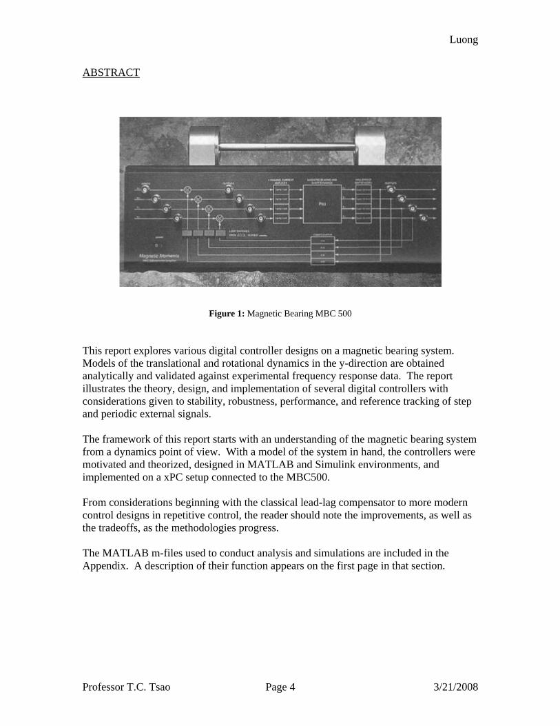
Figure 1: Magnetic Bearing MBC 500 This report explores various digital controller designs on a magnetic bearing system. Models of the translational and rotational dynamics in the y-direction are obtained analytically and validated against experimental frequency response data. The report illustrates the theory, design, and implementation of several digital controllers with considerations given to stability, robustness, performance, and reference tracking of step and periodic external signals. The framework of this report starts with an understanding of the magnetic bearing system from a dynamics point of view. With a model of the system in hand, the controllers were motivated and theorized, designed in MATLAB and Simulink environments, and implemented on a xPC setup connected to the MBC500. From considerations beginning with the classical lead-lag compensator to more modern control designs in repetitive control, the reader should note the improvements, as well as the tradeoffs, as the methodologies progress. The MATLAB m-files used to conduct analysis and simulations are included in the Appendix. A description of their function appears on the first page in that section.
Luong
Professor T.C. Tsao Page 5 3/21/2008
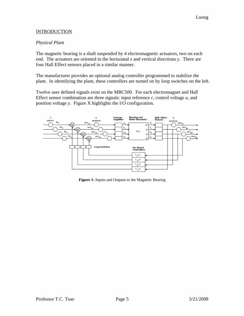
INTRODUCTION Physical Plant The magnetic bearing is a shaft suspended by 4 electromagnetic actuators, two on each end. The actuators are oriented in the horizontal x and vertical directions y. There are four Hall Effect sensors placed in a similar manner. The manufacturer provides an optional analog controller programmed to stabilize the plant. In identifying the plant, these controllers are turned on by loop switches on the left. Twelve user defined signals exist on the MBC500. For each electromagnet and Hall Effect sensor combination are three signals: input reference r, control voltage u, and position voltage y. Figure X highlights the I/O configuration.
Figure 1: Inputs and Outputs to the Magnetic Bearing
Luong
Professor T.C. Tsao Page 6 3/21/2008
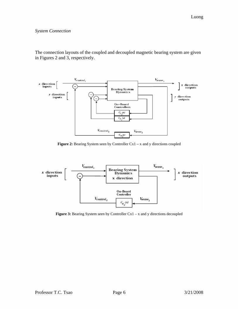
System Connection The connection layouts of the coupled and decoupled magnetic bearing system are given in Figures 2 and 3, respectively.
Figure 2: Bearing System seen by Controller Cx1 – x and y directions coupled
Figure 3: Bearing System seen by Controller Cx1 – x and y directions decoupled
Luong
Professor T.C. Tsao Page 7 3/21/2008
ANALYTICAL MODELING The modeling of the magnetic bearing is performed separately on the plant and the controller. The signal flow for the plant is D/A Voltage Amplifier Current Electromagnets Force Mechanical Dynamics Motion Sensor Voltage A/D
And the signal flow for the controller is
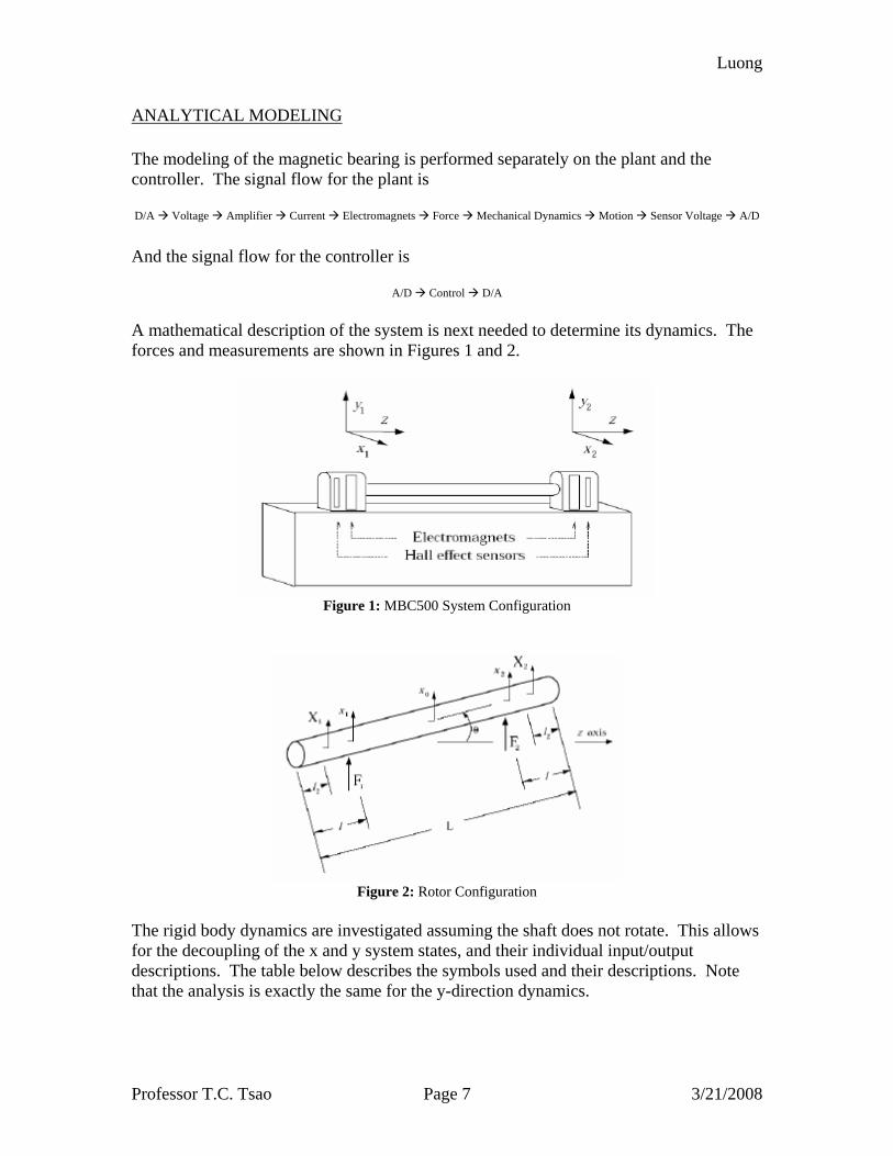
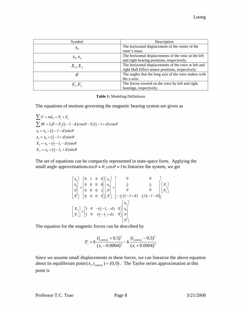
A/D Control D/A A mathematical description of the system is next needed to determine its dynamics. The forces and measurements are shown in Figures 1 and 2.
Figure 1: MBC500 System Configuration
Figure 2: Rotor Configuration
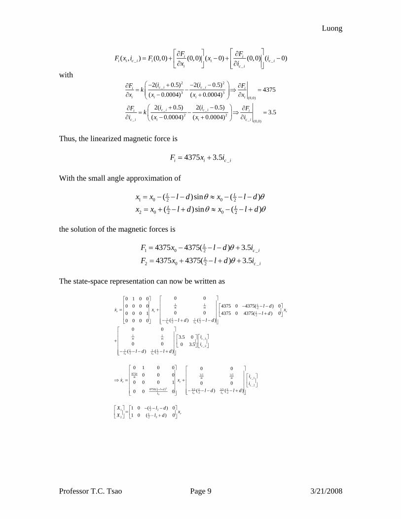
The rigid body dynamics are investigated assuming the shaft does not rotate. This allows for the decoupling of the x and y system states, and their individual input/output descriptions. The table below describes the symbols used and their descriptions. Note that the analysis is exactly the same for the y-direction dynamics.
Luong
Professor T.C. Tsao Page 8 3/21/2008
Symbol Description
0x The horizontal displacement of the center of the rotor’s mass.
1 2,x x The horizontal displacements of the rotor at the left and right bearing positions, respectively.
1 2,X X The horizontal displacements of the rotor at left and right Hall Effect sensor positions, respectively.
θ The angles that the long axis of the rotor makes with the z-axis.
1 2,F F The forces exerted on the rotor by left and right bearings, respectively.
Table 1: Modeling Definitions
The equations of motions governing the magnetic bearing system are given as
0 1 2
0 2 12 2
1 0 2
2 0 2
1 0 22
2 0 22
( ) cos ( ) cos
( )sin( )sin( )sin( )sin
L L
L
L
L
L
F mx F F
M I F l d F l d
x x l dx x l dX x l dX x l d
θ θ θ
θθθθ
= = +
= = − − − − +
= − − −
= + − +
= − − −
= + − +
∑∑
The set of equations can be compactly represented in state-space form. Applying the small angle approximationssin , cos 1θ θ θ≈ ≈ to linearize the system, we get
0 0
0 01 1
10 0
21 1
2 2
0
21 02
22 2
0 00 1 0 00 0 0 0
0 00 0 0 1( ) ( )0 0 0 0
1 0 ( ) 01 0 ( ) 0
m m
L LI I
L
L
x xFx xF
l d l d
xl dX x
l dX
θ θθ θ
θθ
⎡ ⎤⎡ ⎤ ⎡ ⎤ ⎡ ⎤⎢ ⎥⎢ ⎥ ⎢ ⎥ ⎢ ⎥ ⎡ ⎤⎢ ⎥⎢ ⎥ ⎢ ⎥ ⎢ ⎥= + ⎢ ⎥⎢ ⎥⎢ ⎥ ⎢ ⎥ ⎢ ⎥ ⎣ ⎦⎢ ⎥⎢ ⎥ ⎢ ⎥ ⎢ ⎥ − − + − −⎢ ⎥⎣ ⎦ ⎣ ⎦ ⎣ ⎦ ⎣ ⎦
⎡ ⎤⎢ ⎥− − −⎡ ⎤⎡ ⎤ ⎢ ⎥= ⎢ ⎥⎢ ⎥ ⎢ ⎥− +⎣ ⎦ ⎣ ⎦⎢ ⎥⎣ ⎦
The equation for the magnetic forces can be described by
2 2
2 2
( 0.5) ( 0.5)( 0.0004) ( 0.0004)
i icontrol controli
i i
i iF k k
x x+ −
= −− +
Since we assume small displacements in these forces, we can linearize the above equation about its equilibrium point ( , ) (0,0)
ii controlx i = . The Taylor series approximation at this point is
Luong
Professor T.C. Tsao Page 9 3/21/2008
_ __
( , ) (0,0) (0,0) ( 0) (0,0) ( 0)i ii i c i i i c i
i c i
F FF x i F x ix i
⎡ ⎤⎡ ⎤∂ ∂= + − + −⎢ ⎥⎢ ⎥∂ ∂⎢ ⎥⎣ ⎦ ⎣ ⎦
with 2 2
_ _3 3
(0,0)
_ _2 2
_ _ (0,0)
2( 0.5) 2( 0.5)4375
( 0.0004) ( 0.0004)
2( 0.5) 2( 0.5)3.5
( 0.0004) ( 0.0004)
c i c ii i
i i i i
c i c ii i
c i i i c i
i iF Fkx x x x
i iF Fki x x i
⎛ ⎞− + − −∂ ∂= − ⇒ =⎜ ⎟⎜ ⎟∂ − + ∂⎝ ⎠
+ −⎛ ⎞∂ ∂= − ⇒ =⎜ ⎟∂ − + ∂⎝ ⎠
Thus, the linearized magnetic force is
_4375 3.5i i c iF x i= + With the small angle approximation of
1 0 02 2
2 0 02 2
( )sin ( )( )sin ( )
L L
L L
x x l d x l dx x l d x l d
θ θθ θ
= − − − ≈ − − −
= + − + ≈ − − +
the solution of the magnetic forces is
1 0 _2
2 0 _2
4375 4375( ) 3.5
4375 4375( ) 3.5
Lc i
Lc i
F x l d i
F x l d i
θ
θ
= − − − +
= + − + +
The state-space representation can now be written as
0 0
0 0
1 12
21 1
2 2
1 1_1
_ 21 1
2 2
0 00 1 0 04375 0 4375( ) 00 0 0 0
0 0 4375 0 4375( ) 00 0 0 1( ) ( )0 0 0 0
0 03.5 0
0 0 0 3.5( ) ( )
Lm m
r r rL
L LI I
m m c
cL L
I I
l dx x x
l dl d l d
ii
l d l d
⎡ ⎤⎡ ⎤⎢ ⎥⎢ ⎥ − − −⎡ ⎤⎢ ⎥⎢ ⎥= + ⎢ ⎥⎢ ⎥⎢ ⎥ − +⎣ ⎦⎢ ⎥⎢ ⎥ − − + − −⎢ ⎥⎣ ⎦ ⎣ ⎦
⎡ ⎤⎢ ⎥ ⎡ ⎤⎡ ⎤⎢ ⎥+ ⎢ ⎥⎢ ⎥⎢ ⎥ ⎣ ⎦ ⎣ ⎦⎢ ⎥− − − − +⎢ ⎥⎣ ⎦
⇒2
20 00
8750 3.5 3.5_1
_ 28750( ) 3.5 3.5
2 2
21 2
22 2
0 1 0 0 0 00 0 0
0 0 0 1 0 0( ) ( )0 0 0
1 0 ( ) 01 0 ( ) 0
L
m m m cr r
cl d L L
I II
L
rL
ix x
il d l d
l dXx
l dX
− +
⎡ ⎤ ⎡ ⎤⎢ ⎥ ⎢ ⎥ ⎡ ⎤⎢ ⎥ ⎢ ⎥= + ⎢ ⎥⎢ ⎥ ⎢ ⎥ ⎣ ⎦⎢ ⎥ ⎢ ⎥− − − − +⎢ ⎥ ⎢ ⎥⎣ ⎦⎣ ⎦
− − −⎡ ⎤⎡ ⎤= ⎢ ⎥⎢ ⎥ − +⎣ ⎦ ⎣ ⎦
Luong
Professor T.C. Tsao Page 10 3/21/2008
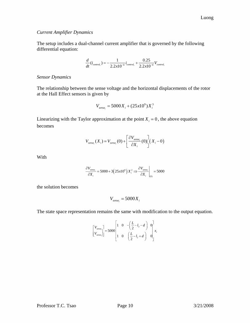
Current Amplifier Dynamics The setup includes a dual-channel current amplifier that is governed by the following differential equation:
4 4
1 0.25( )2.2 10 2.2 10i i icontrol control control
d i i Vdt x x− −= − +
Sensor Dynamics The relationship between the sense voltage and the horizontal displacements of the rotor at the Hall Effect sensors is given by
9 35000 (25 10 )isense i iV X x X= +
Linearizing with the Taylor approximation at the point 0iX = , the above equation becomes
( )( ) (0) (0) 0i
i i
sensesense i sense i
i
VV X V X
X∂⎡ ⎤
= + −⎢ ⎥∂⎣ ⎦
With
( )9 2
(0)
5000 3 25 10 5000i isense sensei
i i
V Vx X
X X∂ ∂
= + ⇒ =∂ ∂
the solution becomes
5000isense iV X=
The state space representation remains the same with modification to the output equation.
1
2
2
2
1 0 02
50001 0 0
2
senser
sense
L l dVx
V L l d
⎡ ⎤⎛ ⎞− − −⎜ ⎟⎢ ⎥⎡ ⎤ ⎝ ⎠⎢ ⎥=⎢ ⎥⎢ ⎥⎛ ⎞⎢ ⎥⎣ ⎦ − +⎢ ⎥⎜ ⎟
⎝ ⎠⎣ ⎦
Luong
Professor T.C. Tsao Page 11 3/21/2008
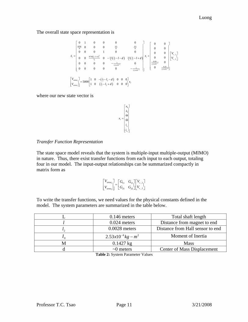
The overall state space representation is
( ) ( ) ( )2
2
0 0 0
44
44
8750 3.5 3.5
_18750 1 3.5 3.5
_ 22 20.25
12.2 10
2.2 100.25
12.2 10
2.2 10
0 1 0 0 0 0 0 00 0 0 0 0
0 0 0 1 0 0 0 00 00 0 0
00 0 0 0 000 0 0 0 0
L
m m m
cdr rL L
cI I I
xx
xx
sense
Vx x
Vl d l d
V
−−
−−
− +
⎡ ⎤ ⎡ ⎤⎢ ⎥ ⎢ ⎥⎢ ⎥ ⎢ ⎥⎢ ⎥ ⎢ ⎥ ⎡ ⎤⎢ ⎥ ⎢ ⎥= + ⎢ ⎥⎢ ⎥− − − − + ⎢ ⎥ ⎣ ⎦⎢ ⎥ ⎢ ⎥−⎢ ⎥ ⎢ ⎥⎢ ⎥ ⎢ ⎥− ⎣ ⎦⎢ ⎥⎣ ⎦
( )( )
1
2
22
22
1 0 0 0 05000
1 0 0 0 0
L
rLsense
l dx
l dV⎡ ⎤ ⎡ ⎤− − −
=⎢ ⎥ ⎢ ⎥− +⎢ ⎥ ⎣ ⎦⎣ ⎦
where our new state vector is
1
2
0
0
r
c
c
xx
x
i
i
⎡ ⎤⎢ ⎥⎢ ⎥⎢ ⎥Θ
= ⎢ ⎥Θ⎢ ⎥⎢ ⎥⎢ ⎥⎢ ⎥⎣ ⎦
Transfer Function Representation The state space model reveals that the system is multiple-input multiple-output (MIMO) in nature. Thus, there exist transfer functions from each input to each output, totaling four in our model. The input-output relationships can be summarized compactly in matrix form as
1
2
_111 12
_ 221 22
sense c
csense
V VG GVG GV
⎡ ⎤ ⎡ ⎤⎡ ⎤=⎢ ⎥ ⎢ ⎥⎢ ⎥
⎢ ⎥ ⎣ ⎦ ⎣ ⎦⎣ ⎦
To write the transfer functions, we need values for the physical constants defined in the model. The system parameters are summarized in the table below.
L 0.146 meters Total shaft length l 0.024 meters Distance from magnet to end 2l 0.0028 meters Distance from Hall sensor to end
0I 4 22.53 10x kg m− − Moment of Inertia M 0.1427 kg Mass d ~0 meters Center of Mass Displacement
Table 2: System Parameter Values
Luong
Professor T.C. Tsao Page 12 3/21/2008
With these parameter values, the corresponding state space representation is then
( ) ( ) ( )2
2
0 0 0
44
44
1
8750 3.5 3.5
_18750 1 3.5 3.5
_ 22 20.25
12.2 10
2.2 100.25
1 2.2 102.2 10
0 1 0 0 0 0 0 00 0 0 0 0
0 0 0 1 0 0 0 00 00 0 0
00 0 0 0 000 0 0 0 0
L
m m m
cr rL L
cI I I
xx
xx
sense
sens
Vx x
Vl l
V
V
−−
−−
−
⎡ ⎤ ⎡ ⎤⎢ ⎥ ⎢ ⎥⎢ ⎥ ⎢ ⎥⎢ ⎥ ⎢ ⎥ ⎡ ⎤⎢ ⎥ ⎢ ⎥= + ⎢ ⎥⎢ ⎥− − − ⎢ ⎥ ⎣ ⎦⎢ ⎥ ⎢ ⎥−⎢ ⎥ ⎢ ⎥⎢ ⎥ ⎢ ⎥− ⎣ ⎦⎢ ⎥⎣ ⎦
( )( )
2
22
22
1 0 0 0 05000
1 0 0 0 0
L
rLe
l dx
l d⎡ ⎤ ⎡ ⎤− − −
=⎢ ⎥ ⎢ ⎥− +⎢ ⎥ ⎣ ⎦⎣ ⎦
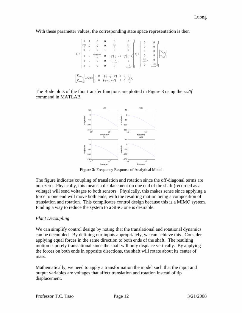
The Bode plots of the four transfer functions are plotted in Figure 3 using the ss2tf command in MATLAB.
102 104-150
-100
-50
0
50
frequency
mag
nitu
de
G11
102 104-150
-100
-50
0
50
frequency
mag
nitu
de
G12
102 104-150
-100
-50
0
50
frequency
mag
nitu
de
G21
102 104-150
-100
-50
0
50
frequency
mag
nitu
de
G22
Figure 3: Frequency Response of Analytical Model
The figure indicates coupling of translation and rotation since the off-diagonal terms are non-zero. Physically, this means a displacement on one end of the shaft (recorded as a voltage) will send voltages to both sensors. Physically, this makes sense since applying a force to one end will move both ends, with the resulting motion being a composition of translation and rotation. This complicates control design because this is a MIMO system. Finding a way to reduce the system to a SISO one is desirable. Plant Decoupling We can simplify control design by noting that the translational and rotational dynamics can be decoupled. By defining our inputs appropriately, we can achieve this. Consider applying equal forces in the same direction to both ends of the shaft. The resulting motion is purely translational since the shaft will only displace vertically. By applying the forces on both ends in opposite directions, the shaft will rotate about its center of mass. Mathematically, we need to apply a transformation the model such that the input and output variables are voltages that affect translation and rotation instead of tip displacement.
Luong
Professor T.C. Tsao Page 13 3/21/2008
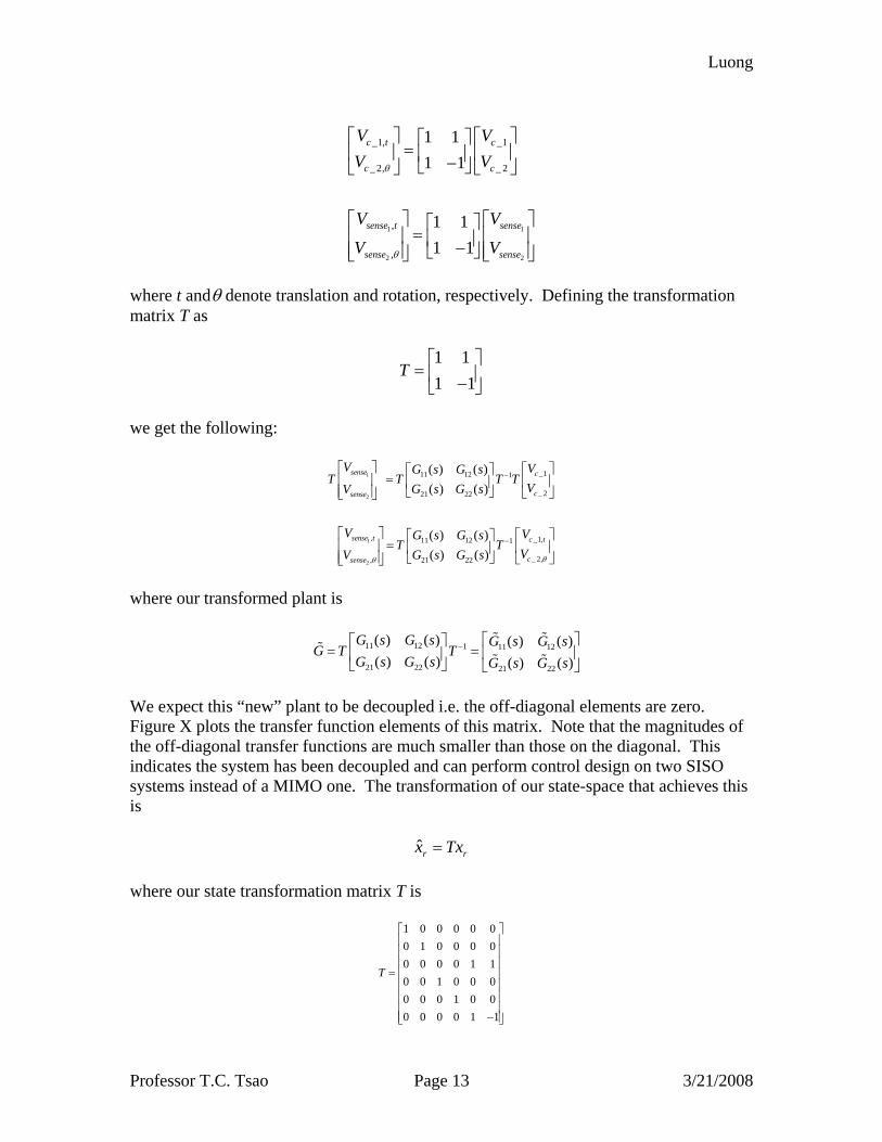
1 1
2 2
_1, _1
_ 2, _ 2
,
,
1 11 1
1 11 1
c t c
c c
sense t sense
sense sense
V VV V
V V
V V
θ
θ
⎡ ⎤ ⎡ ⎤⎡ ⎤=⎢ ⎥ ⎢ ⎥⎢ ⎥−⎣ ⎦⎣ ⎦ ⎣ ⎦
⎡ ⎤ ⎡ ⎤⎡ ⎤=⎢ ⎥ ⎢ ⎥⎢ ⎥−⎣ ⎦⎢ ⎥ ⎢ ⎥⎣ ⎦ ⎣ ⎦
where t andθ denote translation and rotation, respectively. Defining the transformation matrix T as
1 11 1
T⎡ ⎤
= ⎢ ⎥−⎣ ⎦
we get the following:
1
2
1
2
_111 12 1
_ 221 22
, _1,11 12 1
_ 2,21 22,
( ) ( )( ) ( )
( ) ( )( ) ( )
sense c
csense
sense t c t
csense
V VG s G sT T T T
VG s G sV
V VG s G sT T
VG s G sV θθ
−
−
⎡ ⎤ ⎡ ⎤⎡ ⎤=⎢ ⎥ ⎢ ⎥⎢ ⎥
⎢ ⎥ ⎣ ⎦ ⎣ ⎦⎣ ⎦
⎡ ⎤ ⎡ ⎤⎡ ⎤=⎢ ⎥ ⎢ ⎥⎢ ⎥
⎢ ⎥ ⎣ ⎦ ⎣ ⎦⎣ ⎦
where our transformed plant is
11 12 1 11 12
21 22 21 22
( ) ( ) ( ) ( )( ) ( ) ( ) ( )
G s G s G s G sG T T
G s G s G s G s− ⎡ ⎤⎡ ⎤
= = ⎢ ⎥⎢ ⎥⎣ ⎦ ⎣ ⎦
We expect this “new” plant to be decoupled i.e. the off-diagonal elements are zero. Figure X plots the transfer function elements of this matrix. Note that the magnitudes of the off-diagonal transfer functions are much smaller than those on the diagonal. This indicates the system has been decoupled and can perform control design on two SISO systems instead of a MIMO one. The transformation of our state-space that achieves this is
ˆr rx Tx=
where our state transformation matrix T is
1 0 0 0 0 00 1 0 0 0 00 0 0 0 1 10 0 1 0 0 00 0 0 1 0 00 0 0 0 1 1
T
⎡ ⎤⎢ ⎥⎢ ⎥⎢ ⎥
= ⎢ ⎥⎢ ⎥⎢ ⎥⎢ ⎥
−⎢ ⎥⎣ ⎦
Luong
Professor T.C. Tsao Page 14 3/21/2008
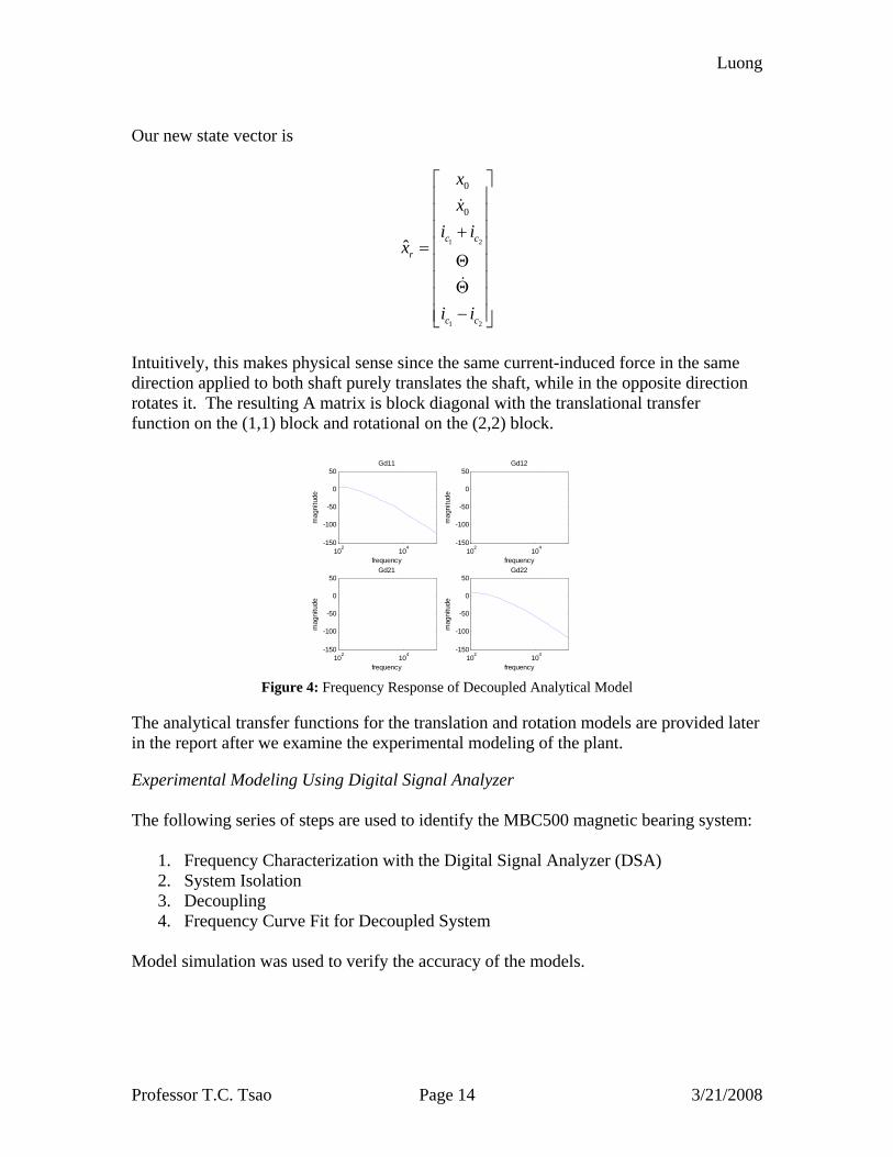
Our new state vector is
1 2
1 2
0
0
ˆ c cr
c c
xx
i ix
i i
⎡ ⎤⎢ ⎥⎢ ⎥⎢ ⎥+
= ⎢ ⎥Θ⎢ ⎥
⎢ ⎥Θ⎢ ⎥
−⎢ ⎥⎣ ⎦
Intuitively, this makes physical sense since the same current-induced force in the same direction applied to both shaft purely translates the shaft, while in the opposite direction rotates it. The resulting A matrix is block diagonal with the translational transfer function on the (1,1) block and rotational on the (2,2) block.
102 104-150
-100
-50
0
50
frequency
mag
nitu
de
Gd11
102 104-150
-100
-50
0
50
frequency
mag
nitu
de
Gd12
102 104-150
-100
-50
0
50
frequency
mag
nitu
de
Gd21
102 104-150
-100
-50
0
50
frequency
mag
nitu
de
Gd22
Figure 4: Frequency Response of Decoupled Analytical Model
The analytical transfer functions for the translation and rotation models are provided later in the report after we examine the experimental modeling of the plant. Experimental Modeling Using Digital Signal Analyzer The following series of steps are used to identify the MBC500 magnetic bearing system:
1. Frequency Characterization with the Digital Signal Analyzer (DSA) 2. System Isolation 3. Decoupling 4. Frequency Curve Fit for Decoupled System
Model simulation was used to verify the accuracy of the models.
Luong
Professor T.C. Tsao Page 15 3/21/2008
Frequency Characterization The coupling between the horizontal and vertical directions is ignored in the characterization. When the characterization is performed between directions, the signal is very small. However, the positions are extremely coupled when taken in the same direction. The 2x2 system must be considered as a whole. For simplicity, the analysis will consider only one direction, and can be repeated for the other. The control signal u cannot be directly controlled, so we circumvent this fact by finding the transfer function between r and u in addition to r to y. Using the DSA, we refer to transfer functions as ruT and ryT , respectively. Classical linear feedback control theory tells us that
( ) 1
1(1 )ru
ry
T I CG
T CG G
−
−
= +
= +
With all the combinations between sides, eight frequency responses are obtained
1 1 1 1r u r yT withT 1 2 1 2r u r yT withT
2 1 2 1r u r yT withT 2 2 2 2r u r yT withT
System Isolation We know that
ry
ru
Y T R
U T R
=
=
Combining the two, we get
1ry ruY T T U−=
The system plant from input u to output y is then defined as
11 1 1 2 1 1 1 211 12
2 1 2 2 2 1 2 221 22
r y r y r u r u
r y r y r u r u
T T T TG GG
T T T TG G
−⎡ ⎤ ⎡ ⎤⎡ ⎤
= = =⎢ ⎥ ⎢ ⎥⎢ ⎥⎣ ⎦ ⎣ ⎦⎣ ⎦
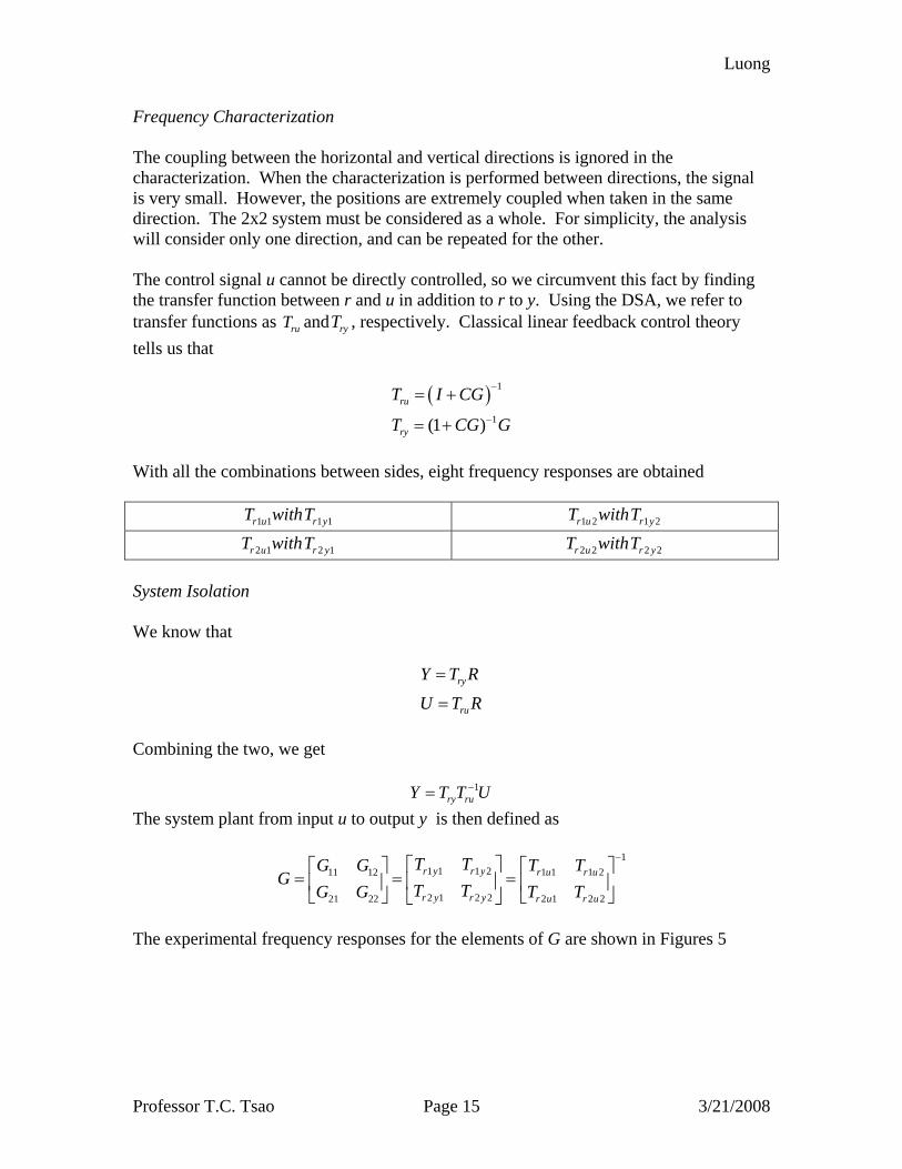
The experimental frequency responses for the elements of G are shown in Figures 5
Luong
Professor T.C. Tsao Page 16 3/21/2008
2 4 6 8 10-60
-40
-20
0
20Gy11
Frequency (Hz)
Mag
nitu
de (d
B)
2 4 6 8 10-80
-60
-40
-20
0Gy12
Frequency (Hz)
Mag
nitu
de (d
B)
2 4 6 8 10-80
-60
-40
-20
0Gy21
Frequency (Hz)M
agni
tude
(dB
)2 4 6 8 10
-100
-50
0
50Gy22
Frequency (Hz)
Mag
nitu
de (d
B)
Figure 5: Frequency Response of Physical System
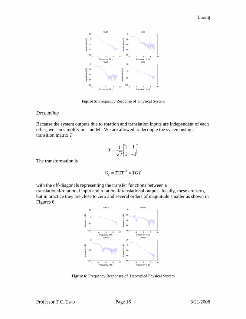
Decoupling Because the system outputs due to rotation and translation inputs are independent of each other, we can simplify our model. We are allowed to decouple the system using a transition matrix T
1 111 12
T⎡ ⎤
= ⎢ ⎥−⎣ ⎦
The transformation is
1dG TGT TGT−= =
with the off-diagonals representing the transfer functions between a translational/rotational input and rotational/translational output. Ideally, these are zero, but in practice they are close to zero and several orders of magnitude smaller as shown in Figures 6.
2 4 6 8 10-100
-50
0
50Gdy11
Frequency (Hz)
Mag
nitu
de (d
B)
2 4 6 8 10-80
-60
-40
-20
0Gdy12
Frequency (Hz)
Mag
nitu
de (d
B)
2 4 6 8 10-100
-50
0Gdy21
Frequency (Hz)
Mag
nitu
de (d
B)
2 4 6 8 10-60
-40
-20
0
20Gdy22
Frequency (Hz)
Mag
nitu
de (d
B)
Figure 6: Frequency Responses of Decoupled Physical System
Luong
Professor T.C. Tsao Page 17 3/21/2008
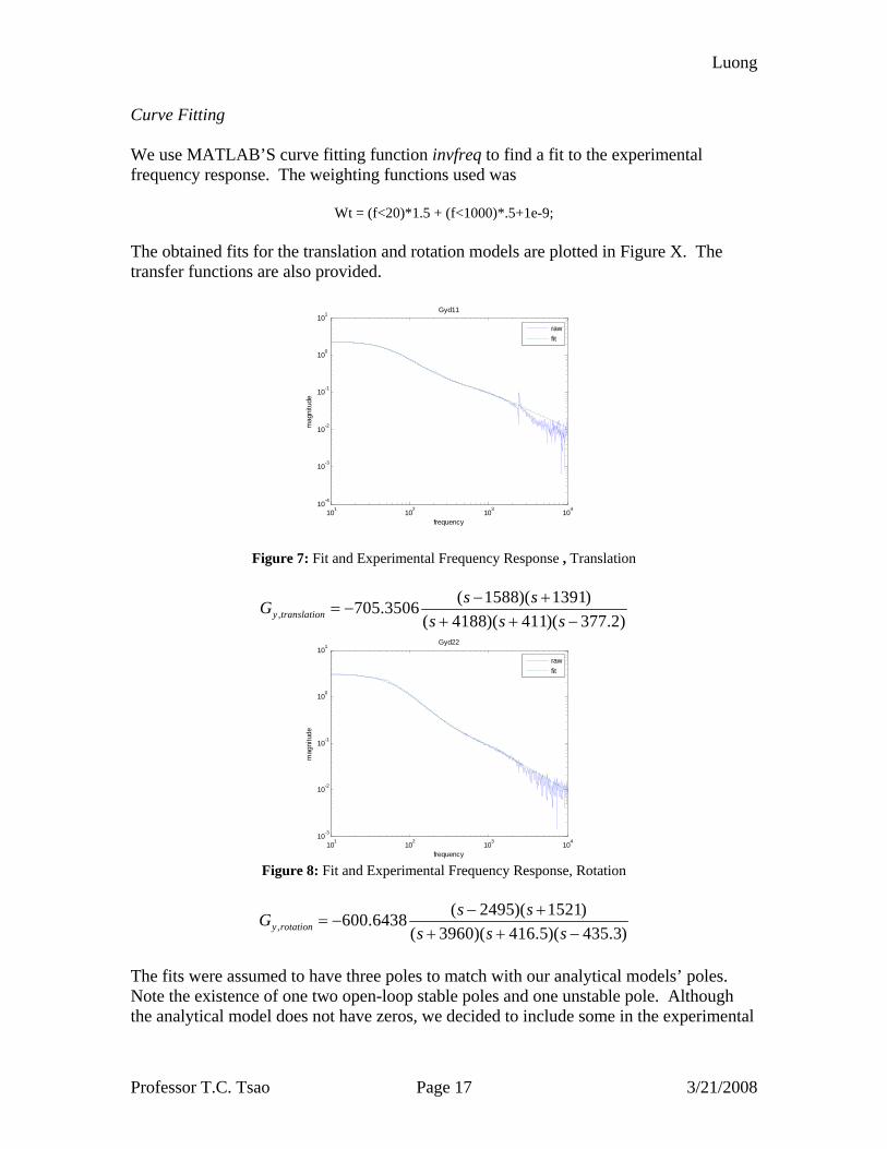
Curve Fitting We use MATLAB’S curve fitting function invfreq to find a fit to the experimental frequency response. The weighting functions used was
Wt = (f<20)*1.5 + (f<1000)*.5+1e-9;
The obtained fits for the translation and rotation models are plotted in Figure X. The transfer functions are also provided.
101 102 103 10410-4
10-3
10-2
10-1
100
101
frequency
mag
nitu
deGyd11
rawfit
Figure 7: Fit and Experimental Frequency Response , Translation
,( 1588)( 1391)705.3506
( 4188)( 411)( 377.2)y translations sG
s s s− +
= −+ + −
101 102 103 10410-3
10-2
10-1
100
101
frequency
mag
nitu
de
Gyd22
rawfit
Figure 8: Fit and Experimental Frequency Response, Rotation
,( 2495)( 1521)600.6438
( 3960)( 416.5)( 435.3)y rotations sG
s s s− +
= −+ + −
The fits were assumed to have three poles to match with our analytical models’ poles. Note the existence of one two open-loop stable poles and one unstable pole. Although the analytical model does not have zeros, we decided to include some in the experimental
Luong
Professor T.C. Tsao Page 18 3/21/2008
model to increase the goodness of fit. We will use the experimental models to design controllers.
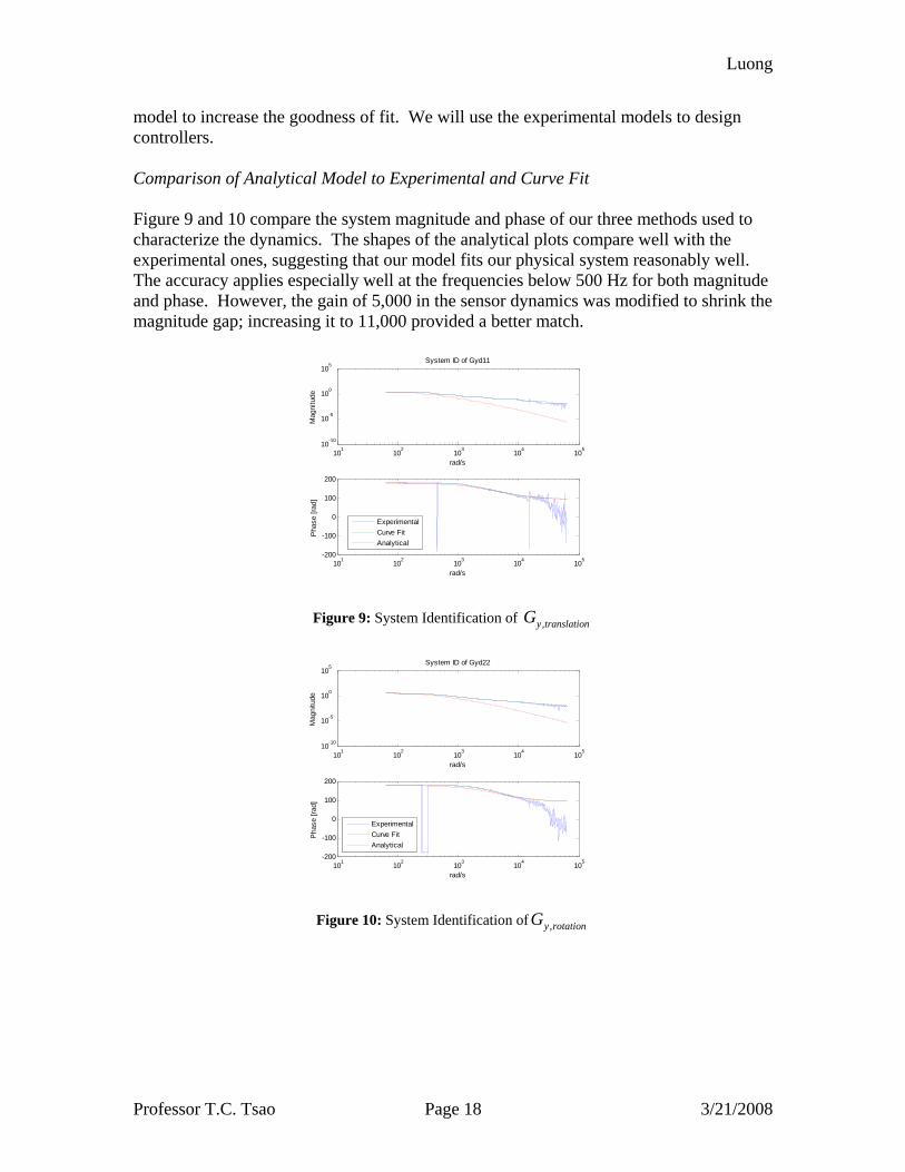
Comparison of Analytical Model to Experimental and Curve Fit Figure 9 and 10 compare the system magnitude and phase of our three methods used to characterize the dynamics. The shapes of the analytical plots compare well with the experimental ones, suggesting that our model fits our physical system reasonably well. The accuracy applies especially well at the frequencies below 500 Hz for both magnitude and phase. However, the gain of 5,000 in the sensor dynamics was modified to shrink the magnitude gap; increasing it to 11,000 provided a better match.
101 102 103 104 10510-10
10-5
100
105System ID of Gyd11
rad/s
Mag
nitu
de
101 102 103 104 105-200
-100
0
100
200
rad/s
Pha
se [r
ad]
ExperimentalCurve FitAnalytical
Figure 9: System Identification of ,y translationG
101 102 103 104 10510-10
10-5
100
105System ID of Gyd22
rad/s
Mag
nitu
de
101 102 103 104 105-200
-100
0
100
200
rad/s
Pha
se [r
ad]
ExperimentalCurve FitAnalytical
Figure 10: System Identification of ,y rotationG
Luong
Professor T.C. Tsao Page 19 3/21/2008
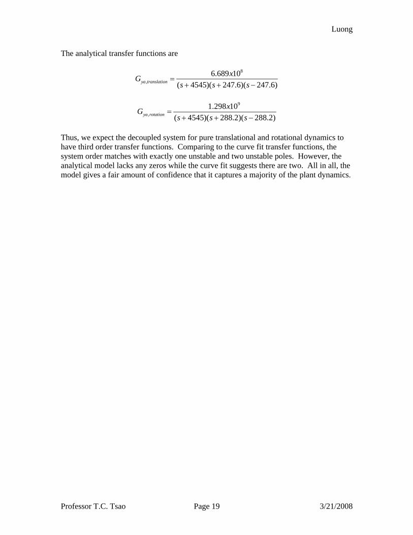
The analytical transfer functions are
8
,6.689 10
( 4545)( 247.6)( 247.6)ya translationxG
s s s=
+ + −
9
,1.298 10
( 4545)( 288.2)( 288.2)ya rotationxG
s s s=
+ + −
Thus, we expect the decoupled system for pure translational and rotational dynamics to have third order transfer functions. Comparing to the curve fit transfer functions, the system order matches with exactly one unstable and two unstable poles. However, the analytical model lacks any zeros while the curve fit suggests there are two. All in all, the model gives a fair amount of confidence that it captures a majority of the plant dynamics.

Luong
Professor T.C. Tsao Page 20 3/21/2008
CONTROLLER DESIGNS As a class, we will use the transfer functions of the translation and rotational of the plant in the y direction
2 5 9
, 3 2 4 8
681.1 1.843 10 1.553 10( )4075 4.024 10 6.537 10d translation
s sG ss s− + ⋅ + ⋅
=+ − ⋅ − ⋅
2 5 9
, 3 2 4 8
589.6 5.722 10 2.454 10( )4056 2.441 10 7.692 10d rotation
s sG ss s− + ⋅ + ⋅
=+ − ⋅ − ⋅
instead of the ones obtained in the analytical modeling and curve fit. They are both open loop unstable due to poles in the right half complex plane. It turns out that the transfer functions were very similar in form for the x-direction. Methodology Step 1: (G(s),C(s)) For each controller presented in this report, we design based on the low-order models for its simplicity. Step 2: (Gzoh(z),C(z)) We map the controller, if necessary, and the model of the plant into the z-domain for digital implementation via a zero-order hold function and a specified sampling time. Step 3: (Gactual,zoh(z), C(z): Simulation We expect the designed controller will stabilize the plant. Before implementing the controller, we run simulations on a higher order plant model to reduce the possibility for unstable compensation. For this, we use a 10th order model of the original (coupled) plant that we decouple as necessary to implement the translation and rotation controllers. Step 4: (Gactual(s) C(z)): Implementation We implement the controllers to the actual system, and compare the experimental results to the simulated ones for verification.
Luong
Professor T.C. Tsao Page 21 3/21/2008
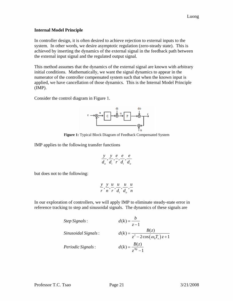
Internal Model Principle In controller design, it is often desired to achieve rejection to external inputs to the system. In other words, we desire asymptotic regulation (zero-steady state). This is achieved by inserting the dynamics of the external signal in the feedback path between the external input signal and the regulated output signal. This method assumes that the dynamics of the external signal are known with arbitrary initial conditions. Mathematically, we want the signal dynamics to appear in the numerator of the controller compensated system such that when the known input is applied, we have cancellation of those dynamics. This is the Internal Model Principle (IMP). Consider the control diagram in Figure 1.
Figure 1: Typical Block Diagram of Feedback Compensated System
IMP applies to the following transfer functions
, , , ,o i i o
y y e e ed d r d d
but does not to the following:
, , , , ,i o
y y u u u ur n r d d n
In our exploration of controllers, we will apply IMP to eliminate steady-state error in reference tracking to step and sinusoidal signals. The dynamics of these signals are
( )20
: ( )1
( ): ( )2cos 1
( ): ( )1
s
Np
bStep Signals d kz
B zSinusoidal Signals d kz T zB zPeriodic Signals d k
z
ω
=−
=− +
=−
Luong
Professor T.C. Tsao Page 22 3/21/2008
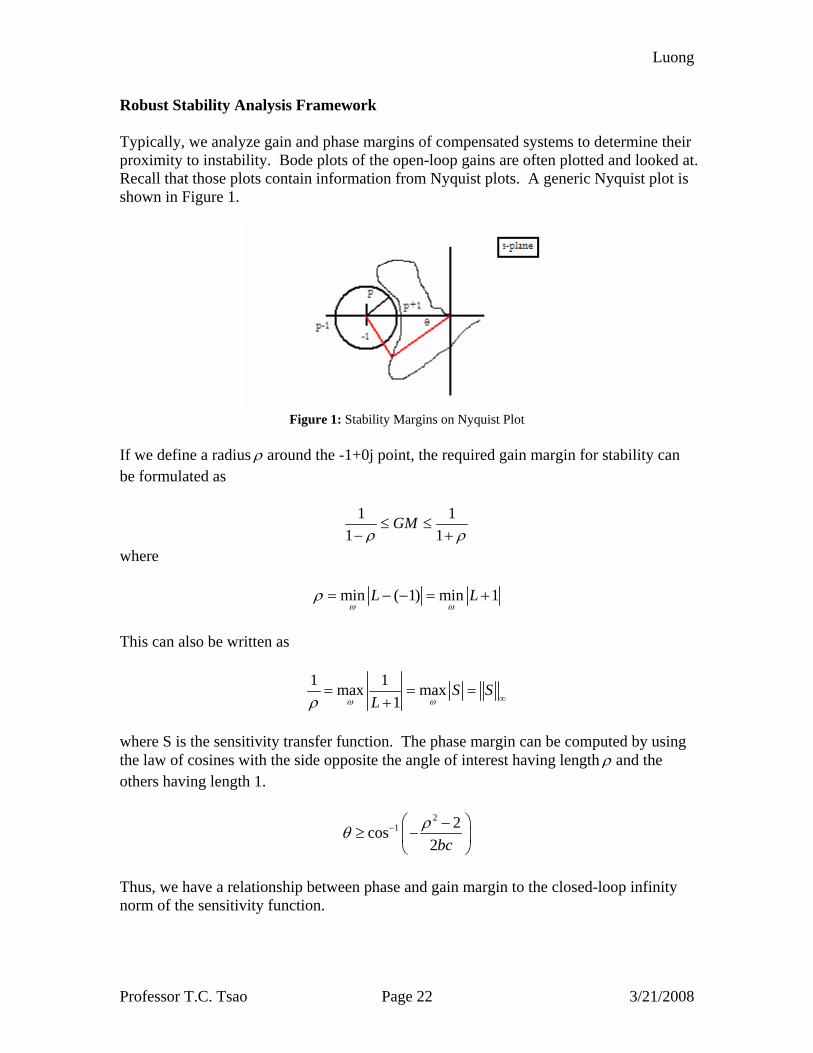
Robust Stability Analysis Framework Typically, we analyze gain and phase margins of compensated systems to determine their proximity to instability. Bode plots of the open-loop gains are often plotted and looked at. Recall that those plots contain information from Nyquist plots. A generic Nyquist plot is shown in Figure 1.
Figure 1: Stability Margins on Nyquist Plot
If we define a radius ρ around the -1+0j point, the required gain margin for stability can be formulated as
1 11 1
GMρ ρ≤ ≤
− +
where
min ( 1) min 1L Lω ω
ρ = − − = +
This can also be written as
1 1max max1
S SLω ωρ ∞
= = =+
where S is the sensitivity transfer function. The phase margin can be computed by using the law of cosines with the side opposite the angle of interest having length ρ and the others having length 1.
21 2cos
2bcρθ − ⎛ ⎞−
≥ −⎜ ⎟⎝ ⎠
Thus, we have a relationship between phase and gain margin to the closed-loop infinity norm of the sensitivity function.
Luong
Professor T.C. Tsao Page 23 3/21/2008
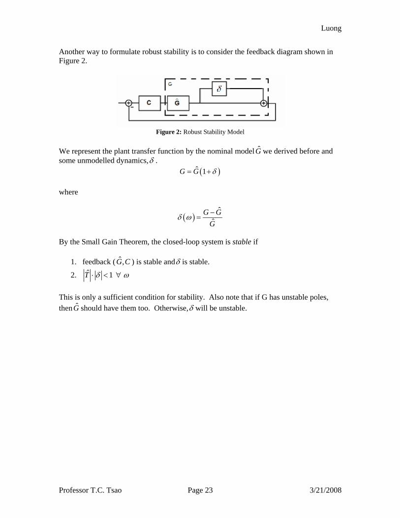
Another way to formulate robust stability is to consider the feedback diagram shown in Figure 2.
Figure 2: Robust Stability Model
We represent the plant transfer function by the nominal model G we derived before and some unmodelled dynamics,δ .
( )ˆ 1G G δ= + where
( )ˆ
ˆG G
Gδ ω −
=
By the Small Gain Theorem, the closed-loop system is stable if
1. feedback ( ˆ ,G C ) is stable andδ is stable.
2. ˆ 1T δ ω⋅ < ∀
This is only a sufficient condition for stability. Also note that if G has unstable poles, then G should have them too. Otherwise,δ will be unstable.
Luong
Professor T.C. Tsao Page 24 3/21/2008
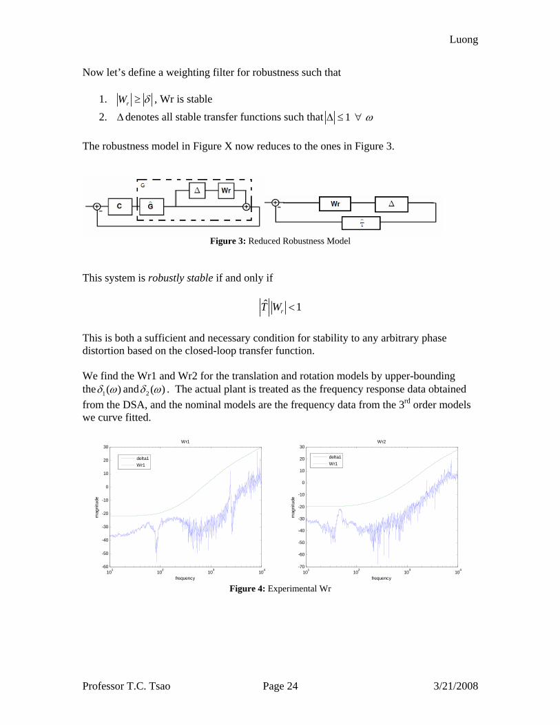
Now let’s define a weighting filter for robustness such that
1. rW δ≥ , Wr is stable 2. ∆denotes all stable transfer functions such that 1 ω∆ ≤ ∀
The robustness model in Figure X now reduces to the ones in Figure 3.
Figure 3: Reduced Robustness Model
This system is robustly stable if and only if
ˆ 1rT W <
This is both a sufficient and necessary condition for stability to any arbitrary phase distortion based on the closed-loop transfer function. We find the Wr1 and Wr2 for the translation and rotation models by upper-bounding the 1( )δ ω and 2 ( )δ ω . The actual plant is treated as the frequency response data obtained from the DSA, and the nominal models are the frequency data from the 3rd order models we curve fitted.
101 102 103 104-60
-50
-40
-30
-20
-10
0
10
20
30
frequency
mag
nitu
de
Wr1
delta1Wr1
101 102 103 104-70
-60
-50
-40
-30
-20
-10
0
10
20
30
frequency
mag
nitu
de
Wr2
delta1Wr1
Figure 4: Experimental Wr

Luong
Professor T.C. Tsao Page 25 3/21/2008
The transfer functions of the Wr’s are
( )( )
( )( )
031 4
042 4
2000 8005 10
105000 1000
4 102 10
s sWr
ss s
Wrs
−
−
+ += ⋅
++ +
= ⋅+ ⋅
We will design the controller C based on G such that ˆ1 0GC+ = is stable, i.e.
ˆˆˆ1
PCTPC
=+
is stable. Together with Wr, we are able to determine the stability robustness of each controller design. An important remark of this result is we desire the magnitude of T small for more robust stability. However, that would cause S to become larger and affect performance by decreasing the gain and phase margins. Thus, there is a tradeoff between robust stability and performance. At the expense of ensuring the compensated system is stable given modeling errors of the plant, performance is sacrificed.
Luong
Professor T.C. Tsao Page 26 3/21/2008
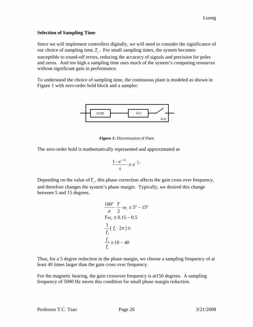
Selection of Sampling Time Since we will implement controllers digitally, we will need to consider the significance of our choice of sampling time, sT . For small sampling times, the system becomes susceptible to round-off errors, reducing the accuracy of signals and precision for poles and zeros. And too high a sampling time uses much of the system’s computing resources without significant gain in performance. To understand the choice of sampling time, the continuous plant is modeled as shown in Figure 1 with zero-order hold block and a sampler.
Figure 1: Discretization of Plant
The zero-order hold is mathematically represented and approximated as
21 s Ts
sTse e
s
−−−
≅
Depending on the value of sT , this phase correction affects the gain cross over frequency, and therefore changes the system’s phase margin. Typically, we desired this change between 5 and 15 degrees.
( )
180 5 1520.15 0.5
1 2
10 40
c
c
cs
s
c
T
T
ffff
ωπω
π
°⋅ ⋅ ≅ ° °
≅
⋅ ≅
≅
∼
∼
∼
Thus, for a 5 degree reduction in the phase margin, we choose a sampling frequency of at least 40 times larger than the gain cross over frequency. For the magnetic bearing, the gain crossover frequency is at150 degrees. A sampling frequency of 5000 Hz meets this condition for small phase margin reduction.
Luong
Professor T.C. Tsao Page 27 3/21/2008
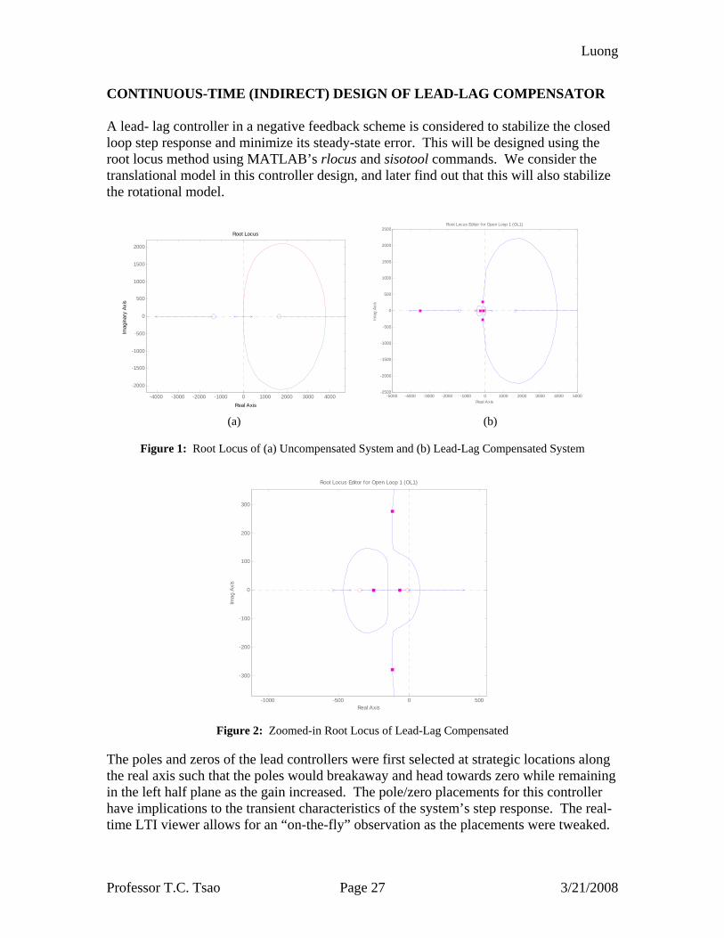
CONTINUOUS-TIME (INDIRECT) DESIGN OF LEAD-LAG COMPENSATOR A lead- lag controller in a negative feedback scheme is considered to stabilize the closed loop step response and minimize its steady-state error. This will be designed using the root locus method using MATLAB’s rlocus and sisotool commands. We consider the translational model in this controller design, and later find out that this will also stabilize the rotational model.
-4000 -3000 -2000 -1000 0 1000 2000 3000 4000
-2000
-1500
-1000
-500
0
500
1000
1500
2000
Root Locus
Real Axis
Imag
inar
y Ax
is
-5000 -4000 -3000 -2000 -1000 0 1000 2000 3000 4000 5000-2500
-2000
-1500
-1000
-500
0
500
1000
1500
2000
2500Root Locus Editor for Open Loop 1 (OL1)
Real Axis
Imag
Axi
s
(a) (b)
Figure 1: Root Locus of (a) Uncompensated System and (b) Lead-Lag Compensated System
-1000 -500 0 500
-300
-200
-100
0
100
200
300
Root Locus Editor for Open Loop 1 (OL1)
Real Axis
Imag
Axi
s
Figure 2: Zoomed-in Root Locus of Lead-Lag Compensated
The poles and zeros of the lead controllers were first selected at strategic locations along the real axis such that the poles would breakaway and head towards zero while remaining in the left half plane as the gain increased. The pole/zero placements for this controller have implications to the transient characteristics of the system’s step response. The real-time LTI viewer allows for an “on-the-fly” observation as the placements were tweaked.
Luong
Professor T.C. Tsao Page 28 3/21/2008
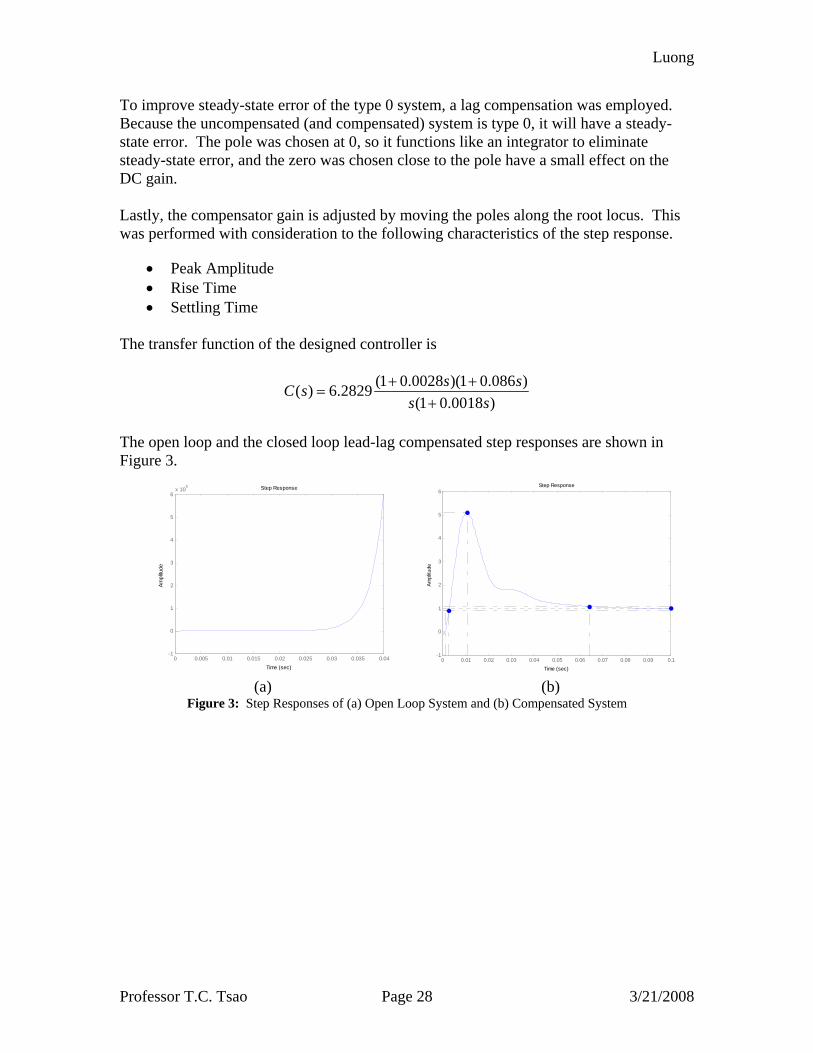
To improve steady-state error of the type 0 system, a lag compensation was employed. Because the uncompensated (and compensated) system is type 0, it will have a steady-state error. The pole was chosen at 0, so it functions like an integrator to eliminate steady-state error, and the zero was chosen close to the pole have a small effect on the DC gain. Lastly, the compensator gain is adjusted by moving the poles along the root locus. This was performed with consideration to the following characteristics of the step response.
• Peak Amplitude • Rise Time • Settling Time
The transfer function of the designed controller is
(1 0.0028 )(1 0.086 )( ) 6.2829(1 0.0018 )
s sC ss s
+ +=
+
The open loop and the closed loop lead-lag compensated step responses are shown in Figure 3.
0 0.005 0.01 0.015 0.02 0.025 0.03 0.035 0.04-1
0
1
2
3
4
5
6x 10
6 Step Response
Time (sec)
Ampl
itude
Step Response
Time (sec)
Ampl
itude
0 0.01 0.02 0.03 0.04 0.05 0.06 0.07 0.08 0.09 0.1-1
0
1
2
3
4
5
6
(a) (b)
Figure 3: Step Responses of (a) Open Loop System and (b) Compensated System
Luong
Professor T.C. Tsao Page 29 3/21/2008
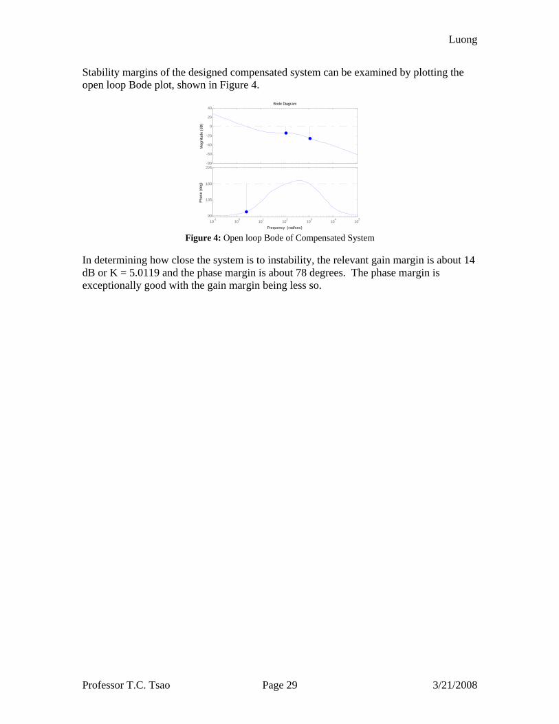
Stability margins of the designed compensated system can be examined by plotting the open loop Bode plot, shown in Figure 4.
Bode Diagram
Frequency (rad/sec)
-80
-60
-40
-20
0
20
40
Mag
nitu
de (d
B)
10-1
100
101
102
103
104
105
90
135
180
225
Phas
e (d
eg)
Figure 4: Open loop Bode of Compensated System
In determining how close the system is to instability, the relevant gain margin is about 14 dB or K = 5.0119 and the phase margin is about 78 degrees. The phase margin is exceptionally good with the gain margin being less so.
Luong
Professor T.C. Tsao Page 30 3/21/2008
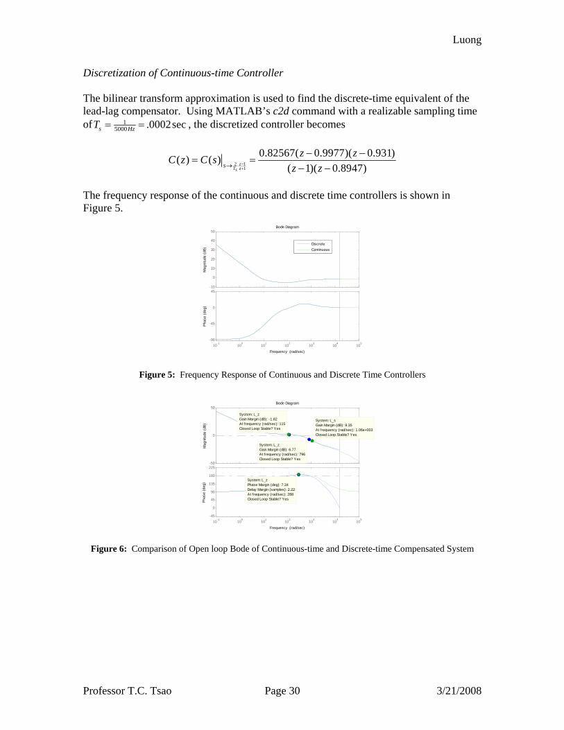
Discretization of Continuous-time Controller The bilinear transform approximation is used to find the discrete-time equivalent of the lead-lag compensator. Using MATLAB’s c2d command with a realizable sampling time of 1
5000 .0002secs HzT = = , the discretized controller becomes
2 11
0.82567( 0.9977)( 0.931)( ) ( )( 1)( 0.8947)z
T zss
z zC z C sz z−
+→
− −= =
− −
The frequency response of the continuous and discrete time controllers is shown in Figure 5.
-10
0
10
20
30
40
50
Mag
nitu
de (d
B)
10-1
100
101
102
103
104
105
-90
-45
0
45
Phas
e (d
eg)
Bode Diagram
Frequency (rad/sec)
DiscreteContinuous
Figure 5: Frequency Response of Continuous and Discrete Time Controllers
Bode Diagram
Frequency (rad/sec)10
-110
010
110
210
310
410
5-45
0
45
90
135
180
225
System: L_zPhase Margin (deg): 7.34Delay Margin (samples): 2.22At frequency (rad/sec): 288Closed Loop Stable? YesPh
ase
(deg
)
-50
0
50
System: L_sGain Margin (dB): 9.35At frequency (rad/sec): 1.06e+003Closed Loop Stable? Yes
System: L_zGain Margin (dB): 6.77At frequency (rad/sec): 796Closed Loop Stable? Yes
System: L_zGain Margin (dB): -1.82At frequency (rad/sec): 115Closed Loop Stable? Yes
Mag
nitu
de (d
B)
Figure 6: Comparison of Open loop Bode of Continuous-time and Discrete-time Compensated System

Luong
Professor T.C. Tsao Page 31 3/21/2008
The approximation begins to worsen significantly at sec800 rad for the phase plot. This frequency at which distortion becomes more significant may need to be larger depending on the frequency range of interest. Increasing the sampling time would make the adjustment. Note that the stability margins in the continuous-time system are almost identical to the ones in the discrete-time system. Thus, the indirect design of the controller, although an approximation at the discretization step, maintains the system stability characteristics, and should produce similar results in implementation as predicted in continuous-time design.
Luong
Professor T.C. Tsao Page 32 3/21/2008
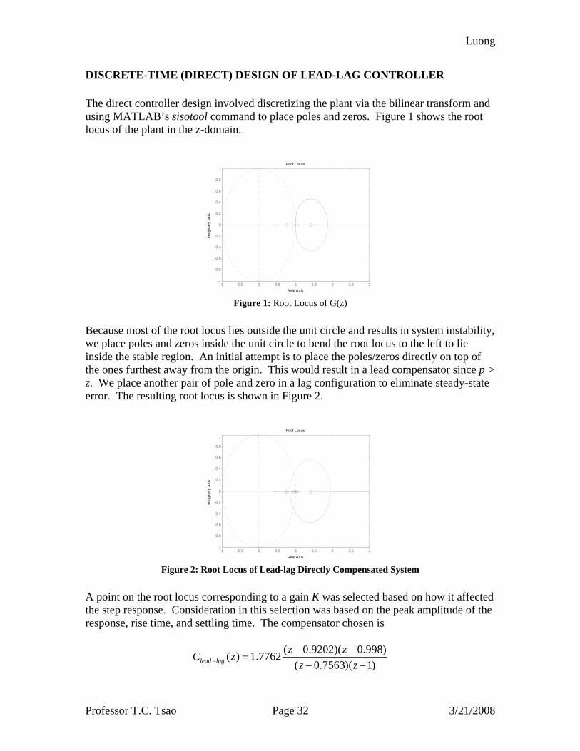
DISCRETE-TIME (DIRECT) DESIGN OF LEAD-LAG CONTROLLER The direct controller design involved discretizing the plant via the bilinear transform and using MATLAB’s sisotool command to place poles and zeros. Figure 1 shows the root locus of the plant in the z-domain.
-1 -0.5 0 0.5 1 1.5 2 2.5 3-1
-0.8
-0.6
-0.4
-0.2
0
0.2
0.4
0.6
0.8
1Root Locus
Real Axis
Imag
inar
y Ax
is
Figure 1: Root Locus of G(z)
Because most of the root locus lies outside the unit circle and results in system instability, we place poles and zeros inside the unit circle to bend the root locus to the left to lie inside the stable region. An initial attempt is to place the poles/zeros directly on top of the ones furthest away from the origin. This would result in a lead compensator since p > z. We place another pair of pole and zero in a lag configuration to eliminate steady-state error. The resulting root locus is shown in Figure 2.
-1 -0.5 0 0.5 1 1.5 2 2.5 3-1
-0.8
-0.6
-0.4
-0.2
0
0.2
0.4
0.6
0.8
1Root Locus
Real Axis
Imag
inar
y Ax
is
Figure 2: Root Locus of Lead-lag Directly Compensated System
A point on the root locus corresponding to a gain K was selected based on how it affected the step response. Consideration in this selection was based on the peak amplitude of the response, rise time, and settling time. The compensator chosen is
( 0.9202)( 0.998)( ) 1.7762
( 0.7563)( 1)lead lagz zC z
z z−
− −=
− −
Luong
Professor T.C. Tsao Page 33 3/21/2008
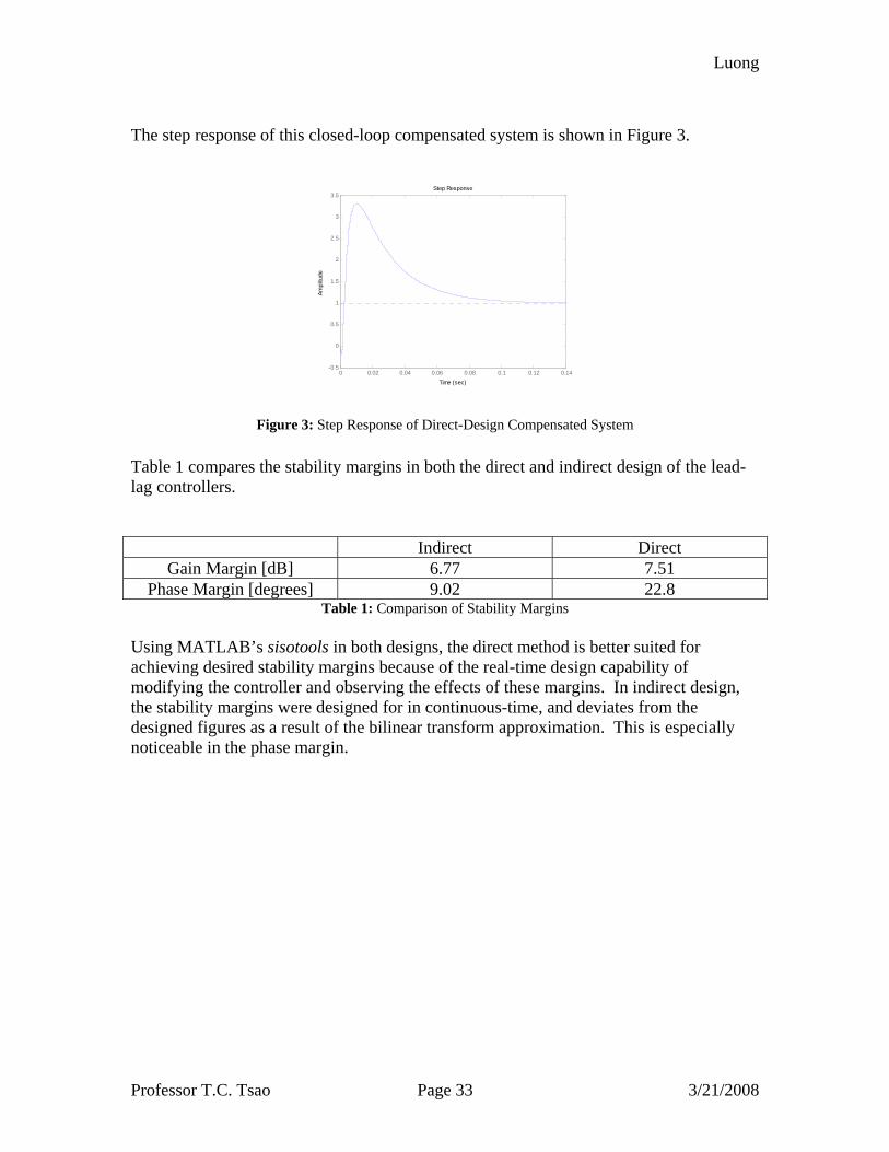
The step response of this closed-loop compensated system is shown in Figure 3.
0 0.02 0.04 0.06 0.08 0.1 0.12 0.14-0.5
0
0.5
1
1.5
2
2.5
3
3.5Step Response
Time (sec)
Ampl
itude
Figure 3: Step Response of Direct-Design Compensated System Table 1 compares the stability margins in both the direct and indirect design of the lead-lag controllers.
Indirect Direct Gain Margin [dB] 6.77 7.51
Phase Margin [degrees] 9.02 22.8 Table 1: Comparison of Stability Margins
Using MATLAB’s sisotools in both designs, the direct method is better suited for achieving desired stability margins because of the real-time design capability of modifying the controller and observing the effects of these margins. In indirect design, the stability margins were designed for in continuous-time, and deviates from the designed figures as a result of the bilinear transform approximation. This is especially noticeable in the phase margin.
Luong
Professor T.C. Tsao Page 34 3/21/2008
Sensitivity and Complementary Sensitivity Analysis
-30
-20
-10
0
10
20
Mag
nitu
de (d
B)
100
101
102
103
104
105
-90
0
90
180
270
Phas
e (d
eg)
Sensitivity
Frequency (rad/sec)
TranslationRotation
-30
-20
-10
0
10
20
Mag
nitu
de (d
B)
10-1
100
101
102
103
104
105
-90
0
90
180
270
360
450
Phas
e (d
eg)
Complementary Sensitivity
Frequency (rad/sec)
TranslationRotation
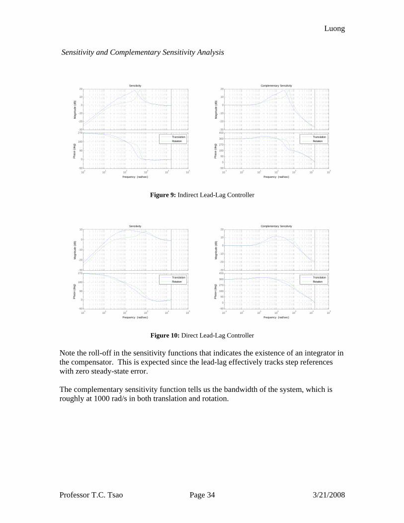
Figure 9: Indirect Lead-Lag Controller
-30
-20
-10
0
10
Mag
nitu
de (d
B)
100
101
102
103
104
105
-90
0
90
180
270
Phas
e (d
eg)
Sensitivity
Frequency (rad/sec)
TranslationRotation
-30
-20
-10
0
10
20
Mag
nitu
de (d
B)
10-1
100
101
102
103
104
105
-90
0
90
180
270
360
450
Phas
e (d
eg)
Complementary Sensitivity
Frequency (rad/sec)
TranslationRotation
Figure 10: Direct Lead-Lag Controller Note the roll-off in the sensitivity functions that indicates the existence of an integrator in the compensator. This is expected since the lead-lag effectively tracks step references with zero steady-state error. The complementary sensitivity function tells us the bandwidth of the system, which is roughly at 1000 rad/s in both translation and rotation.
Luong
Professor T.C. Tsao Page 35 3/21/2008
Robust Stability Analysis
100
101
102
103
104
-30
-25
-20
-15
-10
-5
0
5
10
15
20m
agni
tude
(dB)
Robust Stability: (Wr*T)translation
rad/sec (rad/sec) 10
010
110
210
310
4
-25
-20
-15
-10
-5
0
5
10
15
mag
nitu
de (d
B)
Robust Stability: (Wr*T)rotation
rad/sec (rad/sec)
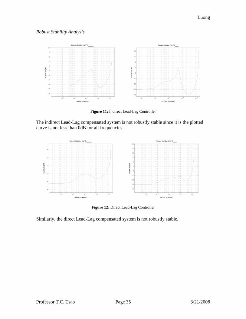
Figure 11: Indirect Lead-Lag Controller
The indirect Lead-Lag compensated system is not robustly stable since it is the plotted curve is not less than 0dB for all frequencies.
100
101
102
103
104
-30
-20
-10
0
10
20
mag
nitu
de (d
B)
Robust Stability: (Wr*T)translation
rad/sec (rad/sec) 10
010
110
210
310
4
-25
-20
-15
-10
-5
0
5
10
15
20
25
mag
nitu
de (d
B)
Robust Stability: (Wr*T)rotation
rad/sec (rad/sec)
Figure 12: Direct Lead-Lag Controller Similarly, the direct Lead-Lag compensated system is not robustly stable.
Luong
Professor T.C. Tsao Page 36 3/21/2008
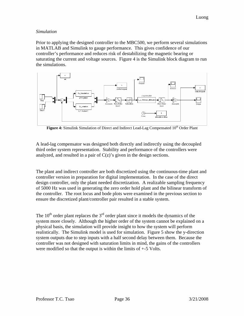
Simulation Prior to applying the designed controller to the MBC500, we perform several simulations in MATLAB and Simulink to gauge performance. This gives confidence of our controller’s performance and reduces risk of destabilizing the magnetic bearing or saturating the current and voltage sources. Figure 4 is the Simulink block diagram to run the simulations.
Figure 4: Simulink Simulation of Direct and Indirect Lead-Lag Compensated 10th Order Plant
A lead-lag compensator was designed both directly and indirectly using the decoupled third order system representation. Stability and performance of the controllers were analyzed, and resulted in a pair of C(z)’s given in the design sections. The plant and indirect controller are both discretized using the continuous-time plant and controller version in preparation for digital implementation. In the case of the direct design controller, only the plant needed discretization. A realizable sampling frequency of 5000 Hz was used in generating the zero order hold plant and the bilinear transform of the controller. The root locus and bode plots were examined in the previous section to ensure the discretized plant/controller pair resulted in a stable system. The 10th order plant replaces the 3rd order plant since it models the dynamics of the system more closely. Although the higher order of the system cannot be explained on a physical basis, the simulation will provide insight to how the system will perform realistically. The Simulink model is used for simulation. Figure 5 show the y-direction system outputs due to step inputs with a half second delay between them. Because the controller was not designed with saturation limits in mind, the gains of the controllers were modified so that the output is within the limits of +-5 Volts.
Luong
Professor T.C. Tsao Page 37 3/21/2008
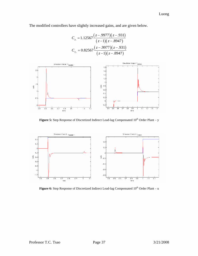
The modified controllers have slightly increased gains, and are given below.
( )( )( )( )( )( )( )( )
1
2
.9977 .9311.12567
1 .8947
.9977 .9310.82567
1 .8947
y
y
z zC
z z
z zC
z z
− −=
− −
− −=
− −
Figure 5: Step Response of Discretized Indirect Lead-lag Compensated 10th Order Plant – y
Figure 6: Step Response of Discretized Indirect Lead-lag Compensated 10th Order Plant – u
Luong
Professor T.C. Tsao Page 38 3/21/2008
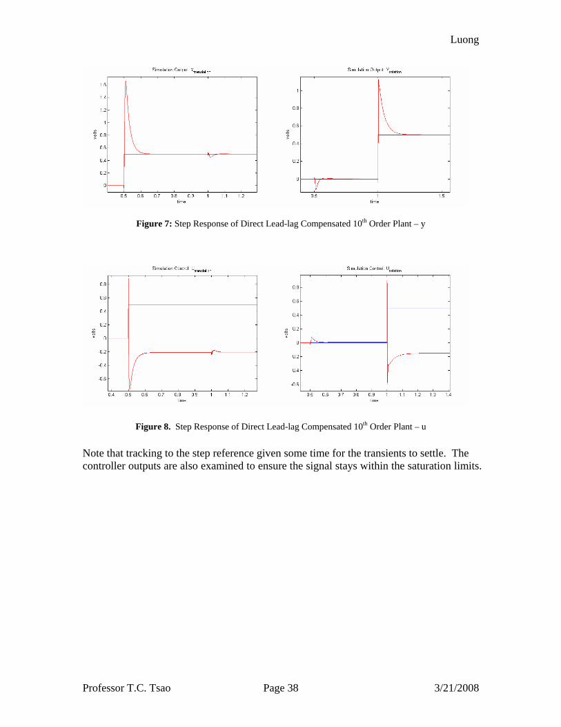
Figure 7: Step Response of Direct Lead-lag Compensated 10th Order Plant – y
Figure 8. Step Response of Direct Lead-lag Compensated 10th Order Plant – u Note that tracking to the step reference given some time for the transients to settle. The controller outputs are also examined to ensure the signal stays within the saturation limits.
Luong
Professor T.C. Tsao Page 39 3/21/2008
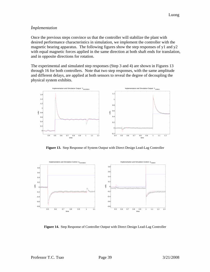
Implementation Once the previous steps convince us that the controller will stabilize the plant with desired performance characteristics in simulation, we implement the controller with the magnetic bearing apparatus. The following figures show the step responses of y1 and y2 with equal magnetic forces applied in the same direction at both shaft ends for translation, and in opposite directions for rotation. The experimental and simulated step responses (Step 3 and 4) are shown in Figures 13 through 16 for both controllers. Note that two step responses, with the same amplitude and different delays, are applied at both sensors to reveal the degree of decoupling the physical system exhibits.
0.4 0.5 0.6 0.7 0.8 0.9 1 1.1 1.2
0
0.2
0.4
0.6
0.8
1
1.2
1.4
1.6
Implementation and Simulation Output: Ytranslation
time
volts
0.4 0.5 0.6 0.7 0.8 0.9 1 1.1 1.2-0.2
0
0.2
0.4
0.6
0.8
1
1.2
Implementation and Simulation Output: Yrotation
time
volts
Figure 13. Step Response of System Output with Direct Design Lead-Lag Controller
0.5 0.6 0.7 0.8 0.9 1 1.1
-0.8
-0.6
-0.4
-0.2
0
0.2
0.4
0.6
0.8
Implementation and Simulation Control: Utranslation
time
volts
0.5 0.6 0.7 0.8 0.9 1 1.1 1.2 1.3
-0.8
-0.6
-0.4
-0.2
0
0.2
0.4
0.6
0.8
Implementation and Simulation Control: Urotation
time
volts
Figure 14. Step Response of Controller Output with Direct Design Lead-Lag Controller
Luong
Professor T.C. Tsao Page 40 3/21/2008
0.4 0.5 0.6 0.7 0.8 0.9 1 1.1 1.2
0
0.5
1
1.5
2
2.5
Implementation and Simulation Output: Ytranslation
time
volts
0.4 0.5 0.6 0.7 0.8 0.9 1 1.1 1.2
-0.2
0
0.2
0.4
0.6
0.8
1
1.2
1.4
1.6
1.8
Implementation and Simulation Output: Yrotation
time
volts
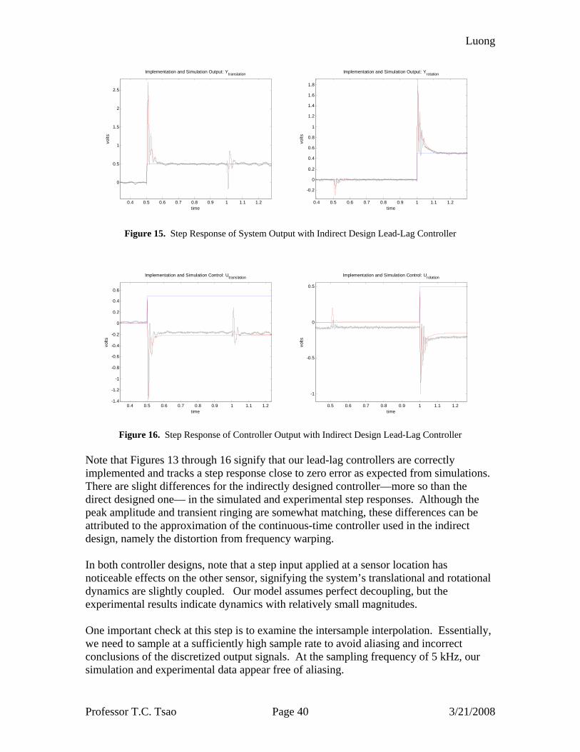
Figure 15. Step Response of System Output with Indirect Design Lead-Lag Controller
0.4 0.5 0.6 0.7 0.8 0.9 1 1.1 1.2-1.4
-1.2
-1
-0.8
-0.6
-0.4
-0.2
0
0.2
0.4
0.6
Implementation and Simulation Control: Utranslation
time
volts
0.5 0.6 0.7 0.8 0.9 1 1.1 1.2
-1
-0.5
0
0.5
Implementation and Simulation Control: Urotation
time
volts
Figure 16. Step Response of Controller Output with Indirect Design Lead-Lag Controller Note that Figures 13 through 16 signify that our lead-lag controllers are correctly implemented and tracks a step response close to zero error as expected from simulations. There are slight differences for the indirectly designed controller—more so than the direct designed one— in the simulated and experimental step responses. Although the peak amplitude and transient ringing are somewhat matching, these differences can be attributed to the approximation of the continuous-time controller used in the indirect design, namely the distortion from frequency warping. In both controller designs, note that a step input applied at a sensor location has noticeable effects on the other sensor, signifying the system’s translational and rotational dynamics are slightly coupled. Our model assumes perfect decoupling, but the experimental results indicate dynamics with relatively small magnitudes. One important check at this step is to examine the intersample interpolation. Essentially, we need to sample at a sufficiently high sample rate to avoid aliasing and incorrect conclusions of the discretized output signals. At the sampling frequency of 5 kHz, our simulation and experimental data appear free of aliasing.
Luong
Professor T.C. Tsao Page 41 3/21/2008
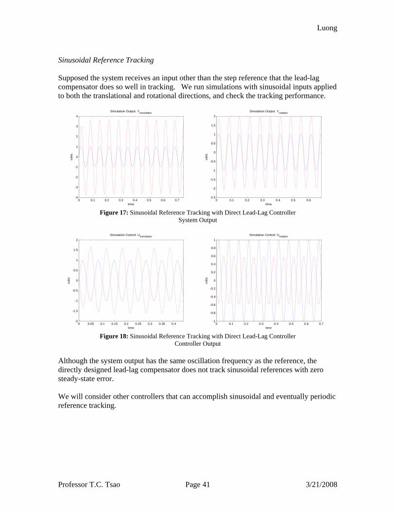
Sinusoidal Reference Tracking Supposed the system receives an input other than the step reference that the lead-lag compensator does so well in tracking. We run simulations with sinusoidal inputs applied to both the translational and rotational directions, and check the tracking performance.
0 0.1 0.2 0.3 0.4 0.5 0.6 0.7-4
-3
-2
-1
0
1
2
3
4Simulation Output: Ytranslation
time
volts
0 0.1 0.2 0.3 0.4 0.5 0.6
-2.5
-2
-1.5
-1
-0.5
0
0.5
1
1.5
2Simulation Output: Yrotation
timevo
lts
Figure 17: Sinusoidal Reference Tracking with Direct Lead-Lag Controller System Output
0 0.05 0.1 0.15 0.2 0.25 0.3 0.35 0.4-2
-1.5
-1
-0.5
0
0.5
1
1.5
2Simulation Control: Utranslation
time
volts
0 0.1 0.2 0.3 0.4 0.5 0.6 0.7
-1
-0.8
-0.6
-0.4
-0.2
0
0.2
0.4
0.6
0.8
1Simulation Control: Urotation
time
volts
Figure 18: Sinusoidal Reference Tracking with Direct Lead-Lag Controller
Controller Output
Although the system output has the same oscillation frequency as the reference, the directly designed lead-lag compensator does not track sinusoidal references with zero steady-state error. We will consider other controllers that can accomplish sinusoidal and eventually periodic reference tracking.

Luong
Professor T.C. Tsao Page 42 3/21/2008
STATE OBSERVER FEEDBACK CONTROLLER This controller leverages modern control design techniques, in other words, state-space form. The graphical representation that classical design features is not apparent in modern design. However, designers have a richer mathematical framework for placing closed-loop system poles by designing a feedback gain for achieving that. Often times, state variables are not available for control design. Estimation techniques are thus needed. The Luenberger Observer is explored and trialed in constructing a state feedback controller for the MBC500. Formulation A controller for the system (A,B) can be designed using state feedback if and only if (A,B) is controllable. The locations of the system’s closed-loop poles can be placed anywhere with the appropriate state feedback gain K. We can represent the system in the state-space form
( 1) ( ) ( )( ) ( )
x k Ax k Bu ky k Cx k
+ = +=
with the state feedback and feed-forward control law
( ) ( ) ( )u k Kx k Nr k= − + With the control law, the closed-loop system is
( 1) ( ) ( ) ( )( ) ( )
x k A BK x k BNu ky k Cx k
+ = − +=
The associated transfer function is
[ ] 1( ) ( ) ( )Y z C zI A BK BNr z−= − −
To examine the phase and gain margins of the system, we look at the characteristic equation
11 ( ) ( ) 0K zI A Bu z−+ − =
where the loop gain is
1( ) ( )L z K zI A B−= −
Luong
Professor T.C. Tsao Page 43 3/21/2008
The gain K can be chosen to have the specified closed-loop poles using MATLAB’s place command with the matrices (A,B), and vector P containing the desired poles. State feedback relies on the fact that information of the states is available. In practice, this is often not the case. We can augment the state feedback controller with state estimation. The closed-loop Luenberger observer includes extensive information of the states from output measurements. In this scheme, we examine the error dynamics defined as
ˆ( ) ( ) ( )x k x k x k= − We desire the error dynamics to converge to 0 in the steady-state so that our estimated states are close to the actual ones. The observer state-space equation is
( 1) ( ) ( )( ) ( )
x k Ax k LCx kA LC x k
+ = −= −
The observer gain L is usually chosen to place the closed-loop poles such that the state estimation is quicker than the state feedback. The observer poles can be placed at any location if and only if (A,C) is observable. MATLAB’S place(A’,C’,P) command is often used for pole placement. The state estimation feedback can be written as the following:
[ ]
( 1) ( )( )
( 1) 0 ( ) 0
( )( ) 0
( )
x k A BK BK x k BN r t
x k A LC x k
x ky k C
x k
+ − −⎡ ⎤ ⎡ ⎤ ⎡ ⎤ ⎡ ⎤= + ⋅⎢ ⎥ ⎢ ⎥ ⎢ ⎥ ⎢ ⎥+ −⎣ ⎦ ⎣ ⎦ ⎣ ⎦ ⎣ ⎦
⎡ ⎤= ⎢ ⎥
⎣ ⎦
The closed-loop characteristic equation of the system above is given by
[ ] [ ]( )det det ( ) det ( )
0 ( )zI A BK BK
zI A BK zI A LCzI A LC
− −⎡ ⎤= − − ⋅ − −⎢ ⎥− −⎣ ⎦
This shows that n of the closed-loop eigenvalues, or poles, are from the state feedback design and the other n eigenvalues are from the observer compensator design. This highlights the separation principle i.e. the state feedback control poles can be designed separately from the observer poles. To examine the phase and gain margins of the modified system, we look at the characteristic equation
[ ] 1 11 ( ) ( ) 0K zI A LC BK LC zI A B− −+ − − − − =
Luong
Professor T.C. Tsao Page 44 3/21/2008
where the modified loop gain is
[ ] 1 1( ) ( ) ( )L z K zI A LC BK LC zI A B− −= − − − − Internal Model Augmentation
For reference tracking with zero steady-state error, we can include a form of the reference signal into the controller. This is called Internal Model Control. For step reference tracking, we can build integral control into this controller through a state augmentation. We accomplish this by augmenting the model of the plant with an integrator, which adds an error integral output to the existing plant output. We define the error signal as
( ) ( ) ( ) ( ) ( )( )ˆ ˆe k y k y k C x k x k= − = − The propagated integral of the error is formulated as
( ) [ ] [ ]1 ( ) ( ) ( ) ( ) ( ) ( )e k e k y k r k e k Cx k r k+ = + − = + − The augmented state equation is then
( 1) 0 ( ) 0( ) ( )
( 1) 1 ( ) 0 1
( )' ' ( ) ' ( )
( )
x k A x k Bu k r k
e k C e k
x kA B u k N r k
e k
+⎡ ⎤ ⎡ ⎤ ⎡ ⎤ ⎡ ⎤ ⎡ ⎤= + +⎢ ⎥ ⎢ ⎥ ⎢ ⎥ ⎢ ⎥ ⎢ ⎥+ −⎣ ⎦ ⎣ ⎦ ⎣ ⎦ ⎣ ⎦ ⎣ ⎦
⎡ ⎤= + +⎢ ⎥
⎣ ⎦
The modified control gain has the following form
[ ]|s iK K K=
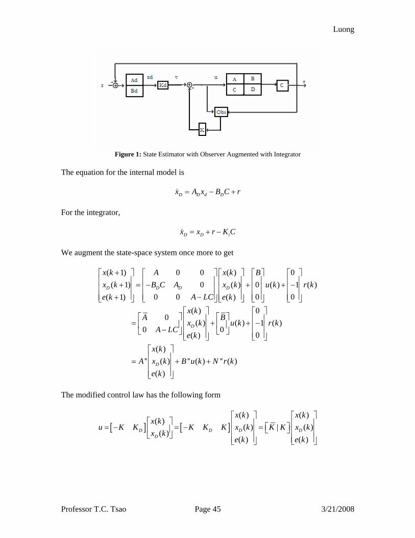
where iK is the added element is the gain for the integrator. As before, the place command with the new 'A and 'B matrices can be used to determine the feedback gain. The block diagram of this state-space system is shown in Figure 1.
Luong
Professor T.C. Tsao Page 45 3/21/2008
Figure 1: State Estimator with Observer Augmented with Integrator
The equation for the internal model is
D D d Dx A x B C r= − +
For the integrator,
D D ix x r K C= + − We augment the state-space system once more to get
( 1) 0 0 ( ) 0( 1) 0 ( ) 0 ( ) 1 ( )
0 0 0 0( 1) ( )
( ) 00
( ) ( ) 1 ( )00
0( )
( )'' ( )
(
D D D D
D
D
x k A x k Bx k B C A x k u k r k
A LCe k e k
x kBA
x k u k r kA LC
e k
x kA x k
e
+⎡ ⎤ ⎡ ⎤ ⎡ ⎤ ⎡ ⎤ ⎡ ⎤⎢ ⎥ ⎢ ⎥ ⎢ ⎥ ⎢ ⎥ ⎢ ⎥+ = − + + −⎢ ⎥ ⎢ ⎥ ⎢ ⎥ ⎢ ⎥ ⎢ ⎥⎢ ⎥ ⎢ ⎥ ⎢ ⎥ ⎢ ⎥ ⎢ ⎥−+⎣ ⎦ ⎣ ⎦ ⎣ ⎦ ⎣ ⎦ ⎣ ⎦
⎡ ⎤ ⎡ ⎤⎡ ⎤ ⎡ ⎤⎢ ⎥ ⎢ ⎥= + + −⎢ ⎥ ⎢ ⎥⎢ ⎥ ⎢ ⎥− ⎣ ⎦⎣ ⎦ ⎢ ⎥ ⎢ ⎥⎣ ⎦ ⎣ ⎦
= '' ( ) '' ( ))
B u k N r kk
⎡ ⎤⎢ ⎥ + +⎢ ⎥⎢ ⎥⎣ ⎦
The modified control law has the following form
[ ] [ ]( ) ( )
( )( ) | ( )
( )( ) ( )
D D D DD
x k x kx k
u K K K K K x k K K x kx k
e k e k
⎡ ⎤ ⎡ ⎤⎡ ⎤ ⎢ ⎥ ⎢ ⎥⎡ ⎤= − = − =⎢ ⎥ ⎣ ⎦⎢ ⎥ ⎢ ⎥⎣ ⎦ ⎢ ⎥ ⎢ ⎥⎣ ⎦ ⎣ ⎦
Luong
Professor T.C. Tsao Page 46 3/21/2008
The closed loop “A” matrix is A BK− :
0" "
00
0
BAA B K K K
A LC
A BK BKA LC
⎡ ⎤ ⎡ ⎤⎡ ⎤− = −⎢ ⎥ ⎢ ⎥ ⎣ ⎦− ⎣ ⎦⎣ ⎦
⎡ ⎤−= ⎢ ⎥−⎣ ⎦
We arrive at an upper triangular A-matrix once again, so the separation principle also applies in determining feedback and observer gains. For robust stability analysis, we need to calculate the sensitivity and complementary sensitivity functions. The loop gain from the integrator output v to y is
( )( ) 1
11( ) ( )
11I
IKL z G z K zI A LC L
zK zI A LC B−
−⎛ ⎞= ⋅ ⋅ − + +⎜ ⎟−⎝ ⎠+ − +
The derivation is provided in the Appendix. The sensitivity and complementary sensitivity functions for the integrator system are
( )
( ) ( )
( )
( ) ( )
1
1 1
1
1 1
111 ( ) 1 ( )
1
( )11
1 ( )1
I
I
I
K zI A LC BS
KL z K zI A LC B G z K zI A LC Lz
KG z K zI A LC LzT S
KK zI A LC B G z K zI A LC Lz
−
− −
−
− −
+ − += =
+ ⎛ ⎞+ − + + ⋅ − + +⎜ ⎟−⎝ ⎠⎛ ⎞⋅ − + +⎜ ⎟−⎝ ⎠= − =
⎛ ⎞+ − + + ⋅ − + +⎜ ⎟−⎝ ⎠
The T is also used in robust stability analysis. The characteristic equation of this system is now
( )
( )( ) 1
1
1 0
11 ( ) 011
i
I
L z
KG z K zI A LC LzK zI A LC B
−
−
+ =
⎛ ⎞+ ⋅ ⋅ − + + =⎜ ⎟−⎝ ⎠+ − +
Luong
Professor T.C. Tsao Page 47 3/21/2008
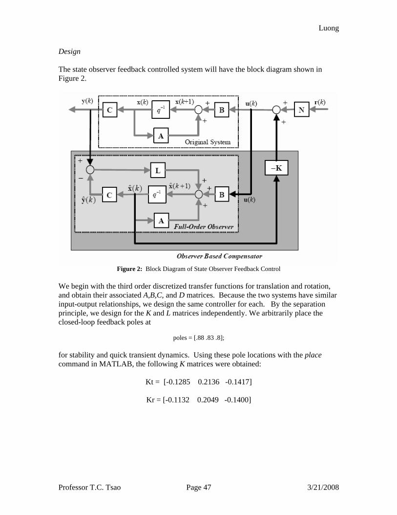
Design The state observer feedback controlled system will have the block diagram shown in Figure 2.
Figure 2: Block Diagram of State Observer Feedback Control
We begin with the third order discretized transfer functions for translation and rotation, and obtain their associated A,B,C, and D matrices. Because the two systems have similar input-output relationships, we design the same controller for each. By the separation principle, we design for the K and L matrices independently. We arbitrarily place the closed-loop feedback poles at
poles = [.88 .83 .8];
for stability and quick transient dynamics. Using these pole locations with the place command in MATLAB, the following K matrices were obtained:
Kt = [-0.1285 0.2136 -0.1417]
Kr = [-0.1132 0.2049 -0.1400]
Luong
Professor T.C. Tsao Page 48 3/21/2008
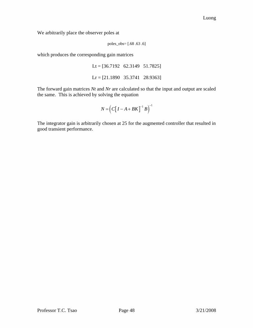
We arbitrarily place the observer poles at
poles_obs= [.68 .63 .6]
which produces the corresponding gain matrices
Lt = [36.7192 62.3149 51.7825]
Lr = [21.1890 35.3741 28.9363]
The forward gain matrices Nt and Nr are calculated so that the input and output are scaled the same. This is achieved by solving the equation
[ ]( ) 11N C I A BK B−−= − +
The integrator gain is arbitrarily chosen at 25 for the augmented controller that resulted in good transient performance.
Luong
Professor T.C. Tsao Page 49 3/21/2008
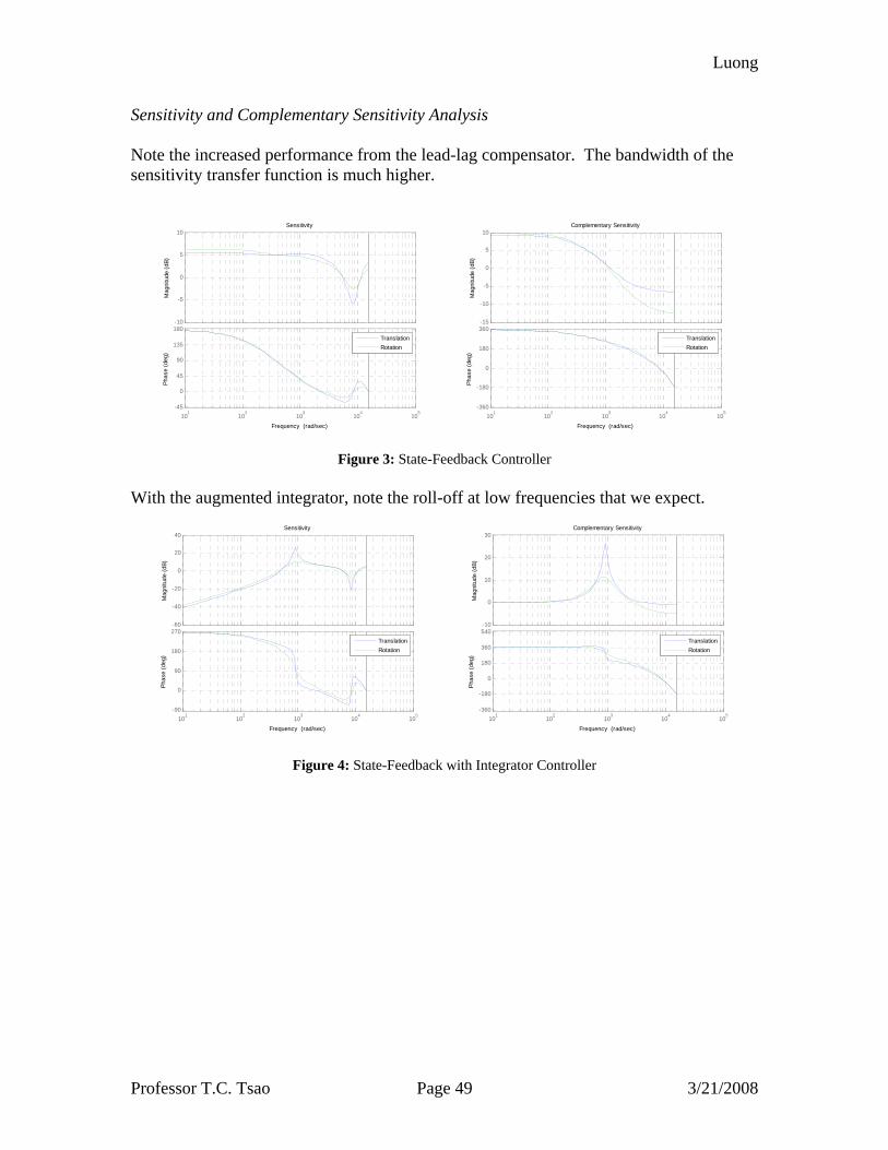
Sensitivity and Complementary Sensitivity Analysis Note the increased performance from the lead-lag compensator. The bandwidth of the sensitivity transfer function is much higher.
-10
-5
0
5
10
Mag
nitu
de (d
B)
101
102
103
104
105
-45
0
45
90
135
180
Phas
e (d
eg)
Sensitivity
Frequency (rad/sec)
TranslationRotation
-15
-10
-5
0
5
10
Mag
nitu
de (d
B)
101
102
103
104
105
-360
-180
0
180
360
Phas
e (d
eg)
Complementary Sensitivity
Frequency (rad/sec)
TranslationRotation
Figure 3: State-Feedback Controller
With the augmented integrator, note the roll-off at low frequencies that we expect.
-60
-40
-20
0
20
40
Mag
nitu
de (d
B)
101
102
103
104
105
-90
0
90
180
270
Phas
e (d
eg)
Sensitivity
Frequency (rad/sec)
TranslationRotation
-10
0
10
20
30
Mag
nitu
de (d
B)
101
102
103
104
105
-360
-180
0
180
360
540
Phas
e (d
eg)
Complementary Sensitivity
Frequency (rad/sec)
TranslationRotation
Figure 4: State-Feedback with Integrator Controller

Luong
Professor T.C. Tsao Page 50 3/21/2008
Robust Stability Analysis Note that the state-feedback controller, as designed, is not robustly stable in either direction.
101
102
103
104
-20
-10
0
10
20
30
40
mag
nitu
de (d
B)
Robust Stability: (Wr*T)translation
rad/sec (rad/sec)10
110
210
310
4
-20
-10
0
10
20
30
mag
nitu
de (d
B)
Robust Stability: (Wr*T)rotation
rad/sec (rad/sec)
Figure 5: State-Feedback Controller
101
102
103
104
-30
-20
-10
0
10
20
30
40
50
mag
nitu
de (d
B)
Robust Stability: (Wr*T)translation
rad/sec (rad/sec) 10
110
210
310
4
-20
-10
0
10
20
30
40
mag
nitu
de (d
B)
Robust Stability: (Wr*T)rotation
rad/sec (rad/sec)
Figure 6: State-Feedback with Integrator Controller
Luong
Professor T.C. Tsao Page 51 3/21/2008
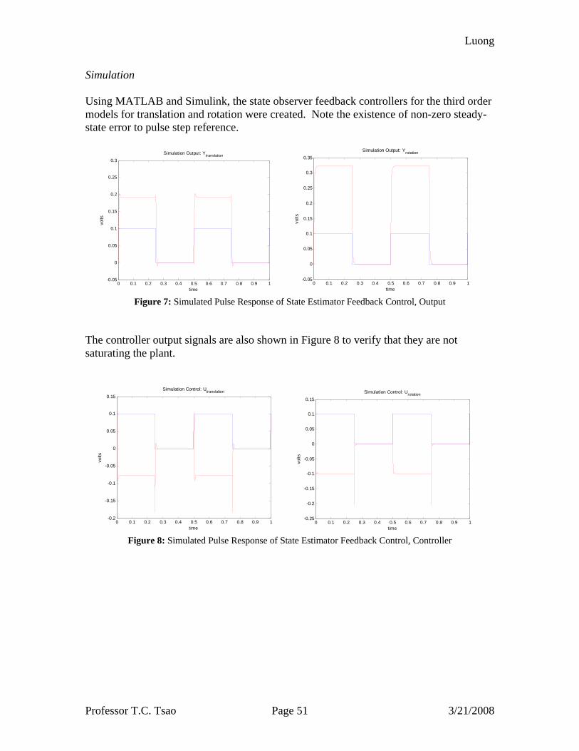
Simulation Using MATLAB and Simulink, the state observer feedback controllers for the third order models for translation and rotation were created. Note the existence of non-zero steady-state error to pulse step reference.
0 0.1 0.2 0.3 0.4 0.5 0.6 0.7 0.8 0.9 1-0.05
0
0.05
0.1
0.15
0.2
0.25
0.3Simulation Output: Ytranslation
time
volts
0 0.1 0.2 0.3 0.4 0.5 0.6 0.7 0.8 0.9 1-0.05
0
0.05
0.1
0.15
0.2
0.25
0.3
0.35Simulation Output: Yrotation
timevo
lts
Figure 7: Simulated Pulse Response of State Estimator Feedback Control, Output
The controller output signals are also shown in Figure 8 to verify that they are not saturating the plant.
0 0.1 0.2 0.3 0.4 0.5 0.6 0.7 0.8 0.9 1-0.2
-0.15
-0.1
-0.05
0
0.05
0.1
0.15Simulation Control: Utranslation
time
volts
0 0.1 0.2 0.3 0.4 0.5 0.6 0.7 0.8 0.9 1-0.25
-0.2
-0.15
-0.1
-0.05
0
0.05
0.1
0.15Simulation Control: Urotation
time
volts
Figure 8: Simulated Pulse Response of State Estimator Feedback Control, Controller
Luong
Professor T.C. Tsao Page 52 3/21/2008
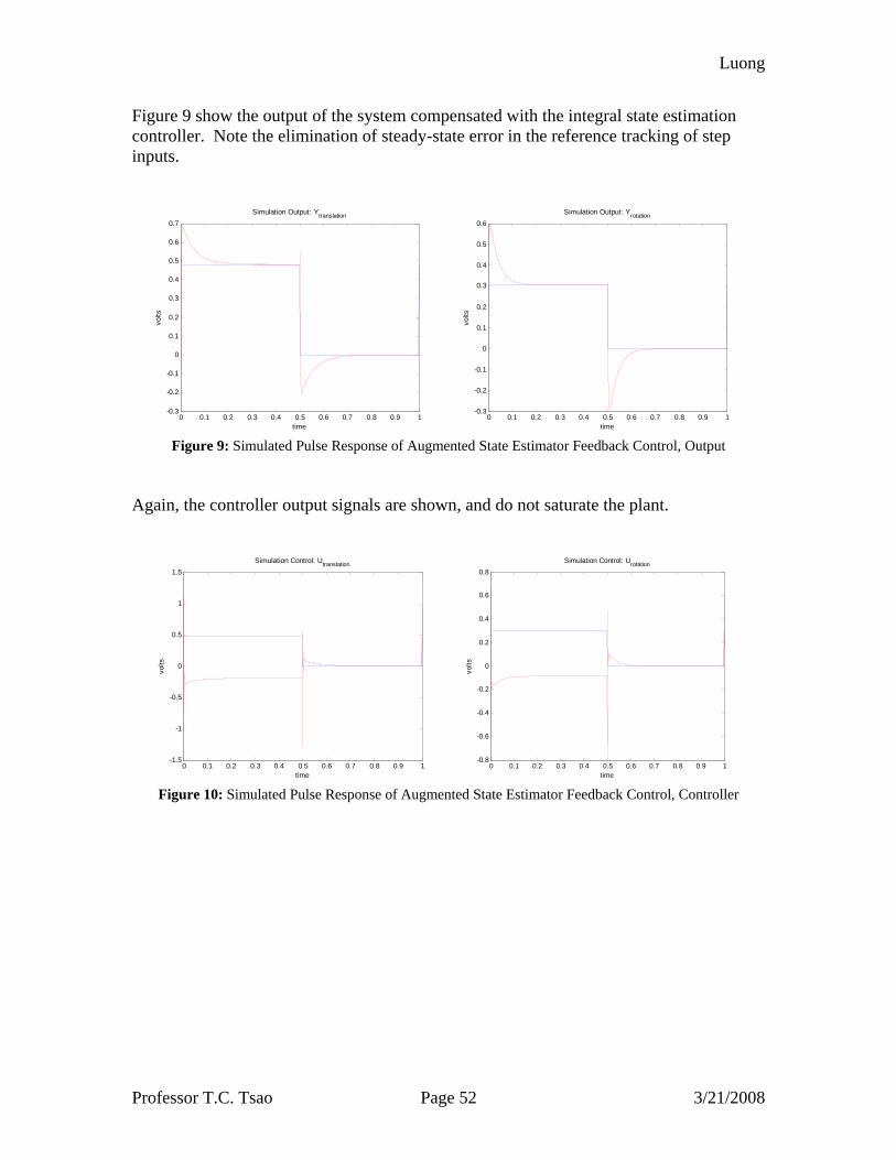
Figure 9 show the output of the system compensated with the integral state estimation controller. Note the elimination of steady-state error in the reference tracking of step inputs.
0 0.1 0.2 0.3 0.4 0.5 0.6 0.7 0.8 0.9 1-0.3
-0.2
-0.1
0
0.1
0.2
0.3
0.4
0.5
0.6
0.7Simulation Output: Ytranslation
time
volts
0 0.1 0.2 0.3 0.4 0.5 0.6 0.7 0.8 0.9 1-0.3
-0.2
-0.1
0
0.1
0.2
0.3
0.4
0.5
0.6Simulation Output: Yrotation
time
volts
Figure 9: Simulated Pulse Response of Augmented State Estimator Feedback Control, Output
Again, the controller output signals are shown, and do not saturate the plant.
0 0.1 0.2 0.3 0.4 0.5 0.6 0.7 0.8 0.9 1-1.5
-1
-0.5
0
0.5
1
1.5Simulation Control: Utranslation
time
volts
0 0.1 0.2 0.3 0.4 0.5 0.6 0.7 0.8 0.9 1-0.8
-0.6
-0.4
-0.2
0
0.2
0.4
0.6
0.8Simulation Control: Urotation
time
volts
Figure 10: Simulated Pulse Response of Augmented State Estimator Feedback Control, Controller
Luong
Professor T.C. Tsao Page 53 3/21/2008
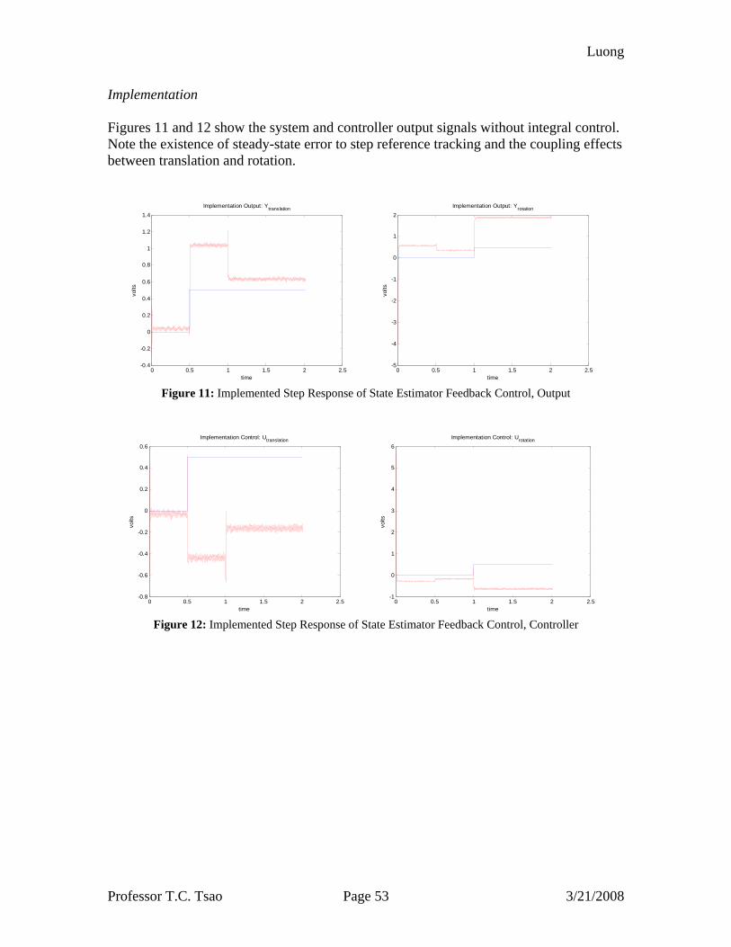
Implementation Figures 11 and 12 show the system and controller output signals without integral control. Note the existence of steady-state error to step reference tracking and the coupling effects between translation and rotation.
0 0.5 1 1.5 2 2.5-0.4
-0.2
0
0.2
0.4
0.6
0.8
1
1.2
1.4Implementation Output: Ytranslation
time
volts
0 0.5 1 1.5 2 2.5-5
-4
-3
-2
-1
0
1
2Implementation Output: Yrotation
timevo
lts
Figure 11: Implemented Step Response of State Estimator Feedback Control, Output
0 0.5 1 1.5 2 2.5-0.8
-0.6
-0.4
-0.2
0
0.2
0.4
0.6Implementation Control: Utranslation
time
volts
0 0.5 1 1.5 2 2.5-1
0
1
2
3
4
5
6Implementation Control: Urotation
time
volts
Figure 12: Implemented Step Response of State Estimator Feedback Control, Controller
Luong
Professor T.C. Tsao Page 54 3/21/2008
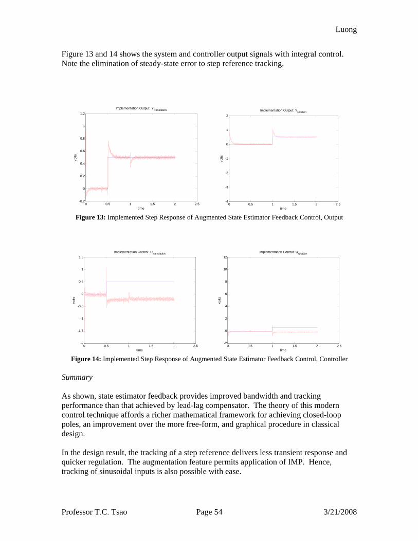
Figure 13 and 14 shows the system and controller output signals with integral control. Note the elimination of steady-state error to step reference tracking.
0 0.5 1 1.5 2 2.5-0.2
0
0.2
0.4
0.6
0.8
1
1.2Implementation Output: Ytranslation
time
volts
0 0.5 1 1.5 2 2.5-4
-3
-2
-1
0
1
2Implementation Output: Yrotation
time
volts
Figure 13: Implemented Step Response of Augmented State Estimator Feedback Control, Output
0 0.5 1 1.5 2 2.5-2
-1.5
-1
-0.5
0
0.5
1
1.5Implementation Control: Utranslation
time
volts
0 0.5 1 1.5 2 2.5-2
0
2
4
6
8
10
12Implementation Control: Urotation
time
volts
Figure 14: Implemented Step Response of Augmented State Estimator Feedback Control, Controller
Summary As shown, state estimator feedback provides improved bandwidth and tracking performance than that achieved by lead-lag compensator. The theory of this modern control technique affords a richer mathematical framework for achieving closed-loop poles, an improvement over the more free-form, and graphical procedure in classical design. In the design result, the tracking of a step reference delivers less transient response and quicker regulation. The augmentation feature permits application of IMP. Hence, tracking of sinusoidal inputs is also possible with ease.
Luong
Professor T.C. Tsao Page 55 3/21/2008
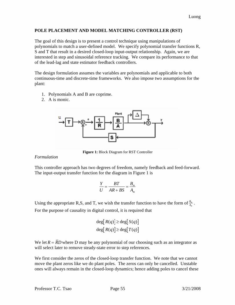
POLE PLACEMENT AND MODEL MATCHING CONTROLLER (RST) The goal of this design is to present a control technique using manipulations of polynomials to match a user-defined model. We specify polynomial transfer functions R, S and T that result in a desired closed-loop input-output relationship. Again, we are interested in step and sinusoidal reference tracking. We compare its performance to that of the lead-lag and state estimator feedback controllers. The design formulation assumes the variables are polynomials and applicable to both continuous-time and discrete-time frameworks. We also impose two assumptions for the plant:
1. Polynomials A and B are coprime. 2. A is monic.
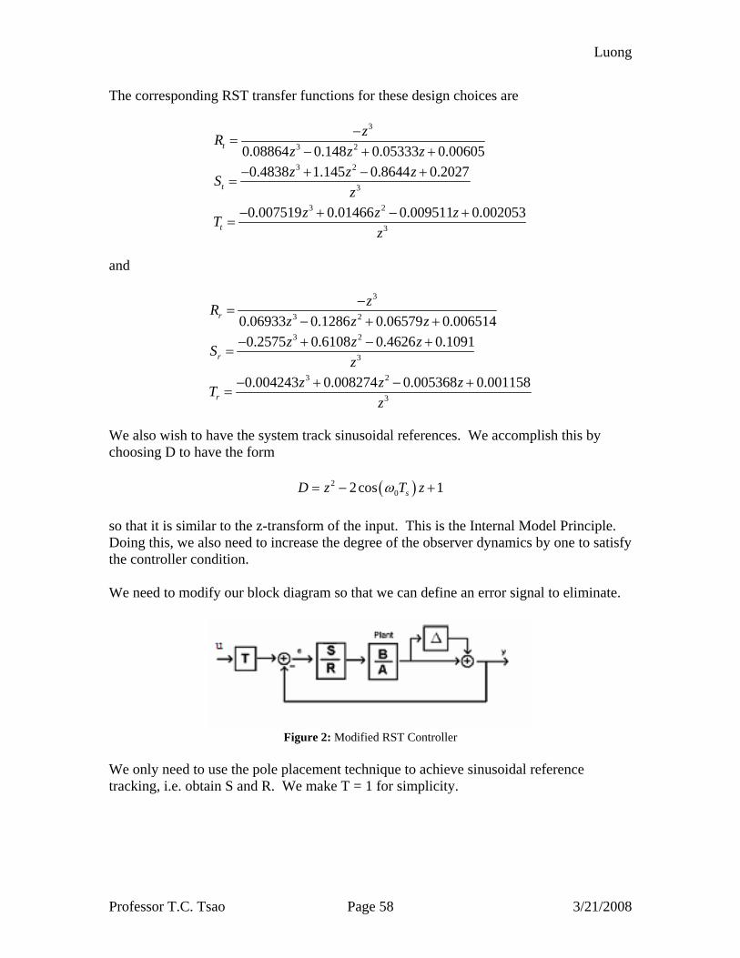
Figure 1: Block Diagram for RST Controller
Formulation This controller approach has two degrees of freedom, namely feedback and feed-forward. The input-output transfer function for the diagram in Figure 1 is
m
m
BY BTU AR BS A
= =+
Using the appropriate R,S, and T, we wish the transfer function to have the form of m
m
BA .
For the purpose of causality in digital control, it is required that
[ ] [ ][ ] [ ]
deg ( ) deg ( )
deg ( ) deg ( )
R q S q
R q T q
≥
≥
We let R RD= where D may be any polynomial of our choosing such as an integrator as will select later to remove steady-state error to step references. We first consider the zeros of the closed-loop transfer function. We note that we cannot move the plant zeros like we do plant poles. The zeros can only be cancelled. Unstable ones will always remain in the closed-loop dynamics; hence adding poles to cancel these
Luong
Professor T.C. Tsao Page 56 3/21/2008
will result in them being unstable. Thus, we separate the unstable and stable zeros by defining
( ) ( ) ( )B q B q B q+ −=
where B+ contains the stable zeros and is monic, and B− contains the unstable zeros of B. The transfer function now has the form
( )( )
m o
m o
Y B B TU ARDB B B S
B B TB ARD B S
B B A BA A B
+ −
+ + −
+ −
+ −
− +
+
=+
=+
= ⋅
where oA represents the cancelled observer dynamics. We note that our polynomials we seek are
m o
R RDBT B A
+=
=
Comparing denominator polynomials, we get the Diophantine Equation
m oARD B S A A−+ = We can solve this equation using the Sylvester Matrix for R and S . The closed-loop poles are
m oA A B+
The designer has freedom to define mA and place the closed-loop poles wherever desired. In this design, we must ensure the following conditions are true for system causality:
[ ] [ ] [ ][ ] [ ] [ ] [ ][ ] [ ] [ ] [ ]
deg deg deg 1
deg 2deg deg deg deg 1
deg deg deg dego m
m m
S A D
A A A B D
A B A B
+
= + −
⎡ ⎤= − − + −⎣ ⎦− ≥ −
Luong
Professor T.C. Tsao Page 57 3/21/2008
For stability margin analysis, we define the sensitivity and complementary sensitivity functions
1
reg
reg
BTTAR BS
BTSAR BS
=+−
=+
For robustness analysis, we define the robust sensitivity function
rBST
AR BS=
+
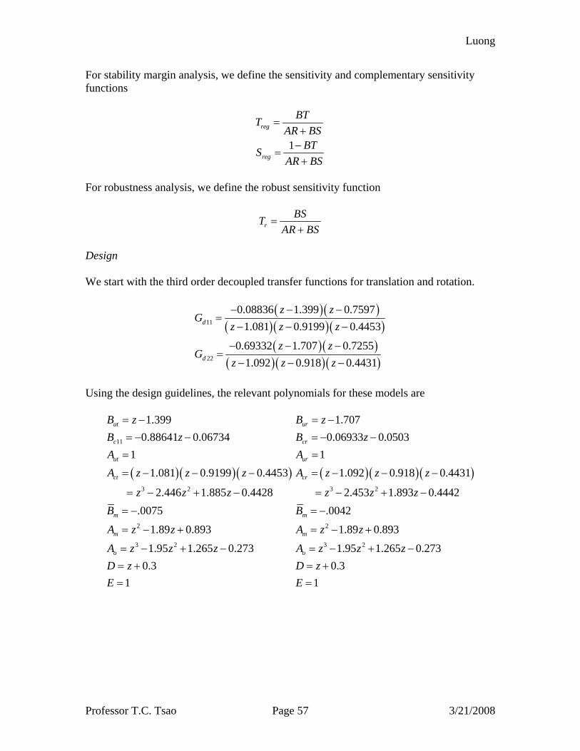
Design We start with the third order decoupled transfer functions for translation and rotation.
( )( )( )( )( )
( )( )( )( )( )
11
22
0.08836 1.399 0.75971.081 0.9199 0.4453
0.69332 1.707 0.72551.092 0.918 0.4431
d
d
z zG
z z z
z zG
z z z
− − −=
− − −
− − −=
− − −
Using the design guidelines, the relevant polynomials for these models are
( )( )( )
11
3 2
2
3 2
1.3990.88641 0.06734
11.081 0.9199 0.4453
2.446 1.885 0.4428.0075
1.89 0.893
1.95 1.265 0.2730.3
1
ut
c
ut
ct
m
m
o
B zB zAA z z z
z z zB
A z z
A z z zD zE
= −= − −=
= − − −
= − + −
= −
= − +
= − + −= +=
( )( )( )3 2
2
3 2
1.7070.06933 0.0503
11.092 0.918 0.4431
2.453 1.893 0.4442.0042
1.89 0.893
1.95 1.265 0.2730.3
1
ur
cr
ur
cr
m
m
o
B zB zAA z z z
z z zB
A z z
A z z zD zE
= −= − −=
= − − −
= − + −
= −
= − +
= − + −= +=
Luong
Professor T.C. Tsao Page 58 3/21/2008
The corresponding RST transfer functions for these design choices are
3
3 2
3 2
3
3 2
3
0.08864 0.148 0.05333 0.006050.4838 1.145 0.8644 0.2027
0.007519 0.01466 0.009511 0.002053
t
t
t
zRz z zz z zS
zz z zT
z
−=
− + +− + − +
=
− + − +=
and
3
3 2
3 2
3
3 2
3
0.06933 0.1286 0.06579 0.0065140.2575 0.6108 0.4626 0.1091
0.004243 0.008274 0.005368 0.001158
r
r
r
zRz z zz z zS
zz z zT
z
−=
− + +− + − +
=
− + − +=
We also wish to have the system track sinusoidal references. We accomplish this by choosing D to have the form
( )202cos 1sD z T zω= − +
so that it is similar to the z-transform of the input. This is the Internal Model Principle. Doing this, we also need to increase the degree of the observer dynamics by one to satisfy the controller condition. We need to modify our block diagram so that we can define an error signal to eliminate.
Figure 2: Modified RST Controller
We only need to use the pole placement technique to achieve sinusoidal reference tracking, i.e. obtain S and R. We make T = 1 for simplicity.
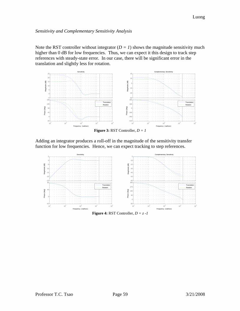
Luong
Professor T.C. Tsao Page 59 3/21/2008
Sensitivity and Complementary Sensitivity Analysis Note the RST controller without integrator (D = 1) shows the magnitude sensitivity much higher than 0 dB for low frequencies. Thus, we can expect it this design to track step references with steady-state error. In our case, there will be significant error in the translation and slightly less for rotation.
-5
0
5
10
15
20
25
Mag
nitu
de (d
B)
101
102
103
104
105
-45
0
45
90
135
180
Phas
e (d
eg)
Sensitivity
Frequency (rad/sec)
TranslationRotation
-60
-40
-20
0
20
40
Mag
nitu
de (d
B)
101
102
103
104
105
-540
-360
-180
0
180
360
Phas
e (d
eg)
Complementary Sensitivity
Frequency (rad/sec)
TranslationRotation
Figure 3: RST Controller, D = 1
Adding an integrator produces a roll-off in the magnitude of the sensitivity transfer function for low frequencies. Hence, we can expect tracking to step references.
-25
-20
-15
-10
-5
0
5
Mag
nitu
de (d
B)
101
102
103
104
105
-45
0
45
90
Phas
e (d
eg)
Sensitivity
Frequency (rad/sec)
TranslationRotation
-60
-50
-40
-30
-20
-10
0
Mag
nitu
de (d
B)
101
102
103
104
105
-90
0
90
180
270
360
Phas
e (d
eg)
Complementary Sensitivity
Frequency (rad/sec)
TranslationRotation
Figure 4: RST Controller, D = z -1
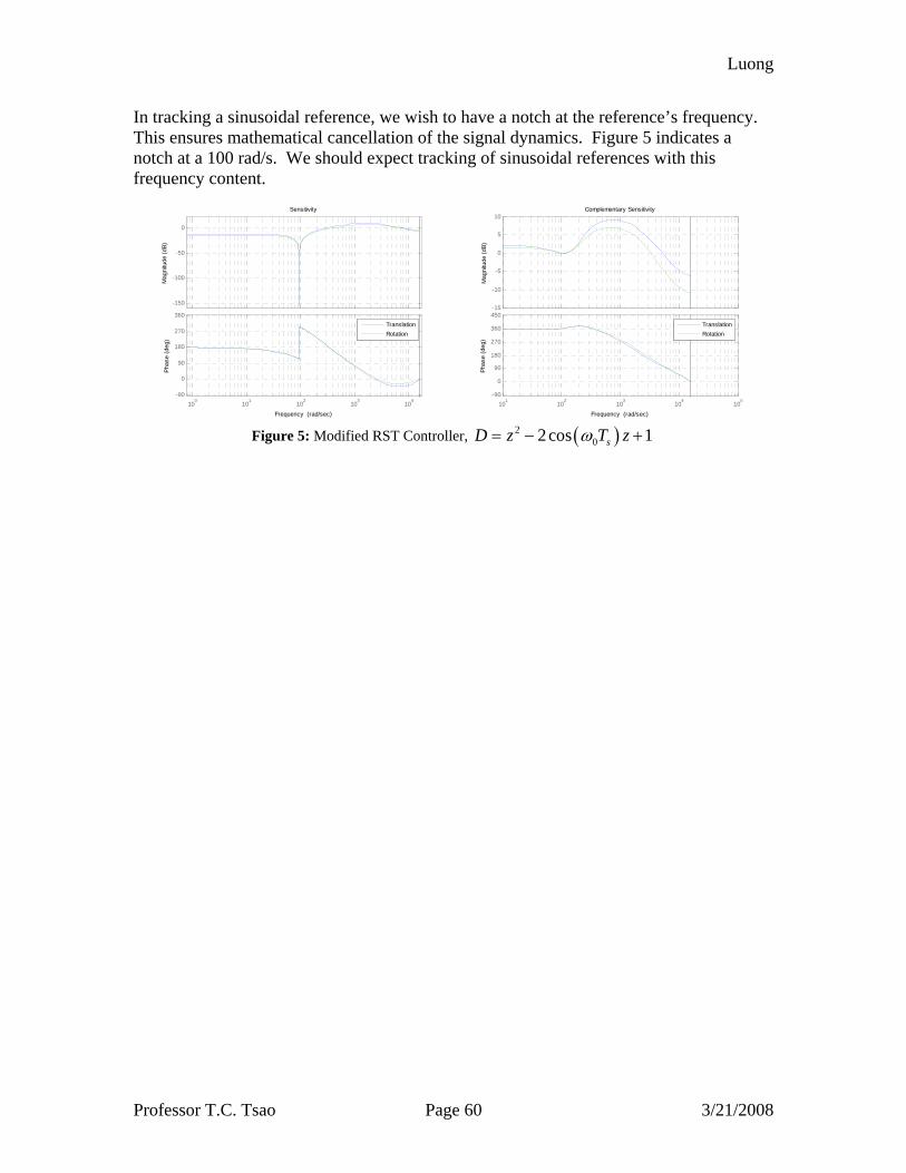
Luong
Professor T.C. Tsao Page 60 3/21/2008
In tracking a sinusoidal reference, we wish to have a notch at the reference’s frequency. This ensures mathematical cancellation of the signal dynamics. Figure 5 indicates a notch at a 100 rad/s. We should expect tracking of sinusoidal references with this frequency content.
-150
-100
-50
0
Mag
nitu
de (d
B)
100
101
102
103
104
-90
0
90
180
270
360
Phas
e (d
eg)
Sensitivity
Frequency (rad/sec)
TranslationRotation
-15
-10
-5
0
5
10
Mag
nitu
de (d
B)
101
102
103
104
105
-90
0
90
180
270
360
450
Phas
e (d
eg)
Complementary Sensitivity
Frequency (rad/sec)
TranslationRotation
Figure 5: Modified RST Controller, ( )2
02cos 1sD z T zω= − +
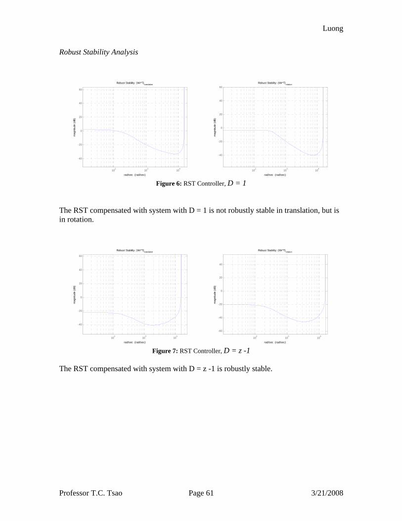
Luong
Professor T.C. Tsao Page 61 3/21/2008
Robust Stability Analysis
102
103
104
-40
-20
0
20
40
60
mag
nitu
de (d
B)
Robust Stability: (Wr*T)translation
rad/sec (rad/sec) 10
210
310
4
-40
-20
0
20
40
60
mag
nitu
de (d
B)
Robust Stability: (Wr*T)rotation
rad/sec (rad/sec) Figure 6: RST Controller, D = 1
The RST compensated with system with D = 1 is not robustly stable in translation, but is in rotation.
102
103
104
-40
-20
0
20
40
60
mag
nitu
de (d
B)
Robust Stability: (Wr*T)translation
rad/sec (rad/sec) 10
210
310
4
-60
-40
-20
0
20
40
mag
nitu
de (d
B)
Robust Stability: (Wr*T)rotation
rad/sec (rad/sec) Figure 7: RST Controller, D = z -1
The RST compensated with system with D = z -1 is robustly stable.
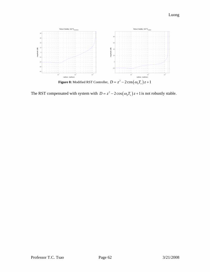
Luong
Professor T.C. Tsao Page 62 3/21/2008
102
103
104
-40
-30
-20
-10
0
10
20
30
40
mag
nitu
de (d
B)
Robust Stability: (Wr*T)translation
rad/sec (rad/sec) 10
210
310
4
-20
0
20
40
60
80
mag
nitu
de (d
B)
Robust Stability: (Wr*T)rotation
rad/sec (rad/sec) Figure 8: Modified RST Controller, ( )2
02cos 1sD z T zω= − +
The RST compensated with system with ( )2
02cos 1sD z T zω= − + is not robustly stable.
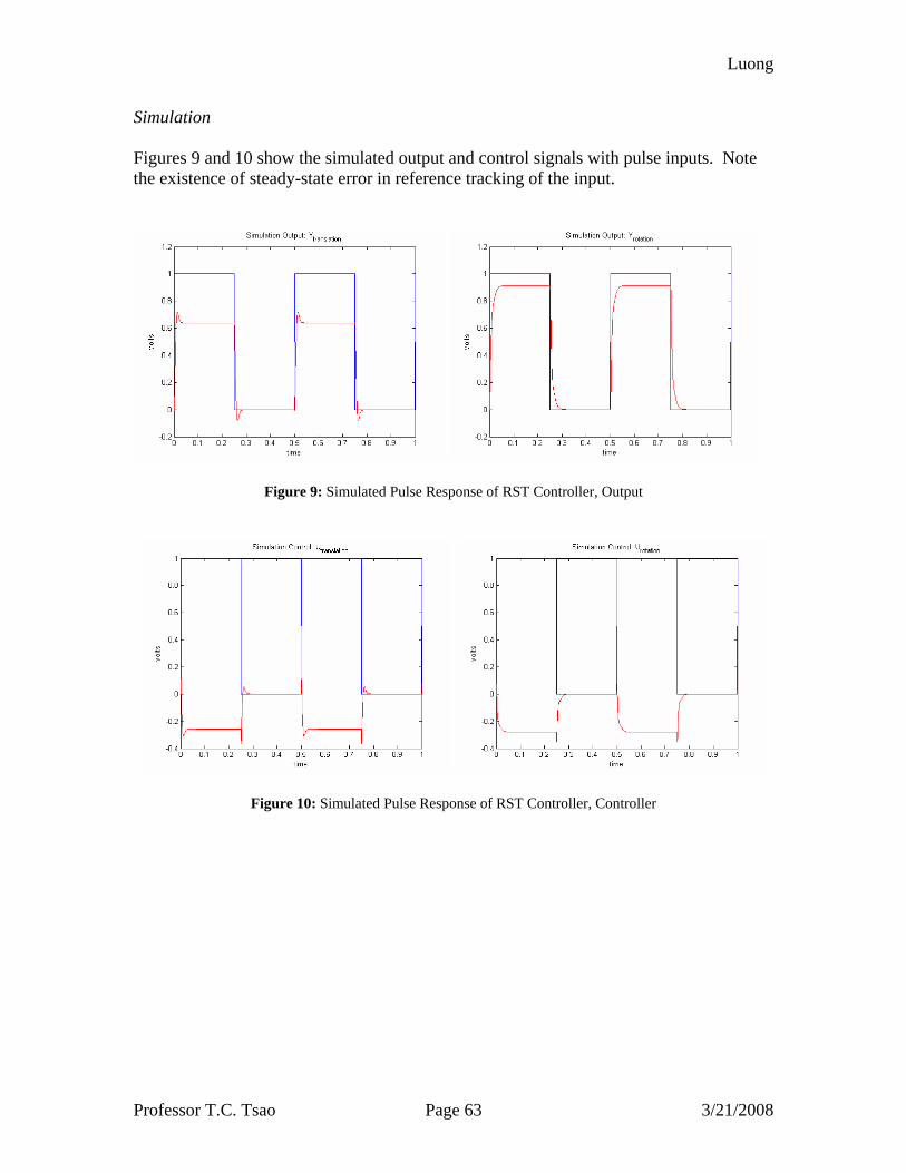
Luong
Professor T.C. Tsao Page 63 3/21/2008
Simulation Figures 9 and 10 show the simulated output and control signals with pulse inputs. Note the existence of steady-state error in reference tracking of the input.
Figure 9: Simulated Pulse Response of RST Controller, Output
Figure 10: Simulated Pulse Response of RST Controller, Controller
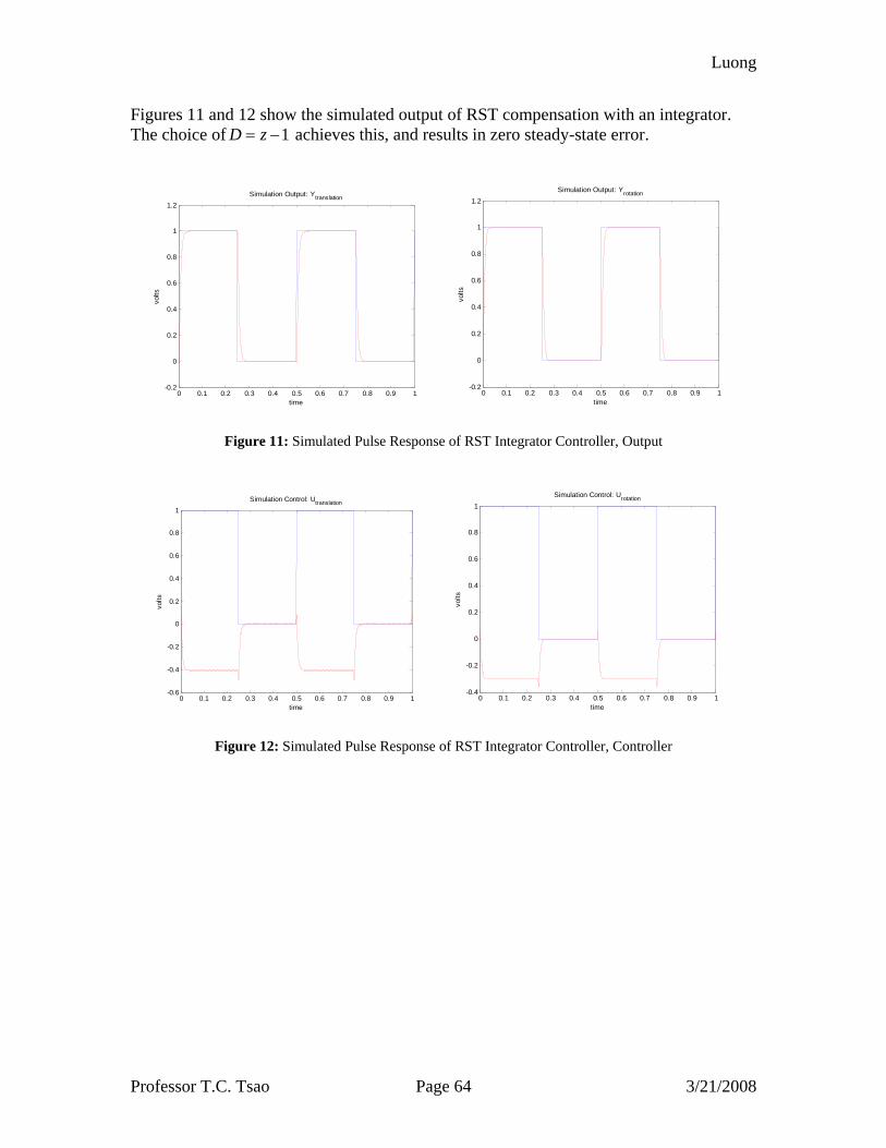
Luong
Professor T.C. Tsao Page 64 3/21/2008
Figures 11 and 12 show the simulated output of RST compensation with an integrator. The choice of 1D z= − achieves this, and results in zero steady-state error.
0 0.1 0.2 0.3 0.4 0.5 0.6 0.7 0.8 0.9 1-0.2
0
0.2
0.4
0.6
0.8
1
1.2Simulation Output: Ytranslation
time
volts
0 0.1 0.2 0.3 0.4 0.5 0.6 0.7 0.8 0.9 1-0.2
0
0.2
0.4
0.6
0.8
1
1.2Simulation Output: Yrotation
time
volts
Figure 11: Simulated Pulse Response of RST Integrator Controller, Output
0 0.1 0.2 0.3 0.4 0.5 0.6 0.7 0.8 0.9 1-0.6
-0.4
-0.2
0
0.2
0.4
0.6
0.8
1Simulation Control: Utranslation
time
volts
0 0.1 0.2 0.3 0.4 0.5 0.6 0.7 0.8 0.9 1-0.4
-0.2
0
0.2
0.4
0.6
0.8
1Simulation Control: Urotation
time
volts
Figure 12: Simulated Pulse Response of RST Integrator Controller, Controller
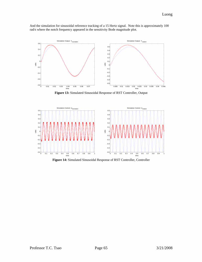
Luong
Professor T.C. Tsao Page 65 3/21/2008
And the simulation for sinusoidal reference tracking of a 15 Hertz signal. Note this is approximately 100 rad/s where the notch frequency appeared in the sensitivity Bode magnitude plot.
0 0.01 0.02 0.03 0.04 0.05 0.06 0.07-0.8
-0.6
-0.4
-0.2
0
0.2
0.4
0.6Simulation Output: Ytranslation
time
volts
0.005 0.01 0.015 0.02 0.025 0.03 0.035 0.04 0.045
-0.5
-0.4
-0.3
-0.2
-0.1
0
0.1
0.2
0.3
0.4
0.5
Simulation Output: Yrotation
time
volts
Figure 13: Simulated Sinusoidal Response of RST Controller, Output
0 0.1 0.2 0.3 0.4 0.5 0.6 0.7 0.8 0.9 1-0.5
-0.4
-0.3
-0.2
-0.1
0
0.1
0.2
0.3
0.4
0.5Simulation Control: Utranslation
time
volts
0 0.1 0.2 0.3 0.4 0.5 0.6 0.7 0.8 0.9 1-0.5
-0.4
-0.3
-0.2
-0.1
0
0.1
0.2
0.3
0.4
0.5Simulation Control: Urotation
time
volts
Figure 14: Simulated Sinusoidal Response of RST Controller, Controller
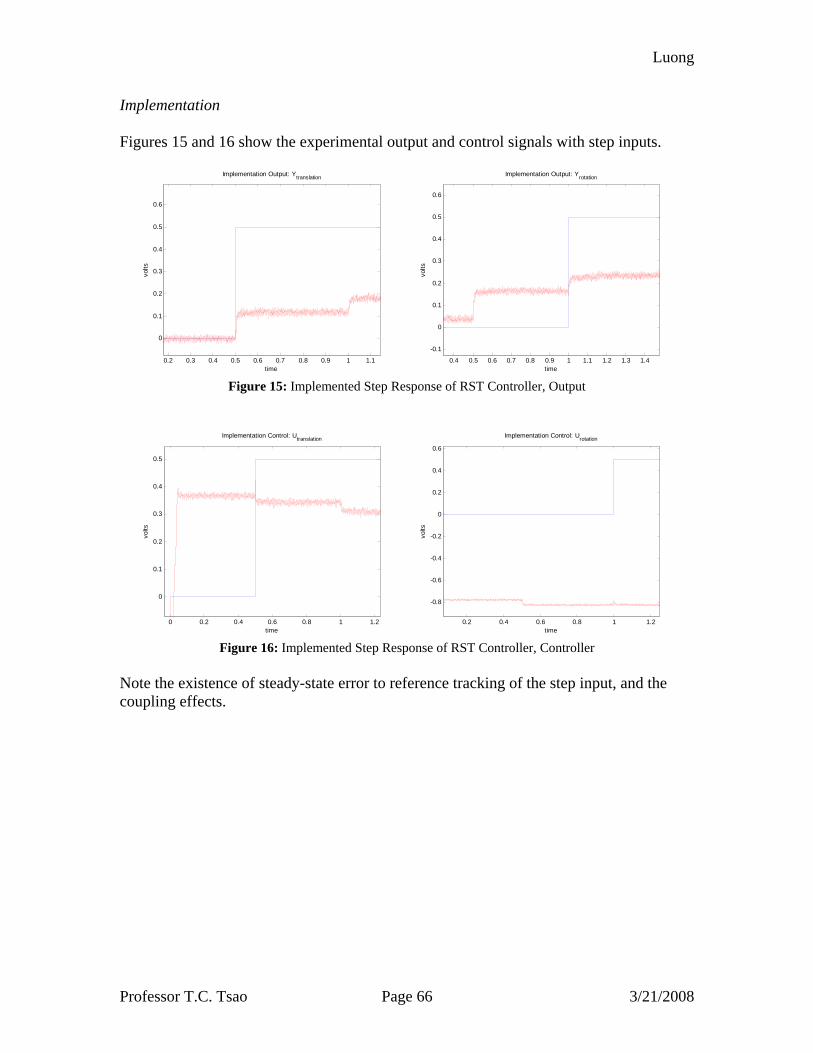
Luong
Professor T.C. Tsao Page 66 3/21/2008
Implementation Figures 15 and 16 show the experimental output and control signals with step inputs.
0.2 0.3 0.4 0.5 0.6 0.7 0.8 0.9 1 1.1
0
0.1
0.2
0.3
0.4
0.5
0.6
Implementation Output: Ytranslation
time
volts
0.4 0.5 0.6 0.7 0.8 0.9 1 1.1 1.2 1.3 1.4
-0.1
0
0.1
0.2
0.3
0.4
0.5
0.6
Implementation Output: Yrotation
time
volts
Figure 15: Implemented Step Response of RST Controller, Output
0 0.2 0.4 0.6 0.8 1 1.2
0
0.1
0.2
0.3
0.4
0.5
Implementation Control: Utranslation
time
volts
0.2 0.4 0.6 0.8 1 1.2
-0.8
-0.6
-0.4
-0.2
0
0.2
0.4
0.6
Implementation Control: Urotation
time
volts
Figure 16: Implemented Step Response of RST Controller, Controller
Note the existence of steady-state error to reference tracking of the step input, and the coupling effects.
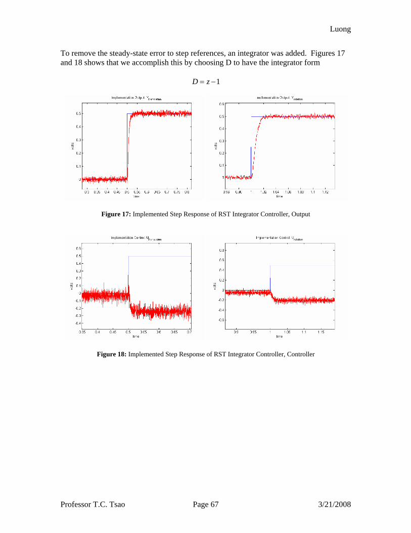
Luong
Professor T.C. Tsao Page 67 3/21/2008
To remove the steady-state error to step references, an integrator was added. Figures 17 and 18 shows that we accomplish this by choosing D to have the integrator form
1D z= −
Figure 17: Implemented Step Response of RST Integrator Controller, Output
Figure 18: Implemented Step Response of RST Integrator Controller, Controller
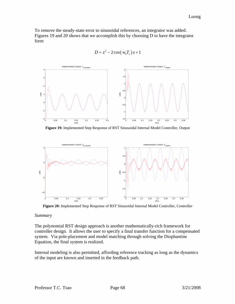
Luong
Professor T.C. Tsao Page 68 3/21/2008
To remove the steady-state error to sinusoidal references, an integrator was added. Figures 19 and 20 shows that we accomplish this by choosing D to have the integrator form
( )202cos 1sD z w T z= − +
0 0.05 0.1 0.15 0.2 0.25 0.3-2
-1
0
1
2
3
4Implementation Output: Ytranslation
time
volts
0 0.05 0.1 0.15 0.2 0.25 0.3 0.35-1.5
-1
-0.5
0
0.5
1
1.5
2Implementation Output: Yrotation
time
volts
Figure 19: Implemented Step Response of RST Sinusoidal Internal Model Controller, Output
0 0.05 0.1 0.15 0.2 0.25
-10
-5
0
5Implementation Control: Utranslation
time
volts
0 0.05 0.1 0.15 0.2 0.25 0.3 0.35-2
-1.5
-1
-0.5
0
0.5
1Implementation Control: Urotation
time
volts
Figure 20: Implemented Step Response of RST Sinusoidal Internal Model Controller, Controller
Summary The polynomial RST design approach is another mathematically-rich framework for controller design. It allows the user to specify a final transfer function for a compensated system. Via pole-placement and model matching through solving the Diophantine Equation, the final system is realized. Internal modeling is also permitted, affording reference tracking as long as the dynamics of the input are known and inserted in the feedback path.
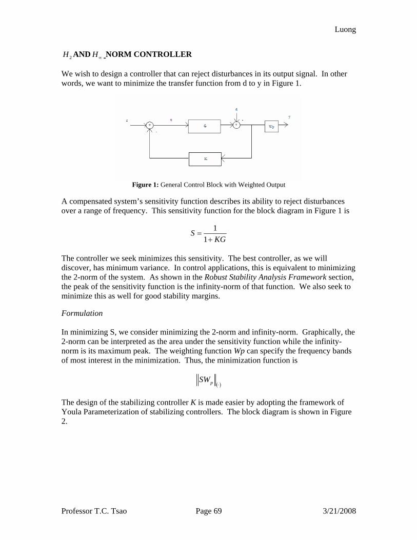
Luong
Professor T.C. Tsao Page 69 3/21/2008
2H AND H∞ NORM CONTROLLER We wish to design a controller that can reject disturbances in its output signal. In other words, we want to minimize the transfer function from d to y in Figure 1.
Figure 1: General Control Block with Weighted Output
A compensated system’s sensitivity function describes its ability to reject disturbances over a range of frequency. This sensitivity function for the block diagram in Figure 1 is
11
SKG
=+
The controller we seek minimizes this sensitivity. The best controller, as we will discover, has minimum variance. In control applications, this is equivalent to minimizing the 2-norm of the system. As shown in the Robust Stability Analysis Framework section, the peak of the sensitivity function is the infinity-norm of that function. We also seek to minimize this as well for good stability margins.
Formulation In minimizing S, we consider minimizing the 2-norm and infinity-norm. Graphically, the 2-norm can be interpreted as the area under the sensitivity function while the infinity-norm is its maximum peak. The weighting function Wp can specify the frequency bands of most interest in the minimization. Thus, the minimization function is
( )pSW⋅
The design of the stabilizing controller K is made easier by adopting the framework of Youla Parameterization of stabilizing controllers. The block diagram is shown in Figure 2.
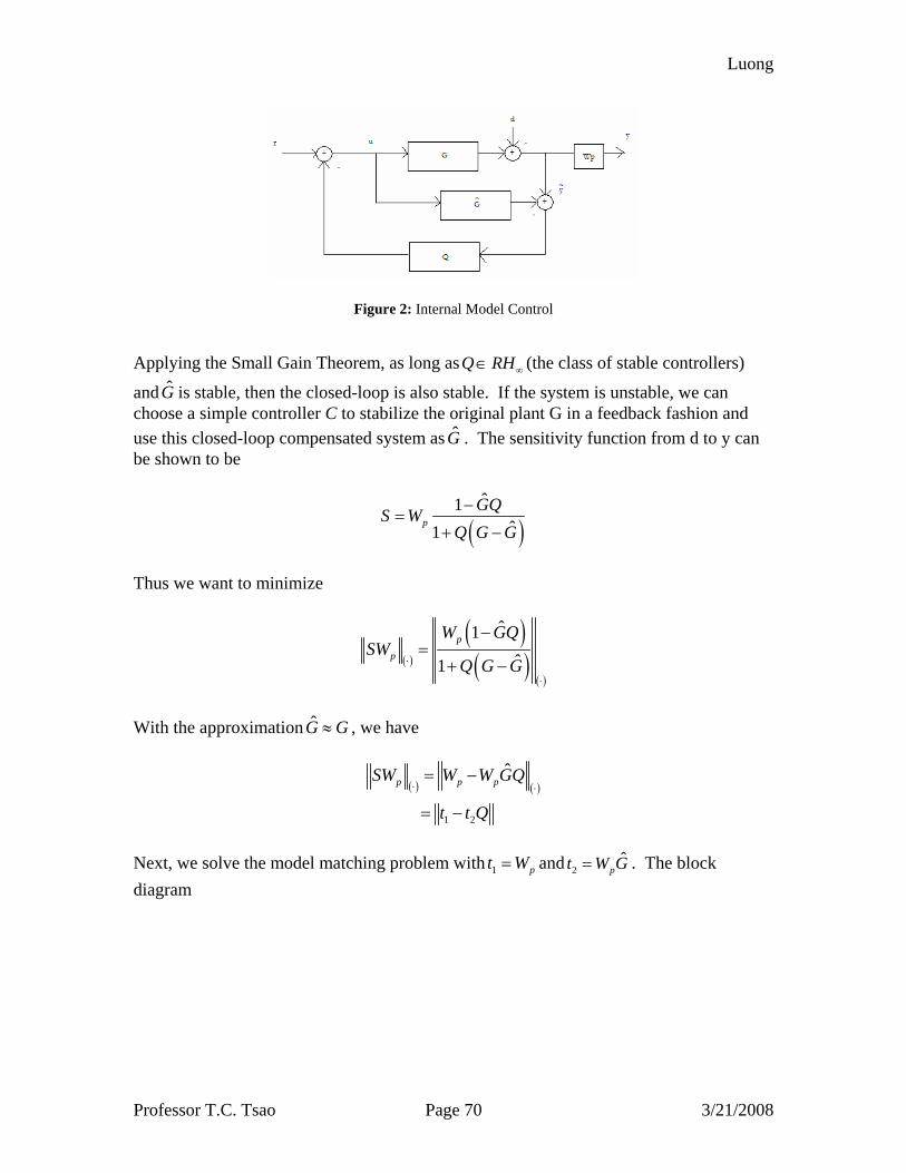
Luong
Professor T.C. Tsao Page 70 3/21/2008
Figure 2: Internal Model Control
Applying the Small Gain Theorem, as long asQ RH∞∈ (the class of stable controllers)
and G is stable, then the closed-loop is also stable. If the system is unstable, we can choose a simple controller C to stabilize the original plant G in a feedback fashion and use this closed-loop compensated system as G . The sensitivity function from d to y can be shown to be
( )ˆ1
ˆ1p
GQS WQ G G−
=+ −
Thus we want to minimize
( )
( )( )
( )
ˆ1ˆ1
pp
W GQSW
Q G G⋅
⋅
−=
+ −
With the approximation G G≈ , we have
( ) ( )
1 2
ˆp p pSW W W GQ
t t Q⋅ ⋅= −
= −
Next, we solve the model matching problem with 1 pt W= and 2
ˆpt W G= . The block
diagram
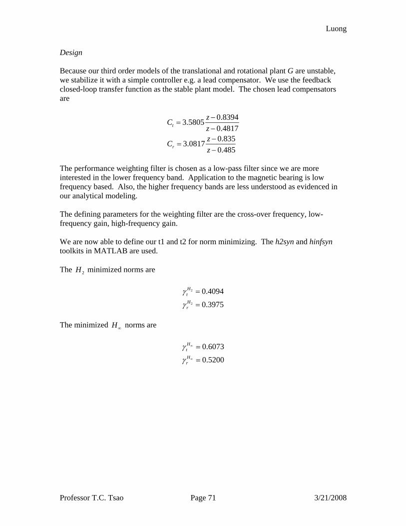
Luong
Professor T.C. Tsao Page 71 3/21/2008
Design Because our third order models of the translational and rotational plant G are unstable, we stabilize it with a simple controller e.g. a lead compensator. We use the feedback closed-loop transfer function as the stable plant model. The chosen lead compensators are
0.83943.58050.48170.8353.08170.485
t
r
zCzzCz
−=
−−
=−
The performance weighting filter is chosen as a low-pass filter since we are more interested in the lower frequency band. Application to the magnetic bearing is low frequency based. Also, the higher frequency bands are less understood as evidenced in our analytical modeling. The defining parameters for the weighting filter are the cross-over frequency, low- frequency gain, high-frequency gain. We are now able to define our t1 and t2 for norm minimizing. The h2syn and hinfsyn toolkits in MATLAB are used. The 2H minimized norms are
2
2
0.4094
0.3975
Ht
Hr
γ
γ
=
=
The minimized H∞ norms are
0.6073
0.5200
HtHr
γ
γ
∞
∞
=
=
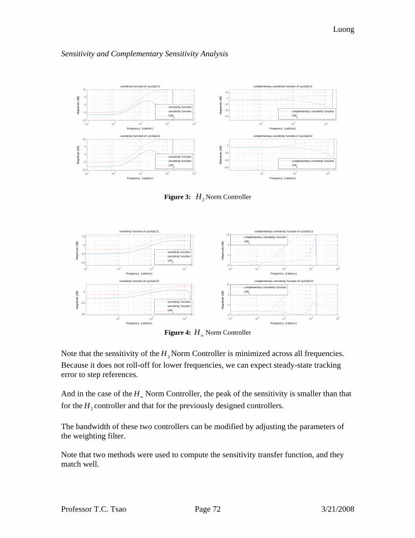
Luong
Professor T.C. Tsao Page 72 3/21/2008
Sensitivity and Complementary Sensitivity Analysis
101
102
103
104
105
-10
-5
0
5
10
Mag
nitu
de (d
B)
sensitivity function of sysGdz11
Frequency (rad/sec)
sensitivity functionsensitivity function1/W
p
101
102
103
104
105
-10
-5
0
5
10
Mag
nitu
de (d
B)
sensitivity function of sysGdz22
Frequency (rad/sec)
sensitivity functionsensitivity function1/W
p
102
103
104
-60
-40
-20
0
20
Mag
nitu
de (d
B)
complementary sensitivity function of sysGdz11
Frequency (rad/sec)
complementary sensitivity function1/W
p
102
103
104
-60
-40
-20
0
Mag
nitu
de (d
B)
complementary sensitivity function of sysGdz22
Frequency (rad/sec)
complementary sensitivity function1/W
p
Figure 3: 2H Norm Controller
101
102
103
104
-20
-10
0
10
Mag
nitu
de (d
B)
sensitivity function of sysGdz11
Frequency (rad/sec)
sensitivity functionsensitivity function1/W
p
102
103
104
-40
-20
0
Mag
nitu
de (d
B)
sensitivity function of sysGdz22
Frequency (rad/sec)
sensitivity functionsensitivity function1/W
p
101
102
103
104
105
-5
0
5
10
Mag
nitu
de (d
B)
complementary sensitivity function of sysGdz11
Frequency (rad/sec)
complementary sensitivity function1/W
p
101
102
103
104
105
-5
0
5
10
Mag
nitu
de (d
B)
complementary sensitivity function of sysGdz22
Frequency (rad/sec)
complementary sensitivity function1/W
p
Figure 4: H∞ Norm Controller
Note that the sensitivity of the 2H Norm Controller is minimized across all frequencies. Because it does not roll-off for lower frequencies, we can expect steady-state tracking error to step references. And in the case of the H∞ Norm Controller, the peak of the sensitivity is smaller than that for the 2H controller and that for the previously designed controllers. The bandwidth of these two controllers can be modified by adjusting the parameters of the weighting filter. Note that two methods were used to compute the sensitivity transfer function, and they match well.
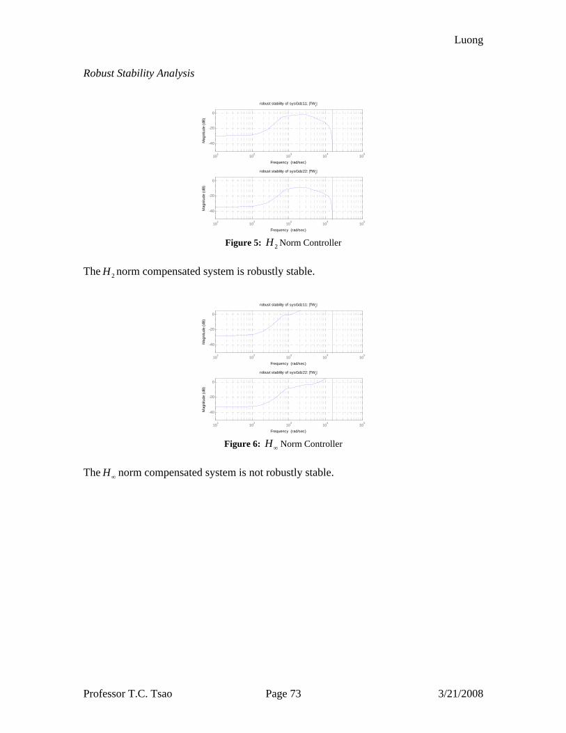
Luong
Professor T.C. Tsao Page 73 3/21/2008
Robust Stability Analysis
101
102
103
104
105
-40
-20
0
Mag
nitu
de (d
B)
robust stability of sysGdz11: |TWr|
Frequency (rad/sec)
101
102
103
104
105
-40
-20
0
Mag
nitu
de (d
B)
robust stability of sysGdz22: |TWr|
Frequency (rad/sec) Figure 5: 2H Norm Controller
The 2H norm compensated system is robustly stable.
101
102
103
104
105
-40
-20
0
Mag
nitu
de (d
B)
robust stability of sysGdz11: |TWr|
Frequency (rad/sec)
101
102
103
104
105
-40
-20
0
Mag
nitu
de (d
B)
robust stability of sysGdz22: |TWr|
Frequency (rad/sec) Figure 6: H∞ Norm Controller
The H∞ norm compensated system is not robustly stable.
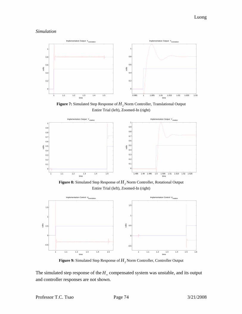
Luong
Professor T.C. Tsao Page 74 3/21/2008
Simulation
1 1.1 1.2 1.3 1.4 1.5
0
0.2
0.4
0.6
0.8
1
Implementation Output: Ytranslation
time
volts
0.995 1 1.005 1.01 1.015 1.02 1.025 1.03
0
0.2
0.4
0.6
0.8
1
Implementation Output: Ytranslation
time
volts
Figure 7: Simulated Step Response of 2H Norm Controller, Translational Output
Entire Trial (left), Zoomed-In (right)
1 1.1 1.2 1.3 1.4 1.5
0
0.1
0.2
0.3
0.4
0.5
0.6
0.7
0.8
0.9
1
Implementation Output: Yrotation
time
volts
1.485 1.49 1.495 1.5 1.505 1.51 1.515 1.52 1.525
0
0.1
0.2
0.3
0.4
0.5
0.6
0.7
0.8
0.9
1
Implementation Output: Yrotation
time
volts
Figure 8: Simulated Step Response of 2H Norm Controller, Rotational Output
Entire Trial (left), Zoomed-In (right)
1 1.1 1.2 1.3 1.4 1.5
-0.5
0
0.5
1
1.5
Implementation Control: Utranslation
time
volts
1 1.1 1.2 1.3 1.4 1.5 1.6
-0.5
0
0.5
1
1.5
Implementation Control: Urotation
time
volts
Figure 9: Simulated Step Response of 2H Norm Controller, Controller Output
The simulated step response of the H∞ compensated system was unstable, and its output and controller responses are not shown.
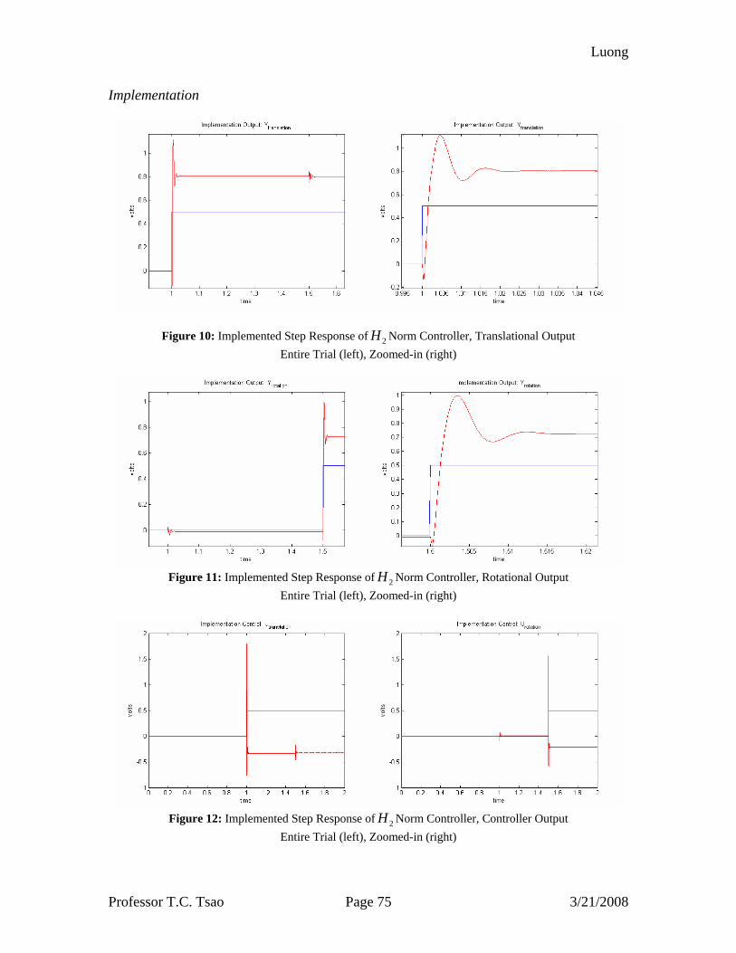
Luong
Professor T.C. Tsao Page 75 3/21/2008
Implementation
Figure 10: Implemented Step Response of 2H Norm Controller, Translational Output Entire Trial (left), Zoomed-in (right)
Figure 11: Implemented Step Response of 2H Norm Controller, Rotational Output
Entire Trial (left), Zoomed-in (right)
Figure 12: Implemented Step Response of 2H Norm Controller, Controller Output
Entire Trial (left), Zoomed-in (right)

Luong
Professor T.C. Tsao Page 76 3/21/2008
Summary From the Youla Parameterization of the class of all stabilizing controllers, the 2H and H∞ controllers were selected based on a selected criteria to minimize.
The 2H norm controller has its advantage in that it minimizes the ratio of the output power to disturbance power. Thus, we expect this system to perform the best of all controllers in the stabilizing class in the presence of output disturbance. The H∞ norm controller minimizes the peak of the sensitivity function, and produces a system with the best stability margins. Note that reference tracking is not possible in these two controllers since the minimization of the sensitivity function is over all frequencies.
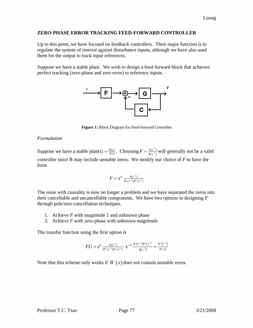
Luong
Professor T.C. Tsao Page 77 3/21/2008
ZERO-PHASE ERROR TRACKING FEED-FORWARD CONTROLLER Up to this point, we have focused on feedback controllers. Their major function is to regulate the system of interest against disturbance inputs, although we have also used them for the output to track input references. Suppose we have a stable plant. We wish to design a feed-forward block that achieves perfect tracking (zero-phase and zero error) to reference inputs.
Figure 1: Block Diagram for Feed-forward Controller
Formulation Suppose we have a stable plant ( )
( )B zA zG = . Choosing
1
1( )( )
A zB z
F−
−= will generally not be a valid
controller since B may include unstable zeros. We modify our choice of F to have the form
1
1 1( )
( ) ( )A zd
B z B zF z
−
+ − − −=
The issue with causality is now no longer a problem and we have separated the zeros into their cancellable and uncancellable components. We have two options in designing F through pole/zero cancellation techniques.
1. Achieve F with magnitude 1 and unknown phase 2. Achieve F with zero-phase with unknown magnitude
The transfer function using the first option is
( ) ( )( )
( )( )
1 1 11
1 1 1( )
( ) ( )
B z B z B zA zd dB z B z B zA z
FG z z+ − − − − −−
+ − − − −−
−= ⋅ =
Note that this scheme only works if ( )B z− does not contain unstable zeros.

Luong
Professor T.C. Tsao Page 78 3/21/2008
The transfer function using the second option relies on the fact that the product of a number and its complex conjugate produces a real result, i.e. zero-phase.
( ) ( )( )
( )1 1 11
1 1
( )( ) ( )( )
B z B z B z B zA z B zd dB z A z
FG z zγ γ
+ − − − − − −− −
+ − −
−= ⋅ ⋅ =
By choosing gamma appropriately, we can achieve DC gain of 1, and approximately so for lower frequencies.
( )( )21Bγ −=
Note the tracking performance at low frequencies is typically better compared to higher frequencies. At other frequencies, the magnitude can be different than the DC gain. However, we can choose gamma in such a way that the gain at a particular frequency is 1, and achieve tracking for references containing that frequency.
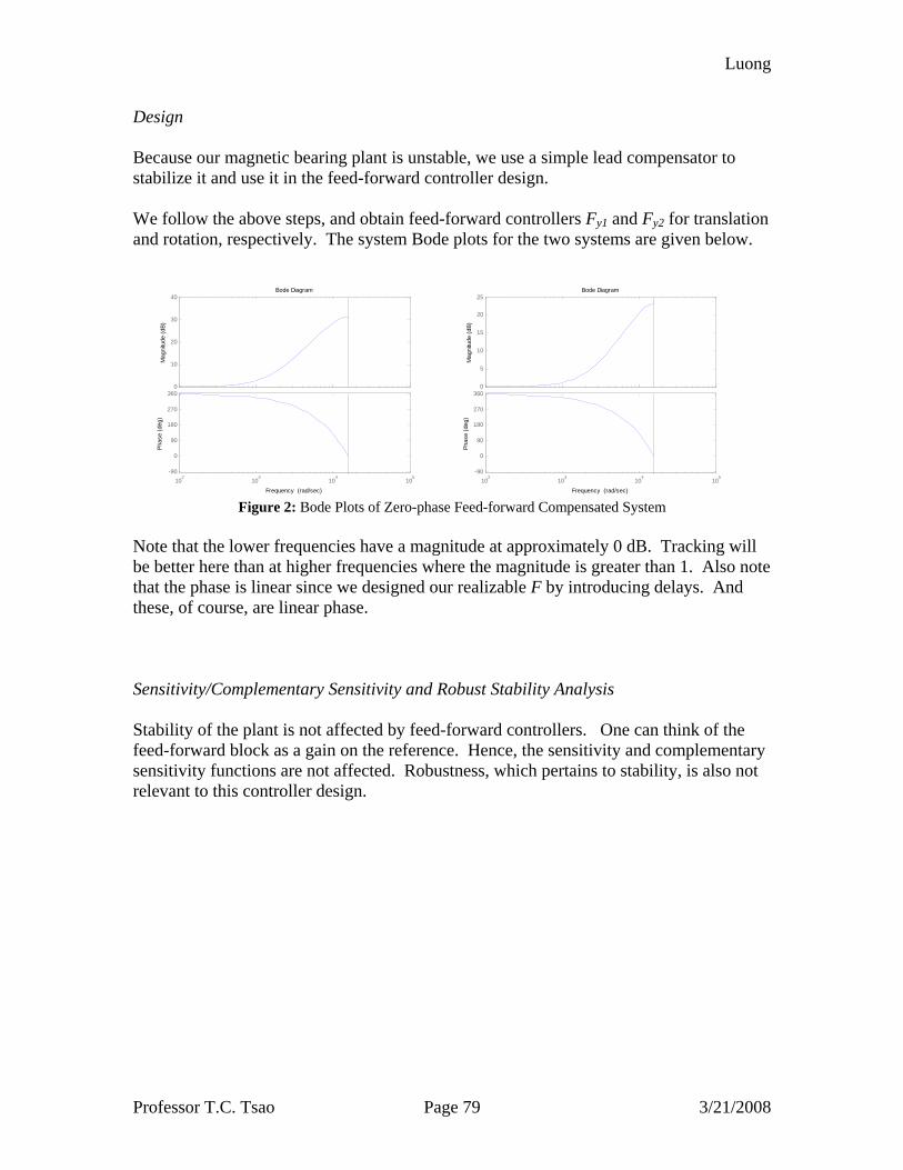
Luong
Professor T.C. Tsao Page 79 3/21/2008
Design Because our magnetic bearing plant is unstable, we use a simple lead compensator to stabilize it and use it in the feed-forward controller design. We follow the above steps, and obtain feed-forward controllers Fy1 and Fy2 for translation and rotation, respectively. The system Bode plots for the two systems are given below.
0
10
20
30
40
Mag
nitu
de (d
B)
102
103
104
105
-90
0
90
180
270
360
Phas
e (d
eg)
Bode Diagram
Frequency (rad/sec)
0
5
10
15
20
25
Mag
nitu
de (d
B)
102
103
104
105
-90
0
90
180
270
360
Phas
e (d
eg)
Bode Diagram
Frequency (rad/sec) Figure 2: Bode Plots of Zero-phase Feed-forward Compensated System
Note that the lower frequencies have a magnitude at approximately 0 dB. Tracking will be better here than at higher frequencies where the magnitude is greater than 1. Also note that the phase is linear since we designed our realizable F by introducing delays. And these, of course, are linear phase. Sensitivity/Complementary Sensitivity and Robust Stability Analysis Stability of the plant is not affected by feed-forward controllers. One can think of the feed-forward block as a gain on the reference. Hence, the sensitivity and complementary sensitivity functions are not affected. Robustness, which pertains to stability, is also not relevant to this controller design.
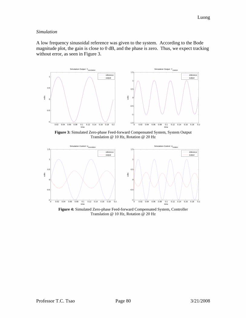
Luong
Professor T.C. Tsao Page 80 3/21/2008
Simulation A low frequency sinusoidal reference was given to the system. According to the Bode magnitude plot, the gain is close to 0 dB, and the phase is zero. Thus, we expect tracking without error, as seen in Figure 3.
0.02 0.04 0.06 0.08 0.1 0.12 0.14 0.16 0.18 0.2-1
-0.5
0
0.5
1
Simulation Output: Ytranslation
time
volts
referenceoutput
0 0.02 0.04 0.06 0.08 0.1 0.12 0.14 0.16 0.18 0.2-1.5
-1
-0.5
0
0.5
1
1.5Simulation Output: Yrotation
timevo
lts
referenceoutput
Figure 3: Simulated Zero-phase Feed-forward Compensated System, System Output
Translation @ 10 Hz, Rotation @ 20 Hz
0 0.02 0.04 0.06 0.08 0.1 0.12 0.14 0.16 0.18 0.2-1
-0.5
0
0.5
1
1.5Simulation Control: Utranslation
time
volts
referenceoutput
0 0.02 0.04 0.06 0.08 0.1 0.12 0.14 0.16 0.18 0.2-1
-0.5
0
0.5
1
1.5Simulation Control: Urotation
time
volts
referenceoutput
Figure 4: Simulated Zero-phase Feed-forward Compensated System, Controller
Translation @ 10 Hz, Rotation @ 20 Hz
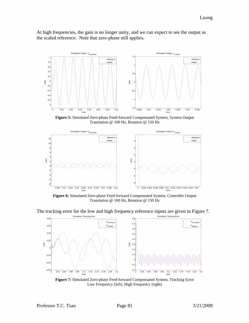
Luong
Professor T.C. Tsao Page 81 3/21/2008
At high frequencies, the gain is no longer unity, and we can expect to see the output as the scaled reference. Note that zero-phase still applies.
0 0.01 0.02 0.03 0.04 0.05 0.06 0.07
-1
-0.8
-0.6
-0.4
-0.2
0
0.2
0.4
0.6
0.8
1
Simulation Output: Ytranslation
time
volts
referenceoutput
0.005 0.01 0.015 0.02 0.025 0.03 0.035-1.5
-1
-0.5
0
0.5
1
1.5Simulation Output: Yrotation
time
volts
referenceoutput
Figure 5: Simulated Zero-phase Feed-forward Compensated System, System Output
Translation @ 100 Hz, Rotation @ 150 Hz
0.005 0.01 0.015 0.02 0.025 0.03 0.035 0.04 0.045 0.05
-8
-6
-4
-2
0
2
4
6
8
10
12
Simulation Control: Utranslation
time
volts
referenceoutput
0 0.002 0.004 0.006 0.008 0.01 0.012 0.014 0.016 0.018 0.02
-4
-2
0
2
4
6
8
Simulation Control: Urotation
time
volts
referenceoutput
Figure 6: Simulated Zero-phase Feed-forward Compensated System, Controller Output
Translation @ 100 Hz, Rotation @ 150 Hz
The tracking error for the low and high frequency reference inputs are given in Figure 7.
0 0.02 0.04 0.06 0.08 0.1 0.12 0.14 0.16 0.18 0.2-0.06
-0.04
-0.02
0
0.02
0.04
0.06
0.08Simulation Tracking Error
time
volts
etranslation
eRotation
0 0.02 0.04 0.06 0.08 0.1 0.12 0.14 0.16 0.18 0.2-0.2
-0.1
0
0.1
0.2
0.3
0.4
0.5
0.6
0.7
0.8Simulation Tracking Error
time
volts
etranslation
eRotation
Figure 7: Simulated Zero-phase Feed-forward Compensated System, Tracking Error
Low Frequency (left), High Frequency (right)
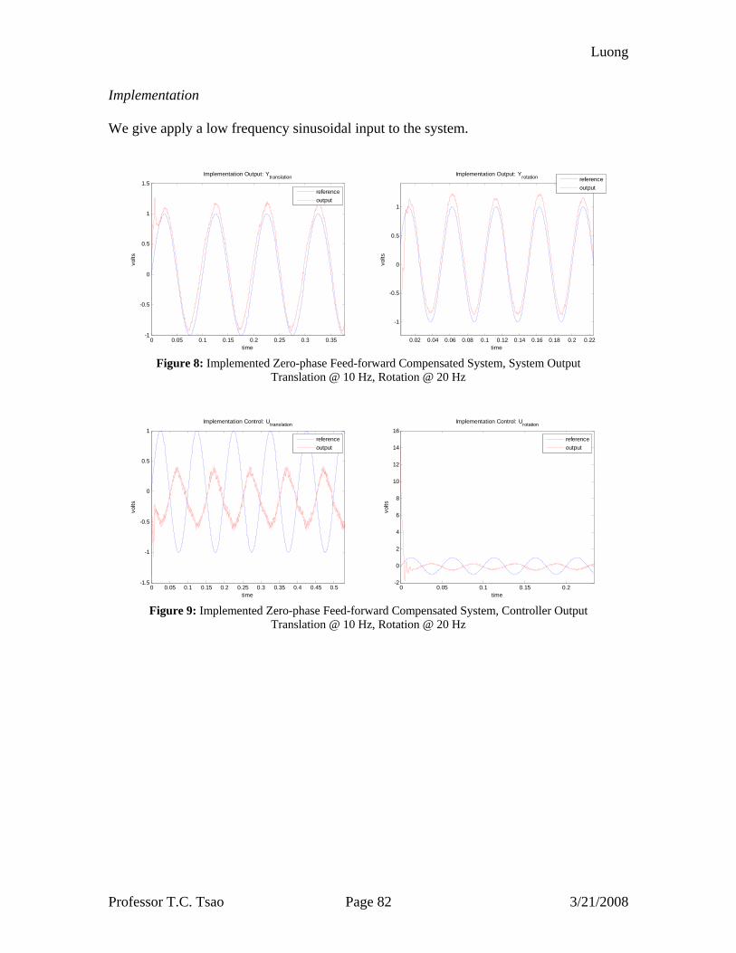
Luong
Professor T.C. Tsao Page 82 3/21/2008
Implementation We give apply a low frequency sinusoidal input to the system.
0 0.05 0.1 0.15 0.2 0.25 0.3 0.35-1
-0.5
0
0.5
1
1.5Implementation Output: Ytranslation
time
volts
referenceoutput
0.02 0.04 0.06 0.08 0.1 0.12 0.14 0.16 0.18 0.2 0.22
-1
-0.5
0
0.5
1
Implementation Output: Yrotation
time
volts
referenceoutput
Figure 8: Implemented Zero-phase Feed-forward Compensated System, System Output
Translation @ 10 Hz, Rotation @ 20 Hz
0 0.05 0.1 0.15 0.2 0.25 0.3 0.35 0.4 0.45 0.5-1.5
-1
-0.5
0
0.5
1Implementation Control: Utranslation
time
volts
referenceoutput
0 0.05 0.1 0.15 0.2-2
0
2
4
6
8
10
12
14
16Implementation Control: Urotation
time
volts
referenceoutput
Figure 9: Implemented Zero-phase Feed-forward Compensated System, Controller Output
Translation @ 10 Hz, Rotation @ 20 Hz
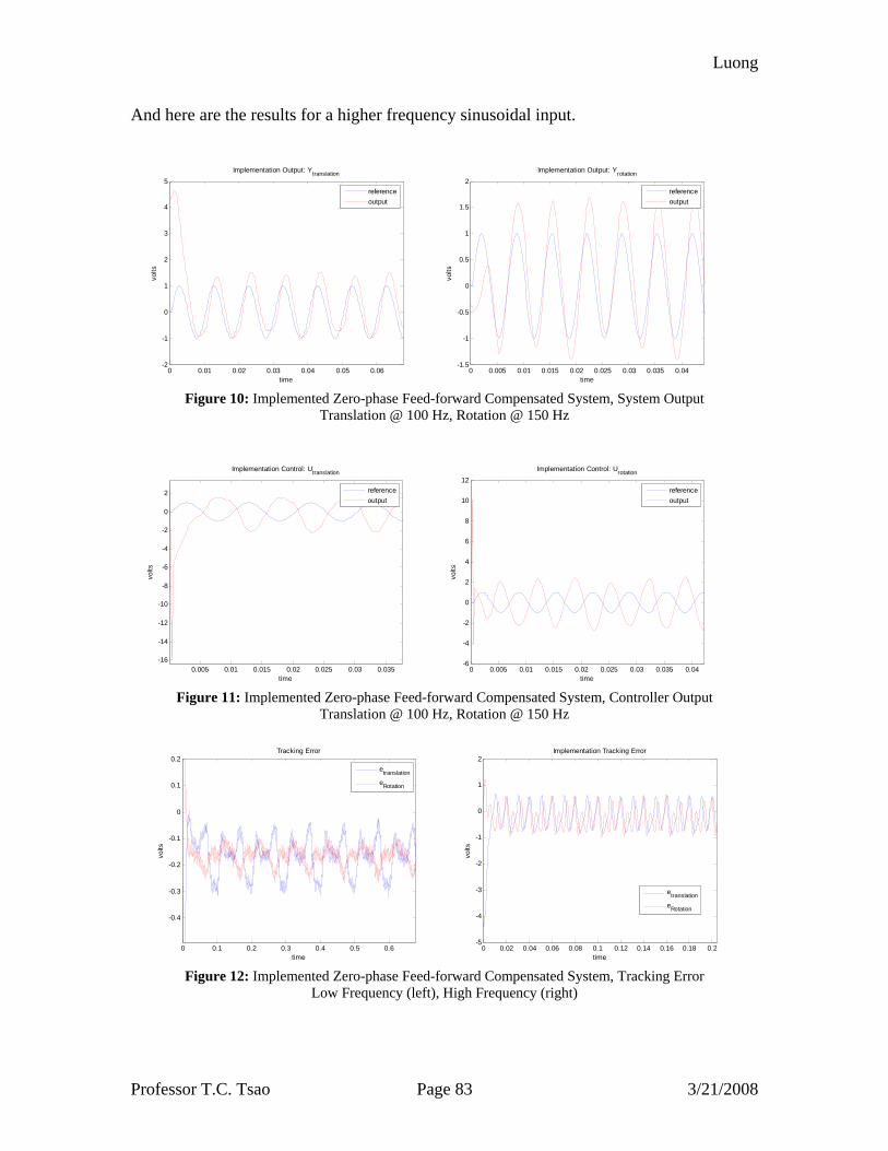
Luong
Professor T.C. Tsao Page 83 3/21/2008
And here are the results for a higher frequency sinusoidal input.
0 0.01 0.02 0.03 0.04 0.05 0.06-2
-1
0
1
2
3
4
5Implementation Output: Ytranslation
time
volts
referenceoutput
0 0.005 0.01 0.015 0.02 0.025 0.03 0.035 0.04-1.5
-1
-0.5
0
0.5
1
1.5
2Implementation Output: Yrotation
time
volts
referenceoutput
Figure 10: Implemented Zero-phase Feed-forward Compensated System, System Output
Translation @ 100 Hz, Rotation @ 150 Hz
0.005 0.01 0.015 0.02 0.025 0.03 0.035-16
-14
-12
-10
-8
-6
-4
-2
0
2
Implementation Control: Utranslation
time
volts
referenceoutput
0 0.005 0.01 0.015 0.02 0.025 0.03 0.035 0.04-6
-4
-2
0
2
4
6
8
10
12Implementation Control: Urotation
time
volts
referenceoutput
Figure 11: Implemented Zero-phase Feed-forward Compensated System, Controller Output
Translation @ 100 Hz, Rotation @ 150 Hz
0 0.1 0.2 0.3 0.4 0.5 0.6
-0.4
-0.3
-0.2
-0.1
0
0.1
0.2Tracking Error
time
volts
etranslation
eRotation
0 0.02 0.04 0.06 0.08 0.1 0.12 0.14 0.16 0.18 0.2-5
-4
-3
-2
-1
0
1
2Implementation Tracking Error
time
volts
etranslation
eRotation
Figure 12: Implemented Zero-phase Feed-forward Compensated System, Tracking Error
Low Frequency (left), High Frequency (right)

Luong
Professor T.C. Tsao Page 84 3/21/2008
Summary We achieve better tracking of a reference through the design of a zero-phase controller that inverts the dynamics of the plant. It is important we know the plant well to ensure this tracking, i.e. the pole and zero locations, as they were relied on in the controller formulation. The advantage of this design is that it is relatively simple compared to the other more mathematically rigorous controllers. The feed-forward feature of this design eliminates the need for feedback that has effects on stability and robustness. As long as the plant is stable, we can achieve near perfect tracking with the simple zero-phase feed-forward controller.
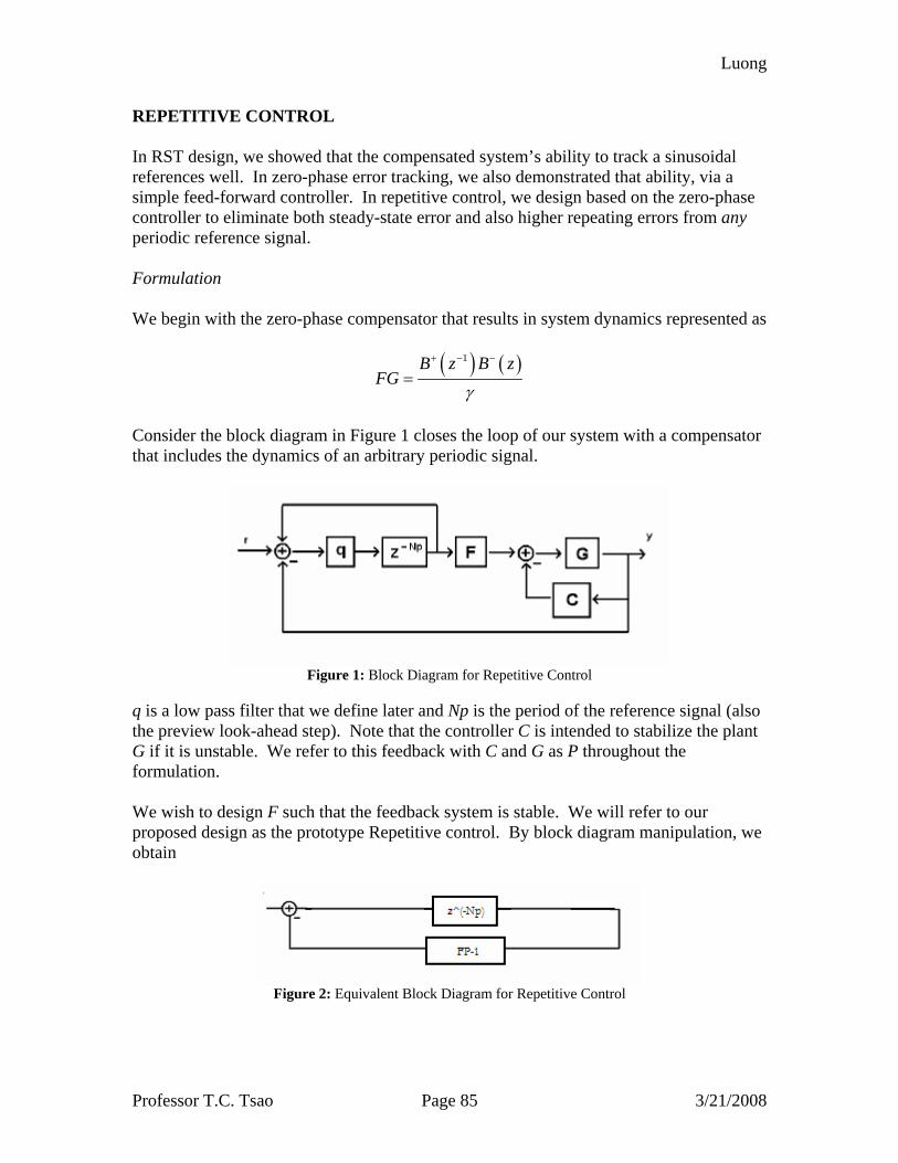
Luong
Professor T.C. Tsao Page 85 3/21/2008
REPETITIVE CONTROL In RST design, we showed that the compensated system’s ability to track a sinusoidal references well. In zero-phase error tracking, we also demonstrated that ability, via a simple feed-forward controller. In repetitive control, we design based on the zero-phase controller to eliminate both steady-state error and also higher repeating errors from any periodic reference signal. Formulation We begin with the zero-phase compensator that results in system dynamics represented as
( ) ( )1B z B zFG
γ
+ − −
=
Consider the block diagram in Figure 1 closes the loop of our system with a compensator that includes the dynamics of an arbitrary periodic signal.
Figure 1: Block Diagram for Repetitive Control
q is a low pass filter that we define later and Np is the period of the reference signal (also the preview look-ahead step). Note that the controller C is intended to stabilize the plant G if it is unstable. We refer to this feedback with C and G as P throughout the formulation. We wish to design F such that the feedback system is stable. We will refer to our proposed design as the prototype Repetitive control. By block diagram manipulation, we obtain
Figure 2: Equivalent Block Diagram for Repetitive Control
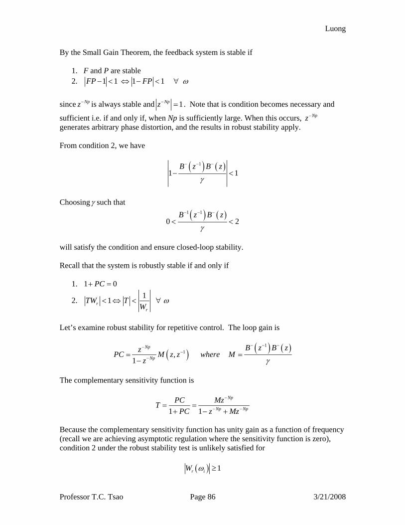
Luong
Professor T.C. Tsao Page 86 3/21/2008
By the Small Gain Theorem, the feedback system is stable if
1. F and P are stable 2. 1 1 1 1FP FP ω− < ⇔ − < ∀
since Npz− is always stable and 1Npz− = . Note that is condition becomes necessary and
sufficient i.e. if and only if, when Np is sufficiently large. When this occurs, Npz− generates arbitrary phase distortion, and the results in robust stability apply. From condition 2, we have
( ) ( )1
1 1B z B z
γ
− − −
− <
Choosingγ such that
( ) ( )1 1
0 2B z B z
γ
− − −
< <
will satisfy the condition and ensure closed-loop stability. Recall that the system is robustly stable if and only if
1. 1 0PC+ =
2. 11rr
TW TW
ω< ⇔ < ∀
Let’s examine robust stability for repetitive control. The loop gain is
( ) ( ) ( )11,
1
Np
Np
B z B zzPC M z z where Mz γ
− − −−−
−= =−
The complementary sensitivity function is
1 1
Np
Np Np
PC MzTPC z Mz
−
− −= =+ − +
Because the complementary sensitivity function has unity gain as a function of frequency (recall we are achieving asymptotic regulation where the sensitivity function is zero), condition 2 under the robust stability test is unlikely satisfied for
( ) 1r iW ω ≥
Luong
Professor T.C. Tsao Page 87 3/21/2008
Typical uncertainty bounds, as in the case of our magnetic bearing, have high gain for higher frequencies. Hence, it can be concluded that the proposed repetitive controller is not robustly stable from the high-gain feedback at high frequencies. Seeking a robustly stable controller, we make a modification by introducing a zero-phase low-pass filter Q. The rationale for this choice is our frequency range of interest is on the lower side and our desire for no phase distortion to performance i.e. the sensitivity function. The controller is now
( ) ( )( ) ( )
11 1
1
,
1 ,
Np
Np
Q z z zC z F z
Q z z z
− −− −
− −=
−
Q is restricted to have less than unity magnitude. The performance of this controller is given by the sensitivity function
1 11 1
Np
Np Np
QzSPC Qz MQz
−
− −
−= =
+ − +
and the robust stability measure is
1 1 ( 1)
Np
Np
PC MQzTPC M Qz
−
−= =+ + −
With this T, we wish to design the filter Q such that condition 2 of the robust stability criteria is satisfied. It can be shown that if the following three conditions hold, then this condition is satisfied and the system is robustly stable.
0 110 1
1r
r
MQ T
WQ
W
⎫⎪
< ≤ ⎪⎪< ≤ ⇒ <⎬⎪⎪<⎪⎭
For M closer to 1, the system achieves higher performance in terms of faster tracking convergence. However, robust stability is weakened as the magnitude of T increases. For M closer to 0, performance decreases while the system is more robustly stable since the magnitude of T is smaller than one for a higher range of frequencies. This highlights the trade-off between performance and robust stability. Note that for M between 0 and 2, the resulting system is stable, but not robustly stable.
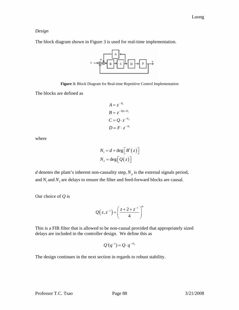
Luong
Professor T.C. Tsao Page 88 3/21/2008
Design The block diagram shown in Figure 3 is used for real-time implementation.
Figure 3: Block Diagram for Real-time Repetitive Control Implementation
The blocks are defined as
1
1
2
1
N
Np N
N
N
A zB zC Q zD F z
−
− +
−
−
=
=
= ⋅
= ⋅
where
( )( )
11
2
deg
deg
N d B z
N Q z
⎡ ⎤= + ⎣ ⎦= ⎡ ⎤⎣ ⎦
d denotes the plant’s inherent non-causality step, pN is the external signals period, and 1N and 2N are delays to ensure the filter and feed-forward blocks are causal.
Our choice of Q is
( )1
1 2,4
mz zQ z z
−− ⎛ ⎞+ +
= ⎜ ⎟⎝ ⎠
This is a FIR filter that is allowed to be non-causal provided that appropriately sized delays are included in the controller design. We define this as
21'( ) NQ q Q q−− = ⋅
The design continues in the next section in regards to robust stability.
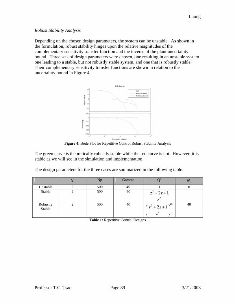
Luong
Professor T.C. Tsao Page 89 3/21/2008
Robust Stability Analysis Depending on the chosen design parameters, the system can be unstable. As shown in the formulation, robust stability hinges upon the relative magnitudes of the complementary sensitivity transfer function and the inverse of the plant uncertainty bound. Three sets of design parameters were chosen, one resulting in an unstable system one leading to a stable, but not robustly stable system, and one that is robustly stable. Their complementary sensitivity transfer functions are shown in relation to the uncertainty bound in Figure 4.
-20
-10
0
10
20
Mag
nitu
de (d
B)
101
102
103
104
105
-5760
-4320
-2880
-1440
0
1440
Phas
e (d
eg)
Bode Diagram
Frequency (rad/sec)
1/WrRobustly StableStablizing Control
Figure 4: Bode Plot for Repetitive Control Robust Stability Analysis
The green curve is theoretically robustly stable while the red curve is not. However, it is stable as we will see in the simulation and implementation. The design parameters for the three cases are summarized in the following table.
1N Np Gamma Q’
2N Unstable 2 500 40 1 0
Stable 2 500 40 2
2
2 1z zz+ +
Robustly Stable
2 500 40 402
2
2 1z zz
⎛ ⎞+ +⎜ ⎟⎝ ⎠
40
Table 1: Repetitive Control Designs
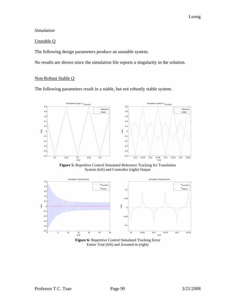
Luong
Professor T.C. Tsao Page 90 3/21/2008
Simulation Unstable Q The following design parameters produce an unstable system. No results are shown since the simulation file reports a singularity in the solution. Non-Robust Stable Q The following parameters result in a stable, but not robustly stable system.
9.4 9.45 9.5 9.55 9.6-0.5
-0.4
-0.3
-0.2
-0.1
0
0.1
0.2
0.3
0.4
0.5Simulation Output: Ytranslation
time
volts
referenceoutput
13.2 13.25 13.3 13.35 13.4 13.45 13.5 13.55-0.5
-0.4
-0.3
-0.2
-0.1
0
0.1
0.2
0.3
0.4
0.5Simulation Control: Utranslation
time
volts
referenceoutput
Figure 5: Repetitive Control Simulated Reference Tracking for Translation
System (left) and Controller (right) Output
0 5 10 15 20 25 30-0.5
-0.4
-0.3
-0.2
-0.1
0
0.1
0.2
0.3
0.4
0.5Simulation Tracking Error
time
volts
etranslation
eRotation
16 16.05 16.1 16.15 16.2 16.25
-0.1
-0.05
0
0.05
0.1
Simulation Tracking Error
time
volts
etranslation
eRotation
Figure 6: Repetitive Control Simulated Tracking Error
Entire Trial (left) and Zoomed-in (right)
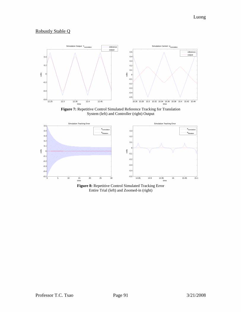
Luong
Professor T.C. Tsao Page 91 3/21/2008
Robustly Stable Q
12.25 12.3 12.35 12.4 12.45-0.6
-0.4
-0.2
0
0.2
0.4
Simulation Output: Ytranslation
time
volts
referenceoutput
10.26 10.28 10.3 10.32 10.34 10.36 10.38 10.4 10.42 10.44
-0.5
-0.4
-0.3
-0.2
-0.1
0
0.1
0.2
0.3
0.4
0.5
Simulation Control: Utranslation
time
volts
referenceoutput
Figure 7: Repetitive Control Simulated Reference Tracking for Translation
System (left) and Controller (right) Output
0 5 10 15 20 25 30-0.5
-0.4
-0.3
-0.2
-0.1
0
0.1
0.2
0.3
0.4
0.5Simulation Tracking Error
time
volts
etranslation
eRotation
14.85 14.9 14.95 15 15.05 15.1
-0.5
-0.4
-0.3
-0.2
-0.1
0
0.1
0.2
0.3
Simulation Tracking Error
time
volts
etranslation
eRotation
Figure 8: Repetitive Control Simulated Tracking Error
Entire Trial (left) and Zoomed-in (right)
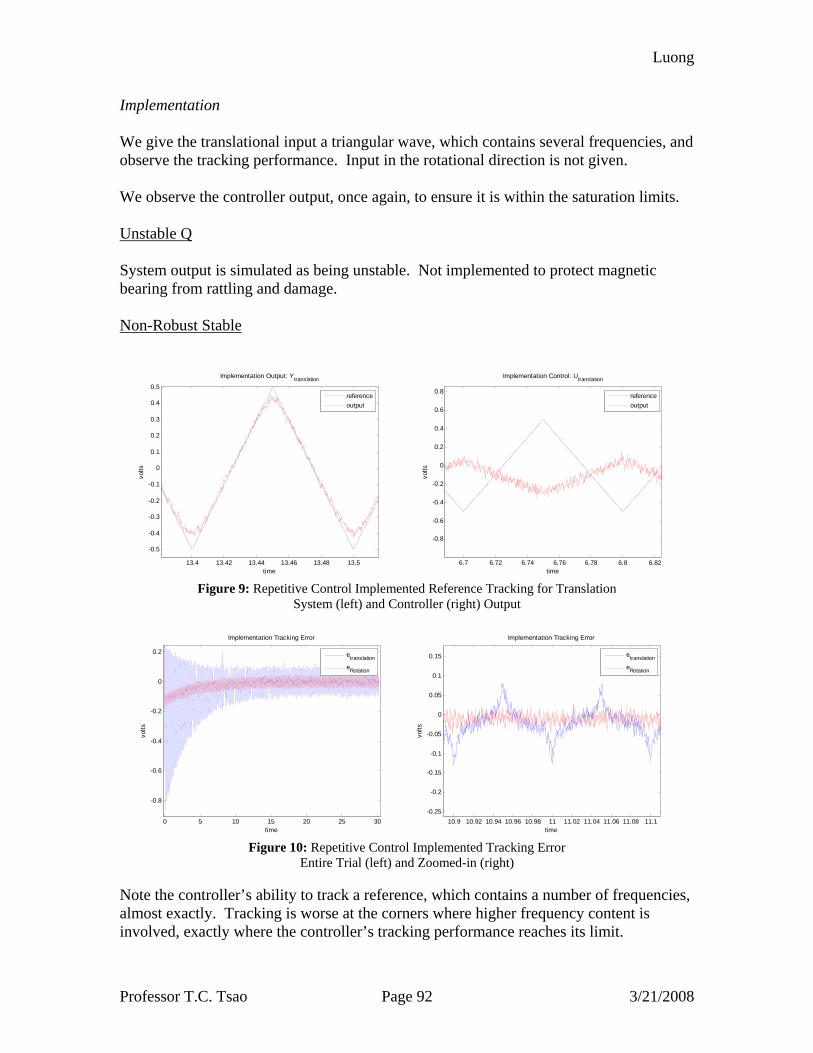
Luong
Professor T.C. Tsao Page 92 3/21/2008
Implementation We give the translational input a triangular wave, which contains several frequencies, and observe the tracking performance. Input in the rotational direction is not given. We observe the controller output, once again, to ensure it is within the saturation limits. Unstable Q System output is simulated as being unstable. Not implemented to protect magnetic bearing from rattling and damage. Non-Robust Stable
13.4 13.42 13.44 13.46 13.48 13.5
-0.5
-0.4
-0.3
-0.2
-0.1
0
0.1
0.2
0.3
0.4
0.5
Implementation Output: Ytranslation
time
volts
referenceoutput
6.7 6.72 6.74 6.76 6.78 6.8 6.82
-0.8
-0.6
-0.4
-0.2
0
0.2
0.4
0.6
0.8
Implementation Control: Utranslation
time
volts
referenceoutput
Figure 9: Repetitive Control Implemented Reference Tracking for Translation
System (left) and Controller (right) Output
0 5 10 15 20 25 30
-0.8
-0.6
-0.4
-0.2
0
0.2
Implementation Tracking Error
time
volts
etranslation
eRotation
10.9 10.92 10.94 10.96 10.98 11 11.02 11.04 11.06 11.08 11.1-0.25
-0.2
-0.15
-0.1
-0.05
0
0.05
0.1
0.15
Implementation Tracking Error
time
volts
etranslation
eRotation
Figure 10: Repetitive Control Implemented Tracking Error
Entire Trial (left) and Zoomed-in (right)
Note the controller’s ability to track a reference, which contains a number of frequencies, almost exactly. Tracking is worse at the corners where higher frequency content is involved, exactly where the controller’s tracking performance reaches its limit.
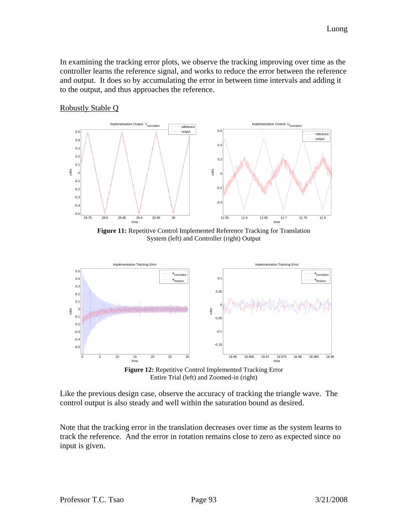
Luong
Professor T.C. Tsao Page 93 3/21/2008
In examining the tracking error plots, we observe the tracking improving over time as the controller learns the reference signal, and works to reduce the error between the reference and output. It does so by accumulating the error in between time intervals and adding it to the output, and thus approaches the reference. Robustly Stable Q
29.75 29.8 29.85 29.9 29.95 30-0.5
-0.4
-0.3
-0.2
-0.1
0
0.1
0.2
0.3
0.4
0.5
Implementation Output: Ytranslation
time
volts
referenceoutput
12.55 12.6 12.65 12.7 12.75 12.8
-0.4
-0.2
0
0.2
0.4
0.6
Implementation Control: Utranslation
time
volts
referenceoutput
Figure 11: Repetitive Control Implemented Reference Tracking for Translation
System (left) and Controller (right) Output
0 5 10 15 20 25 30
-0.5
-0.4
-0.3
-0.2
-0.1
0
0.1
0.2
0.3
0.4
0.5
Implementation Tracking Error
time
volts
etranslation
eRotation
18.96 18.965 18.97 18.975 18.98 18.985 18.99
-0.15
-0.1
-0.05
0
0.05
0.1
Implementation Tracking Error
time
volts
etranslation
eRotation
Figure 12: Repetitive Control Implemented Tracking Error
Entire Trial (left) and Zoomed-in (right)
Like the previous design case, observe the accuracy of tracking the triangle wave. The control output is also steady and well within the saturation bound as desired.
Note that the tracking error in the translation decreases over time as the system learns to track the reference. And the error in rotation remains close to zero as expected since no input is given.

Luong
Professor T.C. Tsao Page 94 3/21/2008
Summary The repetitive controller achieves reference tracking to multiple frequencies, a feat the other controllers in this report did not handle. By using the IMP for any periodic signal, we were able to insert this dynamic into the controller. Although we can insert such periodic dynamics into the RST and state-observer controllers, doing so may prove disastrous in implementation. For periodic signals of high orders, numerical issues arise such as slower computing times, high computation errors, and requires for high-order filters. Repetitive control, on the other hand, effectively handles large orders with ease. This controller is ideal in learning control applications where the reference signal is periodic and known.

Luong
Professor T.C. Tsao Page 95 3/21/2008
APPENDEX
MATLAB FILE FUNCTION system_id
Performs analytical modeling and experimental validation, plant decoupling and uncertainty
lead_lag_design Step responses, Nyquist and Bode Plots state_feedback_observer_full State Estimator Feedback state_feedback_observer_integrator_full Augmented with integrator modelmatch RST Controller dioph Solves the Diophantine Equation RST Solves for R, S, and T via the Diophantine
Equation Youla_example1 H2 and H-inf controller, sensitivity and
robust stability, simulation H2ModelMatching Solves the H2 and H-inf controller via
model matching designZeroPhase Zero-phase Error Tracking Controller zeroPhase Returns transfer function of FF block
resulting in linear phase system designRepControl Repetitive Control
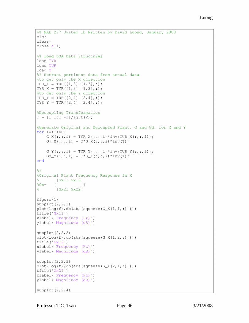
Luong
Professor T.C. Tsao Page 96 3/21/2008
%% MAE 277 System ID Written by David Luong, January 2008 clc; clear; close all; %% Load DSA Data Structures load TYR load TUR load f %% Extract pertinent data from actual data %to get only the X direction TUR_X = TUR([1,3],[1,3],:); TYR_X = TYR([1,3],[1,3],:); %to get only the Y direction TUR_Y = TUR([2,4],[2,4],:); TYR_Y = TYR([2,4],[2,4],:); %Decoupling Transformation T = [1 1;1 -1]/sqrt(2); %Generate Original and Decoupled Plant, G and Gd, for X and Y for i=1:1601 G_X(:,:,i) = TYR_X(:,:,i)*inv(TUR_X(:,:,i)); Gd_X(:,:,i) = T*G_X(:,:,i)*inv(T); G_Y(:,:,i) = TYR_Y(:,:,i)*inv(TUR_Y(:,:,i)); Gd_Y(:,:,i) = T*G_Y(:,:,i)*inv(T); end %% %Original Plant Frequency Response in X % [Gx11 Gx12] %Gx= [ ] % [Gx21 Gx22] figure(1) subplot(2,2,1) plot(log(f),db(abs(squeeze(G_X(1,1,:))))) title('Gx11') xlabel('Frequency (Hz)') ylabel('Magnitude (dB)') subplot(2,2,2) plot(log(f),db(abs(squeeze(G_X(1,2,:))))) title('Gx12') xlabel('Frequency (Hz)') ylabel('Magnitude (dB)') subplot(2,2,3) plot(log(f),db(abs(squeeze(G_X(2,1,:))))) title('Gx21') xlabel('Frequency (Hz)') ylabel('Magnitude (dB)') subplot(2,2,4)
Luong
Professor T.C. Tsao Page 97 3/21/2008
plot(log(f),db(abs(squeeze(G_X(2,2,:))))) title('Gx22') xlabel('Frequency (Hz)') ylabel('Magnitude (dB)') %% %Original Plant Frequency Response in Y % [Gy11 Gy12] %Gy= [ ] % [Gy21 Gy22] figure(2) subplot(2,2,1) plot(log(f),db(abs(squeeze(G_Y(1,1,:))))) title('Gy11') xlabel('Frequency (Hz)') ylabel('Magnitude (dB)') subplot(2,2,2) plot(log(f),db(abs(squeeze(G_Y(1,2,:))))) title('Gy12') xlabel('Frequency (Hz)') ylabel('Magnitude (dB)') subplot(2,2,3) plot(log(f),db(abs(squeeze(G_Y(2,1,:))))) title('Gy21') xlabel('Frequency (Hz)') ylabel('Magnitude (dB)') subplot(2,2,4) plot(log(f),db(abs(squeeze(G_Y(2,2,:))))) title('Gy22') xlabel('Frequency (Hz)') ylabel('Magnitude (dB)') %% %Decoupled Plant Frequency Response in X % [Gdx11 Gdx12] %Gdx= [ ] % [Gdx21 Gdx22] figure(3) subplot(2,2,1) plot(log(f),db(abs(squeeze(Gd_X(1,1,:))))) title('Gdx11') xlabel('Frequency (Hz)') ylabel('Magnitude (dB)') subplot(2,2,2) plot(log(f),db(abs(squeeze(Gd_X(1,2,:))))) title('Gdx12') xlabel('Frequency (Hz)') ylabel('Magnitude (dB)') subplot(2,2,3)
Luong
Professor T.C. Tsao Page 98 3/21/2008
plot(log(f),db(abs(squeeze(Gd_X(2,1,:))))) title('Gdx21') xlabel('Frequency (Hz)') ylabel('Magnitude (dB)') subplot(2,2,4) plot(log(f),db(abs(squeeze(Gd_X(2,2,:))))) title('Gdx22') xlabel('Frequency (Hz)') ylabel('Magnitude (dB)') %% %Decoupled Plant Frequency Response in Y % [Gdy11 Gdy12] %Gdy= [ ] % [Gdy21 Gdy22] figure(4) subplot(2,2,1) plot(log(f),db(abs(squeeze(Gd_Y(1,1,:))))) title('Gdy11') xlabel('Frequency (Hz)') ylabel('Magnitude (dB)') subplot(2,2,2) plot(log(f),db(abs(squeeze(Gd_Y(1,2,:))))) title('Gdy12') xlabel('Frequency (Hz)') ylabel('Magnitude (dB)') subplot(2,2,3) plot(log(f),db(abs(squeeze(Gd_Y(2,1,:))))) title('Gdy21') xlabel('Frequency (Hz)') ylabel('Magnitude (dB)') subplot(2,2,4) plot(log(f),db(abs(squeeze(Gd_Y(2,2,:))))) title('Gdy22') xlabel('Frequency (Hz)') ylabel('Magnitude (dB)') %% %Store the data we want to fit Gyd11 = squeeze(Gd_Y(1,1,:)); Gyd22 = squeeze(Gd_Y(2,2,:)); Gxd11 = squeeze(Gd_X(1,1,:)); Gxd22 = squeeze(Gd_X(2,2,:)); %System ID of X and Y in translation (Gd11) and rotation (Gd22) %Weighting function for curve fit Wt = (f<20)*1.5 + (f<1000)*.5+1e-9;
Luong
Professor T.C. Tsao Page 99 3/21/2008
%Analog filter least squares fit to frequency response data [Gyd11num,Gyd11den] = invfreqs(Gyd11,f*2*pi,2,3,Wt) Gyd11_fit_freq = freqs(Gyd11num,Gyd11den,2*pi*f) [Gyd22num,Gyd22den] = invfreqs(Gyd22,f*2*pi,2,3,Wt) Gyd22_fit_freq = freqs(Gyd22num,Gyd22den,2*pi*f) [Gxd11num,Gxd11den] = invfreqs(Gxd11,f*2*pi,2,3,Wt) Gxd11_fit_freq = freqs(Gxd11num,Gxd11den,2*pi*f) [Gxd22num,Gxd22den] = invfreqs(Gxd22,f*2*pi,2,3,Wt) Gxd22_fit_freq = freqs(Gxd22num,Gxd22den,2*pi*f) %Fitted Transfer Function Gyd11_fit = tf(Gyd11num,Gyd11den) Gyd22_fit = tf(Gyd22num,Gyd22den) Gxd11_fit = tf(Gxd11num,Gxd11den) Gxd22_fit = tf(Gxd22num,Gxd22den) %Plot Fit and Raw Data figure(5) loglog(f, abs(Gyd11), f, abs(Gyd11_fit_freq)) xlabel('frequency'), ylabel('magnitude'), title('Gyd11'); legend('raw','fit') figure(6) loglog(f, abs(Gyd22), f, abs(Gyd22_fit_freq)) xlabel('frequency'), ylabel('magnitude'), title('Gyd22'); legend('raw','fit') figure(7) loglog(f, abs(Gxd11), f, abs(Gxd11_fit_freq)) figure(8) loglog(f, abs(Gxd22), f, abs(Gxd22_fit_freq)) save Gyd_fit Gyd11_fit Gyd22_fit %% %Analytical Model in Y %define parameters L = .146; l = .024; l2 = .0028; I0 = 2.53e-4; m = .1427; d = 0.0; A = [0 1 0 0 0 0; 8750/m 0 0 0 3.5/m 3.5/m; 0 0 0 1 0 0; 0 0 8750*((L/2-l-d)^2)/I0 0 -3.5/I0*(L/2-l-d) 3.5/I0*(L/2-l-d);
Luong
Professor T.C. Tsao Page 100 3/21/2008
0 0 0 0 -1/2.2e-4 0; 0 0 0 0 0 -1/2.2e-4]; B = [0 0; 0 0; 0 0; 0 0; .25/2.2e-4 0; 0 .25/2.2e-4]; C = 12000*[1 0 -(L/2-l2-d) 0 0 0; 1 0 (L/2-l2+d) 0 0 0]; D = [0 0;0 0]; Gy_a = ss(A,B,C,D); T = [1 0 0 0 0 0; 0 1 0 0 0 0; 0 0 0 0 1 1; 0 0 1 0 0 0; 0 0 0 1 0 0; 0 0 0 0 1 -1]; Ad = T*A*inv(T); Bd = T*B; Cd = C*inv(T); Gyd_a = ss(Ad,Bd,Cd,D); %2nd tranformation to decouple input/output Gyd_a.b = Gyd_a.b*inv([1 1; 1 -1]); Gyd_a.c = [1 1;1 -1]*Gyd_a.c; %coupled system, transfer functions figure(9), q = tf(Gy_a) [mag11,phase11,w11] = bode(q(1,1)); [mag12,phase12,w12] = bode(q(1,2)); [mag21,phase21,w21] = bode(q(2,1)); [mag22,phase22,w22] = bode(q(2,2)); subplot(2,2,1) semilogx(w11,squeeze(db(mag11))) axis([1e2 1e5 -150 50]) xlabel('frequency'),ylabel('magnitude') title('G11') subplot(2,2,2) semilogx(w12,squeeze(db(mag12))) axis([1e2 1e5 -150 50]) xlabel('frequency'),ylabel('magnitude') title('G12') subplot(2,2,3) semilogx(w21,squeeze(db(mag21))) axis([1e2 1e5 -150 50]) xlabel('frequency'),ylabel('magnitude')
Luong
Professor T.C. Tsao Page 101 3/21/2008
title('G21') subplot(2,2,4) semilogx(w22,squeeze(db(mag22))) axis([1e2 1e5 -150 50]) xlabel('frequency'),ylabel('magnitude') title('G22') %decoupled system, transfer functions figure(10), qd = tf(Gyd_a) [magd11,phased11,wd11] = bode(qd(1,1)); [magd12,phased12,wd12] = bode(qd(1,2)); [magd21,phased21,wd21] = bode(qd(2,1)); [magd22,phased22,wd22] = bode(qd(2,2)); subplot(2,2,1) semilogx(wd11,squeeze(db(magd11))) axis([1e2 1e5 -150 50]) xlabel('frequency'),ylabel('magnitude') title('Gd11') subplot(2,2,2) semilogx(wd12,squeeze(db(magd12))) axis([1e2 1e5 -150 50]) xlabel('frequency'),ylabel('magnitude') title('Gd12') subplot(2,2,3) semilogx(wd21,squeeze(db(magd21))) axis([1e2 1e5 -150 50]) xlabel('frequency'),ylabel('magnitude') title('Gd21') subplot(2,2,4) semilogx(wd22,squeeze(db(magd22))) axis([1e2 1e5 -150 50]) xlabel('frequency'),ylabel('magnitude') title('Gd22') Gyd11_a = tf(Gyd_a(1,1)); Gyd22_a = tf(Gyd_a(2,2)); save Gyd_a Gyd11_a Gyd22_a %% %Plot Fit, Raw Data, Analytical Model figure(11) subplot(2,1,1) [mag11,pha11] = bode(Gyd_a(1,1),2*pi*f); loglog(2*pi*f, abs(Gyd11), 2*pi*f, abs(Gyd11_fit_freq), 2*pi*f, abs(squeeze(mag11))) title('System ID of Gyd11') xlabel('rad/s') ylabel('Magnitude') legend('Experimental','Curve Fit','Analytical') subplot(2,1,2) semilogx(2*pi*f, 180/pi*angle(Gyd11), 2*pi*f, unwrap(180/pi*angle(Gyd11_fit_freq))+360, 2*pi*f, (squeeze(pha11))) xlabel('rad/s') ylabel('Phase [rad]')
Luong
Professor T.C. Tsao Page 102 3/21/2008
figure(12) subplot(2,1,1) [mag22,pha22] = bode(Gyd_a(2,2),2*pi*f); loglog(2*pi*f, abs(Gyd22), 2*pi*f, abs(Gyd22_fit_freq), 2*pi*f, abs(squeeze(mag22))) title('System ID of Gyd22') xlabel('rad/s') ylabel('Magnitude') legend('Experimental','Curve Fit','Analytical') subplot(2,1,2) semilogx(2*pi*f, 180/pi*angle(Gyd22), 2*pi*f, 180/pi*unwrap(angle(Gyd22_fit_freq)), 2*pi*f, (squeeze(pha22))) xlabel('rad/s') ylabel('Phase [rad]') %% Wr load G:\Documents\UCLA\MAE277\DSAdataWithDoc\sysGd11 load G:\Documents\UCLA\MAE277\DSAdataWithDoc\sysGd22 %Weighting function for curve fit Wt = (f<20)*20.5 + (f<2000)*.5+1e-9; Wr1_tf = zpk([-2000 -800],[-1e4],.5e-3);%zpk([25000 1000 1000 1000 100],[1000 900 500],1e-8); Wr1 = freqresp(Wr1_tf,f*2*pi); Wr2_tf = zpk([-5000 -1000],[-2e4],4e-4);%zpk([3300 1200 1100 1000 10],[2000 500 10],.25e-7); Wr2 = freqresp(Wr2_tf,f*2*pi); H1 = freqresp(sysGd11,f*2*pi); H2 = freqresp(sysGd22,f*2*pi); delta1 = (squeeze(H1) - Gyd11)./Gyd11; delta2 = (squeeze(H2) - Gyd22)./Gyd22; %Analog filter least squares fit to frequency response data %[Wr11num,Wr11den] = invfreqs(delta11,f*2*pi,15,10,Wt); %Wr11 = freqs(10*Wr11num,Wr11den,2*pi*f); % [Wr22num,Wr22den] = invfreqs(delta22,f*2*pi,2,3,Wt); % Wr22 = freqs(Wr22num,Wr22den,2*pi*f); %Plot Fit and Raw Data figure(13) semilogx(f, db(abs(delta1)), f, db(abs(squeeze(Wr1)))) xlabel('frequency') ylabel('magnitude') legend('delta1','Wr1') title('Wr1') figure(14)
Luong
Professor T.C. Tsao Page 103 3/21/2008
semilogx(f, db(abs(delta2)), f, db(abs(squeeze(Wr2)))) xlabel('frequency') ylabel('magnitude') legend('delta1','Wr1') title('Wr2') %save Wr save Wr Wr1_tf Wr2_tf %% Youla Parameterization of All Stabilizing Controllers close all; Q1 = -1./((squeeze(H1) - Gyd11)); Q2 = -1./((squeeze(H2) - Gyd22)); %Plot Fit and Raw Data figure(1) semilogx(f, db(Q1)) xlabel('frequency') ylabel('magnitude') legend('Q1 Data','Q1 Fit') title('Q1') figure(2) semilogx(f, db(Q2)) xlabel('frequency') ylabel('magnitude') legend('Q2 Data','Q2 Fit') title('Q2')
Luong
Professor T.C. Tsao Page 104 3/21/2008
%% MAE 277 Lead-lag Controller Design % David Luong, Winter 2008 %% clc; clear; close all; load G:\Documents\UCLA\MAE277\DSAdataWithDoc\sysGd11 load G:\Documents\UCLA\MAE277\DSAdataWithDoc\sysGd22 load G:\Documents\UCLA\MAE277\DSAdataWithDoc\Wr Ts = 1/5000; Wr1 = c2d(Wr1_tf,Ts,'tustin'); Wr2 = c2d(Wr2_tf,Ts,'tustin'); %% Lead-Lag Indirect Sisotool Design %Lead-lag Controller Sisotool Indirect Design close all; Gyd11_s = sysGd11; Gyd22_s = sysGd22; Cy11_s = 6.2829*tf([.0028*.086 .0028+.086 1],[.0018 1 0]); Cy22_s = Cy11_s; L11_s = Cy11_s*Gyd11_s; L22_s = Cy22_s*Gyd22_s; %Controller Implementation %Step 1: (G(s),C(s)) is stable? figure(1) rlocus(L11_s) figure(2) rlocus(L22_s) figure(3) bode(L11_s) figure(4) bode(L22_s) figure(5) step(feedback(L11_s,1)) figure(6) step(feedback(L22_s,1)) %Step 2: (Gzoh(z),C(z)) stable? Gyd11_z = c2d(Gyd11_s,Ts,'zoh') Gyd22_z = c2d(Gyd22_s,Ts,'zoh') Cy11_z = c2d(Cy11_s,Ts,'tustin'); Cy22_z = Cy11_z; L11_z = Cy11_z*Gyd11_z;
Luong
Professor T.C. Tsao Page 105 3/21/2008
L22_z = Cy22_z*Gyd22_z; figure(7) rlocus(L11_z) figure(8) rlocus(L22_z) figure(9) bode(L11_z, L11_s) figure(10) bode(L22_z,L22_s) %Define sensitivity and transfer functions T11z = feedback(L11_z,1); S11z = 1 - T11z; T22z = feedback(L22_z,1); S22z = 1 - T22z; figure(11) step(T11z) figure(12) bode(Cy11_z,Cy11_s) legend('Discrete','Continuous') %Plot Sensitivity and Complementary Sensitivity Functions figure(13), bode(S11z,S22z), grid on title('Sensitivity'), legend('Translation', 'Rotation') figure(14), bode(T11z,T22z), grid on title('Complementary Sensitivity'), legend('Translation', 'Rotation') % Robust Stability Test figure(15); bodemag(Wr1*T11z), grid on title('Robust Stability: (Wr*T)_{translation}') xlabel('rad/sec'), ylabel('magnitude') figure(16); bodemag(Wr2*T22z), grid on title('Robust Stability: (Wr*T)_{rotation}') xlabel('rad/sec'), ylabel('magnitude') %% Lead-Lag Direct Sisotool Design close all; figure(1) rlocus(Gyd11_z) figure(2) rlocus(Gyd22_z) %Direct Controller Implementation %Step 1: (G(z),C(z)) stable? z = tf('z',Ts);
Luong
Professor T.C. Tsao Page 106 3/21/2008
Cz11_direct = 1.7762*(z-0.9202)*(z-0.998)/((z-0.7563)*(z-1)); Cz22_direct = Cz11_direct; L11_z_direct = Cz11_direct*Gyd11_z; L22_z_direct = Cz22_direct*Gyd22_z; figure(3) rlocus(L11_z_direct) figure(4) rlocus(L22_z_direct) figure(5) bode(L11_z_direct) figure(6) bode(L22_z_direct) %Define sensitivity and transfer functions T11z_direct = feedback(L11_z_direct,1); S11z_direct = 1 - T11z_direct; T22z_direct = feedback(L22_z_direct,1); S22z_direct = 1 - T22z_direct; figure(7) step(T11z_direct) figure(8) step(T22z_direct) %Plot Sensitivity and Complementary Sensitivity Functions figure(9), bode(S11z_direct,S22z_direct), grid on title('Sensitivity'), legend('Translation', 'Rotation') figure(10), bode(T11z_direct,T22z_direct), grid on title('Complementary Sensitivity'), legend('Translation', 'Rotation') % Robust Stability Test figure(11); bodemag(Wr1*T11z_direct), grid on title('Robust Stability: (Wr*T)_{translation}') xlabel('rad/sec'), ylabel('magnitude') figure(12); bodemag(Wr2*T22z_direct), grid on title('Robust Stability: (Wr*T)_{rotation}') xlabel('rad/sec'), ylabel('magnitude') %% Simulation of Indirect Controller close all; %Insert system parameters load G:\Documents\UCLA\MAE277\DSAdataWithDoc\G_y_10Order_96match T = [1 1; 1 -1]/sqrt(2); Ts = 1/5000; %Insert discretized controller here
Luong
Professor T.C. Tsao Page 107 3/21/2008
Cy_translation = Cy11_z; Cy_rotation = Cy11_z; sim('MagBearing_lead_lag_simulation',2) figure(1); plot(t,r(:,1),'b',t,y(:,1),'r'); title('Simulation Output: Y_{translation}') xlabel('time'), ylabel('volts') figure(2); plot(t,r(:,2),'b',t,y(:,2),'r'); title('Simulation Output: Y_{rotation}') xlabel('time'), ylabel('volts') figure(3); plot(t,r(:,1),'b',t,u(:,1),'r'); title('Simulation Control: U_{translation}') xlabel('time'), ylabel('volts') figure(4); plot(t,r(:,2),'b',t,u(:,2),'r'); title('Simulation Control: U_{rotation}') xlabel('time'), ylabel('volts') %% Implementation of Indirect Controller close all; load lead_lag_compensator_sim_indirect_y_dluong1 tsim = t; rsim = r; ysim = y; usim = u; load lead_lag_compensator_exp_indirect_y_dluong1 texp = t; rexp = r; yexp = y; uexp = u; load G:\Documents\UCLA\MAE277\DSAdataWithDoc\G_y_10Order_96match figure(1); plot(tsim,rsim(:,1),'b',tsim,ysim(:,1),'r',texp,yexp(:,1),'k'); title('Implementation and Simulation Output: Y_{translation}') xlabel('time'), ylabel('volts') figure(2); plot(tsim,rsim(:,2),'b',tsim,ysim(:,2),'r',texp,yexp(:,2),'k'); title('Implementation and Simulation Output: Y_{rotation}') xlabel('time'), ylabel('volts') figure(3); plot(tsim,rsim(:,1),'b',tsim,usim(:,1),'r',texp,uexp(:,1),'k'); title('Implementation and Simulation Control: U_{translation}') xlabel('time'), ylabel('volts') figure(4); plot(tsim,rsim(:,2),'b',tsim,usim(:,2),'r',texp,uexp(:,2),'k'); title('Implementation and Simulation Control: U_{rotation}') xlabel('time'), ylabel('volts')
Luong
Professor T.C. Tsao Page 108 3/21/2008
%% Simulation of Direct Controller close all; %Insert system parameters load G:\Documents\UCLA\MAE277\DSAdataWithDoc\G_y_10Order_96match T = [1 1; 1 -1]/sqrt(2); Ts = 1/5000; %Insert discretized controller here Cy_translation = Cz11_direct; Cy_rotation = Cz11_direct; sim('MagBearing_lead_lag_simulation',2) figure(1); plot(t,r(:,1),'b',t,y(:,1),'r'); title('Simulation Output: Y_{translation}') xlabel('time'), ylabel('volts') figure(2); plot(t,r(:,2),'b',t,y(:,2),'r'); title('Simulation Output: Y_{rotation}') xlabel('time'), ylabel('volts') figure(3); plot(t,r(:,1),'b',t,u(:,1),'r'); title('Simulation Control: U_{translation}') xlabel('time'), ylabel('volts') figure(4); plot(t,r(:,2),'b',t,u(:,2),'r'); title('Simulation Control: U_{rotation}') xlabel('time'), ylabel('volts') %% Implementation of Direct Controller close all; load lead_lag_compensator_sim_direct_y_dluong1 tsim = t; rsim = r; ysim = y; usim = u; load lead_lag_compensator_exp_direct_y_dluong1 texp = t; rexp = r; yexp = y; uexp = u; load G:\Documents\UCLA\MAE277\DSAdataWithDoc\G_y_10Order_96match figure(1); plot(tsim,rsim(:,1),'b',tsim,ysim(:,1),'r',texp,yexp(:,1),'k'); title('Implementation and Simulation Output: Y_{translation}') xlabel('time'), ylabel('volts') figure(2); plot(tsim,rsim(:,2),'b',tsim,ysim(:,2),'r',texp,yexp(:,2),'k');
Luong
Professor T.C. Tsao Page 109 3/21/2008
title('Implementation and Simulation Output: Y_{rotation}') xlabel('time'), ylabel('volts') figure(3); plot(tsim,rsim(:,1),'b',tsim,usim(:,1),'r',texp,uexp(:,1),'k'); title('Implementation and Simulation Control: U_{translation}') xlabel('time'), ylabel('volts') figure(4); plot(tsim,rsim(:,2),'b',tsim,usim(:,2),'r',texp,uexp(:,2),'k'); title('Implementation and Simulation Control: U_{rotation}') xlabel('time'), ylabel('volts')
Luong
Professor T.C. Tsao Page 110 3/21/2008
%% MAE 277 Discrete-time State Estimation Feedback % David Luong, Feb 2008 %% clc; clear; close all; load G:\Documents\UCLA\MAE277\DSAdataWithDoc\Gyd_a load G:\Documents\UCLA\MAE277\DSAdataWithDoc\Gyd_fit load G:\Documents\UCLA\MAE277\DSAdataWithDoc\sysGd11 load G:\Documents\UCLA\MAE277\DSAdataWithDoc\sysGd22 load G:\Documents\UCLA\MAE277\DSAdataWithDoc\G_y_10Order_96match load G:\Documents\UCLA\MAE277\DSAdataWithDoc\Wr T = [1 1; 1 -1]/sqrt(2); Ts = 1/5000; Wr1 = c2d(Wr1_tf,Ts,'tustin'); Wr2 = c2d(Wr2_tf,Ts,'tustin'); %Enter continuous-time Gyd Gyd11_s = ss(sysGd11); Gyd22_s = ss(sysGd22); %Discrete-time Gyd11 Gyd11_z = c2d(Gyd11_s,Ts,'tustin'); A1 = Gyd11_z.a; B1 = Gyd11_z.b; C1 = Gyd11_z.c; D1 = Gyd11_z.d; %Discrete-time Gyd22 Gyd22_z = c2d(Gyd22_s,Ts,'tustin'); A2 = Gyd22_z.a; B2 = Gyd22_z.b; C2 = Gyd22_z.c; D2 = Gyd22_z.d; Psf1 = [ .95 .83 .84]; Pobs1 = [.01 .4 .02]; Psf2 = Psf1; Pobs2 = Pobs1; K1 = place(A1,B1,Psf1); L1 = place(A1',C1',Pobs1); L1 = L1'; K2 = place(A2,B2,Psf2); L2 = place(A2',C2',Pobs2); L2 = L2'; N1 = inv(C1*inv(eye(length(A1))-A1+B1*K1)*B1); N2 = inv(C2*inv(eye(length(A2))-A2+B2*K2)*B2);
Luong
Professor T.C. Tsao Page 111 3/21/2008
%% Sensitivity and Complementary Sensitivity [nGd1,dGd1] = ss2tf(A1,B1,C1,0); Gd1 = tf(nGd1,dGd1,Ts); [num1,den1] = ss2tf(A1-L1*C1-B1*K1,L1,K1,0); factor1 = tf(num1,den1,Ts); LG1 = factor1*Gd1; Sy1 = 1/(1+LG1); Ty1 = 1-Sy1; [nGd2,dGd2] = ss2tf(A2,B2,C2,0); Gd2 = tf(nGd2,dGd2,Ts); [num2,den2] = ss2tf(A2-L2*C2-B2*K2,L2,K2,0); factor2 = tf(num2,den2,Ts); LG2 = factor2*Gd2; Sy2 = 1/(1+LG2); Ty2 = 1-Sy2; %Plot Sensitivity and Complementary Sensitivity Functions figure(1), bode(Sy1,Sy2), grid on title('Sensitivity'), legend('Translation', 'Rotation') figure(2), bode(Ty1,Ty2), grid on title('Complementary Sensitivity'), legend('Translation', 'Rotation') %% Robust Stability close all; figure(1); bodemag(Wr1*Ty1), grid on title('Robust Stability: (Wr*T)_{translation}') xlabel('rad/sec'), ylabel('magnitude') figure(2); bodemag(Wr2*Ty2), grid on title('Robust Stability: (Wr*T)_{rotation}') xlabel('rad/sec'), ylabel('magnitude') %% Simulation sim('MagBearing_SF_obs_simulation',2); %sim('MagBearing_state_feedback',2); figure(1) plot(t,y,t,r)
Luong
Professor T.C. Tsao Page 112 3/21/2008
%% MAE 277 Discrete-time State Estimation Feedback with Integrator % Augmented with Integrator % David Luong, Feb 2008 %% clc; clear; close all; load G:\Documents\UCLA\MAE277\DSAdataWithDoc\Gyd_a load G:\Documents\UCLA\MAE277\DSAdataWithDoc\Gyd_fit load G:\Documents\UCLA\MAE277\DSAdataWithDoc\sysGd11 load G:\Documents\UCLA\MAE277\DSAdataWithDoc\sysGd22 load G:\Documents\UCLA\MAE277\DSAdataWithDoc\G_y_10Order_96match load G:\Documents\UCLA\MAE277\DSAdataWithDoc\Wr T = [1 1; 1 -1]/sqrt(2); Ts = 1/5000; Wr1 = c2d(Wr1_tf,Ts,'tustin'); Wr2 = c2d(Wr2_tf,Ts,'tustin'); %Enter continuous-time Gyd Gyd11_s = ss(sysGd11); Gyd22_s = ss(sysGd22); %Discrete-time Gyd11 Gyd11_z = c2d(Gyd11_s,Ts,'tustin'); A1 = Gyd11_z.a; B1 = Gyd11_z.b; C1 = Gyd11_z.c; D1 = Gyd11_z.d; %Discrete-time Gyd22 Gyd22_z = c2d(Gyd22_s,Ts,'tustin'); A2 = Gyd22_z.a; B2 = Gyd22_z.b; C2 = Gyd22_z.c; D2 = Gyd22_z.d; %Desired closed-loop pole locations Psf1 = [ .8 .83 .84 .9]; Pobs1 = [.01 .4 .02]; Psf2 = Psf1; Pobs2 = Pobs1; %Find Augmented Matrices for integrator Aaug1 = [A1 zeros(3,1); C1 1]; Baug1 = [B1;1]; Aaug2 = [A2 zeros(3,1); C2 1]; Baug2 = [B2;1]; %Find state feedback and observer gains K1 = place(Aaug1,Baug1,Psf1); Ki1 = K1(4); K1 = K1(1:3); L1 = place(A1',C1',Pobs1);
Luong
Professor T.C. Tsao Page 113 3/21/2008
L1 = L1'; K2 = place(Aaug2,Baug2,Psf2); Ki2 = K2(4); K2 = K2(1:3); L2 = place(A2',C2',Pobs2); L2 = L2'; %% Sensitivity and Complementary Sensitivity Functions close all; z = tf([1 0],1,Ts); %Define state-space of integrator internal model Kd1 = Ki1; Ad1 = 1; Bd1 = 1; int1 = tf([Ki1 0],[1 -1],Ts); Kd2 = Ki2; Ad2 = 1; Bd2 = 1; int2 = tf([Ki2 0],[1 -1],Ts); [nGd1,dGd1] = ss2tf(A1,B1,C1,0); Gd1 = tf(nGd1,dGd1,Ts); [nOB11,dOB11] = ss2tf(A1-L1*C1,B1,K1,0); OB11 = tf(nOB11,dOB11,Ts); [nOB12,dOB12] = ss2tf(A1-L1*C1,L1,K1,0); OB12 = tf(nOB12,dOB12,Ts); LG1 = 1/(1+OB11)*Gd1*(OB12 + int1); Sy1 = 1/(1+LG1); Ty1 = 1-Sy1; [nGd2,dGd2] = ss2tf(A2,B2,C2,0); Gd2 = tf(nGd2,dGd2,Ts); [nOB21,dOB21] = ss2tf(A2-L2*C2,B2,K2,0); OB21 = tf(nOB21,dOB21,Ts); [nOB22,dOB22] = ss2tf(A2-L2*C2,L2,K2,0); OB22 = tf(nOB22,dOB22,Ts); LG2 = 1/(1+OB21)*Gd2*(OB22 + int2); Sy2 = 1/(1+LG2); Ty2 = 1-Sy2; %Plot Sensitivity and Complementary Sensitivity Functions figure(1), bode(Sy1,Sy2), grid on title('Sensitivity'), legend('Translation', 'Rotation') figure(2), bode(Ty1,Ty2), grid on title('Complementary Sensitivity'), legend('Translation', 'Rotation') %% Robust Stability close all; figure(1); bodemag(Wr1*Ty1), grid on title('Robust Stability: (Wr*T)_{translation}') xlabel('rad/sec'), ylabel('magnitude') figure(2); bodemag(Wr2*Ty2), grid on title('Robust Stability: (Wr*T)_{rotation}') xlabel('rad/sec'), ylabel('magnitude')
Luong
Professor T.C. Tsao Page 114 3/21/2008
%% Simulation sim('MagBearing_SF_obs_integrator_simulation',2); figure(1); plot(t,r(:,1),'b',t,y(:,1),'r'); title('Simulation Output: Y_{translation}') xlabel('time'), ylabel('volts') figure(2); plot(t,r(:,2),'b',t,y(:,2),'r'); title('Simulation Output: Y_{rotation}') xlabel('time'), ylabel('volts')
Luong
Professor T.C. Tsao Page 115 3/21/2008
%% MAE 277: Model Matching and RST % David Luong, Winter 2008 %% close all clear all clc; load G:\Documents\UCLA\MAE277\DSAdataWithDoc\Gyd_a load G:\Documents\UCLA\MAE277\DSAdataWithDoc\Gyd_fit load G:\Documents\UCLA\MAE277\DSAdataWithDoc\sysGd11 load G:\Documents\UCLA\MAE277\DSAdataWithDoc\sysGd22 load G:\Documents\UCLA\MAE277\DSAdataWithDoc\G_y_10Order_96match load G:\Documents\UCLA\MAE277\DSAdataWithDoc\Wr Ts = 1/5000; s = tf('s'); z = tf('z', Ts); Wr1 = c2d(Wr1_tf,Ts,'tustin'); Wr2 = c2d(Wr2_tf,Ts,'tustin'); %% RST on 3rd Order Models, Simulation on 10th % Discretize plants Gt_d = c2d(sysGd11, Ts, 'zoh'); Gt_d = zpk(Gt_d); Gr_d = c2d(sysGd22, Ts, 'zoh'); Gr_d = zpk(Gr_d); % Identify RST variables Bu = [1, -1.399]; % (z-1.399); Bc = [-0.088641, 0.06734]; Au = 1; Ac = [1, -2.446, 1.885, -0.4428]; % (z-1.081)*(z-0.9199)*(z-0.4453); Ao = [1, -1.95, 1.265, -0.273]; D = [1, -1]; %Integrator E = 1; Ampnew = [1, -1.89, 0.893]; % Amp = [1, -1.89, 0.8959]; Bmp = (sum(Ampnew)/sum(Bu)); [Rt,St,Tt] = RST(Au,Ac,Bu,Bc,Ampnew,Bmp,D,E,Ao) Bur = [1, -1.707]; Bcr = [-0.06933, 0.0503]; Acr = [1, -2.453, 1.893, -0.4442]; Bmpr = (sum(Ampnew)/sum(Bur)); % Amp = [1, -1.89, 0.8959]; [Rr,Sr,Tr] = RST(Au,Acr,Bur,Bcr,Ampnew,Bmpr,D,E,Ao) % % sensitivity functions Bt = [-0.088641, 0.1913, -0.09421]; Br = [-0.06933, 0.1687, -0.08586]; % Complementary Sensitivity Functions T_regt = tf(conv(Bu,Bc),1,Ts)*tf(Tt,1,Ts)/(tf(conv(Ac,Rt),1,Ts)+tf(conv(conv(Bu,Bc),St),1,Ts)); T_regr = tf(conv(Bur,Bcr),1,Ts)*tf(Tr,1,Ts)/(tf(conv(Acr,Rr),1,Ts)+tf(conv(conv(Bur,Bcr),Sr),1,Ts));
Luong
Professor T.C. Tsao Page 116 3/21/2008
% Complementary Sensitivity Functions S_regt = 1 - T_regt; S_regr = 1 - T_regr; % set pamemeters for simulation; T = [1 1; 1 -1]/ sqrt(2); % transformation matrix % put your controller here; Rt = tf([1 0 0 0],Rt, Ts); check3 = zpk(Rt) St = tf(St, [1 0 0 0], Ts); Tt = tf(Tt, [1 0 0 0], Ts); Rr = tf([1 0 0 0],Rr, Ts); check4 = zpk(Rr) Sr = tf(Sr, [1 0 0 0], Ts); Tr = tf(Tr, [1 0 0 0], Ts); %% Simulation % run the simulation on 10th Order System; sim('RST_simulation',1); % plot figures; figure(1); plot(t,r(:,1),'b',t,y(:,1),'r'); title('Simulation Output: Y_{translation}') xlabel('time'), ylabel('volts') figure(2); plot(t,r(:,2),'b',t,y(:,2),'r'); title('Simulation Output: Y_{rotation}') xlabel('time'), ylabel('volts') figure(3); plot(t,r(:,1),'b',t,u(:,1),'r'); title('Simulation Control: U_{translation}') xlabel('time'), ylabel('volts') figure(4); plot(t,r(:,2),'b',t,u(:,2),'r'); title('Simulation Control: U_{rotation}') xlabel('time'), ylabel('volts') %% Sensitivity and Complementary Sensitivity Functions figure(5), bode(S_regt,S_regr), grid on title('Sensitivity'), legend('Translation', 'Rotation') figure(6), bode(T_regt,T_regr), grid on title('Complementary Sensitivity'), legend('Translation', 'Rotation') %% Robust Stability Test figure(7); bodemag(Wr1*T_regt), grid on title('Robust Stability: (Wr*T)_{translation}') xlabel('rad/sec'), ylabel('magnitude') figure(8); bodemag(Wr2*T_regr), grid on title('Robust Stability: (Wr*T)_{rotation}') xlabel('rad/sec'), ylabel('magnitude') %% RST on 3rd Order Models, Simulation on 10th, Sinusoidal Tracking % Discretize plants Gt_d = c2d(sysGd11, Ts, 'zoh'); Gt_d = zpk(Gt_d); Gr_d = c2d(sysGd22, Ts, 'zoh'); Gr_d = zpk(Gr_d); % Identify RST variables Bu = [1, -1.399]; % (z-1.399); Bc = [-0.088641, 0.06734];
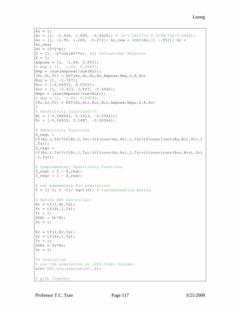
Luong
Professor T.C. Tsao Page 117 3/21/2008
Au = 1; Ac = [1, -2.446, 1.885, -0.4428]; % (z-1.081)*(z-0.9199)*(z-0.4453); Ao = [1, -1.95, 1.265, -0.273]; Ao_new = conv(Ao,[1 -.95]); Ao = Ao_new; w0 = 15*2*pi; D = [1, -2*cos(w0*Ts), 1]; %Sinusoidal Rejector E = 1; Ampnew = [1, -1.89, 0.893]; % Amp = [1, -1.89, 0.8959]; Bmp = (sum(Ampnew)/sum(Bu)); [Rt,St,Tt] = RST(Au,Ac,Bu,Bc,Ampnew,Bmp,D,E,Ao) Bur = [1, -1.707]; Bcr = [-0.06933, 0.0503]; Acr = [1, -2.453, 1.893, -0.4442]; Bmpr = (sum(Ampnew)/sum(Bur)); % Amp = [1, -1.89, 0.8959]; [Rr,Sr,Tr] = RST(Au,Acr,Bur,Bcr,Ampnew,Bmpr,D,E,Ao) % % sensitivity functions??? Bt = [-0.088641, 0.1913, -0.09421]; Br = [-0.06933, 0.1687, -0.08586]; % Sensitivity Functions S_regt = tf(Ac,1,Ts)*tf(Rt,1,Ts)/(tf(conv(Ac,Rt),1,Ts)+tf(conv(conv(Bu,Bc),St),1,Ts)); S_regr = tf(Ac,1,Ts)*tf(Rr,1,Ts)/(tf(conv(Ac,Rr),1,Ts)+tf(conv(conv(Bur,Bcr),Sr),1,Ts)); % Complementary Sensitivity Functions T_regt = 1 - S_regt; T_regr = 1 - S_regr; % set pamemeters for simulation; T = [1 1; 1 -1]/ sqrt(2); % transformation matrix % Define RST Controller; Rt = tf(1,Rt,Ts); St = tf(St,1,Ts); Tt = 1; SDRt = St*Rt; St = 1; Rr = tf(1,Rr,Ts); Sr = tf(Sr,1,Ts); Tr = 1; SDRr = Sr*Rr; Sr = 1; %% Simulation % run the simulation on 10th Order System; sim('RST_sin_simulation',1); % plot figures;
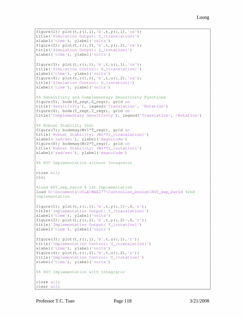
Luong
Professor T.C. Tsao Page 118 3/21/2008
figure(1); plot(t,r(:,1),'b',t,y(:,1),'rx'); title('Simulation Output: Y_{translation}') xlabel('time'), ylabel('volts') figure(2); plot(t,r(:,2),'b',t,y(:,2),'rx'); title('Simulation Output: Y_{rotation}') xlabel('time'), ylabel('volts') figure(3); plot(t,r(:,1),'b',t,u(:,1),'rx'); title('Simulation Control: U_{translation}') xlabel('time'), ylabel('volts') figure(4); plot(t,r(:,2),'b',t,u(:,2),'rx'); title('Simulation Control: U_{rotation}') xlabel('time'), ylabel('volts') %% Sensitivity and Complementary Sensitivity Functions figure(5), bode(S_regt,S_regr), grid on title('Sensitivity'), legend('Translation', 'Rotation') figure(6), bode(T_regt,T_regr), grid on title('Complementary Sensitivity'), legend('Translation', 'Rotation') %% Robust Stability Test figure(7); bodemag(Wr1*T_regt), grid on title('Robust Stability: (Wr*T)_{translation}') xlabel('rad/sec'), ylabel('magnitude') figure(8); bodemag(Wr2*T_regr), grid on title('Robust Stability: (Wr*T)_{rotation}') xlabel('rad/sec'), ylabel('magnitude') %% RST Implementation without Integrator close all; clc; %load RST_exp_David % 1st Implementation load G:\Documents\UCLA\MAE277\Controller_Design\RST_exp_David %2nd Implementation figure(1); plot(t,r(:,1),'b',t,y(:,1)-.6,'r'); title('Implementation Output: Y_{translation}') xlabel('time'), ylabel('volts') figure(2); plot(t,r(:,2),'b',t,y(:,2)-.6,'r'); title('Implementation Output: Y_{rotation}') xlabel('time'), ylabel('volts') figure(3); plot(t,r(:,1),'b',t,u(:,1),'r'); title('Implementation Control: U_{translation}') xlabel('time'), ylabel('volts') figure(4); plot(t,r(:,2),'b',t,u(:,2),'r'); title('Implementation Control: U_{rotation}') xlabel('time'), ylabel('volts') %% RST Implementation with Integrator close all; clear all;
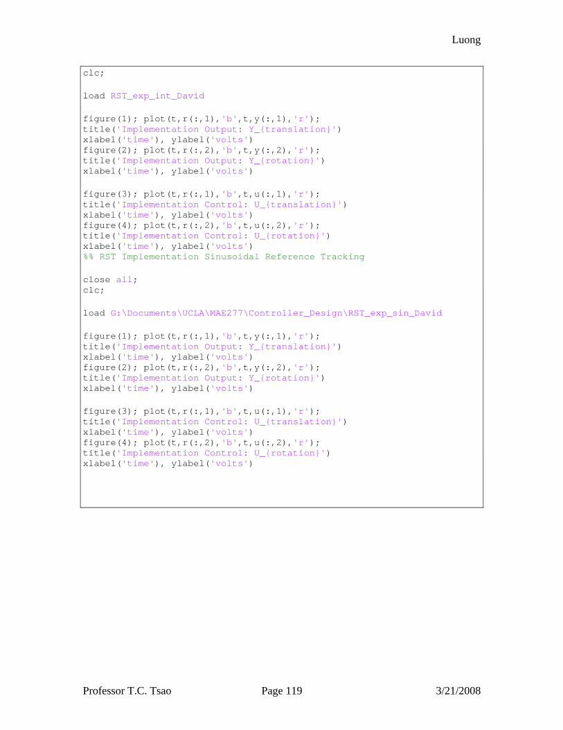
Luong
Professor T.C. Tsao Page 119 3/21/2008
clc; load RST_exp_int_David figure(1); plot(t,r(:,1),'b',t,y(:,1),'r'); title('Implementation Output: Y_{translation}') xlabel('time'), ylabel('volts') figure(2); plot(t,r(:,2),'b',t,y(:,2),'r'); title('Implementation Output: Y_{rotation}') xlabel('time'), ylabel('volts') figure(3); plot(t,r(:,1),'b',t,u(:,1),'r'); title('Implementation Control: U_{translation}') xlabel('time'), ylabel('volts') figure(4); plot(t,r(:,2),'b',t,u(:,2),'r'); title('Implementation Control: U_{rotation}') xlabel('time'), ylabel('volts') %% RST Implementation Sinusoidal Reference Tracking close all; clc; load G:\Documents\UCLA\MAE277\Controller_Design\RST_exp_sin_David figure(1); plot(t,r(:,1),'b',t,y(:,1),'r'); title('Implementation Output: Y_{translation}') xlabel('time'), ylabel('volts') figure(2); plot(t,r(:,2),'b',t,y(:,2),'r'); title('Implementation Output: Y_{rotation}') xlabel('time'), ylabel('volts') figure(3); plot(t,r(:,1),'b',t,u(:,1),'r'); title('Implementation Control: U_{translation}') xlabel('time'), ylabel('volts') figure(4); plot(t,r(:,2),'b',t,u(:,2),'r'); title('Implementation Control: U_{rotation}') xlabel('time'), ylabel('volts')
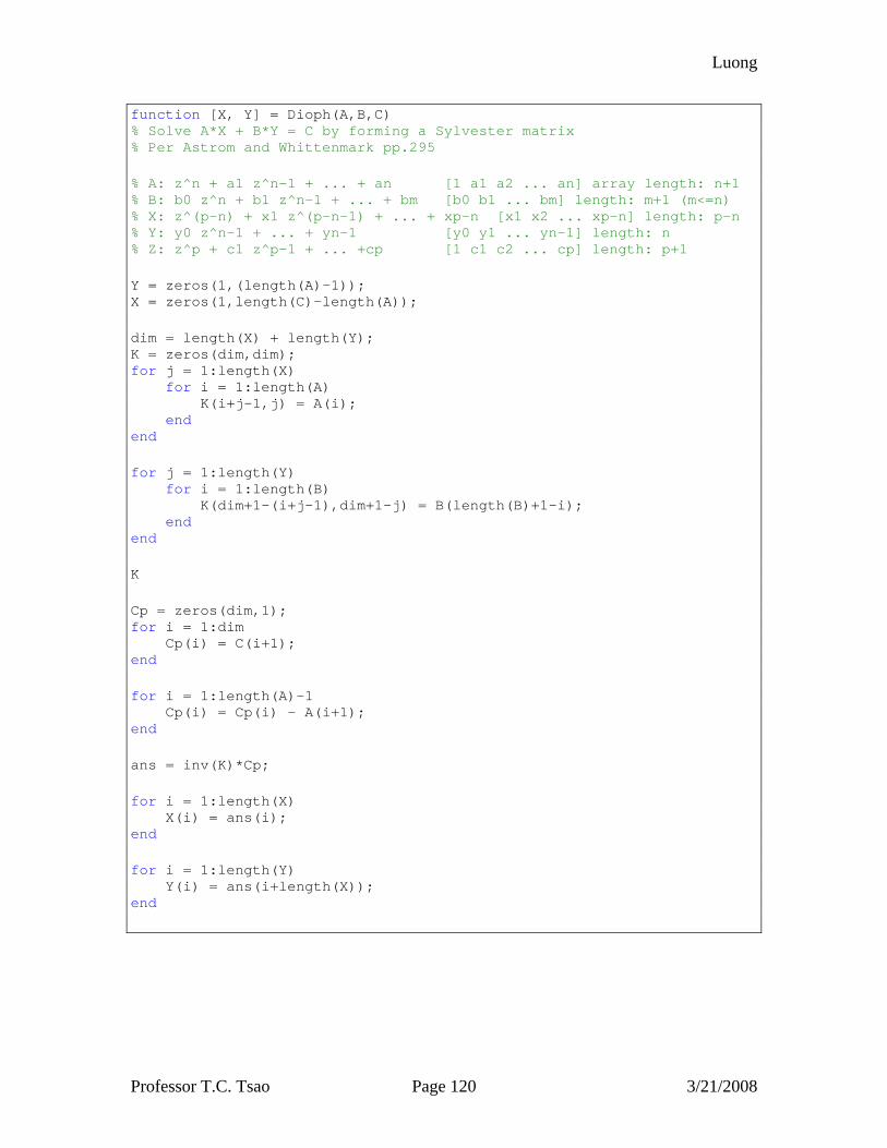
Luong
Professor T.C. Tsao Page 120 3/21/2008
function [X, Y] = Dioph(A,B,C) % Solve A*X + B*Y = C by forming a Sylvester matrix % Per Astrom and Whittenmark pp.295 % A: z^n + a1 z^n-1 + ... + an [1 a1 a2 ... an] array length: n+1 % B: b0 z^n + b1 z^n-1 + ... + bm [b0 b1 ... bm] length: m+1 (m<=n) % X: z^(p-n) + x1 z^(p-n-1) + ... + xp-n [x1 x2 ... xp-n] length: p-n % Y: y0 z^n-1 + ... + yn-1 [y0 y1 ... yn-1] length: n % Z: z^p + c1 z^p-1 + ... +cp [1 c1 c2 ... cp] length: p+1 Y = zeros(1,(length(A)-1)); X = zeros(1,length(C)-length(A)); dim = length(X) + length(Y); K = zeros(dim,dim); for j = 1:length(X) for i = 1:length(A) K(i+j-1,j) = A(i); end end for j = 1:length(Y) for i = 1:length(B) K(dim+1-(i+j-1),dim+1-j) = B(length(B)+1-i); end end K Cp = zeros(dim,1); for i = 1:dim Cp(i) = C(i+1); end for i = 1:length(A)-1 Cp(i) = Cp(i) - A(i+1); end ans = inv(K)*Cp; for i = 1:length(X) X(i) = ans(i); end for i = 1:length(Y) Y(i) = ans(i+length(X)); end
Luong
Professor T.C. Tsao Page 121 3/21/2008
function [R,S,T] = RST(Au,Ac,Bu,Bc,Amp,Bmp,D,E,Ao) % I/O model matching and pole placement % Solve Ac*D*Rpp + Bu*E*Spp = Ao*Amp by forming a Sylverster matrix % Per Astrom and Whittenmark pp.295 and Tsao's notes % use [X,Y] = Dioph(A,B,C) % plant: bp*bn/ap, (bp should be monic, bn should include unstable zeros?) % to obtain causal controllter, the following conditions must be satisfied: % Feedforward: deg(Amp) - deg(Bmp) >= deg(Ac) - deg(Bc) % Feedback: deg(Ao) >= 2*deg(A) + deg(D) + deg(E) - deg(Amp) - deg(Au) - % deg(Bc) - 1 A = conv(Ac,D); B = conv(Bu,E); C = conv(Ao,Amp); [Rpp,Spp] = Dioph(A,B,C); R = conv(Bc,conv(D,[1,Rpp])); S = conv(Au,conv(E,Spp)); T = conv(Bmp,Ao);
Luong
Professor T.C. Tsao Page 122 3/21/2008
% Example for Youla Parameterization and h2/hinf minimization; % % Some comments: % 1) for unstable plant, we must first find a stabilizing controller K0, % e.g, lead compensator. Then using closing the loop we get the % closed-loop system Ghat; % 2) the sensitivity function is fomulated as a function of the free % parameter Q, i.e., Wp*S = Wp - Ghat*Gp*Q = t1 - t2*Q; % 3) the goal is to minimize H_2 and H_inf norm of S; % % By Yigang Wang, 02/28/2007 close all; clear; clc; Fs = 5000; % sampling rate; h = 1/Fs; Ts = h; omega = logspace(0,5,300); % load the system models load sysGd11; load sysGd22; load sysWr; load G_y_10Order_96match; % plant model; sysGdz11 = c2d(sysGd11,h,'zoh'); sysGdz22 = c2d(sysGd22,h,'zoh'); % z-domain lead compensator; cdz11 = 3.5805*tf([1 -0.8394],[1 -0.4817],h); cdz22 = 3.0817*tf([1 -0.835],[1 -0.485],h); % closed-loop wr = wr_original * S wrz1 = minreal(wrz1/(1+sysGdz11*cdz11)); wrz2 = minreal(wrz2/(1+sysGdz22*cdz22)); % stable closed-loop Ghat; sysGhat11 = feedback(sysGdz11*cdz11,1); sysGhat22 = feedback(sysGdz22*cdz22,1); % Wpz : performance weight %%%% Modify this section for better performance %%%%%% wb1=2*pi*80; %cross-over frequency Ms=10^(5/20);%low frequency gain ep=10^(-10/20); %high frequency dcgain wp=makeweight(Ms,wb1,ep); wpz = c2d(wp,h,'tustin'); % calculate t1, t2; t1_11 = wpz; t2_11 = wpz*sysGhat11;
Luong
Professor T.C. Tsao Page 123 3/21/2008
t1_22 = wpz; t2_22 = wpz*sysGhat22; % H2 minimization; [q_h2_11 h2Gamma_11] = H2ModelMatching(t1_11,t2_11); [q_h2_22 h2Gamma_22] = H2ModelMatching(t1_22,t2_22); %% Sensitivity and Complementary Sensitivity % calculate sensitivity function; sen_h2_11 = minreal((t1_11-t2_11*q_h2_11)/wpz); sen_h2_22 = minreal((t1_22-t2_22*q_h2_22)/wpz); % another way to calculate sensitivity function; sen_h2_11n = 1-sysGhat11*q_h2_11; sen_h2_22n = 1-sysGhat22*q_h2_22; % calculate complementary sensitivity function; csen_h2_11n = sysGhat11*q_h2_11; csen_h2_22n = sysGhat22*q_h2_22; % performance S calculations; figure; subplot(211); bodemag(sen_h2_11); hold on; bodemag(sen_h2_11n); bodemag(1/wpz); grid on; legend('sensitivity function','sensitivity function','1/W_p',4); title('sensitivity function of sysGdz11'); subplot(212); bodemag(sen_h2_22); hold on; bodemag(sen_h2_22n); bodemag(1/wpz); grid on; legend('sensitivity function','sensitivity function','1/W_p',4); title('sensitivity function of sysGdz22'); % performance T calculations; figure; subplot(211); hold on; bodemag(csen_h2_11n); bodemag(1/wpz); grid on; legend('complementary sensitivity function','1/W_p',4); title('complementary sensitivity function of sysGdz11'); subplot(212); hold on; bodemag(csen_h2_22n); bodemag(1/wpz); grid on; legend('complementary sensitivity function','1/W_p',4); title('complementary sensitivity function of sysGdz22'); %% Robust Stability % robust stability TWR = Wr*T = TWR*(1-S) TWr1 = wrz1*(1-sen_h2_11); figure; subplot(211); bodemag(TWr1); grid on; axis([10 10^5 -50 5]); title('robust stability of sysGdz11: |TW_r|'); TWr2 = wrz2*(1-sen_h2_22); subplot(212); bodemag(TWr2); grid on; axis([10 10^5 -50 5]); title('robust stability of sysGdz22: |TW_r|'); %% High order plant simulation; % run the simulation; sim('MagBearing_x_axis_simulation',2); % plot figures; figure; plot(t,r(:,1),'b',t,y(:,1),'r'); title('Implementation Output: Y_{translation}')
Luong
Professor T.C. Tsao Page 124 3/21/2008
xlabel('time'), ylabel('volts') figure; plot(t,r(:,2),'b',t,y(:,2),'r'); title('Implementation Output: Y_{rotation}') xlabel('time'), ylabel('volts') figure; plot(t,r(:,1),'b',t,u(:,1),'r'); title('Implementation Control: U_{translation}') xlabel('time'), ylabel('volts') figure; plot(t,r(:,2),'b',t,u(:,2),'r'); title('Implementation Control: U_{rotation}') xlabel('time'), ylabel('volts') %% H2 Implementation close all; clear all; clc; load data_80_5_N10 figure(1); plot(t,r(:,1),'b',t,y(:,1),'r'); title('Implementation Output: Y_{translation}') xlabel('time'), ylabel('volts') figure(2); plot(t,r(:,2),'b',t,y(:,2),'r'); title('Implementation Output: Y_{rotation}') xlabel('time'), ylabel('volts') figure(3); plot(t,r(:,1),'b',t,u(:,1),'r'); title('Implementation Control: U_{translation}') xlabel('time'), ylabel('volts') figure(4); plot(t,r(:,2),'b',t,u(:,2),'r'); title('Implementation Control: U_{rotation}') xlabel('time'), ylabel('volts')
Luong
Professor T.C. Tsao Page 125 3/21/2008
function [Kz Gamma] = H2ModelMatching(Mz,Pz) % This function is used to solve H2-norm % minimization of Model Matching Problem, i.e. % min ||Mz-KzPz||_{2}; % % Written by Yigang Wang March 3, 2008 % % Note: % 1) Mz, Pz must be stable, but they can be any LTI form, i.e., ss,tf.. % 2) Currently, this function is only valid for SISO system; % Input parameters: % 1) Mz: reference model in z-domain; % 2) Pz: plant model in z-domain; % Output parameters: % 1) Kz: resulting controller in z-domain; % 2) Gamma: minimized Hinf norm; % converts everything into the continuous domain Ts = Mz.ts; M = d2c(Mz,'tustin'); P = d2c(Pz,'tustin'); % definining the interconnects in the system systemnames = 'M P'; inputvar = '[r; u]'; outputvar = '[M-P; r]'; input_to_M = '[r]'; input_to_P = '[u]'; T = sysic; % % runs the h2 synthesis toolkit % [K,CL,Gamma]=h2syn(T,1,1); % % % returns everything back into the discrete domain % Kz = c2d(K,Ts,'tustin'); % Gamma = norm(Mz-Pz*Kz,2); % runs the hinf synthesis toolkit [K,CL,Gamma]=hinfsyn(T,1,1); % returns everything back into the discrete domain Kz = c2d(K,Ts,'tustin'); Gamma = norm(Mz-Pz*Kz,inf);
Luong
Professor T.C. Tsao Page 126 3/21/2008
% MAE 277 Zero-Phase Error Tracking Controller % David Luong, Winter 2008 clear all close all load sysGd11 load sysGd22 load G_y_10Order_96match Ts = 1/5000 T = [1 1; 1 -1]/ sqrt(2) Gz11 = c2d(sysGd11,Ts,'zoh'); Gz22 = c2d(sysGd22,Ts,'zoh'); Cx1 = zpk([.9174],[.72],2.7163,Ts); Cx2 = Cx1; % step(1/(1+Gztrans*Cx1)) Ghat11 = minreal(Gz11*Cx1/(1+Gz11*Cx1)) figure(1),step(Ghat11) Ghat22 = minreal(Gz22*Cx2/(1+Gz22*Cx2)) figure(2),step(Ghat22) F11 = zeroPhase(Ghat11) F22 = zeroPhase(Ghat22) N1 = 2; sim('MagBearing_x_axis_simulation_ZeroPhase',.2) figure(3); plot(t,r(:,1),'b',t,y(:,1),'r'); title('Simulation Output: Y_{translation}') xlabel('time'), ylabel('volts') legend('reference','output') figure(4); plot(t,r(:,2),'b',t,y(:,2),'r'); title('Simulation Output: Y_{rotation}') xlabel('time'), ylabel('volts') legend('reference','output') figure(5); plot(t,r(:,1),'b',t,u(:,1),'r'); title('Simulation Control: U_{translation}') xlabel('time'), ylabel('volts') legend('reference','output') figure(6); plot(t,r(:,2),'b',t,u(:,2),'r'); title('Simulation Control: U_{rotation}') xlabel('time'), ylabel('volts') legend('reference','output') figure(7)
Luong
Professor T.C. Tsao Page 127 3/21/2008
plot(t,r(:,1)-y(:,1)) hold on plot(t,r(:,2)-y(:,2),'r') hold off title('Simulation Tracking Error'), xlabel('time'), ylabel('volts') legend('e_{translation}','e_{Rotation}') % Bode Plots of Compensated System figure(8) bode(F11*Ghat11) figure(9) bode(F22*Ghat22) %% Implementation clear all; clc; close all; load zeroPhaseHighFreq %Translation @ 100 Hz, Rotation @ 150 Hz %load zeroPhaseLowFreq %Translation @ 10 Hz, Rotation @ 20 Hz figure(1); plot(t,r(:,1),'b',t,y(:,1),'r'); title('Implementation Output: Y_{translation}') xlabel('time'), ylabel('volts') legend('reference','output') figure(2); plot(t,r(:,2),'b',t,y(:,2),'r'); title('Implementation Output: Y_{rotation}') xlabel('time'), ylabel('volts') legend('reference','output') figure(3); plot(t,r(:,1),'b',t,u(:,1),'r'); title('Implementation Control: U_{translation}') xlabel('time'), ylabel('volts') legend('reference','output') figure(4); plot(t,r(:,2),'b',t,u(:,2),'r'); title('Implementation Control: U_{rotation}') xlabel('time'), ylabel('volts') legend('reference','output') figure(5) plot(t,r(:,1)-y(:,1)) hold on plot(t,r(:,2)-y(:,2),'r') hold off title('Implementation Tracking Error'), xlabel('time'), ylabel('volts') legend('e_{translation}','e_{Rotation}')
Luong
Professor T.C. Tsao Page 128 3/21/2008
function xx = zeroPhase(Gsys) % this function returns a system transfer function % that when put in series with a stable system % Gsys will result in a linear phase system % note: only works on discrete siso systems [z,p,k,Ts] = zpkdata(Gsys,'v'); % find the cancelable and uncancelable parts ii = find(abs(z)<1); jj = find(abs(z)>=1); stableZ = z(ii); unstableZ = z(jj); % invert the invertable parts Ginv = zpk(p,stableZ,1/k,Ts); % take the Bstar transpose Bstar = fliplr(poly(unstableZ)); BstarTF = tf(Bstar,1,Ts); xx = BstarTF*Ginv/(sum(Bstar)^2); % make xx realizable [z,p,k] = zpkdata(xx,'v'); delay = max(length(z)-length(p),0); xx = xx*zpk([],zeros(1,delay),1,Ts);
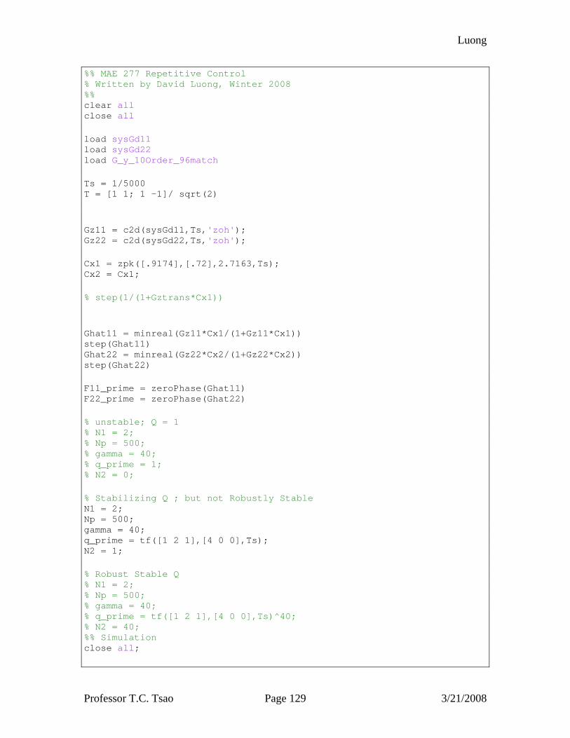
Luong
Professor T.C. Tsao Page 129 3/21/2008
%% MAE 277 Repetitive Control % Written by David Luong, Winter 2008 %% clear all close all load sysGd11 load sysGd22 load G_y_10Order_96match Ts = 1/5000 T = [1 1; 1 -1]/ sqrt(2) Gz11 = c2d(sysGd11,Ts,'zoh'); Gz22 = c2d(sysGd22,Ts,'zoh'); Cx1 = zpk([.9174],[.72],2.7163,Ts); Cx2 = Cx1; % step(1/(1+Gztrans*Cx1)) Ghat11 = minreal(Gz11*Cx1/(1+Gz11*Cx1)) step(Ghat11) Ghat22 = minreal(Gz22*Cx2/(1+Gz22*Cx2)) step(Ghat22) F11_prime = zeroPhase(Ghat11) F22_prime = zeroPhase(Ghat22) % unstable; Q = 1 % N1 = 2; % Np = 500; % gamma = 40; % q_prime = 1; % N2 = 0; % Stabilizing Q ; but not Robustly Stable N1 = 2; Np = 500; gamma = 40; q_prime = tf([1 2 1],[4 0 0],Ts); N2 = 1; % Robust Stable Q % N1 = 2; % Np = 500; % gamma = 40; % q_prime = tf([1 2 1],[4 0 0],Ts)^40; % N2 = 40; %% Simulation close all;
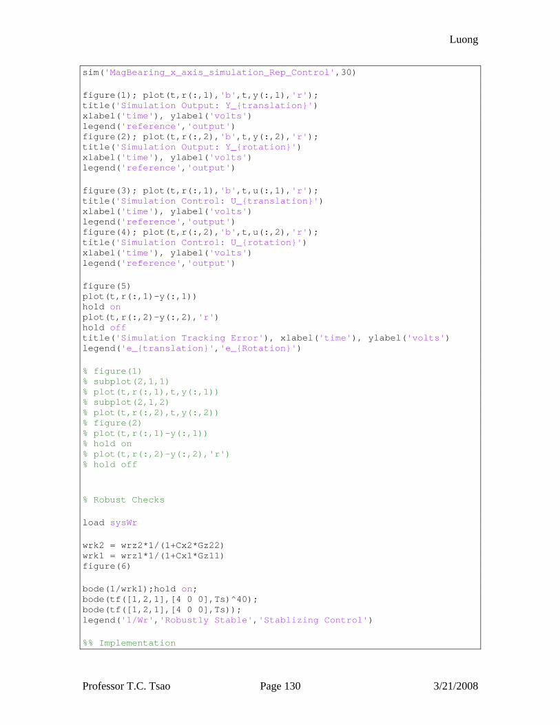
Luong
Professor T.C. Tsao Page 130 3/21/2008
sim('MagBearing_x_axis_simulation_Rep_Control',30) figure(1); plot(t,r(:,1),'b',t,y(:,1),'r'); title('Simulation Output: Y_{translation}') xlabel('time'), ylabel('volts') legend('reference','output') figure(2); plot(t,r(:,2),'b',t,y(:,2),'r'); title('Simulation Output: Y_{rotation}') xlabel('time'), ylabel('volts') legend('reference','output') figure(3); plot(t,r(:,1),'b',t,u(:,1),'r'); title('Simulation Control: U_{translation}') xlabel('time'), ylabel('volts') legend('reference','output') figure(4); plot(t,r(:,2),'b',t,u(:,2),'r'); title('Simulation Control: U_{rotation}') xlabel('time'), ylabel('volts') legend('reference','output') figure(5) plot(t,r(:,1)-y(:,1)) hold on plot(t,r(:,2)-y(:,2),'r') hold off title('Simulation Tracking Error'), xlabel('time'), ylabel('volts') legend('e_{translation}','e_{Rotation}') % figure(1) % subplot(2,1,1) % plot(t,r(:,1),t,y(:,1)) % subplot(2,1,2) % plot(t,r(:,2),t,y(:,2)) % figure(2) % plot(t,r(:,1)-y(:,1)) % hold on % plot(t,r(:,2)-y(:,2),'r') % hold off % Robust Checks load sysWr wrk2 = wrz2*1/(1+Cx2*Gz22) wrk1 = wrz1*1/(1+Cx1*Gz11) figure(6) bode(1/wrk1);hold on; bode(tf([1,2,1],[4 0 0],Ts)^40); bode(tf([1,2,1],[4 0 0],Ts)); legend('1/Wr','Robustly Stable','Stablizing Control') %% Implementation
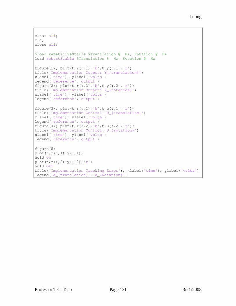
Luong
Professor T.C. Tsao Page 131 3/21/2008
clear all; clc; close all; %load repetitiveStable %Translation @ Hz, Rotation @ Hz load robustStable %Translation @ Hz, Rotation @ Hz figure(1); plot(t,r(:,1),'b',t,y(:,1),'r'); title('Implementation Output: Y_{translation}') xlabel('time'), ylabel('volts') legend('reference','output') figure(2); plot(t,r(:,2),'b',t,y(:,2),'r'); title('Implementation Output: Y_{rotation}') xlabel('time'), ylabel('volts') legend('reference','output') figure(3); plot(t,r(:,1),'b',t,u(:,1),'r'); title('Implementation Control: U_{translation}') xlabel('time'), ylabel('volts') legend('reference','output') figure(4); plot(t,r(:,2),'b',t,u(:,2),'r'); title('Implementation Control: U_{rotation}') xlabel('time'), ylabel('volts') legend('reference','output') figure(5) plot(t,r(:,1)-y(:,1)) hold on plot(t,r(:,2)-y(:,2),'r') hold off title('Implementation Tracking Error'), xlabel('time'), ylabel('volts') legend('e_{translation}','e_{Rotation}')
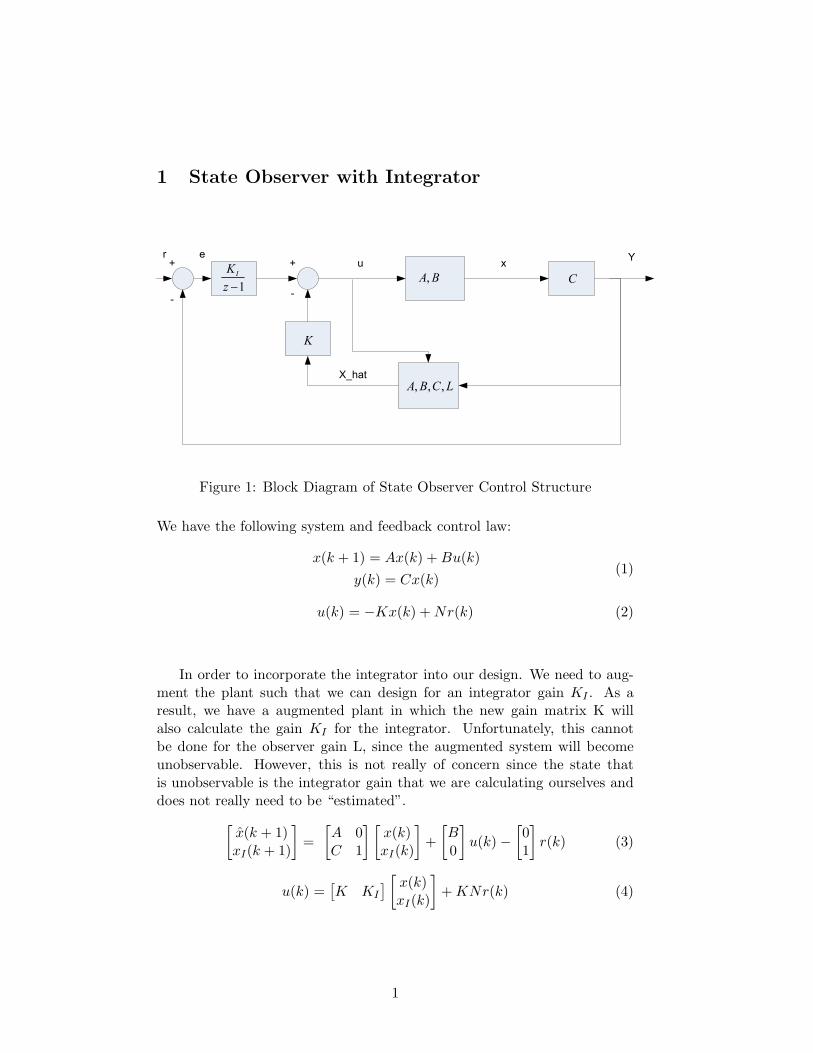
1 State Observer with Integrator
1
IK
z ,A B C
, , ,A B C L
K
uer Y
x
X_hat
--
++
Figure 1: Block Diagram of State Observer Control Structure
We have the following system and feedback control law:
x(k + 1) = Ax(k) + Bu(k)
y(k) = Cx(k)(1)
u(k) = −Kx(k) + Nr(k) (2)
In order to incorporate the integrator into our design. We need to aug-ment the plant such that we can design for an integrator gain KI . As aresult, we have a augmented plant in which the new gain matrix K willalso calculate the gain KI for the integrator. Unfortunately, this cannotbe done for the observer gain L, since the augmented system will becomeunobservable. However, this is not really of concern since the state thatis unobservable is the integrator gain that we are calculating ourselves anddoes not really need to be “estimated”.
[
x(k + 1)xI(k + 1)
]
=
[
A 0C 1
] [
x(k)xI(k)
]
+
[
B
0
]
u(k) −
[
01
]
r(k) (3)
u(k) =[
K KI
]
[
x(k)xI(k)
]
+ KNr(k) (4)
1
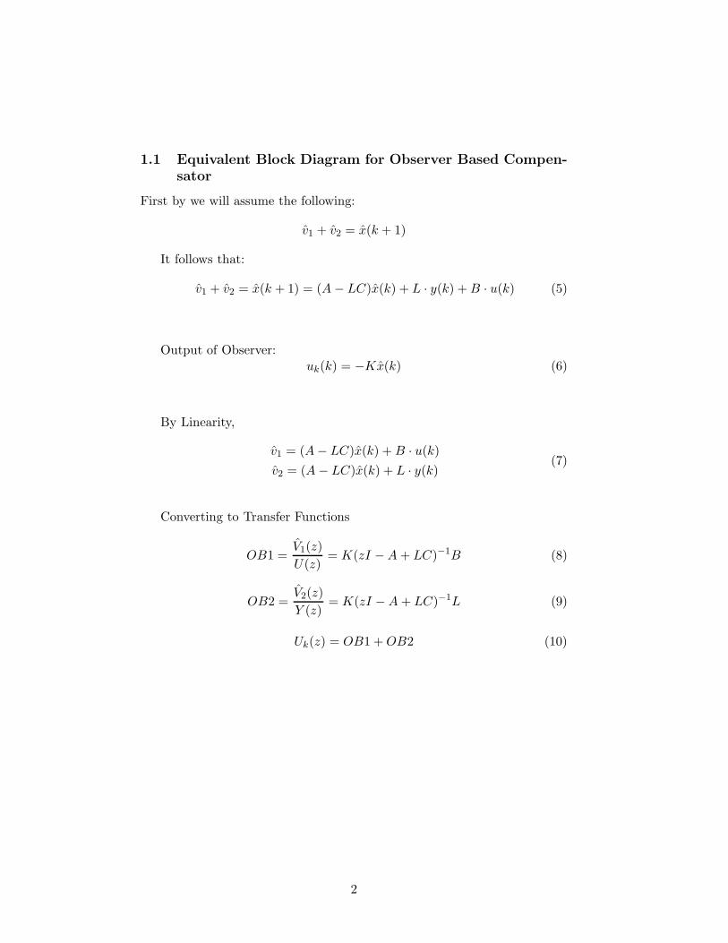
1.1 Equivalent Block Diagram for Observer Based Compen-
sator
First by we will assume the following:
v1 + v2 = x(k + 1)
It follows that:
v1 + v2 = x(k + 1) = (A − LC)x(k) + L · y(k) + B · u(k) (5)
Output of Observer:uk(k) = −Kx(k) (6)
By Linearity,
v1 = (A − LC)x(k) + B · u(k)
v2 = (A − LC)x(k) + L · y(k)(7)
Converting to Transfer Functions
OB1 =V1(z)
U(z)= K(zI − A + LC)−1B (8)
OB2 =V2(z)
Y (z)= K(zI − A + LC)−1L (9)
Uk(z) = OB1 + OB2 (10)
2
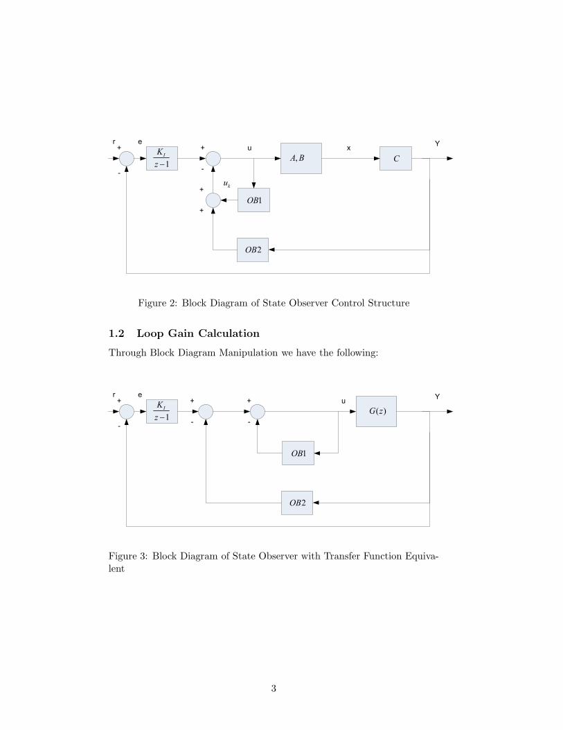
1
IK
z ,A B C
uer Y
x
--
++
1OB
+
+
2OB
ku
Figure 2: Block Diagram of State Observer Control Structure
1.2 Loop Gain Calculation
Through Block Diagram Manipulation we have the following:
1
IK
z ( )G z
uer Y
--
++
1OB
-
+
2OB
Figure 3: Block Diagram of State Observer with Transfer Function Equiva-lent
3
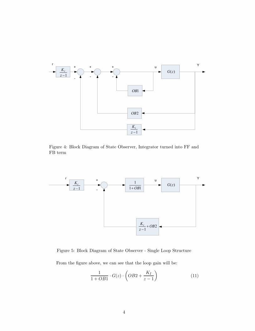
( )G z
ur Y
--
++
1OB
-
+
2OB
1
IK
z
1
IK
z
Figure 4: Block Diagram of State Observer, Integrator turned into FF andFB term
( )G z
ur Y
-
+
1
IK
z
1
1 1OB!
21
IK
OBz
!
Figure 5: Block Diagram of State Observer - Single Loop Structure
From the figure above, we can see that the loop gain will be:
1
1 + OB1· G(z) ·
(
OB2 +KI
z − 1
)
(11)
4
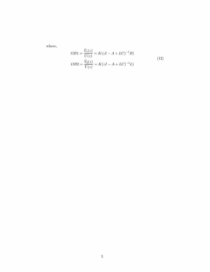
where,
OB1 =V1(z)
U(z)= K(zI − A + LC)−1B)
OB2 =V2(z)
Y (z)= K(zI − A + LC)−1L)
(12)
5


