57
Advanced Empirical Economics I Mario Larch Chair of Empirical Economics University of Bayreuth [email protected] WS 2016/17 Mario Larch 1 / 354 AEE I, WS 2016/17

Advanced Empirical Economics I
Mario Larch
Chair of Empirical EconomicsUniversity of Bayreuth
WS 2016/17
Mario Larch 1 / 354 AEE I, WS 2016/17

Introduction
Table of content I1 Introduction
2 Linear modelsIdentificationConsistencyLimit distributionAsymptotic distributionHeteroskedasticity-robust standard errors for OLS
Weighted least squares (WLS)Generalized least-squares (GLS) and Feasible GLSWeighted Least Squares (WLS)
Model misspecificationInconsistency of OLSFunctional form misspecificationEndogeneityOmitted variablesPseudo-true valuesParameter heterogeneity
Instrumental variablesMario Larch 2 / 354 AEE I, WS 2016/17

Introduction
Table of content IIInconsistency of OLSInstrumentsInstrumental variables estimatorWald estimatorIV estimation for multiple regressionTwo-stage least squaresAn exampleWeak instrumentsInconsistency of IV estimatorsLow precision and finite-sample bias
3 Maximum likelihoodPoisson regressionClassificationAn m-estimatorLikelihood functionMaximum likelihood estimator
Regularity conditions
Mario Larch 3 / 354 AEE I, WS 2016/17

Introduction
Table of content IIIInformation matrix equalityDistribution of the ML estimator
Quasi-maximum likelihoodMarginal effectsAn example
4 Generalized method of moments (GMM)ExamplesMethod of moments estimator (MM)Generalized method of moments estimator (GMM)
Distribution of GMM estimatorOptimal weighting matrixOptimal moment conditions
Linear IVNon-linear IV
Mario Larch 4 / 354 AEE I, WS 2016/17

Introduction
Introduction
• Question for Students: Background and expectations.• Focus: Methods and microeconometrics.• But also: Applications.• Organization:
• Start: Monday, 05.12.2016.• End: Tuesday, 07.02.2017.• No lectures between 21.12.2016-08.01.2017.• Hence: 6 lectures before Christmas, 10 lectures after
Christmas (16 in total).• Exam: Will be announced in the elearning.
Mario Larch 5 / 354 AEE I, WS 2016/17

Introduction
Introduction
• This course provides a comprehensive treatment of mainlymicroeconometric methods, allowing to analyseindividual-level data on the economic behaviour ofindividuals or firms using regression methods applied tocross-section and panel data.
• The linear regression model will be discussed, but basicknowledge is assumed. The course will use matrixalgebra. A short refresher will be given if wished.
• However, orientation toward the practitioner.
Mario Larch 6 / 354 AEE I, WS 2016/17

Introduction
Introduction
• Main Reference: Cameron, A. Colin and Pravin K. Trivedi(2005), Microeconometrics - Methods and Applications,Cambridge University Press (price at Amazon about Euro100).
• http://cameron.econ.ucdavis.edu/mmabook/mma.html• Compagnion: Cameron, A. Colin and Pravin K. Trivedi
(2010), Microeconometrics using STATA, STATACorp LP.(price at Amazon about Euro 80).
Mario Larch 7 / 354 AEE I, WS 2016/17

Introduction
Introduction“Methodology, like sex, is better demonstrated than discussed,though often better anticipated than experienced” (Leamer,1983, Let’s Take the Con Out of Econometrics, AmericanEconomic Review 73(1), p. 40)
Tutorials (two):• Group 1: Monday (16-18h) and Tuesday (18-20h), (start
05.12.).• Group 2: Monday (18-20h) and Tuesday (16-18h), (start
05.12.).• Rooms: S 56 (RW I) and 2.01 (AI).• Both held by: Joschka Wanner.• Software: Scilab (http://www.scilab.org/).
Mario Larch 8 / 354 AEE I, WS 2016/17

Introduction
Introduction
Main empirical courses at our chair:• Bachelor level:
• Empirical Economics I: Introduction, data problems, OLS,Gauss-Markov-Theorem, heteroskedasticity,autocorrelation, correlation versus causation.
• Empirical Economics II: Stochastic processes, panel dataestimators (SUR, diff-in-diff, fixed effects, random effects),time series econometrics (ARMA, (P)ACF, forecasting).
• Master level:• Advanced Empirical Economics I: Estimation methods
(linear and non-linear least squares, MLE, GMM),applications.
• Advanced Empirical Economics II: “Topic”-courses (e.g.,time series econometrics, program evaluation methods,spatial econometrics,...).
Mario Larch 9 / 354 AEE I, WS 2016/17

Introduction
Introduction
Are you familiar with the following concepts?• Consistency.• Bias.• Limit distribution.• Asymptotic distribution.• Omitted variable bias.• Information matrix.• Quasi-Maximum likelihood.• Central limit theorem.• Law of large numbers.
Mario Larch 10 / 354 AEE I, WS 2016/17

Introduction
Introduction
Occurring themes and problems:• Data are often discrete or censored, in which case
non-linear methods such as logit, probit, and Tobit modelsare used.
• Distributional assumptions for such data become criticallyimportant.
• Economic studies often aim to determine causation ratherthan merely measure correlation.
• Microeconomic data are typically collected usingcross-section and panel surveys, censuses, or socialexperiments.
Mario Larch 11 / 354 AEE I, WS 2016/17

Introduction
Introduction
Occurring themes and problems:• It is not unusual that two or more complications occur
simultaneously.• Large data-sets.• Microeconomic/Behavioural foundation, allowing to employ
a structural approach.
Mario Larch 12 / 354 AEE I, WS 2016/17

Linear models
Table of content I1 Introduction
2 Linear modelsIdentificationConsistencyLimit distributionAsymptotic distributionHeteroskedasticity-robust standard errors for OLS
Weighted least squares (WLS)Generalized least-squares (GLS) and Feasible GLSWeighted Least Squares (WLS)
Model misspecificationInconsistency of OLSFunctional form misspecificationEndogeneityOmitted variablesPseudo-true valuesParameter heterogeneity
Instrumental variablesMario Larch 13 / 354 AEE I, WS 2016/17

Linear models
Table of content IIInconsistency of OLSInstrumentsInstrumental variables estimatorWald estimatorIV estimation for multiple regressionTwo-stage least squaresAn exampleWeak instrumentsInconsistency of IV estimatorsLow precision and finite-sample bias
3 Maximum likelihoodPoisson regressionClassificationAn m-estimatorLikelihood functionMaximum likelihood estimator
Regularity conditions
Mario Larch 14 / 354 AEE I, WS 2016/17
Linear models
Table of content IIIInformation matrix equalityDistribution of the ML estimator
Quasi-maximum likelihoodMarginal effectsAn example
4 Generalized method of moments (GMM)ExamplesMethod of moments estimator (MM)Generalized method of moments estimator (GMM)
Distribution of GMM estimatorOptimal weighting matrixOptimal moment conditions
Linear IVNon-linear IV
Mario Larch 15 / 354 AEE I, WS 2016/17

Linear models
Linear models
• In modern microeconometrics the term regression refers toa bewildering range of procedures for studying therelationship between an outcome variable y and a set ofregressors x.
• The simplest example of regression is the OLS estimator inthe linear regression model.
• After first defining the model and estimator, a quite detailedpresentation of the asymptotic distribution of the OLSestimator is given.
• The exposition presumes previous exposure to a moreintroductory treatment.
• The model assumptions made here permit stochasticregressors and heteroskedastic errors and accommodatedata that are obtained by exogenous stratified sampling.
Mario Larch 16 / 354 AEE I, WS 2016/17

Linear models
Notation and conventions
Vectors are defined as column vectors and represented usinglower-case bold. For example, for linear regression theregressor vector x is a K × 1 column vector with j th entry xj andthe parameter vector β is a K × 1 column vector with j th entryβj , so
x =(K × 1)
x1...
xK
and β =(K × 1)
β1...βK
.
Mario Larch 17 / 354 AEE I, WS 2016/17
Linear models
Notation and conventions
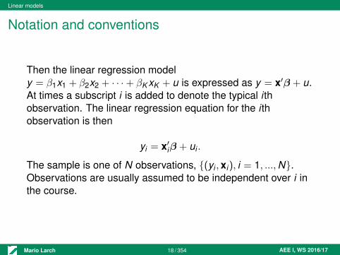
Then the linear regression modely = β1x1 + β2x2 + · · ·+ βK xK + u is expressed as y = x′β + u.At times a subscript i is added to denote the typical i thobservation. The linear regression equation for the i thobservation is then
yi = x′iβ + ui .
The sample is one of N observations, (yi ,xi), i = 1, ...,N.Observations are usually assumed to be independent over i inthe course.
Mario Larch 18 / 354 AEE I, WS 2016/17
Linear models
Notation and conventions
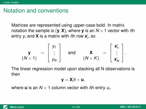
Matrices are represented using upper-case bold. In matrixnotation the sample is (y,X), where y is an N × 1 vector with i thentry yi and X is a matrix with i th row x′i , so
y =(N × 1)
y1...
yN
and X =(N × K )
x′1...
x′N
.The linear regression model upon stacking all N observations isthen
y = Xβ + u,
where u is an N × 1 column vector with i th entry ui .
Mario Larch 19 / 354 AEE I, WS 2016/17

Linear models
Linear regression model
• In a standard cross-section regression model with Nobservations on a scalar dependent variable and severalregressors, the data are specified as (y,X), where ydenotes observations on the dependent variable and Xdenotes a matrix of explanatory variables.
• The general regression model with additive errors is writtenin vector notation as
y = E [y|X] + u, (1)
where E [y|X] denotes the conditional expectation of therandom variable y given X, and u denotes a vector ofunobserved random errors or disturbances.
Mario Larch 20 / 354 AEE I, WS 2016/17
Linear models
Linear regression model
• The right-hand side of this equation decomposes y into twocomponents, one that is deterministic given the regressorsand one that is attributed to random variation or noise.
• We think of E [y|X] as a conditional prediction function thatyields the average value, or more formally the expectedvalue, of y given X.
• A linear regression model is obtained when E [y|X] isspecified to be a linear function of X.
Mario Larch 21 / 354 AEE I, WS 2016/17

Linear models
Linear regression model
• y is referred to as the dependent variable or endogenousvariable whose variation we wish to study in terms ofvariation in x and u.
• u is referred to as the error term or disturbance term in thepopulation.
• x is referred to as regressors or predictors or covariates.• Note, the sample equivalent of equation y = E [y|X] + u is
y = Xβ + u, where u is the residual vector and β is thevector of the OLS estimates.
Mario Larch 22 / 354 AEE I, WS 2016/17

Linear models
OLS estimator• The OLS estimator is defined to be the estimator that
minimizes the sum of squared errors
N∑i=1
u2i = u′u =
(y− Xβ
)′ (y− Xβ
). (2)
In other words:
minˆβ
S(β) =(
y− Xβ)′ (
y− Xβ). (3)
• Expanding S(β) gives:
minˆβ
S(β) = y′y− β′X′y− y′Xβ + β
′X′Xβ (4)
= y′y− 2y′Xβ + β′X′Xβ. (5)
Mario Larch 23 / 354 AEE I, WS 2016/17

Linear models
OLS estimator
• The necessary condition for a minimum is given by the firstderivative with respect to β set equal to 0:
∂S(β)
∂β= −2X′y + 2X′Xβ = 0. (6)
• Solving for β yields the OLS estimator,
βOLS =(X′X
)−1 X′y. (7)
Mario Larch 24 / 354 AEE I, WS 2016/17
Linear models
OLS estimator
• If X′X is of less than full rank, the inverse can be replacedby a generalized inverse.
• Then OLS estimation still yields the optimal linear predictorof y given x if squared error loss is used.
• But many different linear combinations of x will yield thisoptimal predictor.
Mario Larch 25 / 354 AEE I, WS 2016/17

Linear models
Identification
• The OLS estimator can always be computed, provided thatX′X is non-singular.
• The more interesting issue is what βOLS tells us about thedata.
• We focus on the ability of the OLS estimator to permitidentification of the conditional mean E [y|X].
Mario Larch 26 / 354 AEE I, WS 2016/17
Linear models
Identification
For the linear model the parameter β is identified if1 E [y|X] = Xβ.2 Xβ(1) = Xβ(2) if and only if β(1) = β(2) (implies that X′X is
non-singular), i.e. that βOLS is the unique solution ofmin ˆβ
S(β).
Mario Larch 27 / 354 AEE I, WS 2016/17

Linear models
Consistency
• The properties of an estimator depend on the process thatactually generated the data, the data generating process(dgp).
• We assume the dgp is y = Xβ + u.• Then:
βOLS =(X′X
)−1 X′y
=(X′X
)−1 X′ (Xβ + u)
=(X′X
)−1 X′Xβ +(X′X
)−1 X′u
= β +(X′X
)−1 X′u.
Mario Larch 28 / 354 AEE I, WS 2016/17

Linear models
Excursus: Asymptotic theory
• Good, more accessible treatment: van der Vaart, A. W.(1998), Asymptotic Statistics, Cambridge University Press.
• Thorough discussion: White, H. (2000), Asymptotic Theoryfor Econometricians, Academic Press.
• Thorough discussion with focus on dynamic models:Prucha, I., B. Pötscher (1997), Dynamic NonlinearEconometric Models: Asymptotic Theory, Springer, Berlin.
Mario Larch 29 / 354 AEE I, WS 2016/17
Linear models
Excursus: Asymptotic theory
• In this excursus we consider the behaviour of a sequenceof random variables bN as N →∞.
• For estimation theory it is sufficient to focus on twoaspects:
1 Convergence in probability of bN to a limit b, a constant orrandom variable that is very close to bN in a probabilisticsense defined in the following.
2 If the limit b is a random variable, we consider the limitdistribution.
• Estimators are usually functions of averages or sums.Then it is easiest to derive limiting results by invokingresults on the behaviour of averages, notably laws of largenumbers and central limit theorems.
Mario Larch 30 / 354 AEE I, WS 2016/17
Linear models
Excursus: Asymptotic theoryConvergence in probability• Because of the intrinsic randomness of a sample we can
never be certain that a sequence bN , such as an estimatorθ (often denoted θN to make clear that it is a sequence),will be within a given small distance of its limit, even if thesample is infinitely large.
• However, we can be almost certain.• Different ways of expressing this near certainty correspond
to different types of convergence of a sequence of randomvariables to a limit.
• The one most used in econometrics is convergence inprobability.
• Others are: Mean-square convergence, almost sureconvergence.
Mario Larch 31 / 354 AEE I, WS 2016/17

Linear models
Excursus: Asymptotic theory
Convergence in probability• Recall that a sequence of non-stochastic real numbersaN converges to a if, for any ε > 0, there existsN∗ = N∗(ε) such that, for all N > N∗:
|aN − a| < ε. (8)
• Example: If aN = 2 + 3/N, then the limit is a = 2 since|aN − a| = |2 + 3/N − 2| = |3/N| < ε for all N > N∗ = 3/ε.
Mario Larch 32 / 354 AEE I, WS 2016/17
Linear models
Excursus: Asymptotic theory
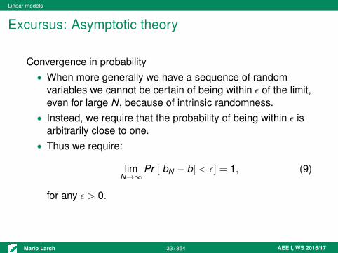
Convergence in probability• When more generally we have a sequence of random
variables we cannot be certain of being within ε of the limit,even for large N, because of intrinsic randomness.
• Instead, we require that the probability of being within ε isarbitrarily close to one.
• Thus we require:
limN→∞
Pr [|bN − b| < ε] = 1, (9)
for any ε > 0.
Mario Larch 33 / 354 AEE I, WS 2016/17

Linear models
Excursus: Asymptotic theory
Convergence in probability• A formal definition is the following:
Definition: Convergence in probability
A sequence of random variables bN converges in probabilityto b if, for any ε > 0 and δ > 0, there exists N∗ = N∗(ε, δ) suchthat, for all N > N∗, Pr [|bN − b| < ε] > 1− δ.
• We write plim bN = b, where plim is shorthand forprobability limit, or bN
p→ b.
Mario Larch 34 / 354 AEE I, WS 2016/17

Linear models
Excursus: Asymptotic theory
Consistency• When the sequence bN is a sequence of parameter
estimates θ, we have a large sample analogue ofunbiasedness, consistency.
• A formal definition is the following:
Definition: Consistency
An estimator θ is consistent for θ0 if plim θ = θ0.
Mario Larch 35 / 354 AEE I, WS 2016/17

Linear models
Excursus: Asymptotic theoryConsistency• Note that unbiasedness need not imply consistency.• Unbiasedness states only that the expected value of θ isθ0, and it permits variability around θ0 that need notdisappear as the sample size goes to infinity.
• Also, a consistent estimator need not be unbiased.• For example, adding 1/N to an unbiased and consistent
estimator produces a new estimator that is biased but stillconsistent.
• Although the sequence of vector random variables bNmay converge to a random variable b, in manyeconometric applications bN converges to a constant.
• For example, we hope that an estimator of a parameter willconverge in probability to the parameter itself.
Mario Larch 36 / 354 AEE I, WS 2016/17

Linear models
Excursus: Asymptotic theoryConsistencySlutsky’s TheoremLet bN be a finite-dimensional vector of random variables, andg(·) be a real-valued function continuous at a constant vectorpoint b. Then
bNp→ b⇒ g(bN)
p→ g(b).
• Slutsky’s Theorem is one of the major reasons for theprevalence of asymptotic results versus finite-sampleresults in econometrics.
• It states a very convenient property that does not hold forexpectations.
• For example, plim(bN) = plim(b1N ,b2N) = (b1,b2) impliesplim(b1Nb2N) = b1b2, whereas E [b1Nb2N ] generally differsfrom E [b1]E [b2].
Mario Larch 37 / 354 AEE I, WS 2016/17

Linear models
Excursus: Asymptotic theory
Laws of large numbers• Laws of large numbers are theorems for convergence in
probability in the special case where the sequence bN isa sample average, that is, bN = XN , where
XN =1N
N∑i=1
Xi . (10)
• Note that Xi here is general notation for a random variable,and in the regression context it does not necessarilydenote the regressor variables.
Mario Larch 38 / 354 AEE I, WS 2016/17

Linear models
Excursus: Asymptotic theory
Laws of large numbers• A law of large numbers provides a much easier way to
establish the probability limit of a sequence bN than thealternatives of brute-force use of the (ε, δ) definition.
Definition: Law of large numbers
A (weak) law of large numbers (LLN) specifies conditions on theindividual terms Xi in XN under which (XN − E [XN ])
p→ 0.
Mario Larch 39 / 354 AEE I, WS 2016/17

Linear models
Excursus: Asymptotic theory
Laws of large numbers• It can be helpful to think of a LLN as establishing that XN
goes to its expected value, even though strictly speaking itimplies the weaker condition that XN goes to the limit of itsexpected value, since the above condition implies that:
plim XN = lim E [XN ]. (11)
• If the Xi have common mean µ, then this simplifies toplim XN = µ.
Mario Larch 40 / 354 AEE I, WS 2016/17
Linear models
Consistency
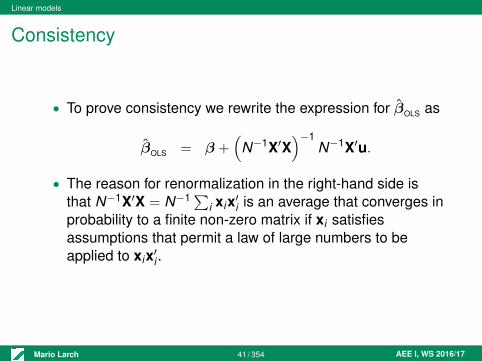
• To prove consistency we rewrite the expression for βOLS as
βOLS = β +(
N−1X′X)−1
N−1X′u.
• The reason for renormalization in the right-hand side isthat N−1X′X = N−1∑
i xix′i is an average that converges inprobability to a finite non-zero matrix if xi satisfiesassumptions that permit a law of large numbers to beapplied to xix′i .
Mario Larch 41 / 354 AEE I, WS 2016/17

Linear models
Consistency
• Then we may write
plim βOLS = β +(
plim N−1X′X)−1 (
plim N−1X′u),
using Slutsky’s Theorem (Theorem A.3).• The OLS estimator is consistent for β (i.e., plim βOLS = β) if
plim N−1X′u = 0.
• If a law of large numbers can be applied to the averageN−1X′u = N−1∑
i xiui then a necessary condition for theprevious expression to hold is that E [xiui ] = 0.
Mario Larch 42 / 354 AEE I, WS 2016/17

Linear models
Excursus: Asymptotic theory
Convergence in distribution• Given consistency, the estimator θ has a degenerate
distribution that collapses on θ0 as N →∞.• We need to magnify or rescale θ to obtain a random
variable that has non-degenerate distribution as N →∞.• Often the appropriate scale factor is
√N, in which case we
consider the behaviour of the sequence of randomvariables bN =
√N(θ − θ0
).
Mario Larch 43 / 354 AEE I, WS 2016/17

Linear models
Excursus: Asymptotic theory
Convergence in distribution• In general, the Nth random variable in the sequence bN
has an extremely complicated cumulative distributionfunction (cdf) FN .
• Like any other function FN , this may have a limit functionwhere convergence is in the usual mathematical sense.
Definition: Convergence in distribution
A sequence of random variables bN is said to converge in dis-tribution to a random variable b if limN→∞ FN = F , at every con-tinuity point of F , where FN is the distribution of bN , F is thedistribution of b, and convergence is in the usual mathematicalsense.
Mario Larch 44 / 354 AEE I, WS 2016/17

Linear models
Excursus: Asymptotic theoryConvergence in distribution
• We write bNd→ b, and we call F the limit distribution of
bN.• Convergence in probability implies convergence in
distribution; that is, bNp→ b implies bN
d→ b.• In general, the converse is not true.• For example, let bN = XN , the Nth realization of
X ∼ N [µ, σ2].
• Then bNd→ N [µ, σ2], but (bN − b) has variance that does
not disappear as N →∞, so bN does not converge inprobability to b.
• In the special case where b is a constant, however, bNd→ b
implies bNp→ b.
• In this case the limit distribution is degenerate, with all itsmass at b.
Mario Larch 45 / 354 AEE I, WS 2016/17

Linear models
Excursus: Asymptotic theory
Central limit theorems• Central limit theorems are theorems on convergence in
distribution when the sequence bN is a sample average.• A central limit theorem provides a simpler way to obtain the
limit distribution of a sequence bN than the alternativessuch as brute-force use of convergence in distribution.
• From a law of large numbers, the sample average has adegenerate distribution as it converges to a constant,lim E [XN ].
• So we scale(XN − E [XN ]
)by its standard deviation to
construct a random variable with unit variance that mayconverge to a non-degenerate distribution.
Mario Larch 46 / 354 AEE I, WS 2016/17
Linear models
Excursus: Asymptotic theory
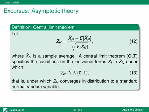
Definition: Central limit theoremLet
ZN =XN − E [XN ]√
V [XN ], (12)
where XN is a sample average. A central limit theorem (CLT)specifies the conditions on the individual terms Xi in XN underwhich
ZNd→ N (0,1), (13)
that is, under which ZN converges in distribution to a standardnormal random variable.
Mario Larch 47 / 354 AEE I, WS 2016/17
Linear models
Excursus: Asymptotic theory
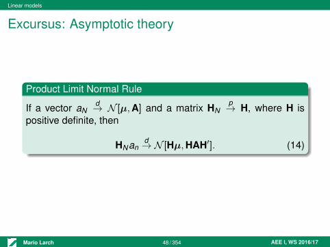
Product Limit Normal Rule
If a vector aNd→ N [µ,A] and a matrix HN
p→ H, where H ispositive definite, then
HNand→ N [Hµ,HAH′]. (14)
Mario Larch 48 / 354 AEE I, WS 2016/17

Linear models
Limit distribution
• Given consistency, the limit distribution of βOLS isdegenerate with all the mass at β.
• To obtain the limit distribution we multiply βOLS by√
N, asthis rescaling leads to a random variable that understandard cross-section assumptions has non-zero yet finitevariance asymptotically.
• Then we may write:
√N(βOLS − β
)=(
N−1X′X)−1
N−1/2X′u. (15)
Mario Larch 49 / 354 AEE I, WS 2016/17

Linear models
Limit distribution
• The proof of consistency assumed that plim N−1X′X existsand is finite and non-zero.
• We assume that a central limit theorem can be applied toN−1/2X′u to yield a multivariate normal limit distributionwith finite, non-singular covariance matrix.
• Applying the product rule for limit normal distributions(Theorem A.17), i.e., HN =
(N−1X′X
)−1 andaN = N−1/2X′u implies that the product in the right-handside of (15) has a limit normal distribution.
Mario Larch 50 / 354 AEE I, WS 2016/17

Linear models
Limit distribution
This leads to the following proposition, which permitsregressors to be stochastic and does not restrict model errorsto be homoskedastic.Distribution of OLS estimatorMake the following assumptions:
1 The dgp is y = Xβ + u.2 Data are independent over i with E [u|X] = 0 and
E [uu′|X] = Ω = Diag[σ2i ].
3 The matrix X has full rank so that Xβ(1) = Xβ(2) iffβ(1) = β(2).
Mario Larch 51 / 354 AEE I, WS 2016/17

Linear models
Distribution of OLS estimatorMake the following assumptions:
4 The K × K matrix
MXX = plim N−1X′X = plim1N
N∑i=1
xix′i = lim1N
N∑i=1
E [xix′i ],
exists and is finite non-singular.5 The K × 1 vector
N−1/2X′u = N−1/2∑Ni=1 xiui
d→ N [0,MxΩx], where
MxΩx = plim N−1X′uu′X = plim1N
N∑i=1
u2i xix′i
= lim1N
N∑i=1
E [u2i xix′i ].
Mario Larch 52 / 354 AEE I, WS 2016/17

Linear models
Limit distribution
Hence, the OLS estimator βOLS is consistent for β and
√N(βOLS − β)
d→ N [0,M−1xx MxΩxM−1
xx ]. (16)
Mario Larch 53 / 354 AEE I, WS 2016/17

Linear models
Asymptotic distribution
• So far we have stated the limit distribution of√N(βOLS − β), a rescaling of βOLS.
• Many practitioners prefer to see asymptotic results writtendirectly in terms of the distribution of βOLS.
• This distribution is called an asymptotic distribution.• The asymptotic distribution is interpreted as being
applicable in large samples, meaning samples largeenough for the limit distribution to be a good approximationbut not so large that βOLS
p→ β as then its asymptoticdistribution would be degenerate.
Mario Larch 54 / 354 AEE I, WS 2016/17

Linear models
Asymptotic distribution
• The asymptotic distribution is obtained from (16) bydivision by N−1/2 and addition of β.
• This yields the asymptotic distribution
βOLSa∼ N [β,N−1M−1
xx MxΩxM−1xx ], (17)
where the symbol a∼ means is “asymptotically distributedas.”
• The variance matrix in (17) is called the asymptoticvariance matrix of βOLS and is denoted V [βOLS].
Mario Larch 55 / 354 AEE I, WS 2016/17

Linear models
Asymptotic distribution
• Even simpler notation drops the limits and expectations inthe definitions of Mxx and MxΩx and the asymptoticdistribution is denoted
βOLSa∼ N [β, (X′X)−1(X′ΩX)(X′X)−1], (18)
and V [βOLS] is defined to be the variance matrix in (18).
Mario Larch 56 / 354 AEE I, WS 2016/17

Linear models
Asymptotic distribution
• For implementation, the matrices Mxx and MxΩx arereplaced by consistent estimates Mxx and MxΩx.
• Then the estimated asymptotic variance matrix of βOLS is
V [βOLS] = N−1M−1xx MxΩxM−1
xx . (19)
• This estimate is called a sandwich estimate, with MxΩxsandwiched between M−1
xx and M−1xx .
Mario Larch 57 / 354 AEE I, WS 2016/17


