75
ADVANCED FIN OF REIN SCHOOL OF NITE ELEMENT MODELLI NFORCED CONCRETE TURNED IN: 16/06/2017 F ENGINEERING AND SCIENCE ING
ADVANCED FINITE ELEM
OF REINFORCED CONCRE
SCHOOL OF ENGINEERIN
ADVANCED FINITE ELEMENT MODELLING
OF REINFORCED CONCRETE
TURNED IN: 16/06/2017
SCHOOL OF ENGINEERING AND SCIENCE
ENT MODELLING

Title:
Advanced finite element modelling of reinforced
concrete
Project period: FEB. 2017
Report page numbers: 70
Appendix page numbers:
University: Aalborg University
Student:
Advanced finite element modelling of reinforced Nicolás Toro Martinez
2017 – JUN. 2017 Supervisor:
70 Johan Clausen
Appendix page numbers: 12 Turned in: 16th
Aalborg University
Nicolás Toro Martinez
June 2017

4
PREFACE
This report presents the Master’s thesis written by Nicolás Toro Martinez in agreement
with Aalborg University concerning the Msc in structural and civil engineering. This
report was written during the period from 1-02-2017 to 16-06-2017. Great gratitude is
extended on behalf of the author to my supervisor, Johan Clausen.
All the equations, tables and figures are referenced. Equations are named by the
chapter which they are shown, commentary text is written below figures and tables.

5
TABLE OF CONTENTS
1 INTRODUCTION 8
1.1 AIM AND MOTIVATION 8
1.2 OUTLINE OF THE REPORT 9
2 MATERIALS 10
2.1 CONCRETE 10
2.2 STEEL 11
3 YIELD CRITERIA 13
4 RESULTS VERIFICATION 14
4.1 ANALLYTICAL CALCULATIONS 14
4.2 NUMERICAL CALCULATIONS 16
4.3 COMPARISON 19
PART I-DOUBLY REINFORCED CONCRETE BEAM 21
1 INTRODUCTION 22
2 PLAIN CONCRETE BEAM 23
2.1 ANALLYTICAL CALCULATIONS 23
2.2 NUMERICAL CALCULATIONS 27
2.3 COMPARISON 28
3 DOUBLY REINFORCED CONCRETE BEAM 30
3.1 ANALLYTICAL CALCULATIONS 30
3.2 NUMERICAL CALCULATIONS 36
3.3 COMPARISON 39
6
PART II-REINFORCED CONCRETE COLUMN 44
1 INTRODUCTION 45
2 PLAIN CONCRETE COLUMN 46
2.1 ANALLYTICAL CALCULATIONS 46
2.2 NUMERICAL CALCULATIONS 48
2.3 COMPARISON 49
3 REINFORCED CONCRETE COLUMN 51
3.1 ANALLYTICAL CALCULATIONS 51
3.2 NUMERICAL CALCULATIONS 52
3.3 COMPARISON 54
PART III-CONCLUSION 58
1 CONCLUSIONS 59
REFERENCES 60
APPENDIX A: YIELD CRITERIA THEORY 62
1.1 MOHR COULOMB (MC) 62
1.2 CONCRETE DAMAGE PLASTICITY (CDP) 64
1.3 VON MISES (VM) 66
APPENDIX B: RESULTS VERIFICATION 69
APPENDIX C: PLAIN CONCRETE BEAM 70
APPENDIX D: REINFORCED CONCRETE BEAM 71
APPENDIX E: REINFORCED CONCRETE COLUMN 75

7

8
1 INTRODUCTION
In this chapter, the aim of this report will be presented as well as the
delimitations established.
1.1 AIM AND MOTIVATION
Nowadays, the use of reinforced concrete is considerably extended for all
types of structures. Therefore, it is important to understand the behaviour of
this composite material formed of concrete and steel. By doing this,
calculations will be more accurate which will help to save high amount and
material and thus, reduce the cost of constructions.
As an example, the Three Gorges hydropower Dam constructed in China is
shown in the Figure 1 in which millions of tons were needed for its
construction.
Figure 1. Three Gorges Dam, China (Wikimedia.org, 2004)

9
In this report, it will be analysed specifically the mechanical behaviour of
concrete and steel when they are bond, i.e., when they are merged together
to form reinforced concrete. To fulfil such purpose, 2 different structural
elements will be assessed: doubly reinforced concrete beam subjected to
bending and reinforced concrete column undergoing axial load.
Modelling of reinforced concrete is complex and the interface between the
concrete matrix and steel reinforcement must be accounted for. Non-linear
behaviour of reinforce concrete structures will be assessed numerically.
Thereafter, the numerical results will be compared to analytical calculations
leading to final results which will be presented and discussed.
1.2 OUTLINE OF THE REPORT
The use of shear reinforcement (stirrups) will out of the scope of this report
and the yield criteria used will be Von Misses, Mohr Coulomb and Concrete
Damage plasticity.
10
2 MATERIALS
In this chapter, the properties of the composite material to be used
(reinforced concrete) will be stated as well as its elastic and plastic behaviour.
2.1 CONCRETE
Concrete or also known as plain concrete stating that is not mixed with any
other material, is a highly worldwide used material for construction purposes.
Concrete is a composite material itself since it is composed of water, cement
and aggregates. Its high use in construction is due to the following
advantages presented below:
› It is considered highly economical compared to other materials such as
steel.
› Its resistance to fire which gives considerable safety particularly to
buildings.
› For architectural purposes, concrete is nearly always the most suitable
option since a wide range of shapes can be created.
› The availability of the materials to create concrete (aggregates, water
and cement) is high at any location.
› Its mechanical properties are well known to withstand loads, particularly
its resistance to compression.
As all materials, concrete has a main weakness; its low resistance to tension
(usually 10% of its compressive resistance). However, this problem is well
solved by the addition of steel bars to concrete to form reinforced concrete.
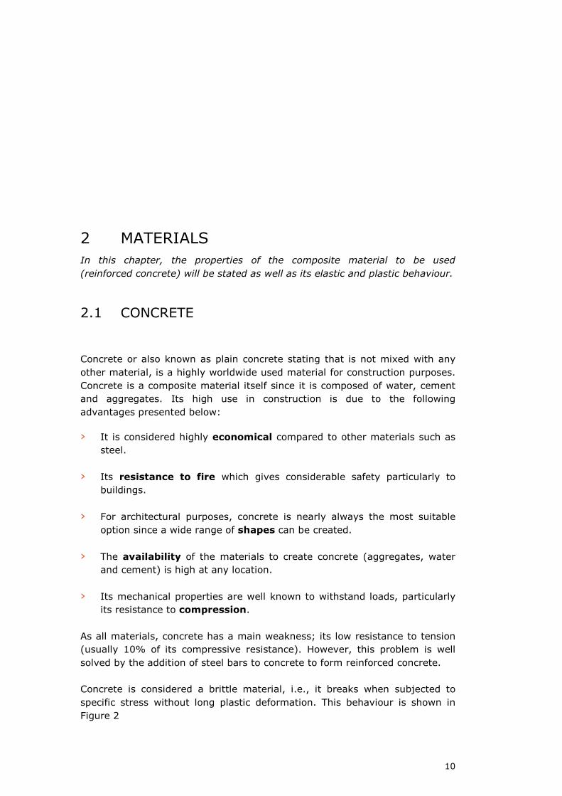
Concrete is considered a brittle material, i.e., it breaks when subjected to
specific stress without long plastic deformation. This behaviour is shown in
Figure 2
11
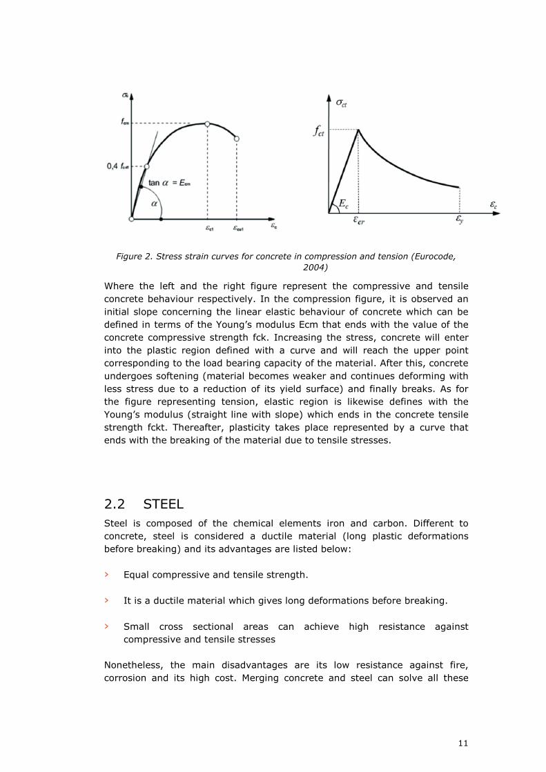
Figure 2. Stress strain curves for concrete in compression and tension (Eurocode,
2004)
Where the left and the right figure represent the compressive and tensile
concrete behaviour respectively. In the compression figure, it is observed an
initial slope concerning the linear elastic behaviour of concrete which can be
defined in terms of the Young’s modulus Ecm that ends with the value of the
concrete compressive strength fck. Increasing the stress, concrete will enter
into the plastic region defined with a curve and will reach the upper point
corresponding to the load bearing capacity of the material. After this, concrete
undergoes softening (material becomes weaker and continues deforming with
less stress due to a reduction of its yield surface) and finally breaks. As for
the figure representing tension, elastic region is likewise defines with the
Young’s modulus (straight line with slope) which ends in the concrete tensile
strength fckt. Thereafter, plasticity takes place represented by a curve that
ends with the breaking of the material due to tensile stresses.
2.2 STEEL
Steel is composed of the chemical elements iron and carbon. Different to
concrete, steel is considered a ductile material (long plastic deformations
before breaking) and its advantages are listed below:
› Equal compressive and tensile strength.
› It is a ductile material which gives long deformations before breaking.
› Small cross sectional areas can achieve high resistance against
compressive and tensile stresses
Nonetheless, the main disadvantages are its low resistance against fire,
corrosion and its high cost. Merging concrete and steel can solve all these
12
drawbacks mentioned before and that is why reinforced concrete is the most
suitable solution.
In Figure 3 can be seen the stress strain relationship for steel valid for
compression and tension.
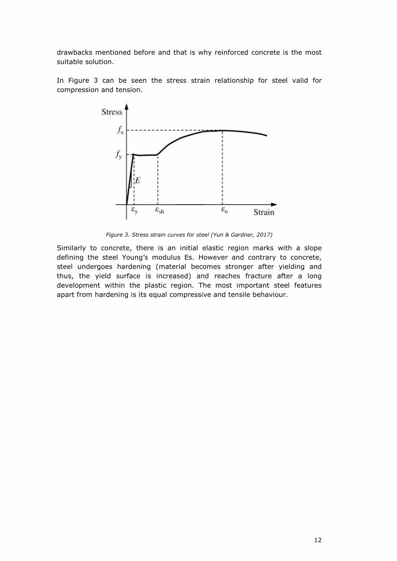
Figure 3. Stress strain curves for steel (Yun & Gardner, 2017)
Similarly to concrete, there is an initial elastic region marks with a slope
defining the steel Young’s modulus Es. However and contrary to concrete,
steel undergoes hardening (material becomes stronger after yielding and
thus, the yield surface is increased) and reaches fracture after a long
development within the plastic region. The most important steel features
apart from hardening is its equal compressive and tensile behaviour.
13
3 YIELD CRITERIA
In this chapter, the different yield criteria used for the numerical calculations
will be described. These are fundamental to represent material plastic
behaviour and to verify which criterion fits best with the non linear behaviour
of reinforced concrete. Theory of yield criteria can be found in APPENDIX A.

14
4 RESULTS VERIFICATION
In this chapter, a verification of the accuracy of modelling reinforced concrete
will be performed. A reinforced concrete sample will be tested analytical and
numerically and the results will be compared to check their reliability.
4.1 ANALLYTICAL CALCULATIONS
A reinforced concrete sample will be tested under axial loading. The supports
are assumed to be set in the neutral axis. There will be a pinned support
(ux=0, uy=0) in one end and a roller support (uy=0) in the other end. Its
geometry and static system are shown in Figure 12 and sample data is shown
in Table 1
Figure 4. Sample cross section and static system
Length, l[mm]
Width, b [mm]
Height, h [mm]
Diameter, Ø [mm]
Force, F [N]
100 20 20 10 104
Table 1. Sample data
As it can be seen on Figure 12, an axial load will be applied to the sample and
thus, it will undergo an horizontal displacement ux. To calculate such

15
displacement, Hook’s law must be applied since the materials will be modelled
only with elastic response. This is shown in Equation (4.1)
� = �� (4.1)
Where F is the force, k is the stiffness and x is the displacement. In this case,
the notation of x will be ux since it will be analyzed its horizontal
displacement. Hence. The resultant equation will be F=kux. It is necessary
also to consider that the 2 materials of the sample are acting in parallel and
not in series Both approaches are shown in Figure 5
Figure 5. Parallel and series springs based on Hook's law (Wikipedia, 2017)
The approach concerning this sample is the parallel springs. The equivalent
axial stiffness of the system keq can be found in Equation
��� = �� + � (4.2)
Where kc is the concrete axial stiffness
�� = � �� (4.3)
Being Ac the concrete cross sectional area, Ec the concrete Young’s modulus
and l the length of the sample. And the steel axial stiffness is defined as
� = � (4.4)
Being As the steel cross sectional area and Es the steel Young’s modulus.
In Table 2 is presented all the material parameters to take into account for
this calculation
Ac
[mm2]
As
[mm2]
Ec
[MPa]
Es
[MPa]
321.46 78.54 31500 2.1x10⁵
Table 2. Sample material parameters
16
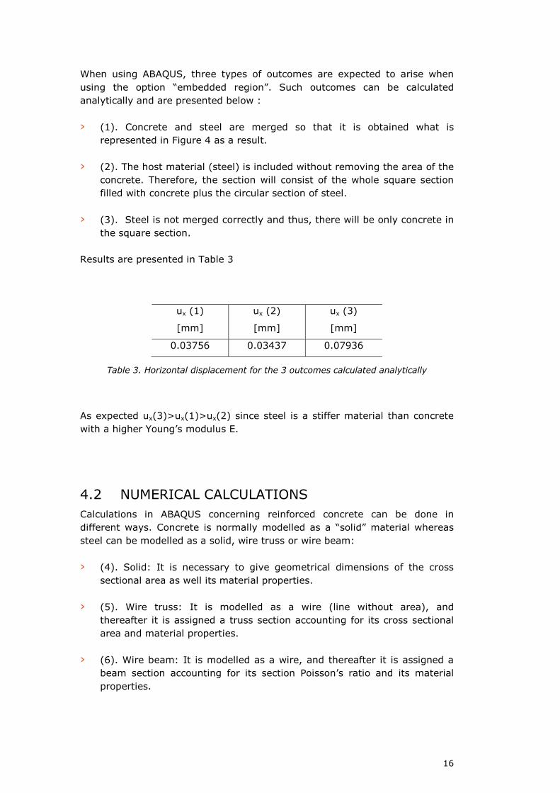
When using ABAQUS, three types of outcomes are expected to arise when
using the option “embedded region”. Such outcomes can be calculated
analytically and are presented below :
› (1). Concrete and steel are merged so that it is obtained what is
represented in Figure 4 as a result.
› (2). The host material (steel) is included without removing the area of the
concrete. Therefore, the section will consist of the whole square section
filled with concrete plus the circular section of steel.
› (3). Steel is not merged correctly and thus, there will be only concrete in
the square section.
Results are presented in Table 3
ux (1)
[mm]
ux (2)
[mm]
ux (3)
[mm]
0.03756 0.03437 0.07936
Table 3. Horizontal displacement for the 3 outcomes calculated analytically
As expected ux(3)>ux(1)>ux(2) since steel is a stiffer material than concrete
with a higher Young’s modulus E.
4.2 NUMERICAL CALCULATIONS
Calculations in ABAQUS concerning reinforced concrete can be done in
different ways. Concrete is normally modelled as a “solid” material whereas
steel can be modelled as a solid, wire truss or wire beam:
› (4). Solid: It is necessary to give geometrical dimensions of the cross
sectional area as well its material properties.
› (5). Wire truss: It is modelled as a wire (line without area), and
thereafter it is assigned a truss section accounting for its cross sectional
area and material properties.
› (6). Wire beam: It is modelled as a wire, and thereafter it is assigned a
beam section accounting for its section Poisson’s ratio and its material
properties.
17
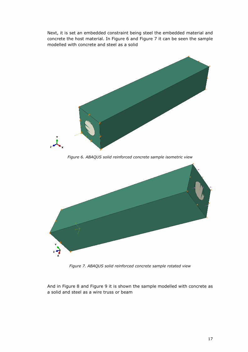
Next, it is set an embedded constraint being steel the embedded material and
concrete the host material. In Figure 6 and Figure 7 it can be seen the sample
modelled with concrete and steel as a solid
Figure 6. ABAQUS solid reinforced concrete sample isometric view
Figure 7. ABAQUS solid reinforced concrete sample rotated view
And in Figure 8 and Figure 9 it is shown the sample modelled with concrete as
a solid and steel as a wire truss or beam

18
Figure 8. ABAQUS wire truss/beam reinforced concrete sample isometric view
Figure 9. ABAQUS wire truss/beam reinforced concrete sample rotated view

19
To define the boundary conditions, it is important to account for the principal
axis x,y and z. The horizontal displacement ux calculated analytically will
correspond to uz in numerical calculations since it is seen in Figure 6 that the
axis in ABAQUS in z and not x. Therefore, and in order to avoid confusion,
ux=uz when presenting numerical results.
Since in ABAQUS it is used a 3d model, the axial force used analytically (2d) f=104 has to be divided by the cross sectional area of the sample (Asample=20x20=400mm2) and consequently, it is obtained the pressure P=f/Asample=104N/400mm2=25N/mm2.
The input material parameters introduced in ABAQUS are presented in Table 4
as well as the load.
νc
[-]
νs
[-]
Ec
[MPa]
Es
[MPa]
Pressure, P
[MPa]
0.18 0.30 31500 2.1x10⁵ 25
Table 4. ABAQUS Input parameters for concrete and steel
Where νc is the concrete Poisson’s ratio and νs is the steel Poisson’s ratio.
The numerical results are presented in Table 5
ux (4)
[mm]
ux (5)
[mm]
ux (6)
[mm]
0.03905 0.04303 0.04697
Table 5. Horizontal displacement for the 3 outcomes calculated numerically
4.3 COMPARISON
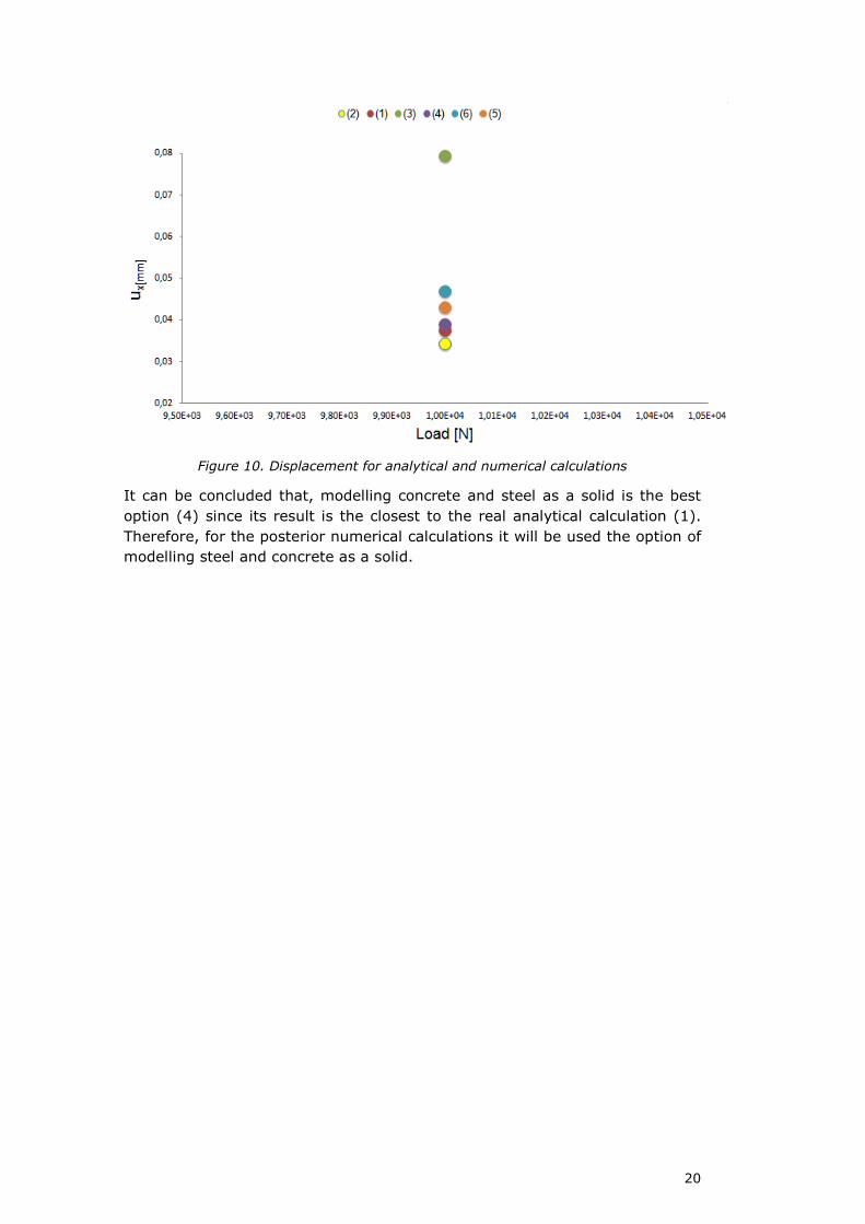
Results obtained analytically and numerically are compared and shown in Table 6 and in Figure 10
ux (1)
[mm]
ux (2)
[mm]
ux (3)
[mm]
ux (4)
[mm]
ux (5)
[mm]
ux (6)
[mm]
0.03756 0.03437 0.07936 0.03905 0.04303 0.04697
Table 6. Displacements for analytical and numerical calculations
20
Figure 10. Displacement for analytical and numerical calculations
It can be concluded that, modelling concrete and steel as a solid is the best
option (4) since its result is the closest to the real analytical calculation (1).
Therefore, for the posterior numerical calculations it will be used the option of
modelling steel and concrete as a solid.
21
PART I
DOUBLY REINFORCED CONCRETE
BEAM
22
1 INTRODUCTION
In this part, a non-linear analysis of a plain and a doubly reinforced concrete
beam will performed. Analytical and numerical solutions will be used and
conclusions will be drawn.
23
2 PLAIN CONCRETE BEAM
In this chapter, a plain concrete beam will be tested with analytical and
numerical solutions. The beam will be modelled as a elasto-plastic material
with the yield criterion von Misses and its non-linear behaviour will be
analyzed.
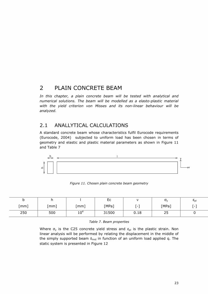
2.1 ANALLYTICAL CALCULATIONS
A standard concrete beam whose characteristics fulfil Eurocode requirements
(Eurocode, 2004) subjected to uniform load has been chosen in terms of
geometry and elastic and plastic material parameters as shown in Figure 11
and Table 7
Figure 11. Chosen plain concrete beam geometry
b
[mm]
h
[mm]
l
[mm]
Ec
[MPa]
ν
[-]
σy
[MPa]
εpl
[-]
250 500 104 31500 0.18 25 0
Table 7. Beam properties
Where σy is the C25 concrete yield stress and εpl is the plastic strain. Non
linear analysis will be performed by relating the displacement in the middle of
the simply supported beam ẟmid in function of an uniform load applied q. The
static system is presented in Figure 12
24
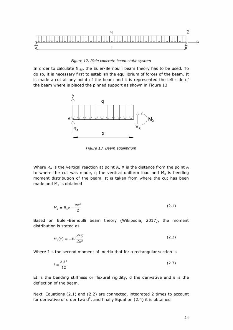
Figure 12. Plain concrete beam static system
In order to calculate ẟmid, the Euler-Bernoulli beam theory has to be used. To
do so, it is necessary first to establish the equilibrium of forces of the beam. It
is made a cut at any point of the beam and it is represented the left side of
the beam where is placed the pinned support as shown in Figure 13
Figure 13. Beam equilibrium
Where RA is the vertical reaction at point A, X is the distance from the point A
to where the cut was made, q the vertical uniform load and Mx is bending
moment distribution of the beam. It is taken from where the cut has been
made and Mx is obtained
�� = ��� − ���2 (2.1)
Based on Euler-Bernoulli beam theory (Wikipedia, 2017), the moment
distribution is stated as
����� = −�� ������ (2.2)
Where I is the second moment of inertia that for a rectangular section is
� = � ℎ�12 (2.3)
EI is the bending stiffness or flexural rigidity, d the derivative and ẟ is the
deflection of the beam.
Next, Equations (2.1) and (2.2) are connected, integrated 2 times to account
for derivative of order two d2, and finally Equation (2.4) it is obtained
25
��� = ���24 �2 − �� + !"� + !� (2.4)
Where C1 and C2 are the integral constants. These can be obtained by setting
two boundary conditions:
› 1. Vertical displacement is ẟ=0 for x=l
› 2. Vertical displacement is ẟ=0 for x=0
Applying the correspondent boundary conditions and replacing C1 and C2 in
Equation (2.4) , Equation (2.5) is obtained
�#$% = − 5� '384�� (2.5)
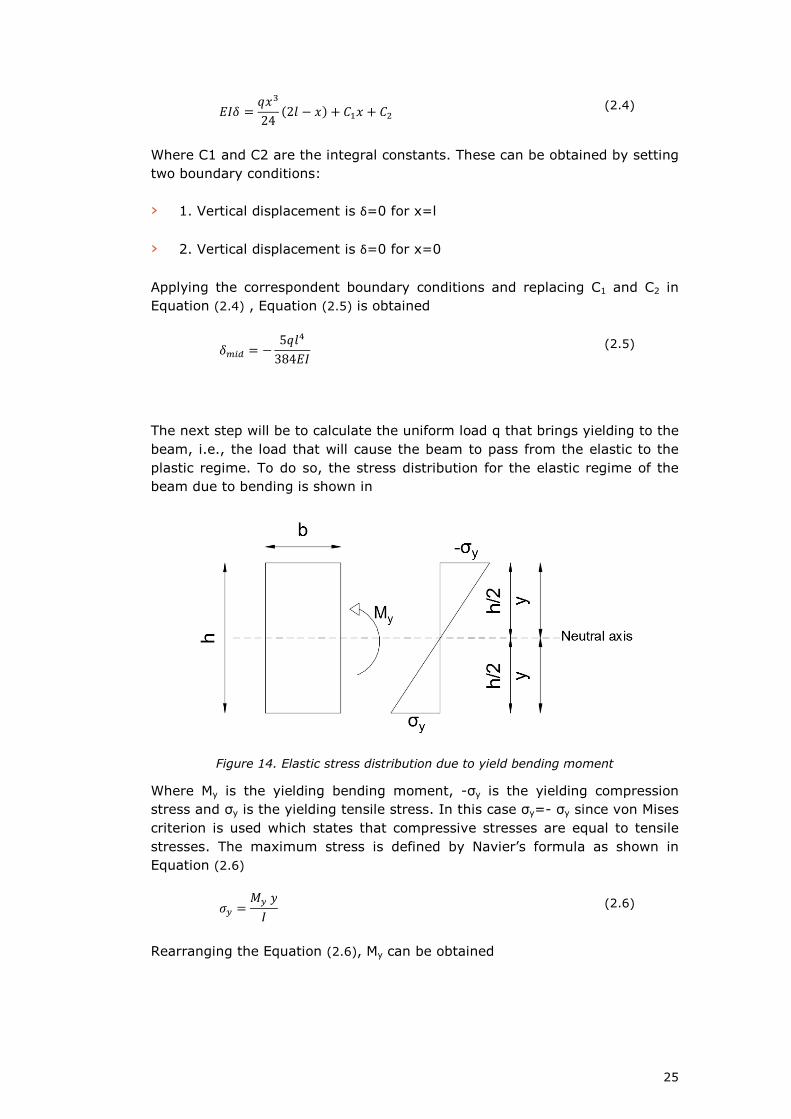
The next step will be to calculate the uniform load q that brings yielding to the
beam, i.e., the load that will cause the beam to pass from the elastic to the
plastic regime. To do so, the stress distribution for the elastic regime of the
beam due to bending is shown in
Figure 14. Elastic stress distribution due to yield bending moment
Where My is the yielding bending moment, -σy is the yielding compression
stress and σy is the yielding tensile stress. In this case σy=- σy since von Mises
criterion is used which states that compressive stresses are equal to tensile
stresses. The maximum stress is defined by Navier’s formula as shown in
Equation (2.6)
*+ = �+ ,� (2.6)
Rearranging the Equation (2.6), My can be obtained
26
�+ = *+ �, (2.7)
And the maximum bending moment in a simply supported beam subjected to
uniform load is equal to
�#-� = � �8 (2.8)
Equalizing Equations (2.7) and (2.8), qyielding can be obtained
�+ = 8 *+ �, � (2.9)
Results concerning the elastic behaviour of the plain concrete beam are shown
in Table 8
I
[mm4]
My
[Nmm]
qy
[N/mm]
qy ABAQUS
[N/mm2]
ẟmid
[mm]
2.6x10⁹ 2.6x10⁸ 20.83 0.083 33
Table 8. Plain concrete beam elastic regime results
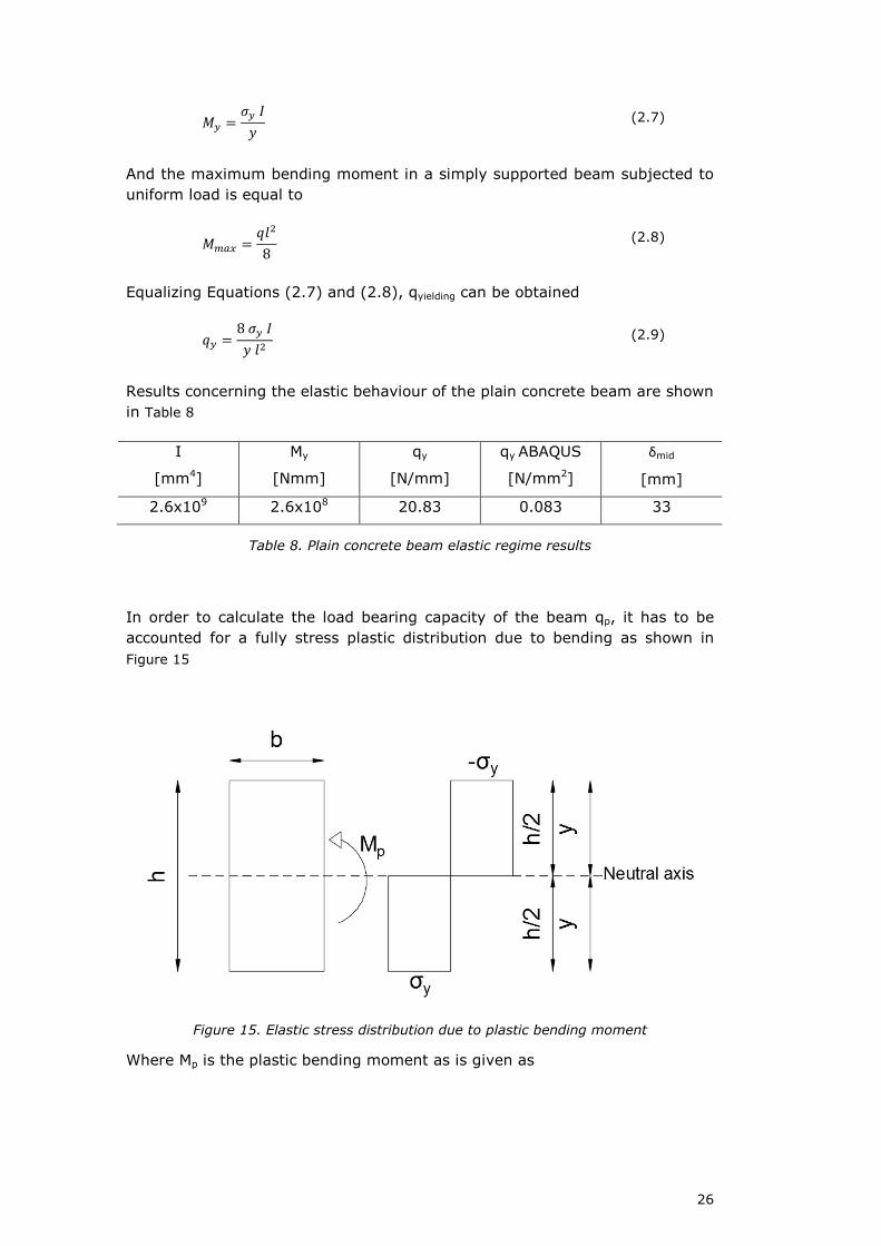
In order to calculate the load bearing capacity of the beam qp, it has to be
accounted for a fully stress plastic distribution due to bending as shown in
Figure 15
Figure 15. Elastic stress distribution due to plastic bending moment
Where Mp is the plastic bending moment as is given as

27
�. = *+ /� ℎ�4 0 (2.10)
Finally, Equation (2.9) (2.8) is rearranged and it is obtained
�. = 8 �1 � (2.11)
Results are presented in
Mp
[Nmm]
qp
[N/mm]
qp ABAQUS
[N/mm2]
3.9x10⁸ 31.25 0.125
Table 9. Plain concrete beam plastic regime results
2.2 NUMERICAL CALCULATIONS
Numerical solutions were performed in the software ABAQUS. Contrary to
analytical calculations, the plain concrete beam was modelled in 3d as a solid
body. Von Mises criteria was used to define the plasticity characteristics
shown in Table 7.
Boundary conditions are similar to the analytical solution. In one end is
restricted the horizontal and vertical displacement (ux=uy=0) and in the other
end it is restricted the vertical displacement (uy=0). Such boundary conditions
are applied at the same height of the neutral axis (h/2). Again, it is important
to remember that the beam is modelled along the axis z and not the axis x as
in the analytical static system. The plain concrete beam modelled can be
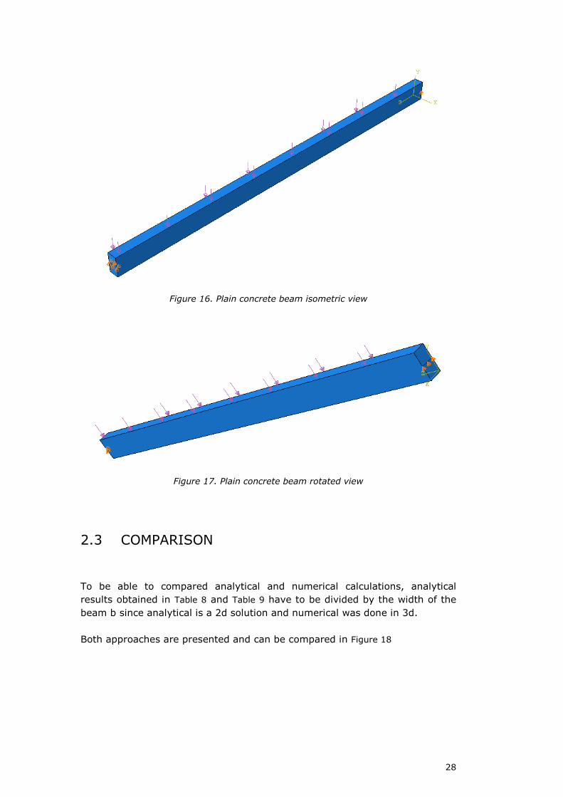
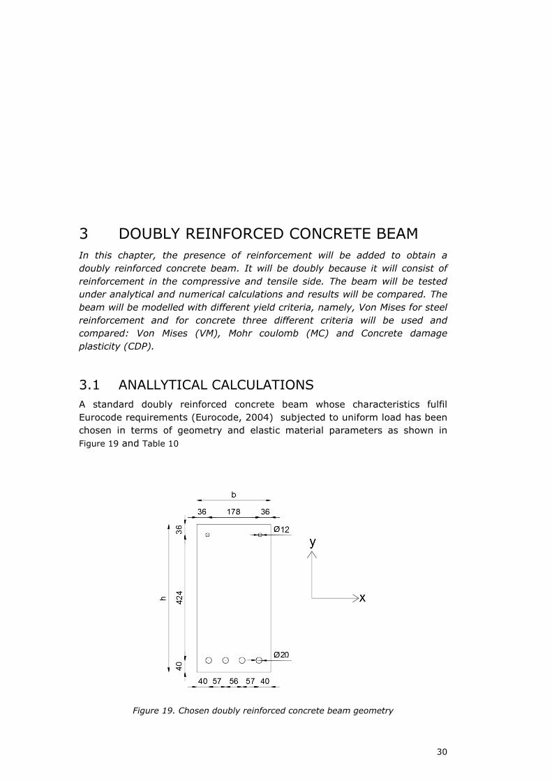
visualized in Figure 16 and Figure 17
28
Figure 16. Plain concrete beam isometric view
Figure 17. Plain concrete beam rotated view
2.3 COMPARISON
To be able to compared analytical and numerical calculations, analytical
results obtained in Table 8 and Table 9 have to be divided by the width of the
beam b since analytical is a 2d solution and numerical was done in 3d.
Both approaches are presented and can be compared in Figure 18

29
Figure 18. Plain concrete beam comparison results
It can be seen that qp matches perfectly the numerical solution. qy is also very
accurate although it is hard to know exactly when the elastic part ends and
the plastic starts. However, it has been also plotted the analytical elastic slope
and it is observed that is nearly similar to the numerical slope. It can be
concluded that when modelling plain concrete with von Mises criterion,
analytical and numerical calculations are practically similar.
30
3 DOUBLY REINFORCED CONCRETE BEAM
In this chapter, the presence of reinforcement will be added to obtain a
doubly reinforced concrete beam. It will be doubly because it will consist of
reinforcement in the compressive and tensile side. The beam will be tested
under analytical and numerical calculations and results will be compared. The
beam will be modelled with different yield criteria, namely, Von Mises for steel
reinforcement and for concrete three different criteria will be used and
compared: Von Mises (VM), Mohr coulomb (MC) and Concrete damage
plasticity (CDP).
3.1 ANALLYTICAL CALCULATIONS
A standard doubly reinforced concrete beam whose characteristics fulfil
Eurocode requirements (Eurocode, 2004) subjected to uniform load has been
chosen in terms of geometry and elastic material parameters as shown in
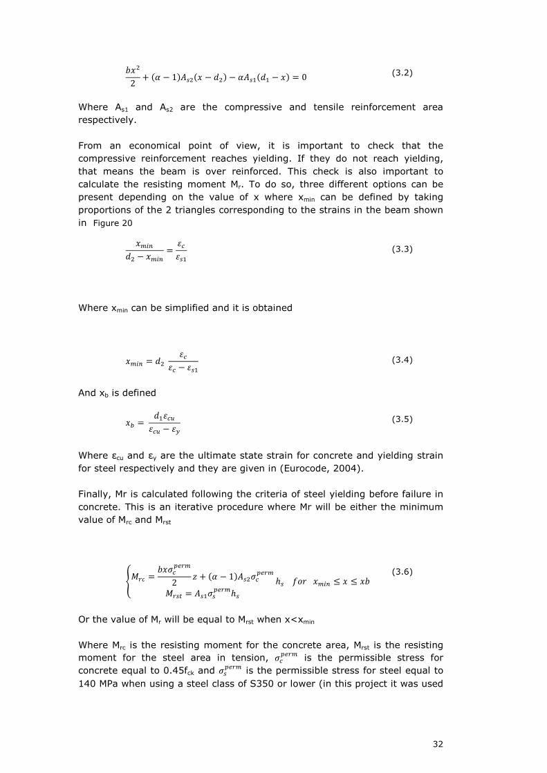
Figure 19 and Table 10
Figure 19. Chosen doubly reinforced concrete beam geometry

31
b
[mm]
h
[mm]
l
[mm]
ν (steel)
[-]
Es
[MPa]
Ec
[MPa]
ν (concrete)
[-]
250 500 104 0.30 2.1x10⁵ 31500 0.18
Table 10. Parameters for doubly reinforced concrete beam
The static system considered is similar to the one presented in Figure 12 for
the plain concrete beam being simply supported and subjected to an uniform
load q.
For SLS calculations, Alternate Design Method (ASD) will be used based on
(Jensen, 2011). This is a method based on elastic theory and thus, it is a
suitable for linear-elastic calculations.
To apply this method, steel is replaced by an equivalent concrete area
determined by their Young’s modulus (Es and Ec) that corresponds to the
modular ratio coefficient 2
2 = ��� (3.1)
This can be seen in Figure 20
Figure 20. ASD method representation
Where εs1 is the strain of the bars in the tensile zone, εs2 is the strain of the
bars in the compressive zone, εc is the strain of the concrete and x is the
distance from the upper edge to the neutral axis calculated with Equation
(3.2). This distance will correspond to the beam height in compression. This is
calculated by taking moments of area around the neutral axis.
32
���2 + �2 − 1���� − ��� − 2"��" − �� = 0 (3.2)
Where As1 and As2 are the compressive and tensile reinforcement area
respectively.
From an economical point of view, it is important to check that the
compressive reinforcement reaches yielding. If they do not reach yielding,
that means the beam is over reinforced. This check is also important to
calculate the resisting moment Mr. To do so, three different options can be
present depending on the value of x where xmin can be defined by taking
proportions of the 2 triangles corresponding to the strains in the beam shown
in Figure 20
�#$4�� − �#$4 = 5�5" (3.3)
Where xmin can be simplified and it is obtained
�#$4 = �� 5�5� − 5" (3.4)
And xb is defined
�6 = �"5�75�7 − 5+ (3.5)
Where εcu and εy are the ultimate state strain for concrete and yielding strain
for steel respectively and they are given in (Eurocode, 2004).
Finally, Mr is calculated following the criteria of steel yielding before failure in
concrete. This is an iterative procedure where Mr will be either the minimum
value of Mrc and Mrst
8�9� = ��*�.�9#2 : + �2 − 1��*�.�9#
�9; = "*.�9#ℎ< ℎ =>? �#$4 ≤ � ≤ �� (3.6)
Or the value of Mr will be equal to Mrst when x<xmin
Where Mrc is the resisting moment for the concrete area, Mrst is the resisting
moment for the steel area in tension, *�.�9# is the permissible stress for
concrete equal to 0.45fck and *.�9# is the permissible stress for steel equal to
140 MPa when using a steel class of S350 or lower (in this project it was used
33
a steel class of S345). These values were obtained from standard (ACI318M,
1995)
SLS results are presented in Table 11
Mrc
[Nmm]
qmrc
[N/mm]
ẟmrc
[mm]
εs1
[-]
εs2
[-]
εc
[-]
x
[mm]
69508917.58 5.56 7.75 0.014 0.0017 0.0035 122.23
Table 11. SLS Results ASD method doubly reinforced concrete beam
Another more recent method used for SLS calculation will be performed. It
will be calculated the deflection of the beam in the middle using Equation
(2.5). In this case the bending stiffness EI will be different; the cross section is
not symmetric and 2 different materials are merged (concrete and steel) to
form a composite material. Therefore, it is necessary account for the 2
materials when taking into account its resistance against bending. Neutral
axis will not be in the middle since the reinforcement on the top is different
from the reinforcement placed on the bottom.
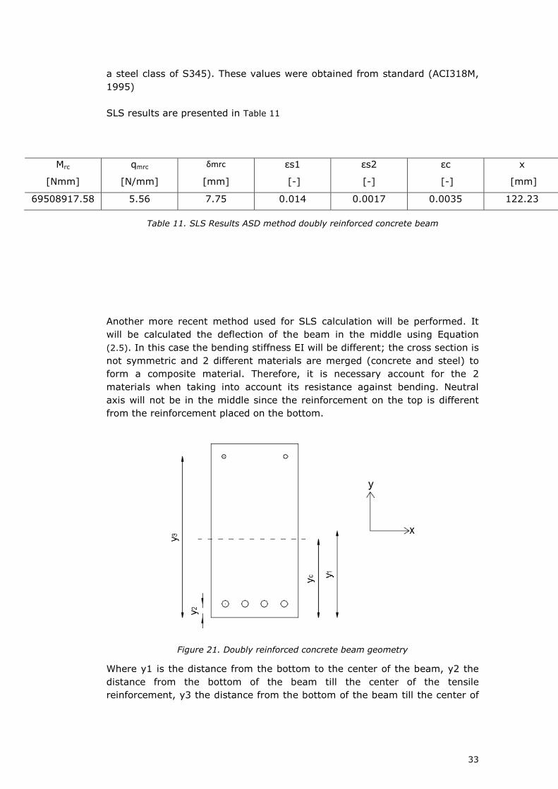
Figure 21. Doubly reinforced concrete beam geometry
Where y1 is the distance from the bottom to the center of the beam, y2 the
distance from the bottom of the beam till the center of the tensile
reinforcement, y3 the distance from the bottom of the beam till the center of

34
the compressive reinforcement and yc is the distance from the bottom of the
beam till the neutral axis.
The neutral axis position yc can be calculated as follows
,� = � ," �� − �" ,� + � ,�� ��� − ��� �� − �" + �� ��� − �� (3.7)
Where Ac is the concrete area including the holes and Ec and Es are the
concrete and steel Young’s Modulus respectively.
Next it can be obtained the second moment of inertia of the entire section Ics
�� = �� + ��," − ,��� − �AB"��B" + B"�,� − ,���� + AB� ��B� + B� �,� − ,���� (3.8)
Where nh1 and nh2 are the number of holes corresponding to compressive
and tensile reinforcement respectively, Ah1 and Ah2 is the singular hole area
for compressive and tensile reinforcement respectively, Ih1 and Ih2 are the
second moment of inertia of compressive and tensile reinforcement
respectively where Ih is equal to
�B = C D∅2F'4
(3.9)
Finally, the bending stiffness EI is obtained
�� = �� �� + AB"���B" + B"�,� − ,���� + AB����B� + B��,� − ,���� (3.10)
Where ∅ is the diameter of the steel bar. The SLS results are presented in
My
[Nmm]
qy
[N/mm]
ẟy
[mm]
69508917.58 2.08 2.83
Table 12. SLS results

35
For ULS calculations, it will be calculated the maximum capacity of the beam
subjected to bending which corresponds to the maximum bending moment
Mp. To do so, it is necessary to account for the stress-strain distribution on
the doubly reinforced concrete beam shown in Figure 22
Figure 22. Stress-strain distribution doubly reinforced concrete beam
Where λ is a factor defining the height of the compression zone, z is the
forces arm, y is the distance to the resultant compression force Cc, Cs is the
resultant force of the reinforcement in compression, Ts is the resultant of the
reinforcement in tension, η is a factor defining the effective strength of
concrete and Mp is the maximum moment in bending.
If horizontal equilibrium is established it is obtained
!� + ! = G (3.11)
Where
!� = =�H � λ� (3.12)
G = =" " (3.13)
! = =� � (3.14)
Being fs1 equal to the steel yielding stress fy=345MPa and fs2 is found by
Hook’s law
=� = � 5� (3.15)

36
Introducing equations 3.12, 3.13 and 3.14 into the equation 3.11 it is
obtained the distance to the neutral axis which divides compression from
tension zone
� = " =+ − � =�=�%J � (3.16)
Finally, it can be determined Mp by taking equilibrium of moments
�. = ! �, − ��� + G : (3.17)
The results are presented in Table 13
Mp
[Nmm]
qp
[N/mm]
ẟp
[mm]
260416666.7 14.92 20.79
Table 13. ULS results Doubly reinforced concrete beam
3.2 NUMERICAL CALCULATIONS
Numerical solutions were performed in the software ABAQUS. Contrary to
analytical calculations, the doubly reinforced concrete beam was modelled in
3d as a solid body. Von Mises, Mohr Coulomb, Concrete damage plasticity
criteria were used to define the plasticity of concrete whereas Von Misses
criterion was used to model steel. The parameters used to define Von Misses
for concrete and steel are
σy
[MPa]
εpl
[-]
25 0
Table 14. Von Misses parameters for concrete
σy
[MPa]
εpl
[-]
345 0
Table 15. Von Misses parameters for steel
37
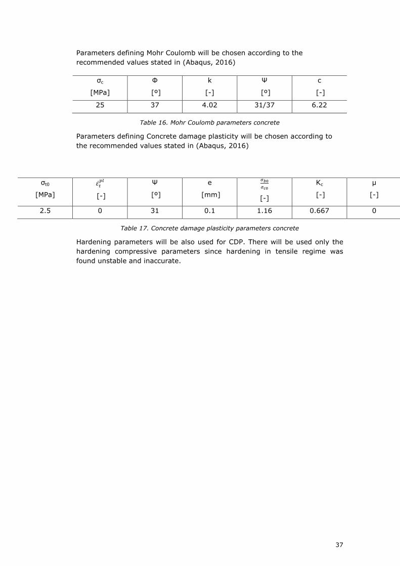
Parameters defining Mohr Coulomb will be chosen according to the
recommended values stated in (Abaqus, 2016)
σc
[MPa]
Φ
[º]
k
[-]
Ψ
[º]
c
[-]
25 37 4.02 31/37 6.22
Table 16. Mohr Coulomb parameters concrete
Parameters defining Concrete damage plasticity will be chosen according to
the recommended values stated in (Abaqus, 2016)
σt0
[MPa]
5K;.L [-]
Ψ
[º]
e
[mm]
MNOMPO [-]
Kc
[-]
µ
[-]
2.5 0 31 0.1 1.16 0.667 0
Table 17. Concrete damage plasticity parameters concrete
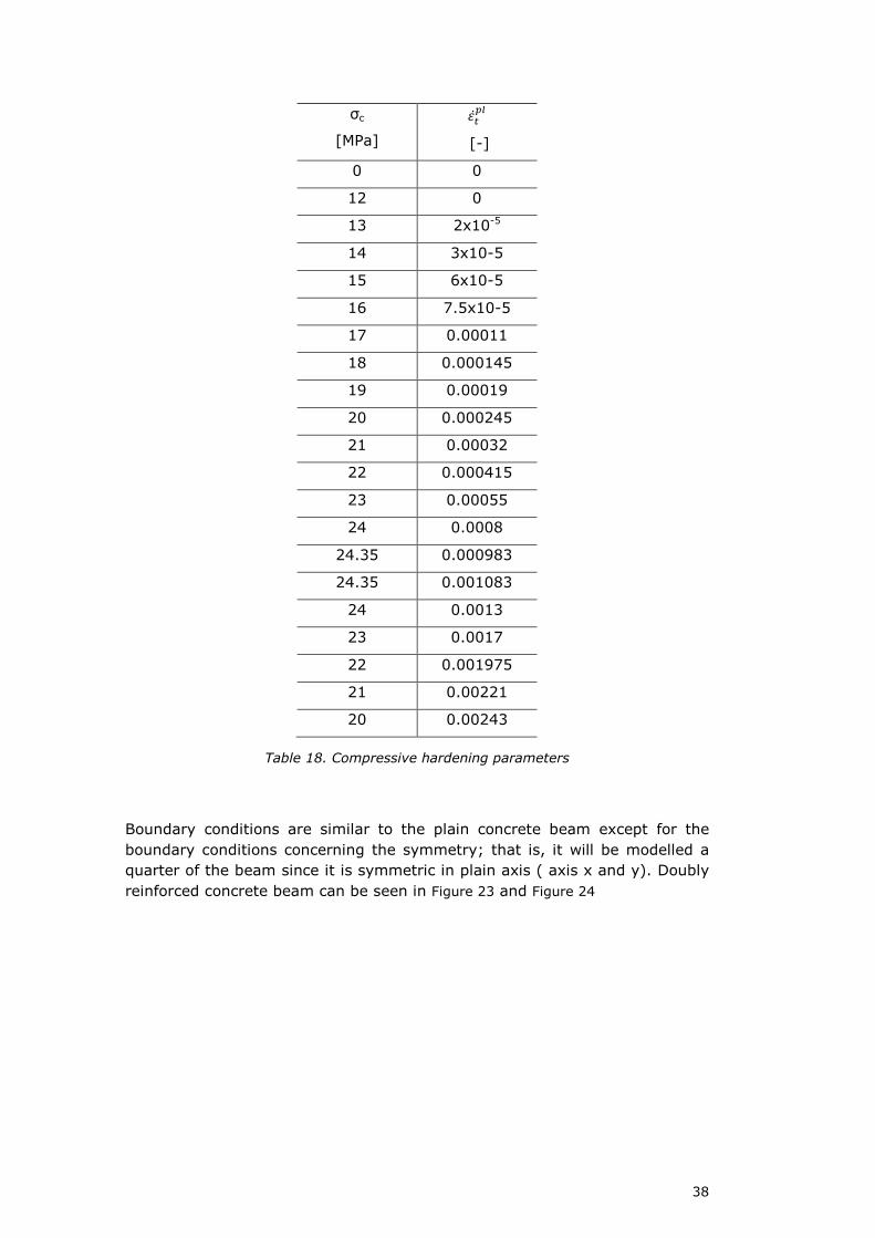
Hardening parameters will be also used for CDP. There will be used only the
hardening compressive parameters since hardening in tensile regime was
found unstable and inaccurate.
38
σc
[MPa]
5K;.L [-]
0 0
12 0
13 2x10⁻⁵
14 3x10⁻⁵
15 6x10⁻⁵
16 7.5x10⁻⁵
17 0.00011
18 0.000145
19 0.00019
20 0.000245
21 0.00032
22 0.000415
23 0.00055
24 0.0008
24.35 0.000983
24.35 0.001083
24 0.0013
23 0.0017
22 0.001975
21 0.00221
20 0.00243
Table 18. Compressive hardening parameters
Boundary conditions are similar to the plain concrete beam except for the
boundary conditions concerning the symmetry; that is, it will be modelled a
quarter of the beam since it is symmetric in plain axis ( axis x and y). Doubly
reinforced concrete beam can be seen in Figure 23 and Figure 24

39
Figure 23. Doubly reinforced concrete beam isometric view
Figure 24. Doubly reinforced concrete bam rotated view
3.3 COMPARISON
When comparing analytical and numerical results, it is important to take into
account that the load using in analytical calculations has been divided by the
width of the beam in order to compare results properly. This is because
analytical calculations are performed in a 2d beam and in numerical is 3d. The
results are presented in the next charts:

40
Figure 25. Von Misses concrete modelling
Figure 26. Abaqus Mohr Coulomb modelling

41
Figure 27. MC modelling dilation angle 37º and 31º
Figure 28. MC Modelling tension cut off 2.5
42
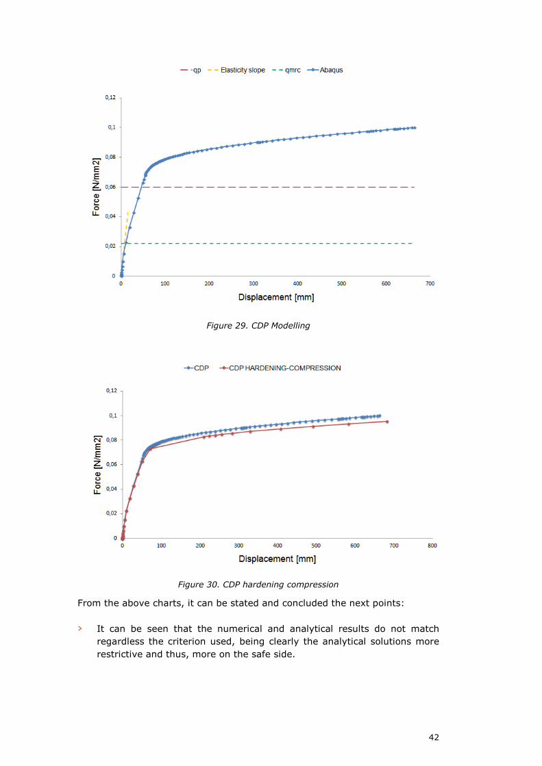
Figure 29. CDP Modelling
Figure 30. CDP hardening compression
From the above charts, it can be stated and concluded the next points:
› It can be seen that the numerical and analytical results do not match
regardless the criterion used, being clearly the analytical solutions more
restrictive and thus, more on the safe side.

43
› By performing the calculations analytically, it is made sure that the
structure is more resistant. However, it is also more expensive that it
should be.
› When using Mohr Coulomb criterion, it is observed that there is little
variation when changing the dilation angle from 37º to 31º.
› The most stable criterion is concrete damage plasticity that shows
correctly the elastic, elasto-plastic and plastic regime.

44
PART II-REINFORCED CONCRETE COLUMN

45
1 INTRODUCTION
In this part, a non-linear analysis of a plain and a reinforced concrete column
will be performed. It will be studied its failure by buckling. Analytical and
numerical solutions will be used and conclusions will be drawn.
46
2 PLAIN CONCRETE COLUMN
In this part, a non-linear analysis of a plain concrete column will be
performed. It will be studied its failure by buckling. Analytical and numerical
solutions will be used and conclusions will be drawn.
2.1 ANALLYTICAL CALCULATIONS
A standard plain concrete column whose characteristics fulfil Eurocode
requirements (Eurocode, 2004) subjected to axial uniform load. Its elastic
and plastic parameters are similar to the ones used with the doubly reinforced
concrete beam. It is going to be studied the column resistance against
buckling. Buckling is a type of deformation as a result of axial compression
loads. This leads to have eccentricity in the column (bending). This will occur
at lower stress levels than the ultimate normal stress of the column. Buckling
depends on many factors like the shape of the column, slenderness, grade of
construction imperfection and boundary conditions.
Its geometry and static system of the column that will be analyzed is shown
below
47
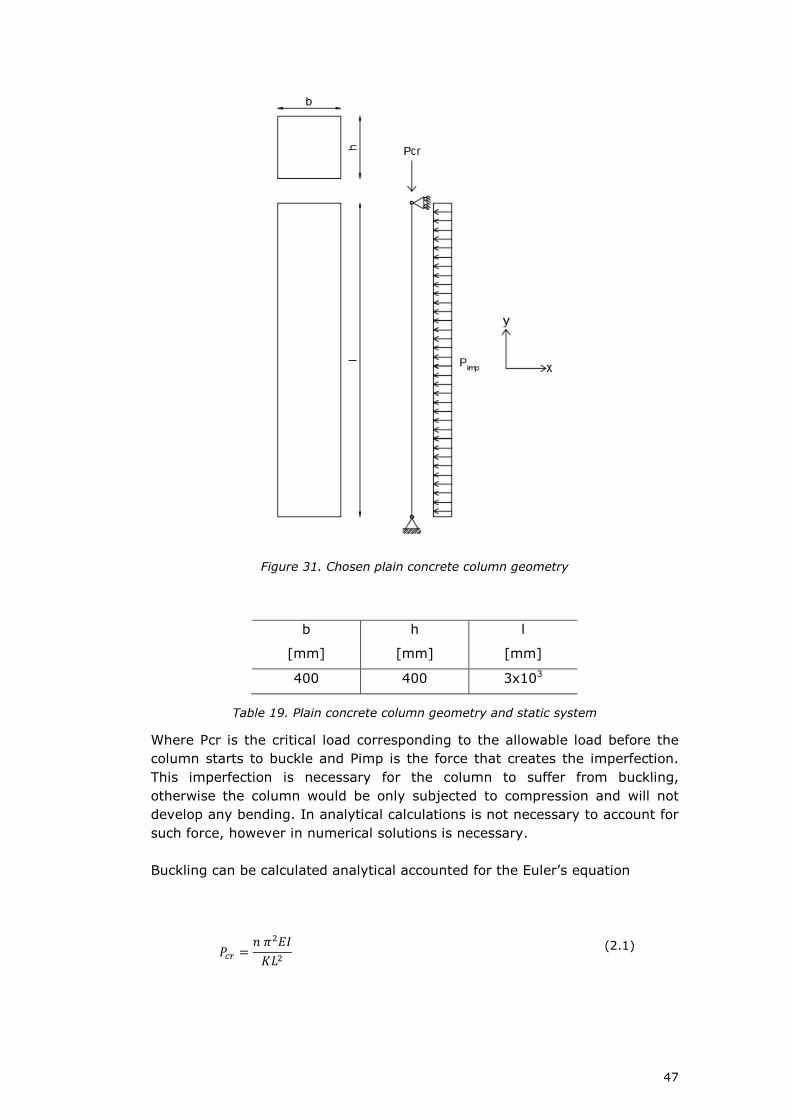
Figure 31. Chosen plain concrete column geometry
b
[mm]
h
[mm]
l
[mm]
400 400 3x10³
Table 19. Plain concrete column geometry and static system
Where Pcr is the critical load corresponding to the allowable load before the
column starts to buckle and Pimp is the force that creates the imperfection.
This imperfection is necessary for the column to suffer from buckling,
otherwise the column would be only subjected to compression and will not
develop any bending. In analytical calculations is not necessary to account for
such force, however in numerical solutions is necessary.
Buckling can be calculated analytical accounted for the Euler’s equation
Q�9 = A C���RS� (2.1)
48
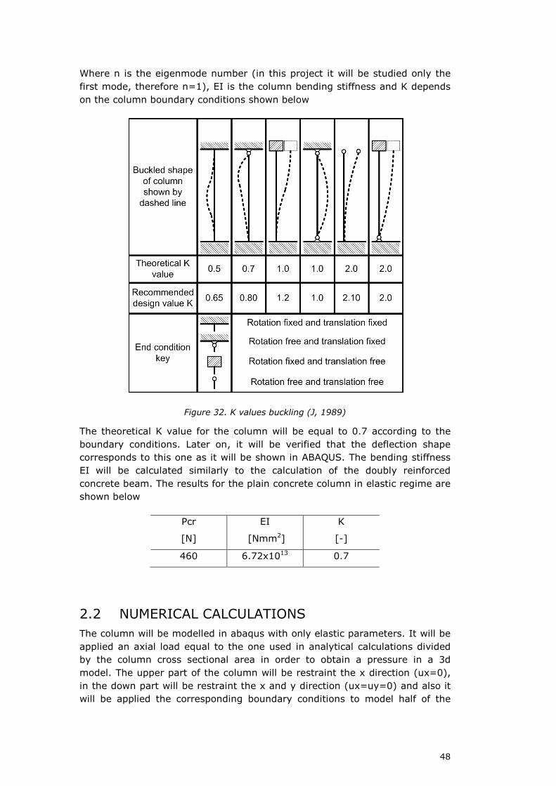
Where n is the eigenmode number (in this project it will be studied only the
first mode, therefore n=1), EI is the column bending stiffness and K depends
on the column boundary conditions shown below
Figure 32. K values buckling (J, 1989)
The theoretical K value for the column will be equal to 0.7 according to the
boundary conditions. Later on, it will be verified that the deflection shape
corresponds to this one as it will be shown in ABAQUS. The bending stiffness
EI will be calculated similarly to the calculation of the doubly reinforced
concrete beam. The results for the plain concrete column in elastic regime are
shown below
Pcr
[N]
EI
[Nmm2]
K
[-]
460 6.72x10¹³ 0.7
2.2 NUMERICAL CALCULATIONS
The column will be modelled in abaqus with only elastic parameters. It will be
applied an axial load equal to the one used in analytical calculations divided
by the column cross sectional area in order to obtain a pressure in a 3d
model. The upper part of the column will be restraint the x direction (ux=0),
in the down part will be restraint the x and y direction (ux=uy=0) and also it
will be applied the corresponding boundary conditions to model half of the

49
beam (symmetry). Finally the 2 loads Pcr and Pimp will be applied to the
column.
Figure 33. Abaqus plain concrete column
2.3 COMPARISON
Both results, analytical and numerical, can be compared observing the
following graph
50
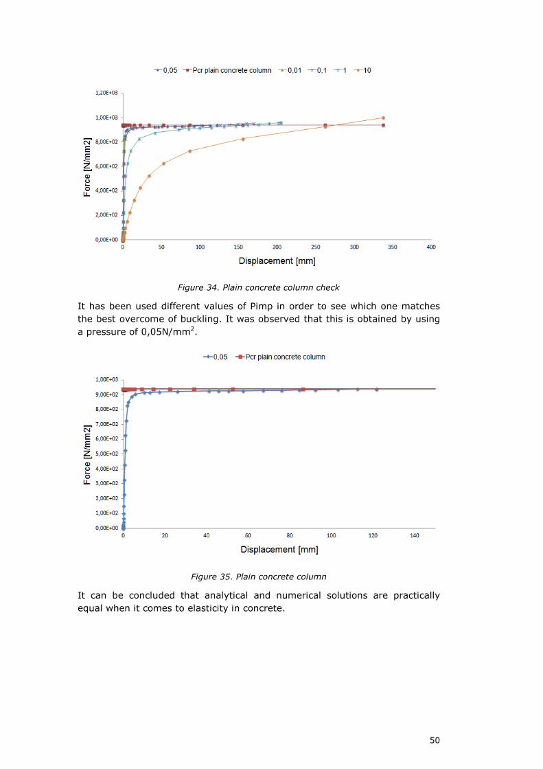
Figure 34. Plain concrete column check
It has been used different values of Pimp in order to see which one matches
the best overcome of buckling. It was observed that this is obtained by using
a pressure of 0,05N/mm2.
Figure 35. Plain concrete column
It can be concluded that analytical and numerical solutions are practically
equal when it comes to elasticity in concrete.

51
3 REINFORCED CONCRETE COLUMN
In this part, a non-linear analysis of a reinforced concrete column will be
performed. It will be studied its failure by buckling. Analytical and numerical
solutions will be used and conclusions will be drawn.
3.1 ANALLYTICAL CALCULATIONS
Analytical calculations for a reinforced concrete column within the elastic
regime are similar to plain concrete. The only difference is a variation of the
bending stiffness EI due to the addition of steel to form a composite material.
Bending stiffness will be calculated similarly as the doubly reinforced concrete
beam and the cross sectional area geometry in mm can be seen below
Figure 36. Reinforced concrete column cross sectional area
The results for the elastic reinforced concrete column can be seen in
Pcr
[N]
EI
[Nmm2]
K
[-]
477 6.96x10¹³ 0.7
Table 20. Reinforced concrete column elastic results
52
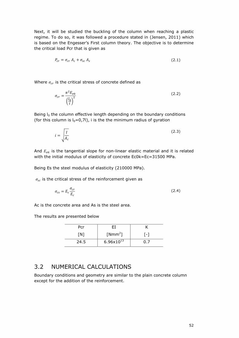
Next, it will be studied the buckling of the column when reaching a plastic
regime. To do so, it was followed a procedure stated in (Jensen, 2011) which
is based on the Engesser’s First column theory. The objective is to determine
the critical load Pcr that is given as
Q�9 = *�9 � + *� (2.1)
Where *�9 is the critical stress of concrete defined as
*�9 = C��MHD TU F� (2.2)
Being l0 the column effective length depending on the boundary conditions
(for this column is l0=0,7l), i is the the minimum radius of gyration
U = V �� (2.3)
And �MH is the tangential slope for non-linear elastic material and it is related
with the initial modulus of elasticity of concrete Ec0k=Ec=31500 MPa.
Being Es the steel modulus of elasticity (210000 MPa).
*� is the critical stress of the reinforcement given as
*� = � *�9�� (2.4)
Ac is the concrete area and As is the steel area.
The results are presented below
Pcr
[N]
EI
[Nmm2]
K
[-]
24.5 6.96x10¹³ 0.7
3.2 NUMERICAL CALCULATIONS
Boundary conditions and geometry are similar to the plain concrete column
except for the addition of the reinforcement.
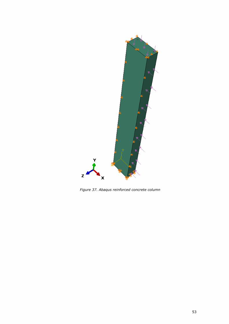
53
Figure 37. Abaqus reinforced concrete column
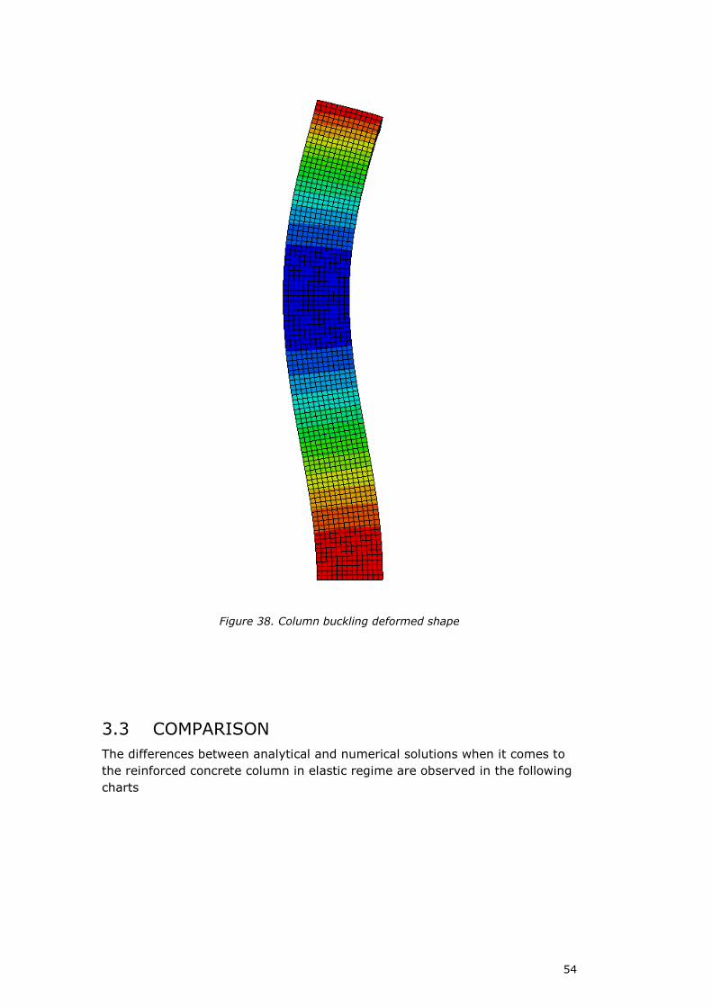
54
Figure 38. Column buckling deformed shape
3.3 COMPARISON
The differences between analytical and numerical solutions when it comes to
the reinforced concrete column in elastic regime are observed in the following
charts
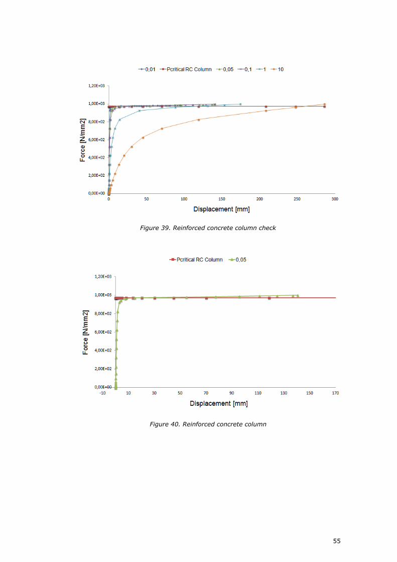
55
Figure 39. Reinforced concrete column check
Figure 40. Reinforced concrete column

56
Figure 41. Plain and reinforced concrete column
Once more, it can be seen that when having an elastic behaviour, analytical
and numerical solutions are highly similar.
The differences between analytical and numerical solutions when it comes to
the reinforced concrete column in elasto-plastic regime are observed in the
next charts
Figure 42. Von Misses reinforced concrete column
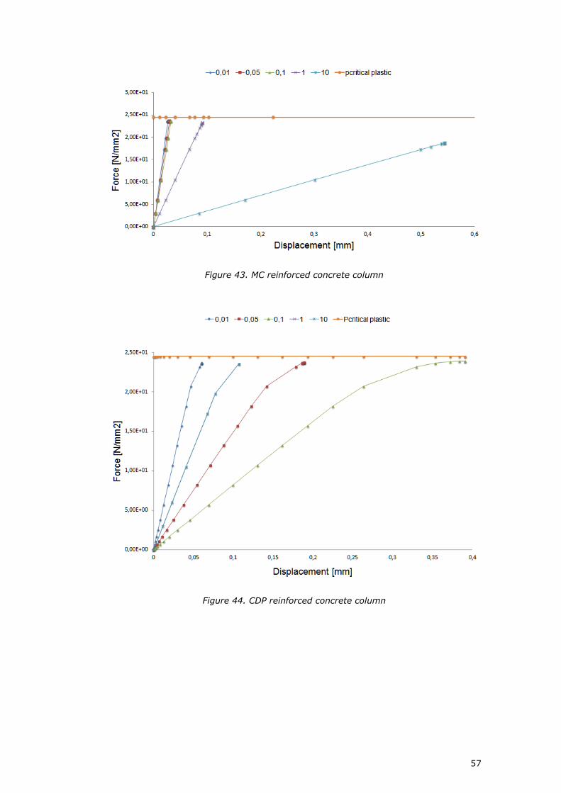
57
Figure 43. MC reinforced concrete column
Figure 44. CDP reinforced concrete column

58
PART III-CONCLUSION
59
1 CONCLUSIONS
Once checked all the analytical and numerical results, the next conclusions
can be drawn:
› It has been observed that numerical solutions for the doubly reinforced
concrete beam are less similar than for the study of buckling in the
reinforced concrete column. It seems, this is due to the fact that studying
bending for a composite material is a more complex matter since there
are more assumptions made in the calculations.
› In general, Von Mises and Concrete Damage Plasticity criteria are more
stable and accurate than Mohr Coulomb.
› All in all, analytical and numerical solutions appear to be significantly
similar for linear elastic and non-linear behaviour.
› Numerical solutions take more time than analytical solutions. From an
economical point of view, it can be concluded that it is preferable to use
analytical calculations than numerical since they appear to give roughly
similar results.
› The use of stirrups might vary the results. This can be important for
further research.

60
REFERENCES
61
Abaqus, 2016. Abaqus Manual 2016. s.l.:s.n.
ACI318M, 1995. Building code requirements for reinforced concrete. s.l.:s.n.
Continuummechanics, 2011.
http://www.continuummechanics.org/vonmisesstress.html. [Online].
Eurocode, 2004. Eurocode 3: Design of steel structures-Part 1-9: Fatigue, s.l.: s.n.
Eurocode, 2004. Eurocode2: Design of concrete structures - Part 1-1: General rules
and rules for buuildings, s.l.: European standard.
Iverson, B., Bauer, S. & Flueckiger, S., 2014. Thermocline bed properties for
deformation analysis. [Online].
Jensen, B. C., 2011. Concrete structures. Horsens: s.n.
J, L., 1989. A Plastic damage model for concrete, s.l.: International Journal of solids
and structures.
Lee, J., 1998. Plastic damage model for cyclic loading of concrete structures, s.l.:
Journal of engineering mechanics.
Ottosen, N. S., 2005. The Mechanics of Constitutive Modelling. Elsevier: s.n.
software, C. e., 2013. http://www.finesoftware.eu/help/geo5/en/mohr-coulomb-
model-with-tension-cut-off-01/. [Online].
Wikimedia.org, 2004. http://www.constructionchat.co.uk/articles/heaviest-concrete-
structures-in-the-world/. [Online].
Wikipedia, 2016. Wikipedia. [Online]
Available at: https://en.wikipedia.org/wiki/Fatigue_(material)
Wikipedia, 2017.
https://en.wikipedia.org/wiki/Euler%E2%80%93Bernoulli_beam_theory. [Online].
Wikipedia, 2017. https://en.wikipedia.org/wiki/Series_and_parallel_springs. [Online].
wikipedia, 2017. https://en.wikipedia.org/wiki/Von_Mises_yield_criterion. [Online].
Yun, X. & Gardner, L., 2017. Stress strain curves for hot-rolled steels. s.l.:s.n.
62
APPENDIX A: YIELD CRITERIA THEORY
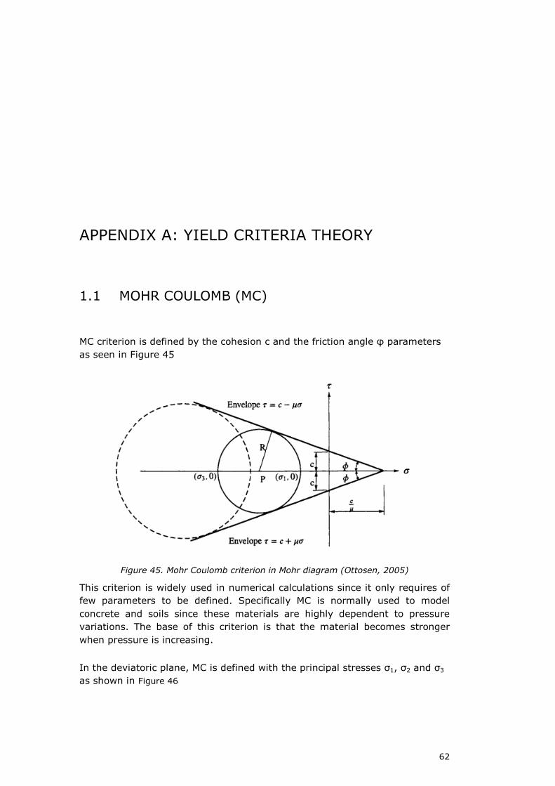
1.1 MOHR COULOMB (MC)
MC criterion is defined by the cohesion c and the friction angle φ parameters
as seen in Figure 45
Figure 45. Mohr Coulomb criterion in Mohr diagram (Ottosen, 2005)
This criterion is widely used in numerical calculations since it only requires of
few parameters to be defined. Specifically MC is normally used to model
concrete and soils since these materials are highly dependent to pressure
variations. The base of this criterion is that the material becomes stronger
when pressure is increasing.
In the deviatoric plane, MC is defined with the principal stresses σ1, σ2 and σ3
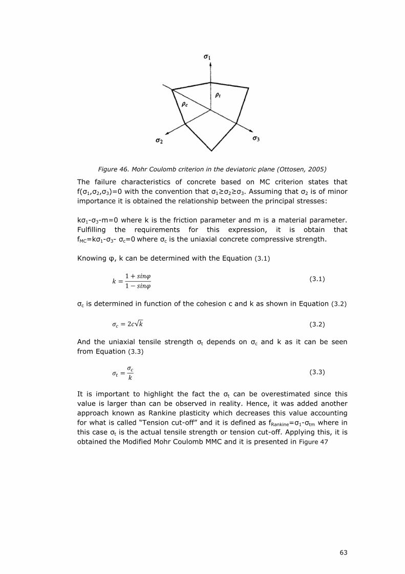
as shown in Figure 46
63
Figure 46. Mohr Coulomb criterion in the deviatoric plane (Ottosen, 2005)
The failure characteristics of concrete based on MC criterion states that
f(σ1,σ2,σ3)=0 with the convention that σ1≥σ2≥σ3. Assuming that σ2 is of minor
importance it is obtained the relationship between the principal stresses:
kσ1-σ3-m=0 where k is the friction parameter and m is a material parameter.
Fulfilling the requirements for this expression, it is obtain that
fMC=kσ1-σ3- σc=0 where σc is the uniaxial concrete compressive strength.
Knowing φ, k can be determined with the Equation (3.1)
� = 1 + WUAX1 − WUAX (3.1)
σc is determined in function of the cohesion c and k as shown in Equation (3.2)
*� = 2Y√� (3.2)
And the uniaxial tensile strength σt depends on σc and k as it can be seen
from Equation (3.3)
*; = *�� (3.3)
It is important to highlight the fact the σt can be overestimated since this
value is larger than can be observed in reality. Hence, it was added another
approach known as Rankine plasticity which decreases this value accounting
for what is called “Tension cut-off” and it is defined as fRankine=σ1-σtm where in
this case σt is the actual tensile strength or tension cut-off. Applying this, it is
obtained the Modified Mohr Coulomb MMC and it is presented in Figure 47

64
Figure 47. a) Rankine yield condition in the deviatoric plane, b) Modified Mohr coulomb
criterion (software, 2013)
Therefore, in the case of ccotgφ>σt, the tensile strength of the material σt is
set to the tension cut off.
Another parameter that is needed to define this criterion is the dilation angle
ψ, which is related to the volumetric strain of the material εv as shown in
Figure 48
Figure 48. a) friction angle representation, b) dilation angle representation (Iverson, et
al., 2014)
1.2 CONCRETE DAMAGE PLASTICITY (CDP)
This constitutive model is found in software ABAQUS and it is indicated mainly
for solving concrete structures and others quasi-brittle materials (Abaqus,
2016). CDP yield surface is shown in Figure 49

65
Figure 49. CDP in a) Deviatoric plane b) Plane stress plane (Abaqus, 2016)
CDP can be understood as a modification of the Drucker-Prager criterion by
changing the circular failure surface by a shape defined with the parameter kc.
Its yield function was stated by (J, 1989) and posteriously, some corrections
were made by (Lee, 1998). The yield function is provided in (3.4)
= = 11 − 2 [� − 32\ + ]�5K.L�*#-� − ^�−*#-��_ − *�[5K�.L_ = 0 (3.4)
Where
2 = `*6T*�Ta − 12 `*6T*�Ta − 1 , 0 ≤ 2 ≤ 0.5
(3.5)
and
] = *� [5K�.L_*; [5K;.L_ �1 − 2� − �1 + 2� (3.6)
Being γ
^ = 3�1 − R��2R� − 1 (3.7)
Where σmax is the maximum principal effective stress, σb0/σc0 is the ratio of
initial equibiaxial compressive yield stress to initial uniaxial compressive yield
stress, Kc is the ratio of the second stress invariant on the tensile meridian
q(TM) to the compressive meridian q(CM) at yield for any pressure p, *; [5K;.L_ is the effective tensile cohesion stress and *� [5K�.L_ is the effective compressive
cohesion stress.

66
The main purpose of the CDP model is to deal with stiffness recovery when
subjected to dynamic loading (Abaqus, 2016). The stress strain curve based
on CDP is shown in Figure 50
Figure 50. a) Uniaxial loading in compression , b) Uniaxial loading in tension (Abaqus,
2016)
In a) it can be observed that there is an initial elastic regime marked with a
straight line corresponding to the Youngs modulus E, thereafter the plastic
regime starts to be developed from the yield compressive stress σc0 until it
reaches the ultimate compressive stress σcu and finally, concrete undergoes
softening.
In b) it can be appreciated a similar behaviour to a) except for the fact that
the yield stress is equal to the ultimate tensile stress σt0.
1.3 VON MISES (VM)
Von misses yield criterion is usually used for ductile materials like metals. The
von Misses stress is calculated and then it is compared with the yield stress to
the material to check if the yield limit has been exceeded. The VM yield
surface in principal stress coordinates correspond to a circular cylinder as can
be observed in Figure 51
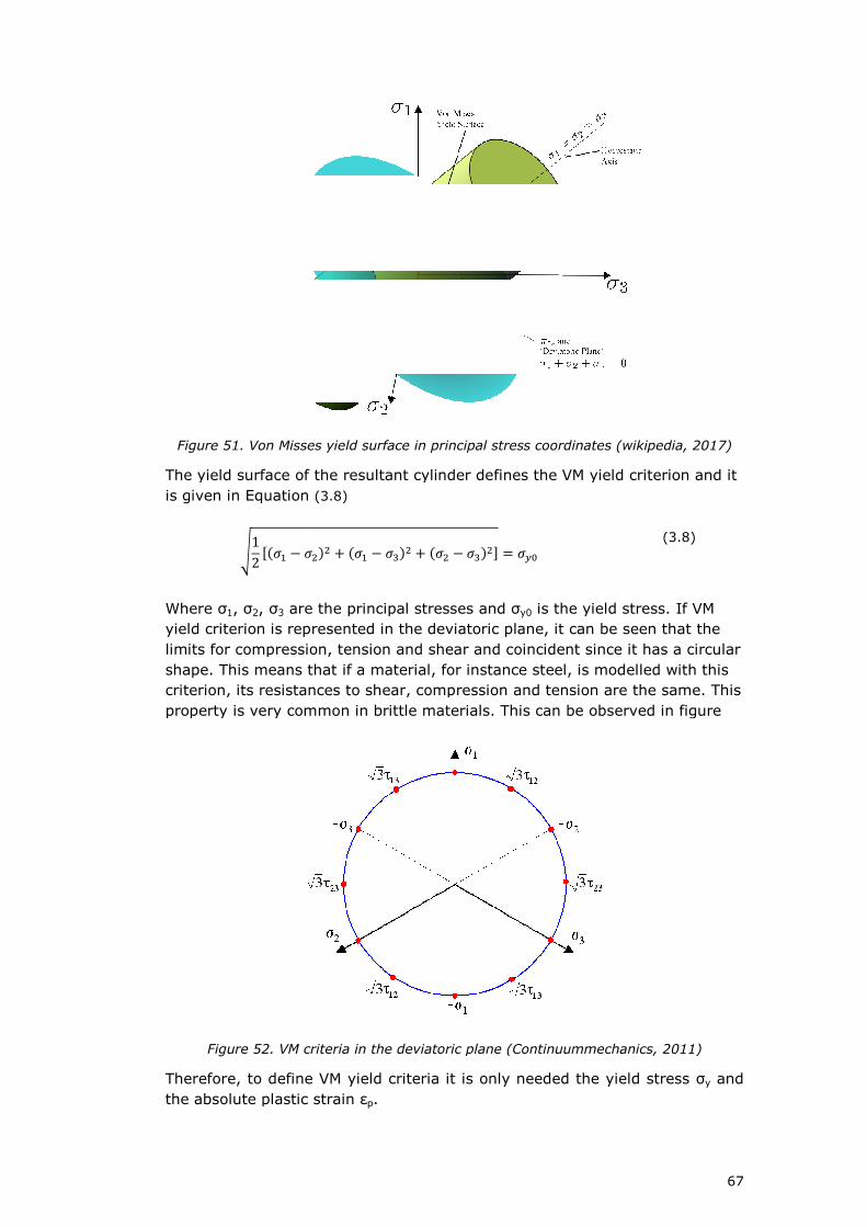
Figure 51. Von Misses yield surface in principal stress coordinates
The yield surface of the resultant cylinder defines the VM yield criterion and it
is given in Equation
V12d�*" � *�
Where σ1, σ2, σ3 are the principal stresses and σ
yield criterion is represented in the deviatoric plane, it can be seen that the
limits for compression, tension and shear and coincident since it has a circular
shape. This means that if a material, for instance steel, is modelled with this
criterion, its resistances to shear, compression and tension are the same. This
property is very common in brittle materials. This can be observed in figure
Figure 52. VM criteria in the deviatoric plane
Therefore, to define VM yield criteria it is only needed the yield stress σ
the absolute plastic strain ε
. Von Misses yield surface in principal stress coordinates (wikip
The yield surface of the resultant cylinder defines the VM yield criterion and it
is given in Equation (3.8)
��� � �*" � *��
� � �*� � *���e � *+T
are the principal stresses and σy0 is the yield stress. If VM
yield criterion is represented in the deviatoric plane, it can be seen that the
limits for compression, tension and shear and coincident since it has a circular
e. This means that if a material, for instance steel, is modelled with this
criterion, its resistances to shear, compression and tension are the same. This
property is very common in brittle materials. This can be observed in figure
. VM criteria in the deviatoric plane (Continuummechanics, 2011)
Therefore, to define VM yield criteria it is only needed the yield stress σ
the absolute plastic strain εp.
67
(wikipedia, 2017)
The yield surface of the resultant cylinder defines the VM yield criterion and it
(3.8)
is the yield stress. If VM
yield criterion is represented in the deviatoric plane, it can be seen that the
limits for compression, tension and shear and coincident since it has a circular
e. This means that if a material, for instance steel, is modelled with this
criterion, its resistances to shear, compression and tension are the same. This
property is very common in brittle materials. This can be observed in figure
(Continuummechanics, 2011)
Therefore, to define VM yield criteria it is only needed the yield stress σy and

68

69
APPENDIX B: RESULTS VERIFICATION
CONCRETE-STEEL SAMPLE
As=π∗r2=78.54mm2
Ac=b*h-π∗r2=321.46mm2
ux=F/kc+ks=0.03756mm
CONCRETE-STEEL-CONCRETE SAMPLE
As=π∗r2=78.54mm2
Ac=b*h=400mm2
ux=F/kc+ks=0.03437mm
CONCRETE SAMPLE
As=0
Ac=b*h=400mm2
ux=F/(kc+ks)=0.07936mm
70
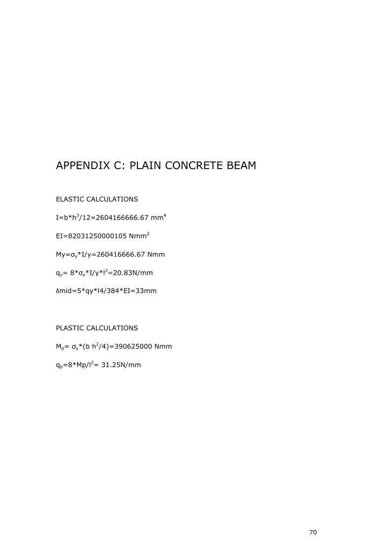
APPENDIX C: PLAIN CONCRETE BEAM
ELASTIC CALCULATIONS
I=b*h3/12=2604166666.67 mm4
EI=82031250000105 Nmm2
My=σy*I/y=260416666.67 Nmm
qy= 8*σy*I/y*l2=20.83N/mm
ẟmid=5*qy*l4/384*EI=33mm
PLASTIC CALCULATIONS
Mp= σy*(b h2/4)=390625000 Nmm
qp=8*Mp/l2= 31.25N/mm

71
APPENDIX D: REINFORCED CONCRETE BEAM
CALCULATION OF X
As1=1256.63 mm2
As2=226.20 mm2
2 � 6.67
x=122.23 mm
xmin=66.32 mm
xb=247.06mm
STRAINS CALCULATIONS
εcu=0.035
εy=0.0016
εs1=0.014
εs2=0.0017
MOMENTS CALCULATIONS
Mrc=69508917.58 Nmm
Mrst=74593200,64 Nmm

72
BEAM DISTANCES
Yc=240.85mm
Y1=250mm
Y2=40mm
Y3=464mm
Ics=2604166667mm4
Ic=2552650899mm4
Ih1=7853.98mm4
Ih2=1017.87mm4
SLS RESULTS
EI=9.34X10¹³ MPa
qmrc=5.56 N/mm
ẟmrc=7.75 mm
My=69508917.58 Nmm
qy=2.08 N/mm
ẟy=20.79mm
ULS RESULTS
Cs=78037.21 N
Ts=433535.28 N
x=71.09 mm
Mp=186506578.9 Nmm
qp=14.92 N/mm

73
ẟp=20.79mm
η=1
λ=0.8
NUMERICAL CALCULATIONS
VON MISES
σy=25 MPa
εpl=0
σy=345 MPa
εpl=0
MOHR COULOMB
σc=25 MPa
Φ=37º
K=4.02
Ψ=31º/37º
C=6.22
CONCRETE DAMAGE PLASTICITY
σt0=2.5
ε tpl =0
ψ=31º
e=0.1mm
σb0/σc0=1.16
Kc=0.667
µ=0
74
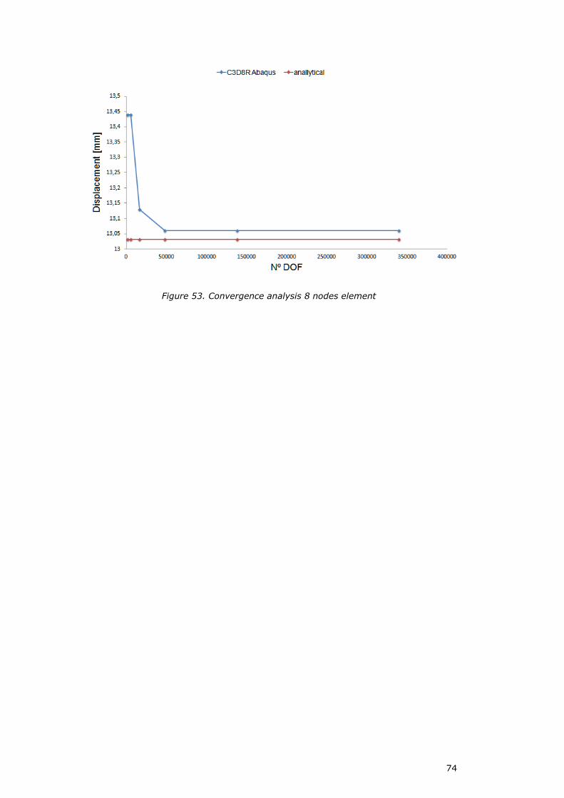
Figure 53. Convergence analysis 8 nodes element
75
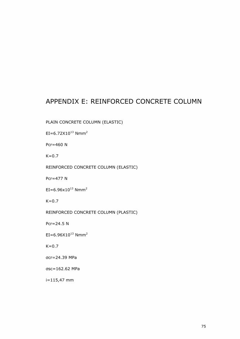
APPENDIX E: REINFORCED CONCRETE COLUMN
PLAIN CONCRETE COLUMN (ELASTIC)
EI=6.72X10¹³ Nmm2
Pcr=460 N
K=0.7
REINFORCED CONCRETE COLUMN (ELASTIC)
Pcr=477 N
EI=6.96x10¹³ Nmm2
K=0.7
REINFORCED CONCRETE COLUMN (PLASTIC)
Pcr=24.5 N
EI=6.96X10¹³ Nmm2
K=0.7
σcr=24.39 MPa
σsc=162.62 MPa
i=115,47 mm


