Chapter 1 CAPITAL INVESTMENT APPRAISAL Learning outcomes After studying this chapter candidates must be able to: Demonstrate knowledge of key investment, regarding appraisal methods and the following. The concept of the time value of money Net present value (NPV) Real and normal interest rates Payback Internal rate of return Multiple IRRs Unequal Project appraisal & Audit INTRODUCTION Capital Budgeting involves the assessment of how much should be spent on assets or project and which assets should be acquired. Before deciding which project/assets to invest in, corporations must compare the benefits to be derived from the acquisition/investment against the costs involved in the investment. The investment will not purely depend upon financial aspects but to a large extent, the strategic direction of the business. Remember the financial decisions fall with the long-term corporate strategy formulation process. 1
Transcript
Chapter 1
CAPITAL INVESTMENT APPRAISAL
Learning outcomes
After studying this chapter candidates must be able to: Demonstrate knowledge of key investment, regarding appraisal methods and the following.
The concept of the time value of money Net present value (NPV) Real and normal interest rates Payback Internal rate of return Multiple IRRs Unequal Project appraisal & Audit
INTRODUCTION
Capital Budgeting involves the assessment of how much should be spent on assets or project and which assets should be acquired.
Before deciding which project/assets to invest in, corporations must compare the benefits to be derived from the acquisition/investment against the costs involved in the investment.
The investment will not purely depend upon financial aspects but to a large extent, the strategic direction of the business. Remember the financial decisions fall with the long-term corporate strategy formulation process.
Appraisal Methods
The main methods of investment appraisal, which are normally in use, are:
(a) Payback (b) Internal rate of return (c) Net present value (d) Accounting rate of return.
1
The investment appraisal methods can be divided into traditional and scientific methods. The traditional methods ignore the fine value of money whilst the scientific methods recognise the fine value of money in the evaluation.
Net Present Value (NPV)
The Net Present Value of a project is the difference between the sum of the project discounted cash inflows and outflows attributable to a capital investment or other long-term project.
The Net Present Value approach holds that cash received in the future is less valuable than cash received today.
In the Net Present value computations, all cash flows are expressed in present day values by the cash flows, which are realised in the future.
A comparison is then made, in present day terms of the total costs of the investment (cash outflows) and the total receipts from the investment (cash inflows).
When the present value of the inflows exceeds that of outflows (which includes any relevant taxation liabilities, as well as the more obvious initial investment outlay), the net present value is positive and purely on financial grounds, the investment should be accepted. In contrast, if the present value of the outflows exceeds the present value of inflows, the net present value is negative and the investment should be rejected.
Discount Factors/ Interest Rate
The interest rate, at which investors can borrow or lend money, is key to the Net Present Value model (NPV). The model is based on the assumption that an investor may invest money in the financial market at an interest rate prevailing or invest money in real assets, undertake a combination of the two options, or borrow in order to invest in real asset.
Real assets will only be attractive to a rational investor if they offer a rate of return in excess of the cost of money (the rate at which the money has been borrowed).
By discounting the financial costs and benefits associated with real assets at this rate, the investor can determine whether a return in excess of discount rate ‘r’ is available from the real asset in question.
NPV and The Agency Theory
Senior managers of an organisation normally save the interests of shareholders and they are thereby employed to maximise the wealth of shareholders.
Since Net present Value models decision rule advocates that a project whose financial benefits outweigh its financial cost, henceforth having a positive net present value should
2
be accepted and be pursued and vice versa. The net present value upholds the thenetical sole objective of business of maximisation of shareholder’s wealth through maximisation of returns from the project.
Assumption in Net Present Value
The Net Present Value technique is based on the following assumption.
The Discount rate must be a measure of the opportunity cost of funds for wealth maximisation to result.
Perfect capital market and perfect information exists The model assumes that a single rate which reflects the opportunity cost for all
individuals and companies. All Shareholders have an objective of wealth maximisation
Net Present Value, Risk and Uncertainty
Risk management does not leave out project appraisal and evaluation process. Past experiences can be new, is a guide in assigning specific possible outcomes for the action currently proposed. This can also be used as the basis for assigning probabilities to these outcomes what we can use to calculate the expected cashflows of a project for our NPV computations. In the absence of past experience, we would have no basis upon which we can base our probability on. Advanced risk analysis and management are outside the scope of the text.
Example
Chaswe Engineering Consultants have been engaged in developing four (4) projects on behalf of their client, Ninsh Corporation.
However, the project sponsors, Ninsh Corporation have asked their Management Accountant to evaluate the 4 projects for their viability before it commits its finances to the projects.
The cost of funds for NINSH Corporation is 5%.
3
Required
In your capacity as Management Accountant of NINSH Corporation, evaluate the viability of the four (4) projects given that the cash inflows and cash outflows of the projects are as shown below on the Net Present Value basis.
Project: A B C D
Capital K’000 K’000 K’000 K’000(Outlay) year 0 (40,000) (40,000) (20,000) (20,000)
Project B, C, & D are giving positive present values indicating that purely on financial information, they are viable and hence management of Ninsh Corporation should undertake the projects in order to maximize shareholder wealth.
Project A is yielding a negative net present value and hence, purely on financial grounds, the project should not be undertaken as it is posed to destroy value of Ninsh Corporation.
Internal Rate of Return (IRR) Internal rate of return is achieved by a project at which the sum of the discounted cash inflows over the life of the projects is equal to the sum of the discounted cash flow.
In other terms, the IRR of an investment is that rate which when used to discount the cash flows of the investment will result in a rate present value of zero. The IRR of a project with conventional cashflows can be calculated using a process of trial and error.
The following steps represent a systematic, methodical trial and error approach to the calculation of project IRR.
1. The net present value of the project at zero interest rate needs to be established. This must be a positive figure if an investment with conventional cashflows is to have a positive IRR.
2. A positive discount rate should be selected and the Net Present value of the project at this rate is calculated.
3. The procedure under (2) should be repeated for one or more additional discount rates. The Net Present Value profiles should be sketched and an approximate IRR estimated.
Example
Suppose a company has project Y with the following cashflows to evaluate. Estimate the IRR of project Y using the data given at a cost of capital of 14%.
Project Y Cash flows Year K’000
0 (20,000) 1 200
2 2003 160,0004 160,000
6
Solution:
Years Cashflows Discount Present ValuesFactors (14%)
In case the IRR, the decision rule is to compare opportunity cost of funds and accept the project if the IRR is greater than the company’s cost of money and reject it if it is not i.e. purely on financial grounds.
This decision rule would always lead to the selection of an identical set of projects as the application of NPV rule given the assumptions that have been made so far namely; certainty, conventional cashflows and perfect capital markets and the additional assumption of independent projects.
The Reinvestment Assumptions
The Net Present Value technique assumes that all cash flows from a project will be re-invested at the discount rate used in the calculation of the project’s net present value, which in a real/free world is the prevailing base interest rate.
This assumption is realistic as application of the NPV rule means that all projects offering a return in excess of the discount rate will be accepted and the marginal funds are invested at the prevailing interest rate.
In contrast IRR assumes that all cash flows will be reinvested at the projects own IRR. There are not practical supporting reasons for this assumption though.
This assumption will lead to favour projects with concentrated cash flows in the early years of the project running than those with low cash flows in the early years of running.
This can be illustrated by using an example of 2 projects M & K and calculations of their terminal values. In the early years of the project running than those with low cash flows in the early years of running.
The terminal value of an investment is the total value of the cashflows generated by an investment at the end of its life.
7
In calculating the terminal values, interim cash flows must be projected forward to the end of the investment’s life by the application of a particular reinvestment rate.
The Net terminal value is calculated by subtracting the terminal value of the initial investment from the terminal value of the cashflows.
It’s assumed below that the interim cashflows will be reinvested at 5%.
Projects M K Years cash flows cash flows K’000 K’000
By definition, the IRR is the discount rate of zero and you should not be surprised to see that it is also the discount rate which gives a net terminal value of zero. This is clearly seen in the case of project K; the small positive NTV of M arises because 49% is a slight under estimate of the IRR as perusal of the above analysis.
Example
Seakwe Ltd is considering which of two mutually inclusive projects it should undertake. The finance director thinks that the project with the higher net present value should be chosen where the managing director thinks that one with the higher IRR should be undertaken especially as both projects have the same initial outlay and length of life. The company anticipates a cost of capital of 10% and the cashflows of the projects are as follows:
(2). The recommendation should be to undertake Project X for the following reasons:
Project X has a positive Net Present Value, showing that it exceeds the company’s cost of capital.
In addition, assuming that the company’s object is to maximise the Present Value of future cashflows Project X offers the higher Net Present Value.
Project X indicates a higher NPV, whereas project Y offers a higher internal rate of return where such conflicting indications appear, it is generally appropriate to accept the Net Present Value result, net present value being regarded as technically more sound than internal rate of return.
The two projects have radically different time profiles. Projects X’s cashflows are grouped in the three middle years of the project, while nearly 90% of Y’s inflows come in the first year of the project, leading to a situation where project Y shows a higher internal rate of return.
10
Risk, uncertainty and timing if cashflows may be considered by the Directors in making the final investment decisions.
+100+80+60+40+20
0 10 20 30 40 60-20 Discount rate; %-40
Although in the above illustration we have shown the graphical representation using straight lines, the true relationship between the Net Present Value and discount rate is a cumulative one.
Multiple IRR (Multiple Yields)
At this point in time, we would want to appreciate that in cases where a project does not have conventional cashflows, there is a possibility of having multiple IRR in the project whose cashflows are unconventional.
By a project having conventional cashflows, we mean that there will be a cash outflow followed by a stream of inflows.
A project with non- conventional cashflows may have a cash outflow followed by an inflow or inflows then followed by a further outflow or by further outflows.
As a result of these cashflows coming in and out of the project at different times, the IRR computation might give rise to two or more internal rate of return rates.
Example
Lunga Plc is proposing making a machine it will use in its manufacturing process, the cost of which will be paid in two stages. Revenue can be expected from its demonstration, although it will be expensive to break up and dispose of at the end of its useful life. The cashflows associated with the project are as follows.
11
Years Cash flows K’000
0 (7,820)1 (20,000)2 80,0003 (53,020)
The appropriate discount rate is 15%.
Solution:
This project has two internal rates of return as shown below.
Years Cash flows Discount PV K’000 Factor (6%) K’000
As both IRRs are equally valid, the decision whether or not to accept this investment cannot be made by reference to these rates alone. Therefore, NPV method can be used to get a clearer result.
If NPV shows that the NPV of the same project lower consideration is positive, then the project should be accepted as it shows that the net financial benefits far outweigh the financial costs of the project and hence demonstrating financial viability of the project.
Internal Rate of Return for Projects With Unequal lines
When two projects or more mutually exclusive investments with unequal lives are being evaluated and compared, consideration must be given to the time period over which a comparison of the investments is to be made.
Example
Consider two projects
Years 0 1 2 K’000 K’000 K’000
Project P (60,000) 40,000 40,000
Q (60,000) 75,100 -
Compute the IRRs of the two projects assuming a cost of capital of 10%.
A comparison can be made over an equal time span for both investments; the lives of P and Q can be equalised by assuming that the company can invest in another project like Q at the end of year 1. The cashflows of two consecutive investments in Q would be as follows:
(1) Using unadjusted K’000 IRRCash flows NPVP = 4,711 22%(i.e. P over 2 yrsand Q over 1 yr) NPVQ = 4,090 25%
13
(2) Cashflow adjusted to K’000 IRR Equalise project lives NPVP = 4,711 22% (i.e. P over 2 yrs and
Q over 2years) NPVQ = 7,810 25%
Conclusion and analysis
Ranking project P and Q on an IRR basis makes project Q the superior choice, irrespective of the period over which the comparison is made.
In conclusion, regardless of the project lives, the project with a higher IRR should be chosen as the IRR does not seem to be affected by the length of the project life or repeated reinvestment of the cash flows. TRADITIONAL APPROACHES TO PROJECTS/CAPITAL INVESTMENT APPRAISAL
As you can remember, from the outset of the chapter, the payback period and accounting rate of return are the commonly used traditional methods of appraising capital investments.
Payback Period Method
Computation of payback period of a project is the time required for the cash inflows from a capital investment project to equal the cash outflows.
If we assume that cashflows are received at the end of each year, the payback period for the four projects below will be:
The pay back period for the projects is as follows:
Project Payback period
A 2 years B 4years C 2years D 4years
14
In practice corporations will have a benchmark of the payback period, which is going to be adopted in their company policy as the threshold or cut off point for appraising and assessing the payback periods of projects.
For instance if the company above has a corporate policy of only accepting project with payback period of 3 years only project A and C promise to payback a three year period.
Hence only project A and C would be accepted and be undertaken in this instance.
Decision rule:
Only projects with short payback periods are preferred. Limitations of Payback Period Method
The payback period method has a limitation not taking the time value of money into consideration and it ignores the future cashflows beyond the payback threshold as per company policy no matter how healthy the cashflows might be.
Discounted Payback Period
In order to go round the problem of the lack of recognition of the time value of money some evaluators opt to use discounted pay back where the payback of the project is deferred using discounted cash flows as opposed to simple cashflows.
Exercise
Please compute the present values of the cashflows from the above 4 projects A, B, C and D at a cost of capital of 5% and you will discover that the discounted payback (year) will be as follows:
Project Discounted payback (years) A No Payback B 4 yearsC 2 yearsD 4 years
This is a slightly more comprehensive evaluation that the crude simple method of using simple cash flows.
15
The Accounting Rate of Return (ARR)
Computing Accounting Rate of Return
A mathematical expression of:
Average annual profit from an investment x 100Average Investment
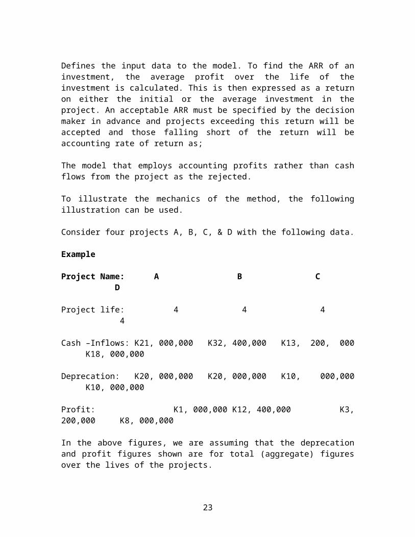
Defines the input data to the model. To find the ARR of an investment, the average profit over the life of the investment is calculated. This is then expressed as a return on either the initial or the average investment in the project. An acceptable ARR must be specified by the decision maker in advance and projects exceeding this return will be accepted and those falling short of the return will be accounting rate of return as;
The model that employs accounting profits rather than cash flows from the project as the rejected.
To illustrate the mechanics of the method, the following illustration can be used.
Consider four projects A, B, C, & D with the following data.
In the above figures, we are assuming that the deprecation and profit figures shown are for total (aggregate) figures over the lives of the projects.
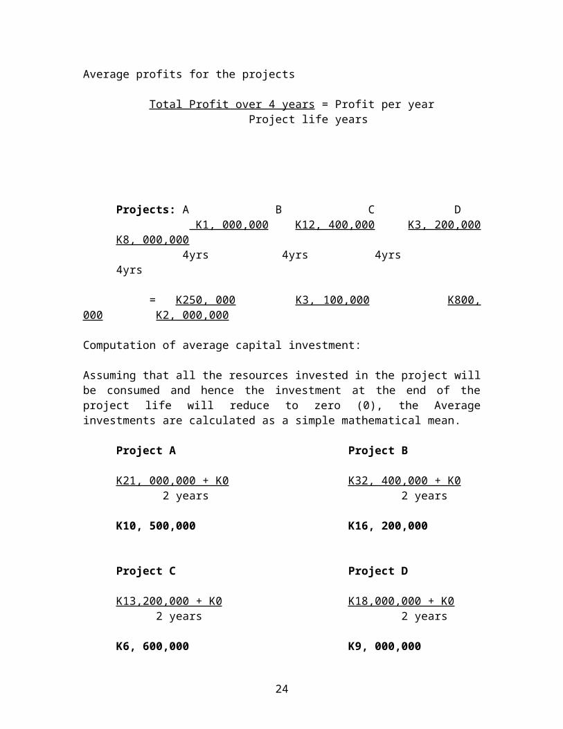
Average profits for the projects
Total Profit over 4 years = Profit per year Project life years
16
Projects: A B C D K1, 000,000 K12, 400,000 K3, 200,000 K8, 000,000
4yrs 4yrs 4yrs 4yrs
= K250, 000 K3, 100,000 K800, 000 K2, 000,000
Computation of average capital investment:
Assuming that all the resources invested in the project will be consumed and hence the investment at the end of the project life will reduce to zero (0), the Average investments are calculated as a simple mathematical mean.
Project A Project B
K21, 000,000 + K0 K32, 400,000 + K0 2 years 2 years
K10, 500,000 K16, 200,000
Project C Project D
K13,200,000 + K0 K18,000,000 + K0 2 years 2 years
K6, 600,000 K9, 000,000
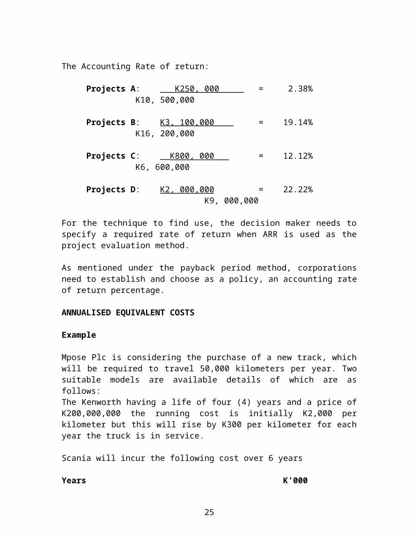
The Accounting Rate of return:
Projects A: K250, 000 = 2.38%K10, 500,000
Projects B: K3, 100,000 = 19.14%K16, 200,000
Projects C: __K800, 000 = 12.12%K6, 600,000
Projects D: K2, 000,000 = 22.22% K9, 000,000
For the technique to find use, the decision maker needs to specify a required rate of return when ARR is used as the project evaluation method.
17
As mentioned under the payback period method, corporations need to establish and choose as a policy, an accounting rate of return percentage.
ANNUALISED EQUIVALENT COSTS
Example
Mpose Plc is considering the purchase of a new track, which will be required to travel 50,000 kilometers per year. Two suitable models are available details of which are as follows:The Kenworth having a life of four (4) years and a price of K200,000,000 the running cost is initially K2,000 per kilometer but this will rise by K300 per kilometer for each year the truck is in service.
Scania will incur the following cost over 6 years
Years K’0000 350,0001 75,0002 90,0003 105,0004 120,0005 135,0006 150,000
The cost of capital for Mpose Plc is 12%
Required:
Explain which truck (between the Kenworth and the Scania) should be purchased.
Solution:
As we can see the comparison of the two projects is complicated by their unequal lines. We are going to use annualized costs to compare the two projects. Therefore the annualized cost of the Kenworth is:
Year Costs K’0000 200,0001 100,0002 115,0003 130,0004 145,000
This is determined by calculating the Net Present Value of acquiring and operating a Kenwork truck over four years and converting it an equal annual equivalent cost by dividing the Net Present Value by 3.037.
Therefore in conclusion, the Kenworth Truck is the best option with a lower annualized cost.
19
PREFERENCE FOR APPRAISAL METHOD
Investment Appraisal method
Advantages and disadvantages of Investment Appraisal Methods
PAYBACK PERIOD METHOD
Advantages
(a) It is easily understood and interpreted, especially to non-financial managers, and its implications for liquidity are clear.
(b) It can be used as preliminary project appraisal screening method, before scientific methods (discounted cash flows are applied for the appraisal process).
Disadvantages
(a) It ignores cash flows beyond the payback period and it does not take into account of the time value of money.
NET PRESENT VALUES
Advantages
(a) It takes account the timing of cash flows.(b) It takes proper account of the size and duration of projects.(c) It takes into account the greater uncertainty of later years’ cash flow by using a
higher discount rate for these years.
Disadvantages
(a) It produces a number which is less familiar to management than a rate of return.(b) It's complex in its mechanics.(c) Not easily understood by non-financial managers.
INTERNAL RATE OF RETURN
Advantages
(a) It takes into account of the timing of the cash flow.(b) It is easily compared to a given return, which project owners are looking for, in
assessing a project’s viability.
20
Disadvantages
(a) It does not take account of the size of the project, so a small project with a high return looks better than a large project with a lower return, even through the latter will contribute more to earnings.
(b) The Internal Rate of Rate (IRR) cannot evaluate properly the duration of projects. This is because IRR takes no account of what happens to the returns after they are achieved.
(c) Another potential difficulty, which may sometimes arise, is the possibility of two or more solutions to the IRR calculation. This usually happens when a project has unconventional cash flows, meaning that cash flows with negative and positive signs may come through during the life of the project.
Capital Replacement
Corporations will most times want a specific type of capital asset for a period of time which exceeds the physical life of any one individual asset, or part of an asset or part of that type. For instance, demand for the output of a particular production process may extend into the indefinite future, whereas the life of the machine required carrying out the process will be limited to a finite period.
Asset replacement may be undertaken in response to the poor physical condition of an asset or more reasonably replacement may be planned. The timetable for a planned replacement will be determined by a consideration of the costs of replacing over one time horizon rather than other.
Consider the example of a company which provides its entire sales people with a company car. The cost to the company of providing the car is made up of the initial capital cost and the annual running costs, less the resale value at the time of disposal. Data on the type of car, which our hypothetical company provides for its sales people, is given below.
K’000Initial purchases price: 50,000Annual running cost (average per year) 20,000Re-sale value if sold after: 2yrs 30,000
3yrs 25,0004yrs 15,0005yrs 5,000
21
Since the company requires the cars to extend into future, a replacement policy must be decided upon. If the company would like to minimise the overall cost of operating its fleet of cars, cars should be replaced at the point in time at which this cost is minimised. For ease of exposition we would assume that the annual operating cost is independent of the age of the car and that the data given above will remain valid indefinitely. As the annual operating cost is constant, irrespective of the replacement cycle it can be ignored for the purposes of setting the replacement policy. Therefore what needs to be considered are the purchase price of the car and the resale value.
Although, the purchase price itself is not variable the total expenditure of the company is variable as it depends on the sale of the cars, which in turns depends on the replacement cycle. The net cost of the investment in each car is given by the initial outlay less the present value of the sale proceeds.
Assuming a cost of capital of 5%, the computation would be as below.
Schedule 1
Year Resale Discount Present Purchase Net PresentValues factor (5%) values price cost K’ 000
The final column of the table shows the net present cost of owning the car over differing time periods, two years in the case of the first row, and three years for the second row etc. This cost does not of itself provide a basis for comparing the relative attractiveness of the alternative replacement cycles. In order to make such a comparison, the cost must be expressed as a net present cost per annum, which is obtained by dividing the net present cost over the relevant time period. This procedure allows the expression as an annual figure of a cost or income occurring on a regular but not annual basis.
For example taking the figures in the first row of the schedule, the K22,790,000 spent today is equivalent to an expenditure of K12,256,642 (22,790,000/1.8594) for each of the next two years at the discount rate is 5%, we would be indifferent as to which spending pattern we incurred.
It can be seen that the minimum annual equivalent cost is K10, 431,000 the cost of replacing the cars on a three-year cycle. Other things being equal the company should adopt a three-year replacement policy.
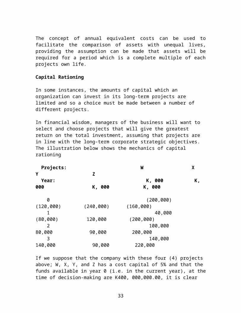
The concept of annual equivalent costs can be used to facilitate the comparison of assets with unequal lives, providing the assumption can be made that assets will be required for a period which is a complete multiple of each projects own life.
Capital Rationing
In some instances, the amounts of capital which an organization can invest in its long-term projects are limited and so a choice must be made between a number of different projects.
In financial wisdom, managers of the business will want to select and choose projects that will give the greatest return on the total investment, assuming that projects are in line with the long-term corporate strategic objectives. The illustration below shows the mechanics of capital rationing
Projects: W X Y Z Year: K, 000 K, 000 K, 000 K, 000 0 (200,000) (120,000) (240,000) (160,000) 1 40,000 (80,000) 120,000 (200,000) 2 100,000 80,000 90,000 200,000 3 140,000 140,000 90,000 220,000
If we suppose that the company with these four (4) projects above; W, X, Y, and Z has a cost capital of 5% and that the funds available in year 0 (i.e. in the current year), at the time of decision-making are K400, 000,000.00, it is clear that even if the net present values are positive the organization cannot invest in all four projects.
23
Using the profitability index technique of ranking project will be employed to rank projects.
The first step is to calculate the net present values of the projects and then express them as a percentage of the project outflow so that comparable returns are obtained.
The computation below shows the return from each project and their rankings.
Discount W X Y Z Rate @ 5% K, 000 K, 000 K, 000 K, 000 Year 0 1.000 (200,000) (120,000) (240,000) (160,000) 1 0.952 40,000 (80,000) 120,000 (120,000) 2 0.907 100,000 80,000 90,000 200,000 3 0.864 140,000 160,000 90,000 220,000 Discounted cash flows
Analysis and comment As it can be seen above, all projects have positive net present values and so they would be accepted if funds allowed.
24
With only K400, 000,000 to invest, project W would be chosen and 5/6 of project Y, assuming that the investments are divisible.
In many circumstances, divisibility of projects might not be possible, so decisions will have to be made based on net present value technique.
Capital rationing is not really a practical approach for the majority of organizations. It usually works very well if the company in question is not an Investment Company but for most of organizations providing a service or manufacturing products, this solution will not be very helpful.
Effects of Taxation on Investment Appraisal
Although in many instances we are assuming that there are no taxes in perfect financial markets, in reality taxes are usually levied on income earned from investment.
The section aims to show the effects of taxation on investment appraisal.
However, the section starts by looking at basics of discounting future cashflows, which is going to be used widely in capital investment appraisal.
Discounting Methods
Time value of money
Cash flows arising at different points in time cannot be compared directly and must be converted to a common point in time i.e. usually discounted to their present values.
Years 0 1 2 3 4
Discounting
Present value Future value
Present value (PV) is the cash equivalent now of money received/payable at some future date.
25
PV FV
Exercise
Choose between Year 0 (now) Year 5 K10,000,000,000 K5,000,000,000The discount rate is 10%Please make your decision by first discounting and then compounding.
Discounting Year 0 (now) Year 5 K10,000,000,000
K9,315,000,000 = 0.621 x K1, 500,000,000
PV = FV x 1/ (1+r) n
Compounding Year 0 (now) Year 5PV (1 + r) n = FV 10,000,000,000 × (1.1)5 = K16,105,100,000
Therefore we would choose the K10,000,000,000 now with both methods, please note that discounting is the preferred method of comparison in SFM.
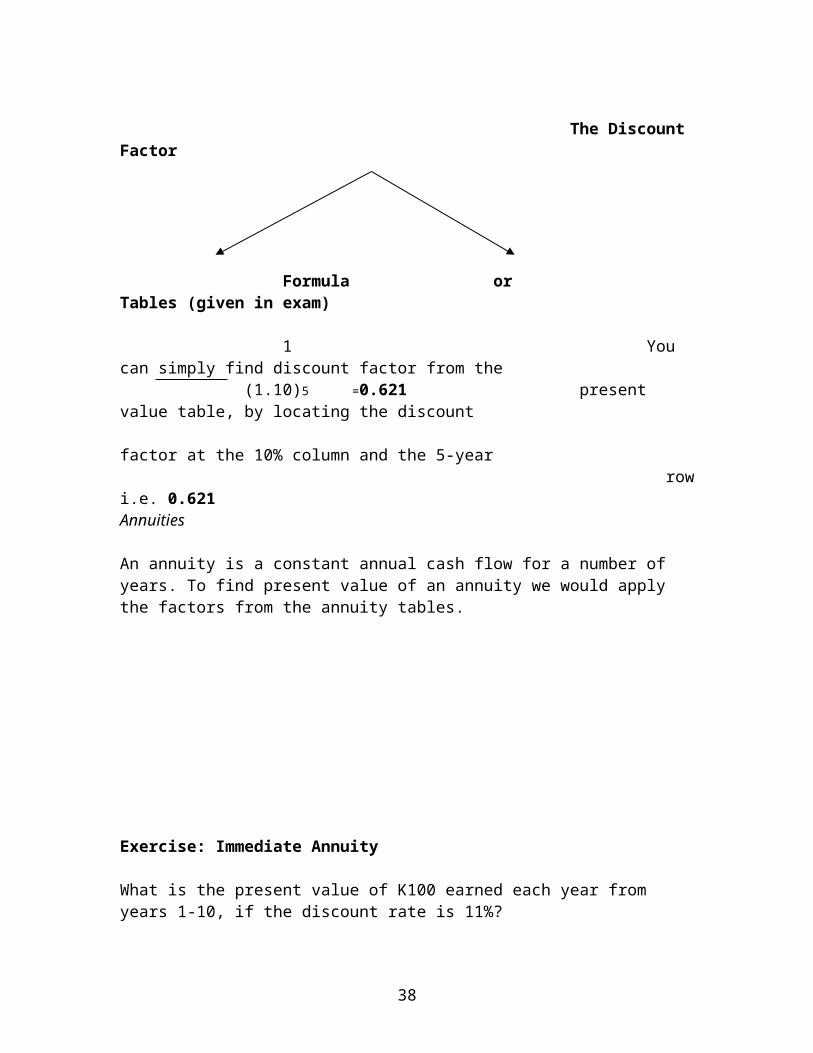
The Discount Factor
Formula or Tables (given in exam)
1 You can simply find discount factor from the (1.10)5 =0.621 present value table, by locating the discount factor at the 10% column and the 5-year row i.e. 0.621Annuities
An annuity is a constant annual cash flow for a number of years. To find present value of an annuity we would apply the factors from the annuity tables.
26
Exercise: Immediate Annuity
What is the present value of K100 earned each year from years 1-10, if the discount rate is 11%?
x
The annuity factor at year ten adds together all the present value factors for the first ten years. In fact the annuity is quite often called the cumulative present value factors. The annuity factors assume that the first cashflow occurs at the end of year one i.e. the first present value factor added in an annuity factor is for year one. Therefore when the first cash flow arises in year one you simply have to apply the annuity factor to find the present value of the annuity. An annuity which commences in year one is called 'an immediate annuity’.
Answer: PV = K100 X 5.889 = K588.9
Exercise: Deferred Annuity
What is the present value of K200 incurred each year from years 3-6 the discount rate is 5%? Answer:
The annuity factor brings all the cash flows to one year before the first cashflow arises. As the first cash flow is in year 3, all the cash flows have been brought to year 2.
To find the present value (year 0) of the annuity, which is currently valued in year two we must multiple it by the present value factor for year two.
27
1 2 3 4 5 6 7 8 9 10
(1 - 4)
0 1 2 3 4 5 6
PV
200 200 200 200
Answer = Apply the structured approached to deferred annuities:
1. Annual cash flow K200 X
2. Annuity factor for two years 1 to 4 3.546 X3. Present value factor for year 2 0.907
Present value of deferred annuity K643
Perpetuities
Perpetuity is an annual cash flow forever. It is the simplest cash flow model known to man. Goddard often implies perpetuity by simply stating, “The cash flows will occur for the foreseeable future”.
The Basic Perpetuity
PV of a perpetuity = Po = annual cash flow r
Discount rate = r = annual cash flow Po Exercise
What is the maximum amount you would pay for perpetuity of K 25,000 per annum, if the discount rate is 10%?
Answers Po = K25, 000 = K250, 000 r = 25,000 = 0.10 10 250,000
Perpetuity with Constant Growth
Perpetuity formulae also assumes that the first payment will be at the end of year one, thus they also bring the cash flows back one year.g = growth expressed as a decimal.
PV of perpetuity – Po = Cash Flow Year 0* (1+ g) r – g
Discount rate in a perpetuity – r = Cash Flow Year 0* (1 + g) Po + g
28
Exercise
What is the PV of perpetuity of K 25,000,000,000 per annum increasing at an annual rate of 5%, if the discount rate is 10% and the first payment is in year 1?
Answer:
Exercise 6: An NPV calculates with both deferred annuity and a deferred perpetuity.
The Financial Director of A plc has prepared the following schedule (excluding inflation) to enable her appraise a new project. The project’s real WACC is 10%. She wants to calculate the NPV using two different assumptions regarding the project duration. The assumptions are as follows:
a) That the real annual cash flow will be K 250,000,000,000 from year to the foreseeable future (deferred perpetuity).
b) That the real annual cash flow will be K250, 000,000,000 from year to year eighteen (deferred annuity).
Receipts – (or cost savings) X X X XPayments:Wages (X) (X) (X) (X) Materials (X) (X) (X) (X)Variable / Fixed overheads (X) (X) (X) (X)Administration / Distribution expense (X) (X) (X) (X)Capital Allowances/Tax allow dep (X) (X) (X) (X)
Taxable Profits = EBIT X X X X
Tax: (X) (X) (X) (X)
Add back: Capital Allowances X X X X
Initial outlay (X)Net Realisable Value X
Working capital (X) X
Net Cash Flows/Free Cash Flows (X) X X X X
Discount rate (X%) X X X X X
Present value (X) X X X X
Net Present Value X(X)A positive NPV is when the expected return on a project more than compensates the investor for the perceived level of (systematic) risk i.e. that the expected is greater than the required return.
Decision Rules:
Single Project:
Positive or zero NPV: Based on the estimates it appears that the project is financially viable.Negative NPV: Based on the estimates it appears that the project is not financially viable.
Mutually exclusive project (A or B): (an absolute decision not a relative decision)
Simply pick the project with the highest positive NPV.
30
The Relevant Cash Flows A key concept => include relevant / incremental cash flows in the NPV calculations.
FUTURE CASH FLOWS THAT ARISE AS A CONSEQUENCE OF THE DECICSION
1. Ignore all sunk costs incurred prior to the decision. Ignore all sunk revenues generated prior to the decision. Sunk costs are costs which have already been incurred prior to the decision. They are therefore irrelevant to the decision making process.
Exercise: R+D of K100, 000 was incurred last year.
2. Ignore all non-cash flows. E.g. depreciation.
Exercise: A company is considering investing in a project, which requires an immediate investment of K6m. This project will last for five years and at the end of the project the plant will have a scrap value of K1m. The company depreciates plant on a straight-line basis over a five-year period. What are the relevant cash flows?
Answer: Simply when you buy and a fixed asset.
3. Ignore all overheads in existence prior to the decision i.e. non-incremental cash flows. The allocation / apportionment of fixed costs already present prior to the decision are ignored.
Exercise: A manufacturing company is considering the production of a new type of widget. Each widget will take two hours to make. Fixed overheads are allocated on the basis of K1 per labour hour. If the new widgets are produced the company will have to employ an additional superior at a salary of K15, 000 per annum. The company will produce 10,000 widgets per annum. What are the relevant cash flows?
Answer: The K15,000 salary only.
Exam Focus: If you are calculating an NPV in relation to the purchase or sale of a company you should include all existing fixed costs because to the purchaser / seller they represent future cash flows will commence / cease sale.
4. Ignore interest payments and their tax effects as implicit in the discount rate. This is because if it were subtracted this would amount to double counting because the opportunity cost of capital already incorporates the cost of these funds. This simple example ignores tax relief on interest.
31
Market values Annual cash Cost of Capital Flows required
General inflation 2% Discount rate – factors Present value N.P.V
32
Two types of inflation
Specific inflation rates General inflation
Applies to all the individual cash flows items Applies to the discount rate
This is because the investors in a Project are interested in their ability to buy a basket of general goods. Not only one particular good.
The two methods
Includes the two types inflation Excludes the inflation
Money or normal Terms Real terms Discount “money” cash flows Discount “real” cash flows at money discount rate at real discount rate
Real term cash flows are Cashflows at current prices
or year zero
33
EXAM FOCUS:
When to use the money or Real method Is there one rate of inflation in the question?
No *Yes
Money / Nominal Method If the cash flows are in:
E.g. Wages 3%, Materials 4% and Real Terms Money Terms General inflation 5%
Real Methods Money Methods
* If there is one rate of inflation in the question both the real and money method will give the same answer. However it is easier to adjust one discount rate, rather than all the cash flows over a number of years. Thus the form of the cash flows defines the method to be used.
Adjusting the Discount Rate
Invariably Goddard will give you the cash flows in one form and the discount rate in the other form. So you will have to adjust the discount rate.
Cash flows in real terms Cash flows in money terms
Discount rate in money terms Discount rate in real terms
Deflate to find the real discount rate Inflate up to find money discount rate
Real discount rate to money discount rate
The fisher Equation
(1 + money rate) = (1 + real rate) x (1 + general inflation rate)
34
Exercise
If the real rate of return is 10% and general inflation is 5%, what is the money rate of return?
If the real rate of return is 8% and general inflation is 4%, what is the money rate of return?
Answer:
Money discount rate to Real discount rate
The money discount rate also sometimes called the market rate of return includes general inflation. Therefore to find the real rate of return you must deflate as follows:
Deflate:
1 + money rate = 1+ real rate 1+ general inflation
Exercise
If the money rate return is 14.4% and general inflation is 4%, what is the real rate of return?
Answer: (1.144/1.04) - 1 = 0.1 say 10%
Exercise
If the money rate of return is 13.42% and general inflation is 3%, what is the real rate of return?
Answer: (1.1342/1.03) – 1 = 0.10 say 10%
CASH FLOWS DEFINE THE METHOD ESPECIALLY WHEN THERE IS AN ANNUITY:
35
Exercise
ABC plc provides the following projected data for the next ten years excluding inflation.
0 1 2 3 – 10Net cash flows (1,700) 100 200 300
The rate of inflation is 3% and the market return is 11.24%
Calculate the present value of the cash flows over the 10-year period.
Real Method: - cash flows are in real terms; simply deflate the money discount rate to get the real rate.
Real discount rate: (1.1124/1.03) - 1 = 0.08 say 8%
Real cash flows:0 1 2 3 – 10
Net cash flows (1,700) 100 200 300Annuity factor 5.747Discount factor 1.000 0.926 0.857 0.857Present value (1,700) 93 171 1,478
NPV 42
Money Method: - calculate the money cash flows for each year and discount by the money discount rate.
“The understanding assumption that the general inflation rate is equal to the specific inflation rates for all the cash flows items is somewhat simplistic. In reality each cash
36
flow item would probably have a different specific rate of inflation, thus requiring the money method approach.”
Example:
Twincle Plc has provided and marketed camping kits for several years. The camping bags are much heavier than some of the modern camping kits being brought into the market. The company is concerned about the effect this will have on its sales. Twinkle Plc is considering investing in new technology that would enable them to provide a much lighter and more compact camping kits. The new machine will cost K500,000,000 and is expected to have a life of four (4) years with a scrap value of K20,000,000 in addition an investment of K70,000,000 in working capital will be required initially.
The following forecast annual trading account has been prepared for the project:
K’000Sales 400,000
Materials (80,000)
Labour (60,000) Variable overheads (20,000)
Depreciation (40,000)Annual profit 200,000
The company’s cost of capital is 10%. Corporation tax is charged at 30% and is payable quarterly, in the 7th and 10th months of the year in which the profit is earned and the 1st
and 4th month of the following year. A writing down allowance of 25% on a reducing balance is available on capital expenditure.
Required
Advise the management of Twinkle Plc on whether they should invest in the new technology
Your recommendation should be supported with relevant calculations. Solution
Writing down allowances
Year AssetValueK’000
30% TaxK’000
Year 1
K’000
Year 2
K’000
Year 3
K’000
Year 4
K’000
Year 5
K’000500,000
37
Yr1 25% WDA (125,000) 37,500 18,750 18,750375,000
Yr2 25% WDA (93,750) 28,125 14,063 14,063281,250
Yr3 25% WDA (70,313) 21,094 10,547 10,547 210,937
Yr4 Scrap value (20,000)Yr 4 Bal adjusted 190,937 57,281
Net Present Value of new technology investment. 141,406
Contribution = Annual Profit + Depreciation
= K200,000,000 + K40,000,000 = K240,000,000
Therefore purely on financial grounds, management of Twincle Plc should invest in the new technology, as the Net Present Value of the new technology is positive.
DIFFERENT NPV FORMATS
Exercise
DEF plc provides the following project financial data for the next 4 years, including inflation.
Year 1 Year 2 Year 3 Year 4K’000s K’000s K’000s K’000s
The rate of inflation is 3% and the real discount rate is 6.80%. Machinery cost K800, 000 life 4 years, tax allowance depreciation is at straight line and the tax rate is 30%.
Calculation of the present value of the cash flows.
Note: Only one inflation rate and cash flows are in money terms therefore use the money method. Therefore need to calculate money discount rate i.e. (1.03) x (1.068) = 1.10. i.e. 10%.
Assume that you have been appointed finance director of Breakall plc. The company is considering investing in the production of an electronic security device, with an expected market life of five years.
The pervious finance director has undertaken an analysis of the proposed project; the main features of analysis are shown below.
Proposed electronic security device project Year 0 Year 1 Year 2 Year 3 Year 4 Year 5 K’000 K’000 K’000 K’000 K’000 K’000
Investment in depreciable Fixed assets 4,500Cumulative investment inWorking capital 300 400 500 600 700 700Sales 3,500 4,900 5,320 5,740 5,320
Treatment of Leasing and Hire Purchase Transactions
Introduction
Leasing is a technique used to finance the use of an asset. It is an alternative to outright purchase, financing by using existing cash reserves or by borrowing.
The motivation for choosing leasing rather than purchasing is often tax efficiency.
A lease contract is an agreement between the owner of an asset (the lessor) and the user (the lessee) under which.
- The lessee may have use of the asset for a specified period.
- The lessee in consideration for use of the asset promises to make a series of payments/ rentals to the lessor.
- The lessor remains the legal owner of the asset during the terms of the lease.
Typically lessors would be banks or subsidiaries of subsidiaries of banks. The lessee chooses the asset and the lessor / bank purchases the asset, thus fulfilling the ownership requirements for tax purchases.
Advantages of Leasing
There are two significant reasons for a company to lease assets rather than buying outright.
1. Tax benefits2. Flexibility / cash flow3. Access to additional sources of liquidity as a result of increased debt capacity.
Tax Benefits to the Lessor
Tax saving was the original drive or motivation behind the development of the leasing market. In many countries legal ownership of a qualifying asset entitles the owner (e.g. a bank) to amortize the capital cost over the life or the lease period of the asset for tax purposes.
This gave valuable cash flows benefits to those with the taxable capacity to sketcher their tax allowances.
42
Large commercial banks usually had such tax shelter, which they could use as lessors passing on to the lessee some of the economic benefits of tax relief cash flows.
Tax Benefits to the Lessee
While the tax charges reduce the benefits of leasing, the ability of lessors to pass on capital allowance tax benefits to lessees still makes leasing attractive for entities which have no tax capacity themselves.
The circumstances in which some entities might not have tax capacity and hence can benefit from leasing would include the following;
1. In a situation where a loss making business is still creditworthy
2. Where we have start-up projects or businesses, which may not move into profits for several years such as most Biotechnology companies and start-up information technology (IT) companies.
3. For institutions which do not pay corporation tax e.g. local authorities universities and colleges.
4. In a situation where a profitable corporation, with large continuing capital expenditure and consequent large capital allowances but with low profits available as tax shelter.
FLEXIBILITY AND ENHANCE CASH FLOWS
Whilst the availability of tax allowances continues to be important the users of the leasing market rely increasingly on the advantages of cash flows and flexibility.
Lease structures can be flexible and innovative and the payment schedules can be tailored to fit the projected cash flows arising from the underlying business. For some types of assets such as aircrafts computers, containers and rail wagons, complex structures have been developed which facilitate the marketing of asset reconciling the news of the buyer and setter on their deliveries. Types of Leases
There are two main types of lease:
1. Finance leases2. Operating leases
Finance Lease
43
A finance lease transfers substantially all the risks and rewards of ownership of an asset to be leased. The rewards and risks which are to a very large extent transferred are as fellows:
The full use of assets owner it’s economic Idle capacity Breakdowns Obsolescence
The conductance below usually acts as criteria for testing a finance lease. In many laitance of a lease is going to be classified as a finance lease.
1. The present value of retails for the leased asset usually exceeds the value of the asset.
2. In a situation where the primary contact parole is somewhat equal or approximately equal to the useful economic life of the asset in question.
3. Where the retorm is margin over the lessor’s cost of funds reflecting the credit rate the contract.
The main motivation of finance lease to the lessor is to make a profit by financing the asset. As we allowed to earlier, usually such lessor we financial institutions such as bank.
Operating Lease
By definition, an operating lease is one other than a finance lease.The motivation underlying an operating lease is the leased product (asset).
The following criteria will be distinguished with operating lease. Usually in operating lease the present value of the rentals is way below the asset value.Usually the lease life (tenure) is less than the assets useful economic life. Operating leases may be a sales aid for the product manufacture/ distributor. However, if the manufacturer does not have the finance or tax capacity to act as lessor it may engage the services of a finance institution to act on its behalf.
Features of Leases
- Lease rentals.Usually equal, but can be translated to sort the lessees cash flow if value contract is large enough to justify the effort.
44
- Usually underlying interest rate Usually fixed interest rates are used smaller items for simplicity and a floating rate for large items if the lessee requires it.
- Insurance and maintenance In finance leases the lessee will be responsible for payment of such costs where as in an operating lease since the lessor is clearly the legal owner and according to the substance over form standard, the lessor will be responsible for maintenance and insurance costs payments.
- Relocation With finance leases the lessee is usually responsible for relocating the asset to the lessors’ instructions at the end of the lease contract so it can be sold.
- Sale proceedsIn most situations the major part of the sales proceeds are typically passed to the original lessee as a refund of the lease rentals.
LEASE RENTAL COMPUTATIONSEXAMPLE – TREATMENT OF LEASING AND HIRE PURCHASE TRANSACTIONS
Singa Ltd owns 20 print and computer shops in Kitwe. At present it hires its 35 photocopying machines from Rent-a-copier Ltd at an annual Rental fee of K11,200,000 each, payable monthly (assume that cashflows occur at the year end).
The rental agreement covers a 24 hour repair service which assists Singa Ltd to maintain high reputation for a quick and reliable service. Singa estimates that each machine generates K15,200,000 of contribution each year. Xero company sells photocopier machines and is trying to break into the Kitwe market and offers to sell to Singa Ltd new machines for K36,000,000 each payable on installation. Singa Ltd is considering this and has found some research that suggests that each machine stands a 0.7 chance of being unreliable. The reliability of the machines will be discovered by the end of the first year. All machines that are reliable at the end of year 1 will still be reliable at the end of year 4. If a machine proves reliable, Singa Ltd will keep it for four (4) years in total and it will generate a contribution of K16,000,000 each year after which time it will be scraped and sold for K1,200,000. If the machine proves unreliable, it will be scrapped after year one (1) and sold for K800,000. An unreliable machine is expected to generate a contribution of K10,000,000 each year.
The company’s annual cost of capital is 8%. The management of Singa Ltd consider that a time horizon of no longer than 6 years should be used when evaluating decisions on photocopiers, as beyond the date photocopier machines are likely to be outdated technology.
Required:
45
a) Prepare computations to show whether a rented or purchased machine is the financially better option.
b) Xero Company has now made an alternative introductory, once only, offer. It will buy back 30% of the machines at the end of either the first or second year if, required.
The buy – back price will be 60% of the original purchase price at the end of year 1 and 50% at the end of year 2. Singa Ltd must nominate in advance which replacement option it prefers. If Singa Ltd agrees to either of Xero company’s proposals, it would remain with the company during the life of the purchased and replaced photocopiers. Because most shops have two photocopiers available, the management of Singa Ltd has now agreed that further replaced photocopiers available, the management of Singa Ltd has now agreed that further replacements after either year 1 or year 2 would be unnecessary.
Required
Advice Singa Ltd whether or not it should accept the revised offer.
- Having prepared the calculations in (a) and (b) you now realize that the effect of taxation should have been considered. The corporation tax rate is 30%. It is payable in four quarterly installments in the seventh and tenth months of the year in which the profit is earned and in the first and fourth months of the following year. The equipment will qualify for a 25% annual reducing balance writing down allowance. Assume that the 8% cost of capital is the after tax rate for part (c).
Required:
Explain and illustrate with calculations the impact of taxation on the financial appraisal of: a rented machine a purchased reliatie machine (that is one that is kept for 4 years).
Solution:
(a) Buying a single machine: K’000 K’000
Year 0 cost 36,000 (36,000)
Reliable:
Year 1-4 (K16, 000,000 x 3.312) 52,992
Year 4 (K1, 200,000 x 0.735) 882
46
33,874 x 0.7 37,712 1,712
Unreliable
Year 1 (K10, 000,000 x 0.926) 9,260
K800, 000 x 0.926 74110,001 x 0.3 3,000
4,712Renting machine over corporate time period:
0.7 Probability of machine kept for 4 years.
= (K15, 200,000 - K11,200,000) = K4,000,000
K 4,000,000 x 0.7 x 3.312 = K9,273,600
0.3 Probability of a machine kept for 1 year:
4,000,000 x 0.3 x 0.926 = K1,111,200 Corporate figure for renting 10,384,800
Therefore the rented machine is definitely the better option:
K10,384,800 – K4,712,000= K5,672,800
1. Assume a faulty photocopier.
Year 1 replacement over year 2:
Year Cashflow Discount rate Present value (K’000) (K’000)
1 21,600 (36,000) 0.926 (13,334) (cash received a
new purchase price)
2 4,200 *1 0.857 3,600 (net benefit of new machine over 2 yrs option)
(18,000) 36,000 0.857 15,426 (saving by net replacing in
year 2)
5 1,080 * 2 0.681 735 (sale of machine)
6 (1,080) (sale income forgone)
47
(14,200) (Loss of additional years income)
2,000 0.630 (7,106)(income from renting included for companion)
* 1 0.7 x K16,000,000 = K11,200,0000.3 x K10,000,000 = K 3,000,000
K14,200,000 – K10,000,000 = K4,200,000
*2 0.7 x K1,200,000 = K840,0000.3 x K800,000 = K240,000
K1,080,000
Therefore replacement at the end of year 2 is better.
Renting over a 6 (six) year cycle:
Yr 1-6 : 35 machines x K4,000,000 x 4.623 = K647,220,000
Replacing in year 2 – assuming a full 6 year cycle for comparison
(in years 5 & 6, some machines will have to be rented, that is 35 machines x 0.7 = 24.5)
Therefore, renting still remains the better option by a small margin.
2. The amount of taxation paid will be affected by the profit earned, business expenses and the purchase of assets.
3. Machine rented
Taxation will be levied on the profit earned but the expense of renting a machine can be set against this, so the taxation calculation for renting a machine becomes (K15,200,000 – K11,200,000) x 30% = K1,200,000 per year. Half of the tax will be paid in the year in which the profit is earned and half the following year. (This will reduce the net present value over 4 years by K1,200,000 x 3.312 = K3,974,400 approximately, ignoring the time factor (lag).
4. Machine purchased
If the machine is purchased tax will still be paid on the profit earned but there will be no rented expense to set against this (increase in tax K11,200,000 x 0.3 = K3,360,000 each year for a reliable machine).
However, instead of depreciation being charged each year a capital allowance may be set against profit. The government sets the capital allowance rates. The capital allowance rate in the scenario is 25% on a reducing balance basis and the table below shows how this would be applied to a reliable machine and the final net present value of the capital allowances.
Lease rental calculations are very similar to a discounted cash flow exercise as you could have seen it early in this chapter. Rental calculation assumptions for an example, which we will work, though are summarized below. In the illustration below the tax effect the extreme case of 100% in the first year allowance and 50% tax rate is used.
Cost-Benefit Analysis
In many situations where senior managers of a business make decisions, the decisions made can either be structured or unstructured.
Structured and Unstructured Decisions
In structured decisions managers use standard procedures in an outlined manner to deal with situations in a prescribed way.
In unstructured decision-making, managers use the least pool of experience and intellect to make sound judgments, which are in the best interest of the company or organizations.
Goal Congruence and Decision Making
All decisions which are made should be consistent with the corporate objectives. We should realize at this point that business managers are leading corporations which have been established with a view to making profits.
Therefore, all decisions which the business managers make should be seen to be adding more value to the business ultimately in excess of the costs involved, than the costs involved in carrying them out.
Therefore, in whatever context we look at business decision making, business managers are going to consider the benefits against the cost of pursuing a given strategy before they embark on implementing that particular decision.
Nature of Cost- Benefit Analysis
As we have mentioned above, before a corporate strategy is implemented in a business, the managers will have need to carry out a rigorous cost benefit analysis.
Therefore, a cost-benefit analysis will involve a comprehensive comparison of the net benefits expected to accrue to an organization by pursuing a chosen strategy against the costs which are to be incurred in pursuit of the strategy.
Please note that the benefits and costs can be either quantitative and / or qualitative at the same time.
50
However, as we mentioned earlier where, the qualitative costs and benefits might be more difficult to establish due to the grey nature of the qualitative consequences of our actions. Cost- Benefit Analysis Techniques
There are a lot of techniques used to undertake cost benefit analyses.Some of the methods include the following:
Profitability/ Net Cash-Flow
Typically and usually when carrying out a cost benefit analysis, most business list the financial and quantitative revenues which the business is likely to earn against the total costs likely to be incurred in the pursuing the strategy. Scoring and Ranking
Another commonly used technique for carrying out a cost-benefits analysis is by the use of scoring and ranking of several capital investments available to the business.
Ranking and scoring is used both in situations where we are evaluating a single strategy or where we are evaluating multiple strategies so that we can eventually choose the best option out of them all.
Mechanics of Scoring and Ranking
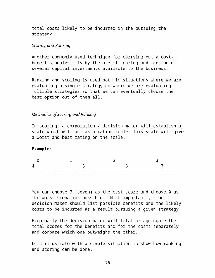
In scoring, a corporation / decision maker will establish a scale which will act as a rating scale. This scale will give a worst and best rating on the scale.
Example:
0 1 2 3 4 5 6 7
You can choose 7 (seven) as the best score and choose 0 as the worst scenarios possible. Most importantly, the decision maker should list possible benefits and the likely costs to be incurred as a result pursuing a given strategy.
Eventually the decision maker will total or aggregate the total scores for the benefits and for the costs separately and compare which one outweighs the other.
Lets illustrate with a simple situation to show how ranking and scoring can be done.
51
Assume that Chinsa Ltd has been experiencing low sales of its product, the Manex. As a result the entire management is concerned deeply and they have the following views: The Marketing Director has suggested that the company should invest heavily in the marketing activities. However, the Finance Director is a bit sceptical concerning the likely benefits of this hefty expenditure on the marketing campaign.
As a result, the CEO has requested you in your capacity as management accountant to carry out a comprehensive cost-benefit analysis. Suggested illustration
STEP 1
Set and establish a rating scale or the purpose of this illustration assuming that 1 represents the worst situation and 5 represents the best scenario.
RATING SCALE
1 2 3 4 Worst Best
STEP 2
List the likely benefits and costs of staging (mounting) up a massive marketing campaign. The likely benefits and costs would be the following: These are not exhaustive
Benefits Costs
- Good corporate image - Huge financial outlay
- Bigger client base - Expected continued advertising
- Increase profits
STEP 3
Assign weightings or ratings from the scale to each benefit and each cost
Benefits Rating
1. Good corporate image 3
2. Bigger client base 4
3. Increase profits 2
52
Total scores for benefits costs: 9
(i) Huge financial outlay 4
(ii) Expected continued advertising 4
Total scores for the costs: 8
STEP 4
Compare the total scores for benefits and the one for costs.
Benefits 9
Costs 8
Difference 1
As can be seen above, the analysis and comparison show that the benefits of staging a massive campaign will gives Chinsa Ltd more of benefits than costs.
So purely following the scoring and ranking we expect Chinsa Ltd to benefit greatly from the marketing campaign, and so the decision to invest in it should be upheld.
This is only a simplistic approach. However, in practice so many factors are likely to be taken into consideration and the management accountant will need to carryout the analysis with a great amount of help from marketing professionals and other business personal who may make work as researchers and general R&D employees with Chinsa Ltd.
It should be noted that in the above exercise, the scores represent both the qualitative and quantitative benefits, which are associated to the various benefits and costs identified by the management accountant and his team.
Post Project Completion Audit
From the onset of the chapter we have only been looking at evaluation of projects, which is only a part of the investment process.
To conclude the chapter, lets look at an equally important aspect of project evaluation and management. This is the aspect of Post-completion Audit.
The post completion audit of projects provide the mechanism whereby experience of past projects can be fed into the firm’s decision-making process as an aid to the improvement of further projects.
53
Benefits of Post –Completion Auditing
There are a number of benefits that stand out so clearly from a project post – completion audit.
The benefits can be classified in two main categories.
Type 1
Those benefits that relate to the performance to the current project i.e. the project under review.
Mechanics of Post – Completion Audit
A post – audit small team, typically professionals such as an engineer who had some involvement in the project, usually carries out completion audit.
The post – completion audit reviews all aspects of a completed project, to assess whether it lived up to initial expectations in term of revenues and costs and analyse the causes of deviations from planned results.
Its main purpose is to enable the experiences, good or bad gained during the life of one project to be made available for the benefit of future projects. The audit is thus essentially a forward-looking one as it seeks to establish lessons from the past for the future benefit of the corporation.
Type 2
The second and final category of benefits relates to the additional information concerning the choice and performance of future projects and the main benefits are given below.
It improves the quality of decision making by providing a mechanism whereby past experience can be made readily available to decision makers.
It encourages greater realism in project appraisal by providing a mechanism where past inaccuracies in forecasts are made public.
It highlights reasons for successful projects, which may be important in achieving greater benefits from future projects.
54
Chapter 2
PRICING THEORY
Learning Outcomes:
At the end of this chapter candidate Should identify and discuss market situations which influence the pricing
policy adopted by an organization Should explain and discuss the variations that influence demand of a
product or service Should be able to calculate prices using full cost and marginal cost as the
pricing base Should be able to compare the use of full costing pricing and marginal
cost pricing as planning and decision making aids Should be able to appreciate the concept of transfer pricing and its
mechanics.
55
Definition of price
Organizations operating as businesses always produce or provide tangible products or intangible services for sales to customers in order for them to pursue their primary corporate objective of enhancing shareholders wealth.
The products and services are sold at a price.
Therefore price refers to the monetary amount which corporations sale their chosen units of products/services.
Influences on Price
There are so many variations that dictate the price at which given commodities or services can be sold at.
The following are the main factors that influence price of services or products.
(a) Quality
This is an aspect of price perception. In the absence of other information, customers tend to judge quality by price. Thus a price rise may indicate improvements in quality, a price reduction may signal reduced quality.(b) Existence of intermediaries
If an organization distributes products or services to the market through independent intermediaries, such intermediaries are likely to deal with a range of suppliers and their aims concern their own profits rather than those of suppliers.
(c) Competitor Activities
In the same industries, pricing moves in unison. In others, price changes by one supplier may initiate a price war. Competition is discussed in more detail below.
(d) Inflation
In periods of inflation the organization may need to change prices to reflect increases in the prices of supplies, labour, rent and so on.
Traditional Pricing Bases
The two main traditional methods of pricing one
(i) full-cost pricing
56
(ii) marginal cost pricing
Cost plus Pricing
With full cost pricing, the sales price is determined by calculating the full cost of the product and then adding a percentage mark-up for profit, so this ensures that all costs are covered.
The full cost pricing is useful if prices have to be justified to customers.
On the other side, the full cost pricing method takes no account of the market or demand conditions.
It may also require arbitrary decisions about absorption of costs.The cost accountants may also have problems in determining the accurate profit mark-ups.
Marginal Pricing
With marginal cost pricing, a profit margin is added on to either the marginal cost of production or the marginal cost of sales.
This is sometimes called ‘mark-up’ pricing.
It draws management attention to contribution, and the effects of higher or lower sales volumes on profit.
In this way, it helps to create a better awareness of the concepts and implications of marginal costing and cost-volume profit analysis.
The marginal cost pricing is convenient if there is a readily identifiable variable cost e.g. in retail businesses.
However, again it takes no account of market or demand conditions.
In practice as you already know, pricing decisions cannot ignore fixed costs in the long term.
Example
Muti Ltd has begun to produce a new product, product X, for which the following cost estimates have been.
KDirect materials 27,000
Direct labour: 4 hours at K5,000 per hour 20,000
57
Variable production overheadsMachining, ½ hour at K6,000 per hour 3,000
50,000
Production fixed overheads are budgeted at K300,000 per month and because of the shortage of available machining capacity, the company will be restricted to 10,000 hours of machine time per month. The absorption rate will be a direct labour rate, however, and budgeted direct labour hours are 25,000 per month. It is estimated that the company could obtain a minimum contribution of K10,000 per machine hour on producing items other than product X.
The Direct Cost estimates are not certain as to material usage rates and direct labour productivity, and it is recognized that the estimates of direct materials and direct labour costs may be subject to an error of + 15%.
Machine time estimates are similarly subject to an error of + 10%.
The company wishes to make a profit of 20% of full production cost from product X. What should the full cost based price be?
The following solutions have been developed based on four (4) assumptions.
(a) Exclude machine time opportunity costs:
Ignore possible costing errors K
Direct materials 27,000
Direct labour (4 hours) 20,000
Variable production overheads 3,000
Fixed productionOverhead (K300,000,000 = K12,000 per
25,000 48,000direct labour hour
Full production cost 98,000
Profit mark-up (20%) 19,600
Selling price per unit of product X 117,600
(b) Include machine time opportunity costs:
58
Ignore possible costing errors. K
Full production cost is in (a) 98,000
Opportunity cost of machine time(Contribution forgone (½hr x K10,000) 5,000
Adjusted full cost 103,000
Profit mark-up (20%) 20,600
123,600
(c) Exclude machine time opportunity costs but make full allowance for possible under-estimates of costs.
K KDirect materials 27,000Direct labour 20,000
47,000
Possible error (15%) 7,050 54,050
Variable production Overheads 3,000
3,000Fixed productionOverheads (4 hrs x K12,000) 48,000
Possible error (labour time) (15%) 72,000 55,200
Potential full production cost 112,550
Profit mark-up (20%) 22,510
135,060
(d) Include machine time opportunity costs and make a full allowance for possible under-estimates of cost.
KPotential full production cost as in (c) 112,550
59
Opportunity cost of machine time(Potential contribution forgone)(½hr x K10,000 x 110%) 5,500
Profit mark-up (20%) 23,610
Selling price per unit of product X 141,660
Full Cost Versus Marginal Cost Pricing
The most important and common criticism of full cost pricing is that it fails to recognize that since sale demand may be determined by sales price, there will be a profit – maximization combination of price and demand.
A full cost based approach to pricing will be most unlikely, except by coincidence or luck to arrive at the profit-maximising price. In contrast a marginal costing approach to looking at costs and prices would be more likely to help with identifying a profit–maximising price.
Example
Luangwa Ltd has budgeted to make 50,000 units of its product, the Luan.
The variable cost of a Luan is K5,000 and annual fixed costs are expected to be K150,000,000.
The Finance Director of Luangwa Ltd suggested that a profit margin of 25% on full cost should be charged for every product sold.
The Marketing Director has challenged the wisdom of this suggestion, and has produced the following estimates of sales demand for the Luan.
Price per unit Demand K Units 9,000 42,00010,000 38,00011,000 35,00012,000 32,00013,000 27,000
Required
(a) Calculate the profit for the year if a full cost price is charged.
(b) Calculate the profit-maximising price.
60
Assume in both (a) and (b) that 50,000 units of the Luan are produced regardless of sales volume.
Solution
(a) (i) The full cost per unit is K5,000 variable cost plus K150,000,000 = K3,000\unit 50,000 units
hence i.e. K8,000 (K5,000 + K3,000) in total.
A 25% mark-up on this cost gives a selling price of K10,000 per unit so that sales demand would be 38,000 units. (production is given as 50,000 units).
(ii) Profit (absorption costing)
K 000 K000
Sales 380,000
Costs of production (50,000 units)
Variable (50,000 x K5,000) 250,000
Fixed (50,000 x K3,000) 150,000
400,000
Less increase in stocks(12,000 units x 8) (96,000)
Cost of sales 304,000
Profit 76,000
(i) Profit using marginal costing instead of absorption costing so that fixed overhead costs are written off in the period they occur, it would be as follows (the 38,000 unit demand level is chosen for comparison purposes).
KContribution (38,000 x K(10,000 – 5,000) 190,000 Fixed costs 150,000
Profit 40,000
61
Since the company go on indefinitely producing an output volume in excess of sales volume, this profit figure is more indicate of the profitability of the Luan in the longer term.
(b) A profit-maximising price is one which gives the greatest net (relevant) cash flow, which in this case is the contribution-maximising price.
Price Unit Contribution Demand Amount K K units K 9,000 4,000 42,000 168,00010,000 5,000 38,000 190,00011,000 6,000 35,000 210,00012,000 7,000 32,000 224,00013,000 8,000 27,000 216,000
The profit maximizing price is K12,000 with annual sales demand of 32,000 units.
This example shows that a cost based price is unlikely to be the profit – maximizing price, and that a marginal costing approach, calculating the total contribution at a variety of different selling prices, will be more helpful for establishing what the profit – maximizing price ought to be.
Activity Based Pricing (ABP)
Activity based costing provides an opportunity for organizations that use cost-based pricing to gain a greater understanding of their costs and so correct pricing anomalies that derive from the distorted view given by conventional volume-related costing.
Under the ABC approach, overheads are allocated to products on the basis of the activities that caused them to be incurred, rather than according to some arbitrary base like labour hours. The implication for pricing is that the full cost on which prices are based may be radically different if ABC is used.
Example
ABP Ltd makes two products, X and Y with the following cost patterns.
Product Product X Y K K
Direct materials 27,000 24,000
Direct labour at K5,000/hr 20,000 25,000
62
Variable productionOverheads at K6,000 Per hour 3,000 6,000
50,000 55,000
Production fixed overheads total K300,000,000 per month and these are absorbed on the basis of direct labour hours. Budgeted direct labour hours are 25,000 hours per month. However, the company has carried out an analysis of its production support activities and found that its fixed costs actually vary in accordance with non volume-related factors.
Product Product Total CostActivity Cost driver X Y K 000Set-ups Production runs 30 20 40,000
Material Production runs 30 20 150,000
Inspection Inspections 880 3,520 110,000300,000
Budgeted production is 1,250 units of product X and 4000 units of product Y.
Required:
Given that the company wished to make a profit of 20% on full production cost, calculate the prices that should be charged for products X and Y using the following.
(a) Full cost pricing(b) Activity based cost pricing
Solution
(a) The full cost and mark-up will be calculated as follows:
Product Product X Y
K K
Variable costs 50,000 55,000
Fixed productionOverheads
63
*K300,000,000\25,000 = 12,000\hr) 48,000 60,000
98,000 115,000
Profit mark-up (20%) 19,600 23,000
Selling price 117,600 138,000
(b) Using activity based costing, overheads will be allocated on the basis of cost drivers.
The results in (b) are radically different from those in (a). On this basis it appears that the company has previously been making a huge loss on every unit of product X sold for K117,600. If the market will not accept a price increase, it may be worth considering leasing production of product X entirely. It also appears that there is scope for a
64
reduction in the price of product Y and this would certainly be worthwhile if demand for the product is elastic.
Target Pricing
Target costing is a pro-active cost control system. The target cost is calculated by deducting the target profit from a predetermined selling price based on customer’s views. Techniques such as value analysis are used to change production methods and or reduce expected costs so that the target is met.
Target cost is an estimate of a product cost which is derived by subtracting a desired profit margin from a competitive market price.
Target cost management has been defined as a system that is effective in managing costs in new product design and development stages. It has also been viewed as allowing the production cost of a proposed product to be identified so that when sold it generates the desired profit level.
Target cost management has also been viewed as playing a useful role in enabling an enterprise to set and support the attainment of cost levels to effectively reflect its planned financial performance.
What appears to be evident is that there are almost as many misconceptions of target costing as there are companies deploying the approach and there are probably many companies engaging in various aspects of target cost management without referring to the term.
Managerial Thinking to Support Target Costing and Pricing
Target costing requires managers to change the way they think about the relationship between cost, price and profit.
(a) The traditional approach is to develop a product, determine the expected standard production cost of that product and then set a selling price\probably based on cost) with a resulting profit or loss. Costs are controlled through variance analysis at monthly intervals.
(b) The target costing approach is to develop a product concept and the primary specifications for performance and design and then to determine the price customers would be willing to pay for that concept.
The desired profit margin is deducted from the price leaving a figure that represents total cost. This is the target cost and the product cost and the product must be capable of being produced for this amount otherwise the product will not be manufactured.
65
During the products life the target cost will constantly be reduced so that the price can fall. Continuous cost reduction techniques must therefore be employed.
The Target Costing Process
Step 1
Analyse the internal environment to ascertain what customers require and what competitors are producing. Determine the product concept, the price customers will be willing to pay and thus the target cost.
Step 2
Split the total target cost into broad cost categories such as development, marketing, manufacturing and so on. Split up the manufacturing target cost per unit across the different functional areas of the product. Design the product so that each functional product area can be made within the target cost. If a functional product area cannot be made within the target costs, then a cost gap exists between the currently achievable cost and the target for the other areas must be reduced, or the product redesigned or scrapped. The product should be developed in an atmosphere of continuous improvement using value engineering techniques and close collaboration with suppliers, to enhance the product (in terms of service, quality, durability and so on) and reduce costs. Step 3
Once it is decided that it is feasible to meet the total target costs, detailed cost sheets will be prepared and processes formalized.
Final Commentary on Target Pricing
Target pricing therefore will involve pegging a pricing for a product or service which will well cover the targeted cost of manufacturing a product or providing a service.
Life Cycle Pricing
Life cycle costing assists in the planning and control of a product’s life cycle by monitoring spending and commitments to spend during a product’s life cycle.
Life cycle costs are incurred for products and services from their design stage through development to market launch production and sales, and their eventual withdrawal from the market.
Traditional management accounting systems in general only report costs at the physical production stage of the life cycle and do not accumulate costs over the entire life cycle. They assess a product’s or project’s profitability on a periodic basis. Life cycle costing, on the other hand, considers a product’s\project’s entire life.
66
Life cycle costing tracks and accumulates actual costs and removes attributable costs to each product or project over the entire product\project life cycle.
The total profitability of any given products\project can therefore be determined.
Traditional management accounting systems usually total all non-production costs and record them as a period expense.
Using life cycle costing, such costs are traced to individual products over complete life cycles.
(a) The total of these costs for each individual product can therefore be reported and compared with revenues generated in the future.
(b) The visibility of such costs is increased.(c) Individual product profitability can be more fully understood by attributing all
costs to products.(d) As a consequence, more accurate feedback information is available on the
organisation’s success or failure in developing products. In today’s competitive environment were the ability to produce new and updated versions of products is paramount to the survival of an organization, this information is vital.
The strong force which supports life cycle costing is that generally for organizations operating within the manufacturing technology environment, its found that approximately 90% of a product’s life cycle cost is determined by decisions made early within the cycle at the design stage.
Life cycle costing is therefore particularly suited to such organizations and products, monitoring spending and commitments to spend during the early stages of a product’s life cycle.
Life cycle pricing therefore involves pricing a product at a rate which covers the costs which are anticipated over the entire life cycle of the product in question.
Remember the product life cycle you learnt in management.
67
Illustration of product life cycle
Sales revenue
introduction growth maturity decline sales
Time
Other Pricing Methods
Order Pricing
A special order is a one-off revenue earning opportunity.
These may arise in the following situations.
(i) When a business has a regular source of income but also has some spare capacity allowing it to take on extra work if demanded.
For example Nkwazi Breweries might have a capacity of 500,000 barrels per month but only producing and selling 300,000 barrels per month.
It could therefore consider special orders to use up some of its spare capacity.
(ii) When a business has no regular source of income and relies exclusively on its ability to respond to demand.
A building firm is a typical example as are many types of subcontractors.
In the case of (i) pricing for special orders need therefore take account of unavoidable fixed cost because any firm like in the case of (i) is not attempting to cover its longer-term running costs in its prices for its regular product or services.
68
However, in the case of (ii) where the special order is the only source of income, all costs incidental to the special order and the fixed unavoidable cost should be incorporated in the special order pricing.Minimum Pricing
A minimum price is that which would have to be charged so as to cover the following two groups of cost.
(i) The incremental costs of producing and selling the product/service.
(ii) The opportunity costs of the resources consumed in making and selling the product/service.
A minimum price would leave the business no better or worse off than if it did not sell the item.
Two important points to understand here about a minimum price are as below:
(a) It is based on ‘relevant costs’
Relevant costs are incremental costs plus the opportunity costs of making and selling the product or providing a service.
(b) It is unlikely that a minimum price would actually be charged because if it were it would not provide the business with any incremental profit.
If there are no scarce resources, and a company has spare capacity, the minimum price of a product would be an amount which equals the incremental cost of making it.
If there are scarce resources and a company makes more than one product, minimum prices would include an allowance for the opportunity cost of using the scarce resources to make and sell the product.
Market Penetration Pricing
Penetration pricing is a policy of low prices when a product is first launched in order to obtain sufficient penetration in to the market.
A penetration policy may be ideal in the following cases:
(a) When the firm wishes to discourage new entrants into the market.
(b) When the firm wishes to shorten the initial period of the product’s life cycle in order to enter the growth and maturity stages as quickly as possible.
(c) When demand is highly elastic and so would respond well to low prices.
69
(d) When there are significant economies of scale to be achieved from a high volume of output.
Market Skimming Pricing
Price skimming involves charging high prices when a product is first launched in order to maximize short – term profitability. Initially there is heavy spending on advertising and sales promotion to obtain sales. As the product moves into the later stages of its life cycle, progressively lower prices are charged. The profitable ‘cream’ is thus skimmed off in the early stages until sales can only be sustained at lower prices.
The aim of market skimming prices is to gain high unit profits early in the product’s life. High unit prices makes it more likely that competitors will enter the market, that is if lower prices were to be charged.
So market skimming pricing would be appropriate in the following cases.
(a) When the product is new and different, so that customers are prepared to pay high prices so as to be one up on other people who do not own it.
(b) When high prices in the early stages of a product’s life might generate high initial cash flows. A firm with liquidity problems may prefer market-skimming for this reason.
(c) Where products may have a short-life cycle, and so need to recover their development costs and make a profit relatively quickly.
Examples of products to which market skimming pricing policy could be applied would include latest versions of products such as
(i) Calculator(ii) Video recorders(iii) Desktop computers and other technology based products.
Differential Pricing
The use of differential pricing means that the same product can be sold at different prices to different customers.
This can be very difficult to implement in practice because it relies for success, on the continued existence of certain market conditions.
We can exercise differential pricing on the following cases:
(i) By market segment e.g. services such as cinemas and hair dressing are often available at lower prices to juveniles and old age pensioners.
70
(ii) By product version e.g. many car models have ‘Add on’ extras which enable one brand to appeal to a wider cross-section of customers.
(iii) By place e.g. theatre seats are usually sold according to their location so that patrons pay different prices for the same performance according to the seat type they occupy.
(iv) By time e.g. this is perhaps the most popular type of differentiating pricing.
E.g. Celtel charges less for its air time or credit in off peak period and vice versa.
Price differentiation can only successfully be implemented if the market can be well segmented and there is little chance of arbitrage or chance of a black market developing (which would allow those in the lower priced segment or bracket resale to those in the higher priced segment or bracket).
Example: Transferring Goods at market price
A company has two profit centres; A and B. Centre A sells half of its output on the open market and transfers the other half to B. Costs and external revenues in a period are as follows.
A B TotalK’000 K’000 K’000
External sales 8,000 24,000 32,000Costs of production 12,000 10,000 22,000Company profit 10,000
Required
What are the consequences of setting a transfer price at market price?
If the transfer price is at market price, A would be happy to sell the output to B for K8, 000, 000, which is what A would get by selling it externally.
(a) A earns the same profit on transfers as on external sales. B must pay a commercial price for transferred goods.
(b) A will be indifferent about selling externally or transferring goods to B because the profit is the same on both types of transaction. B can therefore ask for and obtain as many units as it wants from A.
Adjusted Market Price
Internal transfers in practice are often cheaper than external sales, with savings in selling and administration costs, bad debt risks and possibly transported/delivery costs. It would seem reasonable for the buying division to expect a discount on the external market price.
If profit centres are established, however, and unit variable costs and sales price are constant, there are two possibilities.
(a) Where the supplying division has spare capacity the ideal transfer price will simply be the standard variable cost of production.
(b) When there is a scarce production resource, the ideal transfer price will be the variable cost of production plus the contribution forgone by using the scarce resource instead of putting it to its most profitable alternative use.
Cost-based approaches to transfer pricing
Cost-based approaches to transfer pricing are often used in practice, because there is often no external market for the product that is being transferred or because, although there is an external market, it is an imperfect one because there is only limited external demand.
Transfer prices based on full cost
Under this approach the full standard cost (including fixed overheads absorbed) that is incurred by the supplying division in making the product is charged to the receiving division. If a full cost plus approach is used, a profit margin is also included in this transfer price.
A company has 2 profit centers, A and B. Centre A can only sell half of its maximum output externally because of limited demand. It transfers the other half of its output to B which also faces limited demand. Costs and revenues in a period are as follows.
A B TotalK’000 K’000 K’000
External sales 8,000 24,000 32,000
72
Costs of production in the division 12,000 10,000 22,000(Loss)/Profit (4,000) 14,000 10,000
If the transfer price is at full cost, A in our example would have ‘sales’ to B of K6,000,000 (i.e. half of its total costs of production). This would be a cost to B, as follows.
The transfer sales of A are self-cancelling with the transfer costs of B so that total profits are unaffected. The transfer price simply spreads the total profit of K10,000,000 between A and B. Division A makes no profit on its work and using this method, would prefer to sell its output on the open market if it could.
Transfer prices based on full cost plus
If the transfers are at cost plus a margin of, say, 25%, A’s sales to B would be K7,500,000.
A B K’000 K’000 K’000 K’000
Open market sales 8,000 24,000 Transfer sales 7,500 -
Compared to a transfer price at cost, A gains some profit at the expense of B. However, A makes a bigger profit on external sales in this case because the profit mark-up of 25%
73
is less than the profit mark-up on open market sales, which is (K8,000,000 – K6,000,000)/ K6,000,000 = 33%. The transfer price does not give A fair revenue or charge B a reasonable cost, and so their profit performance is distorted. It would seem to give A an incentive to sell more goods externally and transfer less to B. This may or may not be in the best interests of the company as a whole.
Division A’s total costs of K12,000,000 will include an element of fixed costs. Half of division A’s total costs are transferred to division B. However from the point of view of division B the cost is entirely variable.
Suppose that the cost per unit to A is K15,000 and that this includes a fixed element of K6,000, while division B’s own costs are K25,000 per unit, including a fixed element of K10,000. The total variable cost is really K9,000 + K15,000 = K24,000 but from division B’s point of view the variable cost is K15,000 + K15,000 = K30,000. This means that division B will be unwilling to sell the final product for less than K30,000 whereas any price above K24,000 would make a contribution.
Changes in price levels
Changes in price levels are a common scenario in the operations of company. The change in the price levels may be due to external or internal factors. A price change may be necessitated by a general increase in the cost of production or high levels of demand for the company’s products or services.
It is important to relate the price changes to both production costs and selling price of the product or service.
A price change can also arise when a company is introducing a new product asit is common for a number of prices to be considered. Since price level changesrepresent decision-making under conditions of risk and uncertainty, it is important to analyse the expected outcome for each price level.
Any price change is bound to affect the demand and therefore the variable costs giving varying possible outcomes.
Example
Mwine manufacturing company has come up with a new soap product, Buta detergent. From the preliminary studies the following analysis has been made;
Selling price Selling price K 8,500 K 10,0
Outcomes Demand Probability Demand Probability Probable 40,000 0.6 50,000 0.1 Less Probable 30,000 0.1 20,000 0.5 Most Probable 60,000 0.3 30,000 0.4
74
Outcomes At Selling Price K 8,500
Demand Contribution Fixed Cost Net Price Expected Value
From the outcome it is evident that chosing the selling price of K 8500 gives a higher expected value, even though the difference is not so significant.
In practice however other factors may be considered. Furthermore it will not be an easy task to come up with an accurate estimate of future demand and the probable outcomes.
Transfer Pricing Theory
This is the price at which goods and services are transferred between different units of the same company. If those business units are located within different countries, the term international transfer pricing is used.
Transfer prices are a way of promoting divisional autonomy, ideally without prejudicing the measurement of divisional performance or discouraging overall corporate
75
maximization. The management accountant therefore has to devise a transfer pricing method that meets the following criteria:
Equity (provides a fair measure of divisional performance)
Neutrality (avoids the distortion of business decision making)
Administrative simplicity
The transfer price should provide an “artificial” selling price that enables the transferring division to earn a return for its efforts and the receiving division to incur a cost for benefits received, and should be set at a level that enables profit centers to be measured ‘commercially”. This means that the transfer price should be a fair commercial price.
Transfer pricing with a constant unit variable costs and sales price:
An ideal transfer price should reflect the opportunity cost.
Where a perfect external market exists and unit variable costs and sales are constant, the opportunity cost of transfer will be one or other of the following
External market price
External market price less savings in selling costs.
Example
A company has two profit centers, A and B. Center A sells half of its output on the open market and transfers half to B. Costs and external revenues in a period are as follows.
A B TotalK K K
External sales 8,000,000 24,000,000 32,000,000
Costs of production 12,000,000 10,000,000 (22,000,000)
Company profits 10,000,000
Required
What are the consequences of setting a transfer price at the market price?
Transfer prices based on variable cost
76
A variable cost approach entails charging the variable cost that has been incurred by the supplying division to the receiving division. As above, we shall suppose that A’s cost per unit is K15,000, of which K6,000 is fixed and K9,000 variable.
A BK’000 K’000 K’000 K’000
Market sales 8,000 24,000 Transfer sales at variable cost 3,600 ___ -(9,000/15,000 x 6,000) 11,600 24,000Transfer costs 3,600Own variable costs 7,200 6,000Own fixed costs 4,800 4,000Total costs and transfers 12,000 13,600(Loss)/Profit (400) 10,400
The problem is that with a transfer price at variable cost the supplying division does not cover its fixed costs.
Transfer prices based on opportunity costs
It has been suggested that transfer prices can be set using the following rule.
Transfer price per unit = standard variable cost in the producing division plus the opportunity cost to the organization of supplying the unit internally.
The opportunity cost will be one of the following.
(a) The maximum contribution foregone by the supplying division in transferring internally rather than selling externally
(b) The contribution foregone by not using the same facilities in the producing division for their next best alternative use
(a) If there is no external market for the item being transferred, and no alternative uses for the division’s facilities, the transfer price = standard variable cost of production
(b) If there is an external market for the item being transferred and no alternative use for the facilities, the transfer price = the market price.
Transfer pricing when unit variable costs and sales prices are not constant
When unit variable costs and/or unit selling prices are not constant there will be a profit-maximising level of output and the ideal transfer price will only be found by careful analysis and sensible negotiation.
77
(a) The starting point should be to establish the output and sales quantities that will optimise the profits of the company or group as a whole.
(b) The next step is to establish the transfer price at which both profit centers, the supply division and the buying division, would maximize their profits at this company-optimising output level.
(c) There may be a range of prices within which both profit centers can agree on the output level that would maximize their individual profits and the profits of the company as a whole. Any price within the range would then be ‘ideal’.
Problems in transfer pricing
(a) If transfer prices are set at full cost, the transferring division makes no profit.
(b) If full cost plus is used the problem is how to set the margin at a level that all parties perceive as being fair.
(c) If variable cost is used the transferring division does not cover its fixed costs but two-part prices (the variable cost transfer price plus a fixed annual fee) might be used to overcome this.
(d) Transfer prices based on standard cost are fairer than transfer prices based on actual costs because if actual costs are used the transferring division has no incentive to control its costs: it can pass on its inefficiencies to the receiving division.
(e) On the other hand, standards may become out of date so it is advisable to have an agreement to revise them periodically.
Negotiated transfer prices
When authority is decentralized to the extent that divisional managers negotiate to transfer prices with each other, the agreed price may be finalized from a mixture of accounting arithmetic, politics and compromise.
Inter-departmental disputes about transfer prices are likely to arise and these may need the intervention of head office to settle the problem.
(a) Head office imposition. Head office management may impose a price that maximizes the profit of the company as a whole.
(b) On the other hand, head office management might restrict its intervention to the task of keeping negotiations in progress until a transfer price is eventually settled.
78
Where negotiation is necessary there should be an understanding of the risk/return profile. Tomkins suggests the following methodology, which head office can apply when mediating in disputes.
(a) Identifying the outer bounds of the transfer price. In other words, at what transfer price does the buying division end up earning the entire group profit, and at what transfer price does the selling division earn the entire group profit?
(b) Variability. At each transfer price, compare each division’s expected profits and the variability of the profits.
(c) Incorporate risk attitudes in a fair transfer price, so that the profit-share between divisions takes the riskiness of the project into consideration.
International transfer prices
When firms transfer goods and services not only internally, but also internationally, the transfer price mechanism allows them to move value from one country to another without actually engaging in trade. Bearing in mind the difficulty discussed above of establishing the level at which a transfer price should be set, we may say that a ‘low’ price effectively moves value into the receiving country, while a ‘high’ one moves it into the transferring country.
Using transfer prices
This ability to decide in which country value (and particularly profit) is created is extremely useful.
(a) It can be used to manage taxation;
(i) Profit can be minimized in states with high profit taxes(ii) Selling prices can be minimized in states with high levels of irrecoverable
VAT (and similar taxes)(iii) The value imported into countries with high tariff levels can be minimized
(b) It can be used to move profits to the home country from states with restrictions on repatriation of profits or on currency exchange.
(c) It can be used strategically
(i) It can disguise the attractiveness of an operation to competitors by reducing profits.
(ii) It can enable a low-price strategy aimed at driving out competition without arousing the suspicions of the local tax authorities by declaring a
79
very low level of profit. However, this course of action is likely to lead to accusations of dumping.
Centrally determined transfer prices and strategy
These considerations produce pressure for multinational companies to set their transfer prices centrally. There are, however, other important strategic considerations relating to this approach.
(a) Autonomy. Centrally determined transfer prices can seriously affect the ability of national managers to influence the performance of their divisions. This can affect their overall motivation, encourage them to seek ways around the restrictions imposed and make it more difficult to assess their overall performance.
(b) Transaction cost economics. Transaction cost theory is dealt with in Paper 5 but it is also relevant to Paper 6. In terms of transaction cost economics, a centrally determined, non-market based transfer price makes an implicit assumption that the hierarchy solution is the best one. However, there may not have been any actual consideration of the market alternative. A resource or competence based approach to strategy would immediately challenge this and call for detailed consideration of the benefit of a market based approach. The crucial question is whether the business should actually be operating any given national subsidiary at all, whether its services should be bought in.
The Eccles matrix
R J Eccles suggests that the method of setting transfer prices should reflect the organisation’s degree of diversification and its degree of vertical integration.
(a) Where both diversification and integration are low, as, for example, in the relationship between two shops in a retail chain, a transfer price may not even be required, but if it is, it can be set collaboratively.
(b) Where diversification is low, but vertical integration is high, as in the relationship between two different stages of product assembly, co-operation is important, so the transfer price should be negotiated: it should probably be set at full cost so that resource allocation is appropriate and the supplying division’s costs are covered.
(c) Where diversification is high and integration is low, as in the now unfashionable diversified conglomerate, transfers are likely to be uncommon and should be at market price, as is the rest of each subsidiary’s trade.
Nevertheless, where diversification and integration are both high, as may be the case when there is extensive trade along a supply chain combined with similarly extensive market-based exchanges, once again, the transfer price should be set collaboratively.
80
Chapter 3COST ANALYSIS
Learning outcomes
After studying this chapter, a student would be able to understand the behaviour and reduction of costs in both traditional and advanced manufacturing environments. The chapter in particular looks at:
the learning curve in theory and practice the experience curve ‘traditional’ cost-reduction methods focused cost-reduction programmes value-added and non-value-added activities zero-base budgeting systems (PPBS) value analysis (VA) value engineering (VE) functional analysis target costs and costing cost tables life cycle costing
81
life cycle budgeting
INTRODUCTION
The well-known economists’ short and long-run cost curves show a general tendency for costs to decline as the volume of output increases. The long-run average cost curve reflects changes in plant capacity and processes; the short-run average cost curve reflects the change in unit production cost that arises through the operation of a given set of production factors over a limited range of outputs. Thus the short-run curves show that costs may increase in the short term, as excessive demands are placed on a particular plant, illustrating the economist’s ‘law of diminishing marginal returns’ in respect of short-run costs. These increases can be avoided by moving onto the long-run curves by increasing capacity through a further investment in fixed assets, which enables a firm to continue to benefit from reducing unit cost as total output increases. Assuming the time scale allows investment, it is a firmly-established tenet of economics that unit cost will decline as output increases. The reasons for this decline, referred to as economics of scale.
The economists’ diagram is a static representation of costs, given a particular set of materials, technologies etc. It is accepted in economics that not all firms will enjoy the same level of success in actually attaining the minimum cost levels possible for a particular negotiated bulk discounts with suppliers, but firms can experience differing levels of success in such negotiations. A skilful negotiator is in a position to obtain a cost advantage for his company if competitors employ less adept buyers. Similarly, the economist’s cost curves are premised on the use of the most cost effective production processes and materials. A company which identifies the availability of and successfully implements or uses, a new cost effective production process or material will thus gain a cost advantage over its competitors. This advantage will only be temporary if the competitors quickly follow suit, but may be permanent if it allows the innovator to cut prices and gain market share at the expense of slower moving competitors, who may be driven out of business as a result. It will always be beneficial for a firm to be able to produce goods at a lower cost than the competition and firms will therefore strive constantly to achieve cost reduction.
The CIMA Terminology defines cost reduction as:
‘the reduction in unit cost of goods or services without impairing suitability for the use intended’. As the economists cost curves indicate, a reduction in unit cost can be achieved simply by increasing the volume of production. In the present context, it is more appropriate to think of cost reduction as the reduction in unit cost at all levels of output, i.e. to view it as an attempt to move the long-run average cost curve down and back towards the origin. In reality, many firms have a less than precise understanding of the detailed cost curves relating to their industry. Nevertheless, they will usually have an understanding and a
82
bench-mark against which to measure their success in cost reduction. If companies are able to reduce total cost, whilst maintaining current output, cost reduction will certainly have been achieved. If output is increased, but there is also an increase in cost, the position is less clear. If the increase is proportionally greater than the increase in cost and assuming that functionality of the product has been maintained, cost reduction in terms of the terminology definition will have taken place. However, this may not reflect a great achievement on the party of the company: the cost reduction may simply have arisen as an inevitable consequence of the economies of scale, which the increased production has facilitated. If an expanding company is to make genuine achievements in the area of cost reduction, in the sense outlined above, it may be able to distinguish between those saving which occur merely as a consequence of increased volume, and those which arise through management action. Management needs to be aware of both types of savings in view of the importance for budgeting and decision making of a clear understanding of how costs will vary with changing output level.
One of the economies of scale enjoyed by firms as output increases may be attributable to the ‘learning curve’. This phenomenon, known as the ‘cost reduction curve’, is discussed below.
THE LEARNING CURVE
THE NATURE OF THE LEARNING CURVE
According to learning curve:
‘The mathematical expression of the phenomenon that, when complex and labour-intensive procedures are repeated, unit labour times tend to decrease at a constant rate. The learning curve models mathematically this reduction in unit production time’.
The recognition of the so-called learning curve phenomenon stems from the experience of aircraft manufacturers, such as Boeing, during World War II. They observed that the time taken to assemble an individual aircraft declined as the number of aircrafts assembled: as workers gained experience of the process, their proficiency, and hence speed of working increased. The ‘learning’ gained on the assembly of one plane was translated into the faster assembly of the next. (This is phenomenon to which any reader who has never put together a number of flat-pack items of furniture will readily relate). The actual time taken by the assembly workers was monitored, as it was discovered that the rate at which the learning took place was not random, but was rather predictable. It was found that cumulative average time per unit decreased by a fixed percentage each time the cumulative production doubled. In the aircraft industry, the percentage by which the cumulative average time per unit declined was typically 80 percent. For other industries, other rates may be appropriate. Further, the unit of measurement may sensibly be taken as a batch of product, rather than as an individual unit. This does not, of course, affect the underlying principle.
83
Let us take as an example a learning rate of 90 percent. In this case, if the first batch of a product is produced in 100 hours, the cumulative average time taken to produce two batches (a doubling of the cumulative production) would be 90 hours giving a total production time of 20 x 90 = 180 hours. The actual time taken to produce the second batch (the batch being the unit of measure in this case) will thus be 80 hours the cumulative total time taken to produce two batches – 80 hours – less the time taken to produce the first batch-100 hours. As a doubling of cumulative production is required, in order to observe the benefit of learning in the form of reduced average labour hours per unit of cumulative production, it will be appreciated that the effect of the learning rates on labour time will become much less significant as production increases. The figure below shows this.
FIGURE 3.1: CUMULATIVE DATA GRAPHS
Cumulative data graph
Log ofcum.averagetime perbatch,hours
Log of no. of batches (or units)
In constructing table 1, it was assumed that we already knew the learning rate, which applied to this particular situation. However, it must be appreciated that, in the real world, this rate can only be established by observation. Records must be kept of the number of units/batches produced and the associated time taken, in order to construct the equivalent of Table 1 (although it is likely that fewer observations would actually be taken). It is then the job of the engineer or accountant to deduce the learning rate from these observations, which will require the specification of an equation to fit the data. For
84
example, the observation in Table 1 is plotted in Figure 3.1, and can be described by the equation:
Yx = aXb Eqn 1Where:
(i) Yx is the cumulative average time per unit/ batch taken to produce a Cumulative numbers of units/ batches X;
(ii) ‘a is the time required to produce the first unit/batch;
(iii) X is the cumulative number of units/batches under consideration
(iv) The exponent ‘b’ is the index of learning.
This is known as the cumulative average-time learning model.
Consideration of the formula in equation 1 shows that it is the value of ‘b’ which determines the shape of the learning curve. If no learning effect were present, the time taken to produce any unit would be equal to the time required to produce the first unit, i.e.
Yx = a
And the learning ‘curve’ would be a straight line, as all units would take the same timer to produce. Consideration of equation 1 shows that this can only be true if Xb=1. And, as x, by definition, is greater than 1 for all except the first unit, b must equal 0 if Xb is to equal 1(X0=1), i.e. no learning is present.
Any value of b greater than 0 would result in Yx increasing as x increased, meaning that the average time taken to produce units was increasing rather than decreasing, i.e negative learning was taking place. Thus, if a positive learning effect is present, b must be less than zero, i.e. b must be a negative number.
If we assume that a positive learning effect is present, at one unit/batch of output;
Y1=a
Consider now the effect of doubling the output, i.e. X = 2, then
Y2=Y1x learning rateand; Y2 = a x learning rate
But from Equation1, Y2=a2b, therefore;
A x learning rate = a2bLearning rate =2bLog (learning rate)=b (log2)
85
Therefore b=log (learning rate) Log2
So, for a 90% learning rate, b= log 0.9 log 2
All numbers less than zero have a negative logarithm, while all numbers greater than zero have a positive logarithm. Therefore, when learning is taking place, b must be negative.
The Terminology gives the mathematical description of the learning curve as:
Y= a Xβ
Where: (i) Y is the average time taken per unit/batch to produce a cumulative number
of units/batches(ii) ‘a’ is the time required to produce the first unit;(iii) x is the cumulative number of units to be produced; (iv) ‘B’ is the coefficient of learning.
The B in the Terminology is thus equal to-b in Equation 1, and the two formulae are mathematically equivalent (students should note that, in examinations, yet another variant of Equation 1 is often given, i.e. the learning curve is expressed as).
a Y = xn
In this case, n is equal to both B as defined in the Terminology and –b as in Equation 1.
Let us apply the formula in Equation 1 to the operations of the manufacturer whose data is recorded in Table 1 and whose learning rate is 90 per cent, by checking the cumulative average time which we would expect will be necessary to produce 64 batches:
Yx = aXb Eqn (1)
b = log 0.9 = -0.1520 log 2
Yx = aX-0.1520
Yx =100 x 64 -0.1520
Yx = 53.14
Which agrees with Table 1 above.
86
In the example above, ‘b’ equals –0.1520, giving learning rate of 0.90. The learning rate can take any value, but only values of less than one imply that learning is taking place. Learning rates greater than 1 imply that the time taken per unit/batch is increasing as production increases, a value of exactly 1 would indicate that the time taken per unit/batch was not changing at all, and values less than one mean that the time taken per unit/batch is declining as production increases.
Equation 1 is not normally used to check earlier calculations in the way that we have just done, but is rather used to assess the time which will be required for an output level which does not represent a doubling of the cumulative production total, and thus cannot be determined by simply creating a table such as the one used earlier. For example, let us assume that the manufacturer above has the opportunity to bid for a contract to produce 10 batches of his product, and wishes to estimate the time it will take to complete the contract, in order to help set the tender price. If the cumulative total production of his product to date is 32 batches equation 1 can be employed to calculate the cumulative average time per batch to produce 42 batches – the 32 already produced plus the 10 under consideration:
Yx = aXb Yx = 100 x 42 -0.1520
Yx =100 x 0.5666Yx = 56.66
i.e. the average time per batch to produce 42 batches is 56.66 hours, giving a total production time of 56.66 x 42 = 2,380 hours.
Inspection of Table 1 above reveals that the average time per batch to produce 32 batches is 59.05 hours, with a total production time of 1,890 hours. The total time taken to produce the 10 batches under consideration will thus be 2,380 – 1,890 = 490 hours, i.e. an average time of 49 hours for each of the batches 33 to 42. This may be compared with the average of (3,401 – 1,890)/32 = 47.20 hours indicated by Table 1 for the next doubling of a full 32 batches from 33 to 64. obviously, if the current level of production does not lie on a table such as Table 1, that particular average time, and the corresponding cumulative hours to date, will need to be calculated from the same formula.
USES OF THE LEARNING CURVE
(i) In circumstances where the learning curve is likely to operate i.e. in complex assembly operations, knowledge of the rate of learning can help in price setting.
(ii) When setting budgets, the effects of the learning curve should be taken into account. The learning curve has been found to be particularly useful in determining the likely costs to be incurred in fulfilling government contracts. This provides a rational basis for price negotiation and cost control.
A number of points about learning curves must be stressed:
87
- Learning curves chart the reduction in time per unit as experience is gained; they do not measure a reduction in cost per se. However, if hourly wages are constant, the labour cost per unit will decline as a result of the learning curve phenomenon.
- In addition to direct labour costs, only those costs which are directly related to direct labour time, i.e. any overheads which vary directly with those hours, can be expected to decline as a result of the learning curve.
- Learning is likely to be greatest in complex assembly environments, of which aircraft assembly is a prime example. If labour is working in a machine-paced environment, there is no significant opportunity to alter the rate of working and thus the learning phenomenon in terms of direct labour time cannot exist. However, the experience which plant managers gain in scheduling work in such an environment may result in a reduction in the direct labour hours required for a given level of production.
- The learning rate, which is a function of workers’ learning, is not something which can be positively fostered as a cost –reduction technique.
THE EXPERIENCE CURVE
It has been stressed that the learning curve was derived from observations of the reduction in direct labour time taken to complete successive repetitive but complex assembly tasks that have frequently been determined by fitting curves to total tasks. However, learning rates have frequently been determined by fitting curves to total cost per unit data. For example, Depuy (1993) used this method to ascertain for the US government the learning rate achieved by defence contractors. The purpose in gathering this data was to help in price negotiations with the contractors. The total cost data employed was expressed in constant dollar terms, and thus was not distorted by changing price levels. The slope of the learning curves derived ranged from 0.718 to 1.021, with a mean of 0.858. This data suggest that defence contractors typically enjoy a reduction of 14 per cent of average unit cost on each doubling of output. The strict application of the learning curve phenomenon is seen in the area of direct labour, and it is arguable that, in using unit cost data, the result outlined above actually reflects the so-called ‘experience curve’, rather than the learning curve as strictly defined. The ‘experience curve’ extends the learning curve approach to areas other than direct labour. Rather than relating indirectly to cost via time, an experience curve relates directly to cost, and is a function which shows how total cost per unit declines as output increases. Total cost in experience curves includes all overhead types – production, marketing and distribution – and thus cost reductions arising from factors such as factory size, production, technology, substitution of materials and design modifications are reflected in an experience curve.
Experience curve, like learning curves, can be regarded as statements of what will happen in practice. This could be considered to be a western approach. An alternative approach, adopted by the Japanese, is that these curves should be taken as an expression of what is desirable, and hence what should be striven for. The improvement –oriented Japanese typically aim actively to foster a 67 per cent learning curve, as against the 80 per cent curve more usually found in the West.
88
Moses (1991) has pointed out that the accounting policies adopted by companies can have a significant impact on learning rates derived from experience curves, and so the results must be treated with caution.
Cost Reduction
INTRODUCTION
An appreciation of the relationship between cost and volume is important in many business decisions, of which pricing is a prime example. When average total unit cost is measured against volume, a measurement is being made which allows a long-run average cost curve to be graphed. Where learning or experience curves are used to predict future costs, there is an implicit assumption that the experience of the past is helpful in predicting the future. This may well be the case, but it provides no operational guidance to management as to how cost reductions are to be achieved in the future. Indeed, knowing that the learning curve has led to cost reductions in the past could give rise to a dangerous complacency on management’s part, if it is assumed that, as long as volume increases, savings will continue to be made in the future even if no positive action is undertaken to secure them.
Organisations which set targets for cost reduction, and have systems in place to help the accomplishment of those targets, are more likely to achieve cost reductions, then organisations which do not adopt such a systematic approach. Obviously, the scope for cost reduction will be dependent on the type of cost under consideration, and the time scale involved.
‘Traditional’ Cost-Reduction Programmes
‘Traditional’ cost reduction programmes have been characterized as ‘a collection of crash programs that focus on cutting costs by reducing payrolls and eliminating jobs’ (shields and Young (1992). It is suggested that such programmes are typically triggered in reaction to an immediate threat, such as poor performance, loss of contracts, or price reductions – in other words, traditional programmes are often reactions to events rather than anticipations of them. There is some evidence to suggest that these programmes do not meet their objective. Fisher (1991) cites two surveys on this point: half the managers in the first survey (representing corporations accounting for 26 per cent of US GNP) said that the cost –cutting or restructuring programmes had failed to meet their objectives; the second survey of managers from 1,005 corporations found that more than half the corporations had failed to meet their cost – reduction targets.
Market pressure to reduce costs could lead companies to attempt a ‘blanket’ approach to cost cutting, particularly for overheads. For example, in an attempt to reduce costs by, say 5 per cent, a company may take a decision to cut all departmental budgets by the same 5 per cent. This might achieve some short –term savings but it is likely to be at the expense of the long-term health of the organisation. A blanket cut will affect all activities equally, which means that some areas which were of value to customers will inevitably suffer. In a commercial organisation, this will lead to some loss of business, which may lead to an
89
increase in unit cost, as fixed overheads (albeit reduced by 5 per cent in our example) are spread over a smaller number of units sold.
A successful cost reduction programme will seek to reduce the unit cost of the good or service at all volumes of output. This can be achieved by reducing either direct costs or overhead costs, and ideally reducing both, but without destroying value to the customer. The blanket cut strategy to achieving this is ineffective in the long term. Firms must adopt approaches which enable them to pinpoint and realize specific opportunities for cost savings.
Examination of Current Activities
The starting point for cost reduction programmes often is the examination of existing activities. Any organisation can be seen as a collection of activities designed to lead to a desired result. In carrying out these activities to meet the short-term operating plan, a company may currently be incurring higher costs than are strictly necessary, i.e. the company’s consumption of resources is excessive. Examination of current operations may reveal that this over –consumption of resources arises from one or a combination of the following three reasons:
1. Over – resourced activities 2. Inefficiently managed activities 3. Unnecessary (non-value added/diversionary) activities Each of these reasons will be looked at in turn and the effectiveness of a blanket cut in resources to achieve cost reduction in these circumstances will be considered.
Over-Resourced Activities
An activity is over –resourced when the same objective could be achieved with less resource consumption. For example, in a production department, shop floor manning levels may have remained within the same processes. The current position may be one in which a separate operative is assigned to each machine. However, if the process requires very little human intervention, it may be perfectly possible for machines to be physically grouped in such a way as to allow a reduction in staffing levels, so that one person may be able to oversee two, three, four or even more machines, without any loss of machine efficiency.
A blanket cut in resources may provide the spur to such reorganizations, although the industrial relations implications of reduced staffing levels may make attainment of the most cost- effective arrangement difficult to achieve.
Inefficiently Managed Activities
Activities are inefficiently managed when current standards of achievement are not being attained. Loss of material through pilferage, excessive overtime working necessitated by
90
poor production scheduling and excessive time spent on rework through failure to identify problems at the earliest opportunity would all provide example which highlight variances from standards. Regular monitoring will identify these deficiencies and should lead to their elimination. However, a blanket cut in resources may provide an additional impetus to improvement.
Value Added and Non-Value Added Activities
The concept of a value- added activity revolves around the customer. Value will be added when an activity results in an addition to a product or service which they ultimate consider to be valuable, and which is therefore some thing for which they are willing to pay. A non- value added activity is thus any activity which does not provide value to an end user. Non- value added activities often arise as a direct consequence of, and are sustained, by, a company’s existing policies and organisational structure. It is only possible to eliminate such non- value added activities if changes are made to the current policies and structure. For example, a company may have a department devoted to dealing with customer complaints, and the rectification of problems which arise during a products warranty period. This department’s activities will increase the costs of the business, but are non- value added as far as the consumer is concerned. The existence of a warranty is useful to the end user, and adds value as a result, as it provides a level of insurance, and hence peace of mind. However, not only is a claim under a warranty and value added for the customer, in as much as it provides law enhancement to product it self, but the customer is also invaluably put to some trouble in actually making such a claim. Problems with products are thus both a cost to company and an inconvenience to the costumer. Self evidently, as the reliability of a product increase, warranty claims will decline. The inherent reliability of a product will be the function of the product design, the quality of the materials used and the manufacturing process; non of these activities are under the control of warranty department management.
A blanket cut in resources, applied to the warranty department along with all other departments, would be unlikely in its self, to result in the action which would improve the overall product reliability. If the warranty department is not currently over-resourced, and is efficiently managed, a cut in its resources is highly likely to reduce the level of service that it can provide to customers- customers who, by definition, are already unhappy with the service which the company has provided in selling them a faulty product. Delays in rectifying faults are likely to lead to a further loss of consumer goodwill, and hence damage the competitive position of the company even more. To control the resources consumed by overhead department effectively, it is essential to understand:
(a) why such departments exist;(b) the services they provide;(c) there relationship to other areas of the business.
In other words, it is necessary to adopt a cross-functional attitude to the examination of the business processes. Activity-based cost management adopts this approach, as we shall see in the next chapter.
91
Other approaches to overhead cost reduction, which eliminates the disadvantages of blanket approach to cost, cutting, is zero-base (priority-base) budgeting, to which we now turn.
Zero-Base Budgeting
Like all budgeting techniques, zero-base budgeting (ZBB) is designed to be used in setting levels of future expenditure. As all cost reduction techniques must, by definition, relate to the reduction of future costs (past costs being sunk) it follows that cost-reduction programs and budgeting procedures are in inextricably entwined. The Terminology defines zero-base/priority-base budgeting as:
‘A method of budgeting which requires each cost element to be specifically justified, as though the activities to which the budget relates were being undertaken for the first time. Without approval, the budget allowance is zero’.
The reference to ‘funds available’ is particularly pertinent in public sector organisations, where funds are determined by tax revenues and government grants and allocations, i.e. the income of the organisation, is exogenously set. The aim of the fundholder is to achieve the best service levels possible within the given budget.
In traditional budgeting, existing expenditure levels form the base line for discussions about future expenditure. Implicit in the traditional approach is an assumption and acceptance that current expenditure is adding value to the customer, and the focus of its attention is simply the justification of any proposed increases in the expenditure – it therefore adopts an incremental philosophy to budgeting. The rejection of this base line as a starting point is what gives zero-base budgeting its name. An incremental approach is most likely to be applied to discretionary costs, as it is these costs, which is thus likely to lead to the most radical changes in discretionary areas. Nevertheless, the approach requires all activities to be justified and prioritised before the decision to devote resources to particular ones is taken.
All activities are subjected to the most basic scrutiny and answers sought to such fundamental questions as:
(a) Should the activity be undertaken at all?(b) If the company undertakes, how much should be done and how well should it be
done (for example, should an economy or a de-luxe service level be provided)?(c) How should the activity be performed- in house or sub –contracted? (d) How much would the various alternative levels of service and provision cost?
In order to answer these questions, all existing and potential organisational activities must be described and evaluated in a series of ‘decision packages’, giving the following four-step process to a ZBB exercise:
92
1. Determine the activities, which are to be used as the object of decision packages – the provision of home support for the elderly or provision of catering facilities for the work force, for example - and identify the manger responsible for each activity.
2. Request the managers identified in (1) above to prepare a number of alternative decision packages normally requested: one which sets out what could be delivered 80 per cent of the current level and one for an enhanced level of funding, (e.g. 120 per cent of the current level).
3. Rank the decision packages in order of their contribution towards the organisation’s objectives.
4. Analyse alternatives, and go for these those with the greatest cost benefit in term of the objectives;
5. Systematically implement the selected alternatives.
Some explanation of these steps is necessary. Effectiveness can be judged only against predetermined benchmarks set by the organisation. Yet the activities performed by public –sector and not-for-profit organisations are often difficult to measure in a tangible way, and can take several years to be measurable, while required to overcome these difficulties. Many programmes will also have multiple results, and a choice must usually be made regarding the relative weights attached to them. Further, there will often be questions regarding the legitimacy of casual relationships when measuring these results: particular outcomes could be brought about by the actions of more than one programme, given the nature of public –sector and not for profit organisations and their objectives.
On a more positive note, one feature of PPBS that should be particularly beneficial is that managers making budget requests are expected to be able to state clearly what would happen if their requests were cut by, say 10 per cent. Thus the director of leisure services in a local authority should be in a position to say that such a cut would reduce the hours that a swimming pool could open, for example, or require that the grass in public parks be cut every ten days instead of once a week. This feature of PPBS is, in its result, somewhat similar to ZBB, since different levels of service are associated with each level of requested funding.
The interest in PPBS probably owes much to an increasing public demand for accountability by public and other not-for-profit organisations: taxpayers appear to have become dissatisfied with the performance of central and local government agencies; and donors to charitable causes have expressed concern about the proportion of contributed funds devoted to administrative expenses. PPBS specifies goals clearly, and allows people to see where their, money is going and, eventually, to see whether or not it was spent effectively.
Exercise: The Alpha Group
93
The Alpha Sufferers Group is a national charity offering support to sufferers and funding medical research. You have been invited to attend a trustees’ meeting at which the following report on this year’s performance and next year’s annual budget will be discussed. No further supporting information is provided for the trustees. The trustees have used an incremental approach to determine the budget.
The treasurer has heard of ‘programme – planning budgeting system’ and wonders if it would be useful in their not-for profit-organisation.
Criticise the current method of budgeting and explain the application (give specific examples) and possible advantages of PPBS to such an organisation.
19X3 19X4
Budget Actual Budget Actual Income Subscription 20,000 18,000 20,000Donations received
160,000 200,000 220,000
Fund – raising 500,000 440,000 484,000680,000 658,000 724,000
666,000 735,000 788,000Excess of income over expenditure 14,000 77,000 (64,000)Timing and Focus of Cost – Reduction Programmes
It is axiomatic that, in searching for cost savings, the greatest effort should be expended in investigating those costs which provide the greatest opportunities for savings. However, these opportunities are related to time. As Berliner and Brimson (1988) have pointed out, and as Figure 3.3 illustrates, up to 90 per cent of a product’s costs will be fairly limited for an existing range of products. Nevertheless, cost reduction programmes have tended to focus on current production costs, despite the evidence that the ability to influence cost is greatest at the planning, research and development stages.
94
Programmes which focus on reducing cost at these early stages after the greatest opportunities for success in the medium to long term, although their impact in the short term may be small. The most successful cost-reduction programmes at the conceptual and design stage are those which have a strong market focus. Rather than aiming to meet the manufacturer’s own internal specification at least cost, they involve a thorough examination of customer requirements, in order that these can be satisfied at least cost.
One technique of cost reduction, which recognises the importance of concentrating effort on the design and conceptual stage, is ‘value analysis’ (also known as ‘value engineering’), which is discussed below.
COST CONTROL
Cost control involves management action undertaken to effectively mange thecosts of running an under-taking. A good cost control system should be able to bring about control over the costs of the entity.
In order to come up with an effective cost control system, a methodical approach is required. To this effect, the following approach can be used:
Stage 1 Target Setting
Any cost control system requires targets to be fixed for costs. The target so setmust, however, be revised continuously in order to keep them in line with the current cost efficiencies.
Stage 2 Measure the Actual Results
There must be an effective and up-to-date system to measure actual results. The actual results should be measured as frequently as possible.
Stage 3 Comparison between Targets and Actuals
This stage involves comparing the targets with the actuals. It is important that any differences between the targets and the actuals are analysed into sufficient details. Reasons for the differences must be identified.
Stage 4 Identifying the causes for the differences
Stage 5 Action to prevent variances
Having identified the reasons for the variances, it is important that necessaryaction is taken to void the recurrence of the variances.
95
From the above, it is notable that in order to have an effective cost controlsystem, the appropriate targets must be set, an effective comparison systemmust be in place and the results must be analysed sufficiently.
The common types of cost control systems are the budgeting control systemsand the standard costing systems.
Value Analysis
The disruption of normal supply lines to American manufacturers in World War II necessitated a search for substitute materials and alternative designs. Value analysis (VA) evolved as a result of these experiences. The approach was championed by General Electric of America, and is associated with two employees in particular: Harry Erlicher and Lawrence Miles. Erlicher, who was vice-president of purchasing, observed that many of the enforced changes which the war had brought about had actually improved performance and/or reduced cost. At the ceassation of hostilities, therefore, he decided to maintain and institutionalise the search for substitute materials and methods. In 1947, the task of putting this into practice was assigned to Miles, who was then a staff engineer. The result was value analysis, which combines a number of pre-existing techniques with its own particular procedural approach. General Electric adopted the approach as a company standard, and it was subsequently taken up by other companies and organisations, including the American military. In 1954, the Navy Bureau of Ships, aided by Miles set up a VA programme, in which the term (VE) rather than ‘value engineering programme was established in 1956 by the Army Ordnance corps, and the Air Force began investigating the technique in 1961, having been stimulated by the success of suppliers, such as General Electric, in its operation. Indeed, the US Defence Department became so convinced of the benefits to be gained from VE that Secretary of Defence McNamara referred to it in 1962 as a key element in the drive to reduce defence costs. The Armed Service Procurement Regulations made the use of VE mandatory, and defined it as:
‘ A systematic effort directed at analysing the functional requirement of the Department of Defence systems, equipment, facilities and supplies for the purpose of achieving essential functions at the lowest total cost, consistent with the needed performance, reliability and maintainability’.
This definition can be seen to be consistent with the CIMA Terminology definition of ‘value analysis’, which is taken from BS 3138:
Although the term ‘value engineering’ is used by purists to refer to the applicant of the ideas of value analysis, Miles used the two terms synonymously, and they will be treated as such throughout the remainder of this chapter.
The technique is regarded primarily as a means of achieving cost reduction, and can be applied to existing or new products at any stage of the life cycle. However, as we noted earlier, the scope for achieving cost savings is greater during the pre-production phases,
96
and it is therefore at these early stages that the application of VA offers the greatest cost reduction opportunities.
Figure 3.2
_ _ _ _ _ _ _ _ _ _ _ _ _ _ A
Minimum amount Cost content that must be spent attributable to to make the product the product
A - CB Work added by Unnecessary design Value and specification analysis features zoneC
Total cost Work added by MethodAssociated with inefficient methods studythe product of manufacture zone(under absorptionsystem) A - D
D Overhead carried Production because man or control machine or both are zone
97
In the search for cost reduction, the concept of minimum cost is a dynamic, not a static one. It alters with changes in design, volume, materials and technology etc. Figure 3.2, adapted from Gage (1967), provides a useful description of the focus of a number of cost-reduction techniques.
There is a strong inter-relationship between the zones in Figure 3.2, particularly when new products are being considered. The minimum amount which must be spent to produce a new product cannot be determined until the design and specification of the product has been determined – the value analysis zone – and until the method of manufacture. A simultaneous consideration of the two (‘simultaneous engineering’) is likely to lead to lower –cost solutions rather than a sequential consideration (‘over-the-wall engineering’). Value analysis seeks to facilitate this simultaneous approach. It aims to ensure that the product brief is tightly specified, in terms of the functionality required, and that design and production engineers not only understand the brief, but contribute simultaneously to it. A team approach is thus crucial to the Value Analysis philosophy. The Value Analysis team must ponder the following six basic questions when applying Value Analysis to any product or service:
1. What is it?2. What does it do?3. What is it worth?4. What does it cost?5. What else would work?6. What does that cost?
Alternatives that reduce the design complexity of a product, and lower its bulk or weight and/or the number and variety of parts required in its manufacture, are frequently associated with reduced cost. The accountant clearly has a role to play in determining the cost of these alternatives. Miles (1972) has suggested that;
... Meaningful costs may be obtained from a variety of sources or from a combination of sources:
But since, in many instances of good value work, materials, products and processes will be utilised in different ways, really meaningful costs often must be worked up for the job’(emphasis added).
Miles suggests that cost estimates do not need to be of a high degree of accuracy, particularly in the initial stages of Value Analysis, when the aim is to identify fruitful avenues for investigation, rather than to make final decisions.
98
Nevertheless, when final decisions are being made, accuracy will obviously be important. The ability to make accurate estimates in respect of products and processes of which the firm may have no direct experience is therefore a valuable one.
The first two of the six questions above relate to the functions of the product or service. ‘Functional requirements’ were mentioned in the definition of Value Engineering above, and we have talked of ‘functionality’ in the context of the requirements of the product brief. The concept of product or service function is thus a key element in the Value Analysis approach, and it’s to this concept that we now turn.
Functional Analysis
Functional analysis (FA) is a systematic approach to the examination of the specified purpose of a product or service. In functional analysis, the cost object is the function of the product or service itself. Functional analysis views all products as bundles of services potential for customers, so that the cost object is represented by this intangible service potential. The focus is thus very different from traditional accounting, which often has a physical product as its cost object.
As an example of functional analysis, let us consider a domestic telephone. This has as its major function the facilitation of communication between individuals who are physically separated. When expressed in this way, it is clear that the competition for sales of domestic telephones is represented not only by other handset manufacturers, but also by suppliers of any means of long distance communication – telex, fax, the postal system etc.
Functional analysis can be applied in a number of ways. It may be used as an aid to cost reduction, and as a means of improving products, by adding new features in a cost effective manner. In value analysis, for example, a clear understanding of the function of a product or service is essential, in order to determine how that functions can be supplied to the customer in the most cost –effective way. Functional analysis can also be used to assist in the determination of expected selling prices, as consumers may be expected to pay particular prices for particular functions. In this context, functional analysis can be seen to underpin target costing, which we will discuss in the next section of this chapter. Yoshikawa et al (1993) suggest that the six basic questions listed in Value Analysis section can be answered by following the nine basic steps set out below:
1. choose the object of analysis, such as product, service or overhead area;2. select the members of the team;3. gather information;4. define the functions of the object;5. draw a functional family tree;6. evaluate the functions;7. suggest alternatives, and compare these with the target cost choose the alternatives
(for manufacturing etc);8. review the actual results.
99
The range of options for consideration under step 7 may relate to a whole range of functions, or may relate to alternative ways of satisfying a particular set of functions that will not yet have been fixed. Value analysis allows the team to consider a range of functional combinations, together with their associated costs and to compare these with the prices customers are likely to be willing to pay for the alternative combinations, in order that the optimal set can be selected. On the other hand, when a company is analysing a defence contract, the required functions are likely to be very closely specified, so that the analysis will probably be confined to financial evaluation of the differing means of satisfying the given functional ends.
VE undertaken at the research and development phase is something referred to as ‘zero look VE’, that undertaken in the trial production phase as ‘first look VE’, and that in the trial production phase as ‘second look VE’. Second look VE can be used when design changes are being made to existing products. These descriptions illustrate the iterative nature of cost-reduction techniques.
VALUE ENGINEERING
As discussed above is also called value analysis. Definition: This is a systematic interdisciplinary examination of factorsaffecting the cost of a product or service in order to devise means of achievingthe specified purpose at the required standard of quality and reliability at targetcost.Aim of Value EngineeringThe aim of value engineering is to achieve the assigned target cost by
i. Identifying improved product designs that reduce the product’s cost without sacri-ficing functionality and
ii. Eliminating unnecessary functions that increase the product’s costs and for which customers are not prepared to pay extra for.
Value engineering requires the use of functional analysis. This process involves decom-posing the product into its many elements or attributes.
ExampleIn the case of automobiles, functions might consist of STYLE, COMFORT, SPEED, RELIABILITY, QUALITY, COLOUR etc (KATO 1993). A price or value for each element is determined which reflects the amount the customer is prepared to pay. To obtain this information companies normally conduct surveys and interviews with customers. The total of the values for each function gives the estimated selling price from which the target profit is deducted to derive the target cost. The cost of each function of product is compared with the benefits perceived by customers. If the cost of the function exceeds the benefit to the customer, then the function should be either eliminated, modified to reduce its cost or enhanced in terms of its perceived value so that its value exceed its cost. Also by focusing on the product’s functions, the design team will often
100
consider components that perform the same function in other products thus increasing the possibility of using standard components and reducing costs, e.g. Nokia has the same charger for each type or mode phone manufactured.
Activity based costing
INTRODUCTION
A core accounting activity is the analysis of costs. Costing systems accumulate costs by broad classifications – material, labour, power etc. - and these costs are then further analysed by assigning them to cost objects. A cost object is defined as anything for which a separate measure of costs is desired, and thus the range of possible cost object is vast – from individual product to department, customer, service, brand or project. The costing system will routinely collect information about some but by no means all, possible cost objects. Costing information is needed for a variety of reasons:
(i) Stock valuation for financial accounting purposes;(ii) Cost control and performance evaluation;(iii) Decision-making, e.g. product pricing, drop a product, make or buy etc.
The selection of cost objects for the routine collection of information has implications for each of the above three purposes. It is common to find departments, cost centres and products as cost objects in costing systems.
Considerable dissatisfaction has been expressed at the information provided by ‘traditional’ costing systems for purposes (ii) and (iii), and particular attention has been directed to finding the ‘true’ cost of producing a product to supply information for (iii). However, it is important to emphasise that the concept of a ‘product’ as a cost object needs amplification.
Example
Cost management is as important for the automobile industry in the 1990s as what quality control was in the 1970 and 1980s. (extract from & corporate annual report)
Required
(i) Explain the meaning of the ‘cost management’, which is sometimes known as cost management information.
(ii) Discuss why it might be considered important in today’s world.
(iii) Discuss how a management accountant might use investment appraisal techniques to analyse customers in order to aid cost management.
101
Solution
(i) Cost management or cost management information are rather vague and general phrases used by different people to mean lightly different things. A general definition of cost management information is;
The application of management accounting concepts, methods of data collection, analysis and presentation, in order to provide the information required to enable costs to be planned, monitored and controlled.
(ii) It is certainly important today for all organisations to satisfy their customers by meeting their needs precisely. This involves providing the right product at the right place at the right time and at the right cost.
During the 1980s, Japanese car companies such as Toyota paid a great deal of attention to quality – consider, for example, the development of the Lexus model targeted at the USA market.
The management accountant has a role to play in this area, and target costing and life cycle costing are particularly helpful in driving costs down.
(iii) A management accountant can use discounted cashflow or payback to evaluate the work of customers, and the importance of customer segments can be discounted over their lives in a similar way to projects.
For organisations with high customer set-up cost such as financial institutions such as mortgage leaders, it’s important that they retain all customers they have.
By studying the increased revenue and decreased costs generated by an ‘old’ customer, management can find strategies to meet their needs better and to retain them.
Alternatively, if the company enters into long-term contract with customers, accounts could be discounted and ranked in order of preference just as jobs/contracts might be ranked.
Cost Reduction
Example
It has been suggested that much of the training of management accountants is concerned with cost control where as the major emphasis should be on cost reduction.
Required:
102
(a) Distinguish between cost control and cost reduction.
(b) Give three examples of the techniques and principles used for:
(i) cost control and(ii) cost reduction.
(c) Discuss the proposition contained in the statement.
Solution:
(a) Cost control is the process of containing costs to some predetermined amount. This is usually carried on by the formal comparison of actual results with those planned. The routine of budgets, standard costs, operating statements and the investigation of variances.
Cost reduction is the wider ranging attempt to reduce costs below the previously accepted amount, standards and estimated selling price for new products preferable without reducing quality and/or effectiveness. This is a dynamic rather than routine process, often only carried out at infrequent intervals.
(b) A wide range of examples can be given here:
1. Budgetary control
2. Standard costing
3. Setting of expenditure limits by levels of management in an organisation
4. Procedure for formal authorization of recruitment.
5. Cost reduction
6. Target costing
7. Value analysis and value engineering
8. Work studies
9. Operational research
10. Investment appraisal
11. Zero – base budgeting
103
12. Product life cycle costing
13. Value for money analysis and audits etc.
(c) The cost control techniques of standard costing and budgetary control would tend to support the proposition. However, a study of operation research techniques’ and of recent developments would lead to the conclusion that current practice is not purely control, but active cost reduction.
There has been considerable interest in a range of topics relating to new manufacturing techniques and to Japanese methods. Quality management, quality costs, JIT stock and production control, flexible manufacturing systems and computer integrated manufacturing, target costing and life cycle costing.
There has also been interest in a range of innovations in IT making management accounting faster and more effective especially with developments in data capture and transmission. There have been innovations in strategic management accounting and the links between management accounting in areas where it has been relatively under developed in service industries and the public sector often with the development of new techniques.
ExampleABC Limited.
ABC Ltd produces a large number of products including A and B. A is a complex product of which 1,000 are made and sold in each period. B is a simple product of which 25,000 are made and sold in each period. A requires one direct labour hour to produce and B requires 0.6 direct labour hours to produce.
ABC Ltd employees produce salaried support. Staff is engaged in three activities. Six employees engaged in receiving 25,000 consignments of components per period, three employees engaged in receiving 10,000 consignments of raw materials for per period and three employees engaged and materials for 5,000 production runs per period.
Product A requires, 200 component consignments, 50 raw materials consignments and ten production runs per period. Product B requires 100 component consignments, eight raw material consignments and five product runs per period.
Required:
104
Identify appropriate cost drivers and calculate an activity based costing system.
Solution:
The three appropriate cost drives are:
(i) Receiving components
(ii) Receiving raw materials
(iii) Disbursing kits of components and raw materials
Relating overhead costs to these drivers using the number of indirect staff engaged in each activity as the indirect staff engaged in each activity as the basis gives the following results:
Number of staff
(iv) Receiving components 6
(v) Number of staff receiving material 3
(vi) Number of staff disbursing kits 3
Total number of staff 12
Therefore the total amount of overhead expenditure relating to each of the activities is as follows:
(d) Receiving components:
6/12 x K500,000,000 = K250,000,000
(e) Receiving material:
3/12 x K500,000,000 = K125,000,000
Disbursing kits:
3/12 x K500,000,000 = K125,000,000
Cost driver rates
105
Receiving components:
Total component receiving costs divided by Number of consignments received
= K250,000,000/ 25,000
= K10,000 per component
Receiving materials
Total component receiving costs divided by Number of consignments received
= K125,000,000/ 10,000
= K12,500
Disbursing kits
Total disbursing costs divided by Number of issues
K125,000,000/ 5,000= K25,000
Total costs attracted by product A
200 component consignments x K10,000 = K2,000,000
50 material consignments x K12,500 = K625,000
10 production runs x K25,000 = K250,000
K2,875,000
Total costs attracted by product B
100 component consignments x K10,000 = K1,000,000
106
8 raw material consignments x K12,500 = K 100,0005 production runs x K25,000 = K 100,000
K1,200,000
Summary of unit cost
Product A B
Total cost 2,875,000 1,200,000 1,000 units of A 25,000units of B
= K2, 875/units K48/ unit Excercise
Bean Products Ltd manufactures two types of bean bags – the standard and the Deluxe. Both bean bags are produced on the same equipment and use similar process. The following budgeted data has been obtained for the year ended 31 December 20x2.
Product: Standard Deluxe
Production quality 25,000 2,500
Number purchase orders 400 200
Number of sets –ups 150 100
Resources required per unit
Direct labour 25,000 62,500
Direct labour (hours) 10 10
Machine time (hours) 5 5
Budgeted Production overheads for the year has been analysed as follows:
Volume related overheads 275,000,000Purchases related overheads 300,000,000Set up related overheads 525,000,000
The budgeted wage rate is K20,000 per hour. The company currently uses an absorption costing method of recovering overheads. However, its considering implementing a system of activity based costing. An activity based investigation revealed that the cost drivers for the overhead costs are as follows:
107
Volume related overheads machine hours
Purchase related overheads number of purchase orders
Set up related overheads number of set-ups
Required:
(2) Calculate the unit costs for each type of bean bag using the proposed activity based costing approach.
TOTAL QUALITY MANAGEMENT (TQM)
Today’s business environment is remarkably different from the Environment of many years or so go. Companies are becoming customer driven and making customer satisfaction an overriding priority. Customers are demanding ever-improving level of service regarding costs, quality, reliability, delivery and the choice of innovative new products. Quality has become one of the key competitive variables and this has created the need for management accountants o become more involved in the provision of information relating to the quality of products and services and activities that produce them.
QUESTION- What is quality?
Total quality management defined Quality- “the degree of excellence of a thing” – how well made it is, or howwell performed if it is a service, how well it serves its purpose, and how itmeasures up against its rivals.
These criteria imply two things:
a) That quality is something that requires care on the part of the providerb) That quality is largely subjective. It is in the eye of the beholder, the customer.
The management of quality is the process of:a) Establishing standards of quality for a product or service.b) Establishing procedures or production methods which ought to ensure that these re-
quired standards of quality are met in a suitably high proportion of cases.c) Monitoring actual qualityd) Taking control action when actual quality falls below standard.
Quality management becomes (Total quality management (TQM) when it isapplied to everything a business does.
108
One aspect of Japanese management is the approach of “get it right first time”.In this spirit, total quality management (TQM) has the customer as its focalpoint. TQM is therefore a management function which could be seen as the keyto improving profitability because there is a cost associated with failing to meetquality standards in products and services. Such costs could arise through loss of customers, claims for refunds in respect of defective supplies and the work ofputting right mistakes. If costs can be controlled through TQM, then profits willincrease.
Through TQM it is possible to obtain defect-free work first time on consistentbasis. Though this looks like an idealistic target but to have such a targetencourages a culture where prevention of error is a key feature of operations.
COST OF QUALITY
This activity of improving quality to improve profits will itself cause cost to beincurred. The term cost of quality is a collective name for all costs incurred inachieving a quality product or service. A cost of quality report should be prepared to indicate the total cost to the organization of producing products orservices that do not conform with quality requirements. Four categories of costs should be reported.
(a) Cost of conformance – is the cost of achieving specified quality standards and include:
(i) Cost of prevention – are costs incurred in preventing the production of products that do not conform to specification. They include cost of pre-ventative maintenance, quality planning and training and the extra costs of acquiring higher quality raw materials.
(ii) Appraisal cost – are costs incurred in order to ensure that outputs pro-duced meet required standards. They include costs of inspecting pur-chased parts, work in process and finished goods, quality audits and field tests.
(b) Cost of non-conformance- is the cost of failure to deliver the required standard of quality and include:
(i) Cost of internal failure – are costs associated with materials and products that fail to meet quality standards. They include costs incurred before the product is dispatched to the customer, such as the costs of scrap, repair, downtime and work stoppages caused by defects.
109
(ii) Cost of external failure – are cost incurred when inferior products are delivered to customers. They include the costs of handling customer complaints, warranty replacement, repairs of returned products and the costs arising from a damaged company reputation.
Typical Cost of Quality
Note that some of the items in the report will have to be estimated e.g. forgone due to sales lost because of poor quality is difficult to calculate and its preferable to include an estimate rather than omit it from the report. The report has the following uses:
(a) By expressing each cost category as a percentage of sales revenue, comparisons can be made with previous periods, divisions within the group or other organizations, thereby highlighting problem areas. A comparison of the proportion of external fail-ure costs to sales revenue with the figures of other organizations, for example, can provide some idea of the level of customer satisfaction.
(b) It can be used to make senior management aware of how much is being spent on qual-ity-related costs.
(c) It can provide an indication of how total quality costs (d) It could be reduced by a more sensible division of costs between four categories. For
example, an increase in spending on prevention costs should reduce the costs of in-ternal and external failure and hence reduce total spending.
COST OF QUALITY REPORT YEAR ENDED DECEMBER 2006
K’000 K’000 COST AS % OF ANNUAL TURNOVER
PREVENTION COSTS K20 MILLIONQuality training 500Quality engineering 200Preventive maintenance 400
1,100 5.5 APPRAISAL COSTS
110
Inspection of materials received 600Inspection of WIP 600Testing equipment 200Quality audits 400
EXTERNAL FAILURE COSTSReturns 1000Handling customer complaints 1500Contribution figure from lost sales 2000 3,500 17.5 8,600 43
TQM ideas are widely practiced and there are many non-financial performance measures being used in business organisations such as:
Number of customer complaints Number of warranty claims Number of defective units delivered to customers as a percentage of total units de-
livered.
These measures are also appropriate especially for lower levels of management in an effort and progress to provide and monitor cost of quality.
Chapter 4
111
MEASURES OF PERFORMANCE
Learning Outcomes
After studying this chapter, candidates should be able to explain the different reasons of performance as shown below:
The balanced scorecard Value for money measures The growth in non-financial performance measures Bench marking Investment centres Return on investment Residual income The measurement of assets and related problems Behavioural aspects of performance measurement
Balanced Scorecard
Growth in non-financial measures
In a traditional sense, profit has been the far greatest measure of business performance. This to a large extent can be attributed to the fact that theory has it that business’s sole objective is maximisation of shareholder’s wealth through payment of high streams of dividend’s and growing the invested capital in the business through raising the share price of a corporation from good economic performance.
However, in the modern world, due to expanded corporate managements’ focus, it is essential to include non-financial measures in performance evaluations.
Actually, it can be argued that financial-based measures merely measure the success of other activities and policies, and do not in themselves, provide information that can be used as a direct guide to management action.
So in order to effectively manage a business, we need information to a large extent which is not financial in nature to aid our actions which will result in running an organization smoothly and ultimately result (lead) to good financial performance.
The main non-financial measures of performance which are commonly applied and used are:- Innovation- Flexibility
112
- Short-lead times- Quality- Cost
The importance of these measures or attributes ties in their contribution to the delivery of customer satisfaction, which determines the ability to survive that will be determined by its capacity to provide sufficient satisfaction at a profit.
Balanced Scorecard in Detail
The incorporation of non-financial information along side financial information has become known as the balanced scorecard approach.
This was exemplified by Kaplan and Norton.
The balanced scorecard is an approach to the provision of information to management to assist strategic policy formulation and achievement. It emphasises the need to provide the user with a set of information which addresses all relevant areas of performance in an objective and liberalised fashion.
The typical contents of a balanced scorecard would be the following measures:
(i) The financial perspective(ii) The customer perspective(iii) The internal business perspective(iv) Innovation and learning perspective.
Kaplan and Norton gave examples of the types of measures used to assess performance under the four perspectives.
By providing all this information in a single report, management is able to assess the impact of particular actions on all perspectives of the company’s activities.
Usually, determining the specific items to be included in a balanced scorecard requires a business to examine its operations carefully, in order to address the following considerations.
(i) Identity of the company’s critical success factors(ii) Selection of performance measures which can be used to monitor attainment
against the identified critical success factors.(iii) The identification of the changes that must be made to organizational processes in
order to facilitate the improvement of performance against the critical success factors.
It should be noted that critical success factors of a business may change, following changes which are taking place in their market place.
113
The Four Perspectives
(a) The Financial Perspective
The financial perspective usually looks at the profit rock bottom.
The financial prospects consider how we look at shareholders, especially, in relation to their goals, interests and returns from the business on their behalf.
Therefore, the main aims and objectives which the financial perspective will have attached to are:.
(i) Survival of the business
The survival of the corporation will be to a large extent be measured by level of cashflow or how healthy cashflows are.
(ii) Success of the Business
The success of the business will usually be gauged by the sales growths being experienced and the operating income trickling down to the business.
(iii) Prosperity
The prosperity of the business is going to be measured by the breakthrough of increases in market share and the return on equity which the business is giving on investor’s capital.
(b) The Customer Perspective
The customer perspective looks at customer satisfaction.
The customer perspective looks at how customers see the providers of a service (businesses).
In order for a business to have a comprehensive customer perspective, it needs to set the following aims and goals established by the accompanied measures.
(i) New products
This goal would encourage seeing development of new products/services and improvements in already existing products/services.
114
The key measures in this regard would be the percentage of sales coming from the sale of the new products.
(ii) Responsiveness to Supply
How does the corporation handle its supply chain system?
The main measure would be on-time delivery as defined by customers.
(iii) Customer Partnership
How cemented and integrated are the relationships between the business and its customers.
This partnership can be measured by the number of cooperative engineering efforts.
(c) The Internal Business Perspective
The internal business perspective looks at what the business excels at if it has to deliver shareholder value.
In order to achieve good performance in relation to the internal business perspective, a business should set out the following goals alongside the key performance indicators (KPIs).
(i) Technology capability
The company should have cut-edge technology.
This can be measured in terms of the corporate manufacturing geometry versus competition being faced.
(ii) The manufacturing excellence
The manufacturing excellence must be explained though the perceived value of the organisation’s activities different consumers.
The key measures to measure this would include measures such as cycle times, exact cost of manufacturing and yield.
(iii) Design
The design of the product will concern itself with the features embedded in the products.
115
This can be measured by efficiency, durability and ability to stand pressure, and versatility in the components used in the manufacturing process.
(d) Innovation and learning perspective
This perspective looks at whether we can continue to improve and create value for clients or not.
In order to be able to continue providing unrivalled products/services, a business should set the following goals and set out measures to track performance and achievement of the goals.
(i) Technology leadership
The company must be able to employ state of the art technologies in its operations.
The measure to use would be time to develop the next generation of the product.
(ii) Time to Market
This measure and goal considers the time it takes a corporation to design, make and launch (deliver) the product to the market place.
The main measure of performance in this area would be the number of new products and how the newly launched products are competing with similar rival products.
Below is a typical diagrammatic representation of the balanced scorecard for an imaginary communication utility company to illustrate the application of the balanced scorecard.
116
Figure 4.1 The Balanced Scorecard and its application in performance evaluation
Categorising activities into the four (4) perspectives
With permission from Mpangwe Kasonso@2006Value For Money (Performance Measures For Not-For Profit Organisation)
117
Overview of operations of Communications Utility
Identification of key Activities and the Value Creation Process
FinancialPerspective
Client (consumer)Perspective
Innovation and new services perspective
Internal process
perspective
Develop Key Performance Indicators(KPIs)
Establish a performance evaluation system
Nature of a Not-For Profit Organisation
At this point in your studies you should appreciate that organizations can exist as business or non-business.
Not for profit organizations are organizations, which have not been set up with the view to generating profits. Example of these organizations would include churches or religions organization, Non-Governmental Organisations (NGOs), and local government e.t.c.
Even if these organizations are not businesses they have a wide number of stakeholders who have an interest in them.
These stakeholders would want to know how efficiently and effectively the organizations they subscribe to are operating.
The key stakeholders to an NGO for example would be the donors, employees and the local or domestic governments in which the NGOs are operating.
In case of local government the can have the following as the key stakeholders
1. Political leaders 2. Citizens3. Tax payers e.t.c
NATURE OF PERFORMANCE MEASUREMENT
Whether in case of a business or a not for profit organization, performance measurement looks at an exercise of comparing the actual performance level attained by an organization against the set objectives and set performance parameters (standards). Therefore we can have several and different performance measures depending on the nature of business or activities of an organization.
Nature of Performance Measurement in Not-For Profit Organisations
In not for profit organization (NFPOs), the performance will be measured by comparing performance standards set out against the actual performance attained by the organization.
However, since these organizations do not exist to make profits, it will not be a priority to ensure that the profit measure does not come up as a very important or paramount matter.
However, most NFPOs aim to have a surplus (an excess of income over their expenditure) as they are not expected to continue pestering and exerting pressure on donor funds or tight government fiscal and monetary policies.
The Three Es (Effectiveness, Efficiency and Economic)
118
The three Es are used as the main primary measures of performance in not for profit Organizations. 1. EFFECTIVENESS
Effectiveness refers to the organizations ability to attain its set out objectives. So, is a measure that aims to asses whether organizations are achieving their corporate objectives or not. Care must be taken to realize that in effectiveness we do not give a lot of consideration to the resources we are putting into use when pursing the organizational goals.
2. EFFICIENCY
Efficiency is a measure of how well organizations utilize their available resources. Therefore, efficiency looks at a comparison between the qualities of resources used in a particular activity to the level of output produced using the resources. In some cases efficiency can be measured by using some efficiency ratios.
Please refer to the ratios as illustrated in chapter 8 under variance accounting.
3. ECONOMY
The economy aspect aims to measure the value for money for the service the organization is serving to its clients.
Economy or value for money will differ from circumstance to circumstance.For instance when assessing the economic or value for money in a government ministry or local government, the tax payers will want to hold government official accountable and they will make independent assessments as to whether the taxes paid are being used according to public expectation or not.
In other circumstances such as in a local government clinic, patients would like to see to it that they are given good healthcare. They will want to ensure that the waiting times before consulting the doctors are abbreviate and reduced. In addition they would like to see that the hospital is stocked with drugs required to cure various diseases.
KEY PERFORMANCE INDICATORS (KPI’S)
The mostly used key performance indicates in assessing performance in not for profit organization will include the following and depending on the nature of business an organization is involved in:
1. Length of waiting time.2. Courtesy of employees toward, clients’.3. Number of clients complaints4. Innovation levels.
119
5. Financial discipline through financial surplus posted.
If a not for profit organization is not performing according to stakeholders expectations we would want to utilize benchmarking as a way of trying to enhance the performance of a given not for profit organization (you should remember that you will look at the subject of benchmarking in section 4.6 of this chapter).
FINANCIAL PERFORMANCE MEASURE
There is substantial evidence from a large number of studies that the existenceof a defined quantitative goal or target is likely to motivate higher levels ofperformance than when no such target is stated. People perform better when they have a clearly defined goal to aim for and are aware of the standards that will be used to interpret their performance. There are three approaches that can be used to set financial target against which performance can be measured. They are:
a) Targets derived from engineering studies of input – output relationshipb) Targets derived from historical data andc) Targets derived from negotiations between superiors and subordinates
Engineered Targets
These can be used when there are clearly defined and stable inputs – output relationships such that the input required can be estimated directly from product specifications. For example, in a fast-food restaurant for a given output of hamburgers it is possible to estimate the inputs required because there is a physical relationship between the ingredients such as meats, buns, condiments and packaging and the number of hamburgers made.
Where clearly defined input-output relationships do not exist, other approaches must be used to set financial targets. One approach is to use historical targets derived directly from the results of previous periods. Previous results plus an increase for expected price changes may form the basis for setting the targets or an improvement factor maybe incorporated into the estimate, such s previous period costs less a reduction of 10%. The advantage of using historical targets is that they may include past inefficiencies or may encourage employees to under-perform if the outcome of efficient performance in a previous period is used as a basis for setting a more demanding target in the next period.
Negotiated Targets
Are set based on negotiations between superiors and subordinates. The majoradvantage of negotiated targets is that they address the information asymmetry gap that can exist between superior and subordinate. This gap arises because subordinates have more information than their superiors on the relationship between outputs and inputs and the constraints that exist at the operational level, whereas superiors have a broader view of the organization as a whole and the
120
resource constraints that apply. Negotiated targets enable the information asymmetry gap to be reduced so that the targets set incorporate the constraints applying at both the operational level and the firm as a whole. Performance MeasurementTargets vary in their level of difficulty and the chosen level has a significant effect on motivation and performance. Targets are considered to be moderately difficult ( or highly achievable) when they are set at the average level of performance for a given task. According to Merchant (1990) “most companies set their annual profit budgets targets at levels that are highly achievable. Their budget are set to be challenging but achievable say 80 – 90 % time by an effective management team working at a consistently high level of effort. Target set levels above average are labelled as difficult, tight or high, and those set below average are classed as easy loose or low.
Research evidence suggests that setting specific difficult budget targets leads to higher task performance than setting specific moderate or easy targets (Stedry and Kay 1966). However Hirst (1987) has advocated that the benefits arising from setting specific difficult budget goals are dependent on the level of task uncertainty. He suggests that where uncertainty is low, setting specific difficult budget goals will promote performance, and the subsequent use of difficult budget goals to measure performance will minimize the incidence of dysfunctional behaviour such as falsifying accounting information.
A flexible budget therefore is an important tool in performance measurement as it ensures that the cost targets used as a basis for comparison are flexible as levels of output change.
NON-FINANCIAL PERFORMANCE
Within an organisation people are employed to carry out specific activities. Theonly aspect of their work over which they have direct control may well be the volume and the quality of tasks they undertake, applying revenues and costs to these activities may be important to the organisation as a whole, but will have little meaning to the individual employee who does not sell the goods or services directly and does not purchase the input material.
To ensure that the motivation of employees is consistent with the profit objectives of the organization, it may be necessary to use non-financial performance measures to indicate what is required to achieve the overall financial targets. Using non-financial performance measures does not mean that the financial performance measures may be disregarded. They are ways of translating financial targets and measures into something that is more readily identifiable by a particular employee or group of employees. Quality Measures
As stated under financial performance measures, a flexible budget is important
121
in ensuring that the cost targets used as a basis for comparison are flexible as levels of output change. This is essential in order to avoid a sense of injustice in the application of management accounting techniques. However, it may not be sufficient to motivate employees directly in understanding and meeting the targets expected of them. The accounting numbers have to be converted to some measure of quantity which relates more closely to the individual. If the employees are involved in the entire production process, then the financial target may be converted to units of product per period. This approach may be more difficult when a service activity is involved or a group of employees are involved in only part of a production process.
Illustration of the problems of performance measurement in a servicebusiness
Take a school as an example, where activities are subdivided by subject area. The primary measure of activity will be the number of pupils taught, but the individual department will have no control over that number. If teaching staff are appointed on permanent contracts, so that salary costs are largely fixed costs, then the cost per student will vary depending on the number of students taught in any period. A performance measure of cost per student may be attractive to the management accountant but will have little impact on the staff of the history department whose main aim is to ensure that their pupils achieve high grades in the end-of-year examinations. For them, examination success rates are the prime performance measure and they will be concerned to ensure that fluctuations in pupils number do not affect that success rate. A performance report on the history department would therefore, emphasise first of all the non-financial performance in terms of examination success but would then additionally report the cost implications so that the consequences of achieving high or low success rate could be linked to the cost of that activity. Quality Measures
The ultimate measure of quality is customer satisfaction. The important aspect of quality is the process undertaken by the organisation to achieve quality. This is so important that an external agency (often the auditors) may be employed to provide independent certification of the quality of the process.
Secondly, quality is measured also in terms of the inputs to the process, where inputs may be materials, labour and capital equipment. Quality of inputs may be controlled directly by imposing standards on suppliers, or may be monitored by reviewing the rate of return on unsatisfactory goods. The non-productive time incurred because of faulty equipment or the reliability of delivery dates and quantities.
Some specific examples of on-financial measures are:
122
1. in respect of demand for products:
a) the number of enquires per advertisement placed and b) percentage of customers who remember the advertisement;
2. in respect of delivering the product:a) error free deliveries as a percentage of total deliveriesb) number of complaints as a percentage of units sold; and c) time between receiving customer order and supplying the goods or services
Example: Zesco an electricity company provided the following information about non- financial performance over a one year period.
RESTORE SUPPLY IN THREE HOURS TARGET 90% PERFORMANCE 92.8%
RESTORE SUPPLY IN 24 HOURS TARGET 99% PERFORMANCE 99.9% MOVING A METER INSIDE TARGET 95% 15 WORKING DAYS PERFORMANCE 96.7%
REPLY TO TELEPHONE CALLS TARGET 90% WITHIN 10 SECONDS PERFORMANCE 86%
ACTIVITY Write out any non-functional performance measures which could be
reported by an organization which delivers parcels to the general public and businesses.
Divisional Performance Measures
In an organization; the degree of authority delegated by top management to lower level operating management can be viewed as an issue.
In some organizations, control can be centralized, where senior management at head office exercise control over complete activities of the organization.
In some cases senior management at head office can delegate to divisional managers to branches and divisions of the company. In this case the company will be running a decentralized control system.
In the later case it will become necessary to provide program measures which will serve as guides and targets for performance expected of the various divisions operating under head office.
123
Therefore at this point, we want to examine the different performance measures we can use to assess performance of divisions.
BACKGROUND INFORMATION (KNOWLEDGE)
At this point we would like to remind all candidates about the concept of Cost-centres
Profit-centres
Investment centres.
(a) A Cost Centre
A cost centre according to the CIMA official terminology can be an ability location machine or business unit in relation to which cost are included
(b) Profit centre
A profit centre can be an ability location machine or business unit for both cost containment and revenue generation, so that ultimately an actual motional profit can be determined
(c) Investment centre
An investment centre can be an activity location machine or business unit where managers are responsible for cost containment, revenue generation and the acquitting and disposal of the objects used to support the centre’s activities
In different cases the division can be treated as any or in light of the above-mentioned centres. The two commonly used financial measures of divisional performance in such cases are return on investment and residual income.
However divisional and corporate performance nowadays can be assessed by use of other modern performance measures such as Economic Value Added (EVA) a trademark from Stern and Co - an American consulting company
However we are not going to consider the modern performance measures of Economic Value Added (EVA), and Market Shareholder Value Added in this text.
RETURN ON INVESTMENT (ROI)
This is the divisional equipment of the generally known as the on capital employment measure used in financial statement analysis and simply expresses percentage of the funds invested in the particular sub-unit. The return on investment can be calculated using the formula:
124
Return on = Divisional profit x 100%Investment Divisional Investment
As it can be understood profit only related to a period of time and investment can only be measured at a point in time, therefore it would be usual for the investment to be averaged over the time period in question.
As it will be seen by concentrating on a percentage return rather than the absolute if the divisional profit, Return on investment adopt an efficiency criterion which recognizes the critical relationship / connection between a divisional income and the assets employed in generating the income.
For instance a profit of K400,000,000 on an investment of K2,000,000,000 gives a return on investment of 20%
This represents a more efficient use of assets than a profit of K800,000,000 of an investment of K10,000,000,000, all other things being equal.
We appreciate that capital will always have alternative uses and a firm must satisfy itself that it is not an opportunity cost associated with an investment in a particular division i.e. it must be determined whether the return exceeds that which could be obtained from an alternative use of the invested finances.
BREAK DOWN OF RESIDUAL INCOME.
In order to have fair insight into a divisions performance the basic formula as broken down by means of the so called Du Point method of probability analysis into the product of the investment tomour and profitability ratio:
As you could have read further the Du Point Company of U.S.A did quite a lot of work around the subject of divisional performance assessment and assessment measures.
Divisional Sales x Division profit = Divisional profitDivision investment Divisional sale Divisional Investment
= Return on investment.
As it can be seen from above simplifying the divisional sale cancels out leaving the same end formula. The breakdown has considerable significance for analysis and decision-making purposes, as the following example will show.
Example:
Sounds investments Ltd sells music records through its own, in-town street stores and through its agents out-of-town.
125
Both businesses through agents and through own stores yield the same return on investment of 15% but this is earned in quite difficult ways.
ROI = Divisional profit = K600,000 X 100% = 15% Divisional investment K4,000,000
Break Down = Divisional sales X Divisional profit Divisional Investment Divisional sales
= K8,000,000 X K600,000 = 2 x 7.5% = 15% K4,000,000 K8,000,000
Through own-stores
ROI = Divisional Profit = K 960,000 x 100 =15% Divisional Investment K6,400,000
Break Down = Divisional sale X Divisional Profit
Divisional investment Divisional sales
= K19,200,000 x K960,000 K6,400,000 K19,200,000 = 3 x 5% = 15%
Even if the Business through agents earn a higher profit on the sales of 7.5% the investment in the business through the agents is only tomorrow over twice, whereas the lower profit margin accepted on sales in the own-stores business if 50%, which generator a higher sales volume leading to an investment tomour of three (3)
Example
Last year, Pep stores of Chipata produced a profit of K600,000.00 on sales of K2,000,000. The investment in the division was K4,000,000
126
ROI = Divisional Profit x 100% Divisional Investment
= K600,000 x 100% K4,000,000
= 15%
BREAK DOWN:
Divisional Sales x Divisional Profit =Divisional Investment Divisional sale
K2,000,000 x K600,000 = 0.5 x 30%K4,000,000 K2,000,000 = 15%
In the current year the divisional manager has reported an increase in his ROI to 18%. How is this to be interpreted? First sight it is an unqualified improvement but review of the figure reveal that the 18% comes from a profit of K1,080,000 on sales of K2,400,000 generated by an investment of K6,000,000
ROI = K1,080,000 X 100% = 18% K6,000,000
Break Down =
K2,400,000 x K1,080,000 = 0.4 x 45% = 18%K6,000,000 K2,400,000
From the analysis it can be seen that a dramatic increase in the profit margin (form 30% to 45%) which has fortunately more than affected a marked determination in the investment tumors (from 0.5 to 0.4) leading to the overall increased ROI. If however the determination in the investment tumors was causes by an undesirable and expensive hand-up of stocks of finished goods due to excessive production during the current period and the dramatic rise in profit margin was a function of the operation of an absorption costing system which had improved profitability on those goods actually sold in the current period, by differing much of the periods fixed manufacturing costs to a later period then the improvement in ROI is no case for congratulation.The breakdown of ROI into investment tumors and profitability ratio provides top management with two additional criteria with which to measure a division’s performance.
Further at the divisional level by highlighting the different factors, which contribute to ROI, it can provide a local manager with limits as to the type of action that would be necessary to improve the sub-limit return.
127
For example if all other factors were held constant, ROI would be improved by any of the following individual actions
i. An increase in selling price (for any given volume of sales)ii. An increase in sales volume (at a given selling price)
iii. A reduction in either fixed or variable costs.iv. A reduction in the level of divisional investment.
Actions (i) to (iii) will increase the profitability ratio and hence the ROI; action (iv) will do likewise by increasing the investment tumors. It is obvious that any combination of (i) to (iv) will also improve the ROI as well as a combination containing opposite movements that happen to be more than affect by positive factors.
This will be highlighted when we consider the example looked at under behavioural implication of using divisional measures of performance.
Benchmarking
The term benchmarking refers to the establishment through data gathering of target and comparators through whose use relation levels of performance can be identified. By the adoption of best practice it is hoped that performance will improve.
Therefore benchmarking aims to encourage corporations to improve their performance by comparing their own performance to that of other companies.
Steps In Benchmarking
The bench marking process starts by first relating appropriate comparators against which a company can compare its performance. This entails that the target against which benchmarking is going to be carried out should be a company with similar operations as ours. The comparators competitor should be of similar size and therefore showing as good comparator.
Information Gathering
Benchmarking starts with obtaining the information required in order to benchmark against competitors
Financial Statement and Reverse Engineering
The data obtained can be either financial information or non-financial information and we should acknowledge here that non-financial is not easy to obtain.
Financial information is much more readily available especially for listed companies as we can easily access their published accounts through the register of company’s files/archives.
128
Non-financial information about competitors and their products can be obtained by reverse engineering.
Reverse engineering insists buying a competitors products and dismantling it in order to understand its content and configuration
Other Sources of Information
In order to obtain information about their competitors we would use the following sources;
(i) Product literature
(ii) Trade associations and press comments
However we should realize that a product is only the end result of the process, which a business follows, and thus effective benchmarking requires an understanding of the actual basic process of their businesses.
As noted above obtaining information about competitor’s processes is much more difficult than getting information about their products.
For example, how do competitors process their customer orders, deal with customer enquiries, conduct their relationships with suppliers and other keep stakeholders?
Types of Benchmarking
The exercise of benchmarking can be classified in different types.However in our studies here we want to classify benchmarking in two parts.
Internal benchmarking
External benchmarking
Inter-industry benchmarking
(a) Internal benchmarking
With internal benchmarking, we compare the performance of the different departments or business units against the least department in class.
Note that in internal benchmarking we are comparing different departments in the same organisation regardless of the business activities or discipline they are handling.
(b) External benchmarking
129
With external benchmarking, we compare the performance of the company against the performance of others in the same line of business, for example we can compare the performance of Shoprite Checkers against the performance of Game stores in a given control period.
External benchmarking does not only apply to corporate performance but external benchmarking mighty also include the comparisons of departments in organization against the performance in the group of these departments from companies operating in the same industry.
For instance we would want to compare the finance department of Shoprite, Game stores and Melissa against the performance of a top performing finance department in the chain store industry.
(c) Inter- industry benchmarking
In inter- industry benchmarking we compare the performance of our corporation against the top in the class (or top) performing corporations regardless of the industry in which the top performing company originates from.
Therefore to successfully carry out this, we need to identify a non- competing business, however, with similar processes and risk to participate in the benchmarking exercise.
For instance, computer connection, a distributor of personal computers may approach a distributor of HI- FI equipment as HI- FI City, to establish a benchmarking relationship.
Benefits of Benchmarking
The benefits of benchmarking are quite obvious, however we can dwell on these few:
Benchmarking enables the corporation to benefit from the experience of the others and thereby establishing ‘best practice’ in their common business processes.
By collaborating with other companies in a benchmarking exercise, the corporation can improve its performance by learning from the experience of others.
Pitfalls of Benchmarking
We should be mindful of that benchmarking might give planned results sometimes
The planned results can be obtained in the following situations:
130
In a situation where a comparative competitor is not right or comparable size and background, the comparisons might be flawed.
In a situation where the company or business unit that has been identified as the best in class is not a highly performing business unit or company, it might be a situation of a ‘one eyed person operating as king among the blind’ and this is not going to help the lagging companies or departments to make quantum leaps in terms of their performance improvement.
BEHAVIOURAL ASPECTS OF PERFORMANCE MANAGEMENT
The human aspects of controls in relation to performance measurement is a key factor in evaluating the control system. A control system’s objective is primarily to enable the organization achieve its objectives. This means that employees must be motivated to achieve those targets. However, controls can sometimes result in employees’ behaviour which works against the objectives of the organization. Consequently such behaviour will lead to the non-achievement goal congruence. It is common for individual employees to pursue their personal performance in order to meet the control system measures even if in doing so the overall organisational objectives are impacted negatively. In general, performance measurement should result in desirable behaviour which will enable the organization to meet its corporate objectives.
PERFORMANCE INDICATORS
Performance measures must be in such a way as to help the organization achieve it’s objectives. However, it is the case that performance measures will not necessarily reflect the ideal measure of overall performance. This results in some measures not achieving goal congruence or desirable organizational behaviour.
It is also important that employees do not concentrate only on what is measured even if it does not ultimately lead to achieving goal congruence. This should therefore encourage the organization to incorporate other control measures which are not necessarily specified in quantitative terms.
In evaluating performance, a fair appraisal system must be used which should create a positive attitude in employees. It is a basic principle that performance evaluations are considered fair only when employees are not held accountable for results which they have little control. Further more the outcomes should not be used as means of punishing employees but as a way of improving the efficiency and effectiveness of the organisations activities.
Performance indicators should always provide for controllable and uncontrollable factors. It is common practice for uncontrollable factors to be excluded from employee performance measurements. However, this does not
131
mean that uncontrollable items should not be reported. It is also important not to make Departmental Heads accountable for areas where they do not seem to have significant influence.
BUDGETS AND PERFORMANCE MEASUREMENT
Budgets are supposed to provide a way of motivating employees (especially managers) to meet the desired financial targets. This however, can only be the case if people responsible with implementing the budget are agreeable to the set financial targets. It is however, practically difficult to reach a consensus as the ideal financial targets without some managers being dissatisfied.
It is assumed that with each level of budget difficulty encountered by managers in meeting the targets, there is a corresponding increase in the performance and motivation levels. However, after a certain level of budget difficulty, performance and motivation levels will start declining. From this analysis, it is therefore important to identify some level of budget difficulty which should at least maximise employee performance and motivational levels.
In a study carried out by Hofstede concerning the budget difficulties, the following conclusions are made:
a) Budgets have no motivational effect unless they are accepted by the managers in-volved as their own personal budgets.
b) Up to the point where the budget target is no longer accepted, the more demanding the budget target the better the results achieved.
c) Demanding budgets are also seen as more relevant than less difficult targets, but neg-ative attitudes result if they are seen as too difficult.
d) Acceptance of budgets is facilitated when good communication exists. The use of de-partmental meetings was found helpful in encouraging managers to accept budget tar-gets.
e) Managers’ reactions to budget targets were affected both by their own personality and general cultural and organizational norms.
Chapter 5DECISION MAKING TECHNIQUES
Learning outcomes
132
After studying this chapter students should be able to:
Understand risk Demonstrate various ways of assessing risk and uncertainty Demonstrate full knowledge of sensitivity analysis Draw and prepare decision tree diagrams.
Sensitivity Analysis
Sensitivity analyses can be used in any situation so long as the relationship between the key variables can be established. Typically this involves changing the value of a variable and seeing how the results are affected.
Definition
Sensitivity analysis is a term used to describe any technique whereby decision options are tested for their vulnerability to changes in any ‘variable’ such as expected sales volume, sales price per unit, material costs or labour costs.
The main common approaches to sensitivity analysis are as follows:
(a) To estimate by how much costs and revenues would need to differ from their estimated values before the decision would change.
(b) To estimate whether a decision would change if estimated costs were X% higher than estimated, or estimated revenues Y% lower than estimated.
(c) To estimate by how much costs and or revenues would need to differ from their estimated values before the decision maker would be indifferent between two options.
The essence of the approach therefore, is to carry out the calculations with one set of values for the variables and then substitute other possible values for the variables to see how this affects the whole outcome.
From close examination of other chapters in this book, you will actually discover that sensitivity analyses are included through the following exercises.
(i) What if analysis under information systems (chapter 9) using spreadsheets).
(ii) Linear programming in chapter 5 under linear programming.
(iii) Flexible budgeting can also be a form of sensitivity analysis see chapter 6 under flexible budgets.
133
(iv) Sensitivity analysis is one method of analyzing the risk surrounding a capital expenditure project and enables an assessment to be made of how responsive the project’s NPV (net present value) is to changes in the variables that are used to calculate the net present values (NPV).
Example:
SENSA (Z) Ltd has estimated the following sales and profits for a new product which it may launch on to the market.
K’000 K’000Sales (2,000 units) 8,000
VariableCosts: material 4,000 labour
2,000(6,000)
Contribution 2,000Less: incremental fixed
(1,600)Profit 400
Required:
Analyse the sensitivity of the project.
Solution:
(a) If incremental fixed costs are more than 25% above estimate, the project would make a loss.
(b) If unit costs of materials are more than 10% above estimate the project would make a loss.
(c) Similarly, the project would be sensitive to an increase in unit labour cost of more than 20% above estimate.
Management would then be able to judge more clearly whether the project is likely to be profitable. The items to which profitability is most sensitive to in this example are the selling price and material costs.
Sensitivity analysis can help to concentrate management attention on the most important forecasts.
134
Example:
YUKAA PLC is considering a project with the following most likely cash flows
Years Purchase Running Savingscosts costs
K’000 K’000 K’000
0 (7,000)1 2,000 6,0002 2,500 7,000
The cost of capital for the project is 8%.
Required:Measure the sensitivity (in percentages) of the project to changes in the levels of expected costs and savings.
Solution:
The present values of the cash flows are as follows
Year discount presentFactor value of plant cost
8% K’000
0 1.000 (7,000)
1 0.926
2 0.857
_______(7,000)
Present values of Present Values of Present Values ofRunning costs Savings Net Cash Flow
K’000 K’000 K’000
135
(7,000)
(1,852) 5,556 3,704
(2,143) 5,999 3,856
(3,995) 11,555 560
The project has a positive NPV and would appear _____________. The changes in cash flows which would need to occur for the project to break even (NPV = 0) are as follows.
(a) Plant costs would need to increase by present value of K560,000 that is by:
K560,000 x 100% = 8%K7,000,000
(b) Running costs would need to increase by present value of 560,000 that is by:
K560,000 x 100% = 14%K3,995,000
(c) Savings would need to fall by a present value of K560,000 that is by:
K560,000 x 100%K11,555,000= 4.8
Problems with sensitivity analysis
(a) The method requires that changes in each key variable are isolated but management is more interested in the combination of the effects of changes in two (2) or more key variables.Looking at factors in isolation is unrealistic since they are often interdependent.
(b) Sensitivity analysis does not examine the probability that any particular variation in costs or revenues might occur.
Example
DEF (Z) Ltd is considering the launch of a new product, the Delta. If 10,000 units per annum are sold, the net present value over five years will be K1,560,000,000, but if 20,000 units are sold per annum the net present value over the same period will be K2,875,000,000.
136
Required
Calculate the minimum annual sales volume that will justify the launch of the delta.
Solution
The minimum sales volume is the volume that produces a net present value of zero.
This occurs at a volume of 10,000units + K1,560,000,000 x 10,000 units
K1,560,000,000 + K2,875,000,000
= 13,517 units
Sensitivity Analysis is a modelling and risk assessment procedure in which changes are made to significant variables in order to determine the effect of theses changes on the planned outcome.
Of paramount importance, it is vital to identify variables that are of special significance.
As the definition indicates sensitivity analysis can be applied to a variety of planning activities and not just to instruct decisions. For instance it can be used in conjunction with break-even analysis to ascertain by how much a give factor can change before the project ceases to make a profit.
In sensitivity analysis a single input factor is changed at a time, while all other factors remain at their original estimate. We can approach sensitivity analysis from two perspectives.
1. An analysis can be made of all the key input factors to ascertain by how much each factor must change before the net present value reaches zero i.e. the indifference point.
2. Alternatively specific charges can be calculated, such as the sales decreasing by 5%, in order to determine the effect on the net present value.
Example
The example below shows how sensitivity analysis works in practice.
Muponga Ltd is contemplating investing in a project which will need initial capital investment of K 100, 000, 000. It is estimated that this will generate sales of 10,000 units per annum for four years. The contribution per unit is expected to be K6, 000 and the fixed costs are expected to be K 26, 000, 000 per annum. The cost of capital is 5%.
137
Required:
i. Calculate the net present valueii. By how much can each factor change before the company becomes indifferent to
the project?
Suggestion Solution:
i. K’000
Total Contribution = K 6, 000 x 10, 000 Units = 60,000
ii. Net present value can fall by K20,564,000 before the indifference point is reached.
This implies that the annual cash flows can change by X x 3.546 = K 20,564,000
X = K 5,800,000Therefore, the costs can fall by K 5,800,000 to K20,200,000
Application of Sensitivity Analysis in Project Appraisal
We dealt with capital investment appraisal chapter; we assumed that all the quantitative factors in the investment decision i.e. cash flows and the discount factors or costs of money were known with certainly. However, most practical investment decisions are married with a great deal of uncertainty. In order to give decision makers a clearer understanding of the problem without providing definitive guidance though, we have many approaches to deal with this. Sensitivity analysis is one of the methods of reducing uncertainly and assessing certainty in investment decisions. As it can be seen that most work in sensitivity analysis involves altering key variables and an assessment spreadsheet can be easily employed to carry out sensitivity analysis.
138
Sensitivity analysis can be used as an attention – directing technique as it directs attention to those factors that have the most significant impact on the outcome of a given Project. However in most projects the various variables will have interdependences amongst themselves. Therefore, we cannot just take a simplistic approach to assume that each variable has to be considered in isolation.
Example:
A company is contemplating investing in a new product; the net present value of the investment is K 2, 000, 000, 000. However, this is not a certain net present value; it has not been calculated with data on the ‘most likely’ value of each of the four variables affecting the decision. These variables are listed below. Each of the factors has a significant influence on the profitability of the proposed project.
Linear Programming
BASIC MECHANICS OF LINEAR PROGRAMMING
At this stage you are expects for know how to use basic linear programming technique to handle situation where you have two constraints limiting the undertaking of an entity.
STEPS IN LINEAR PROGRAMMING
STEP 1: Establish the objectives function
In business, corporations are there to make profits as they wish to maximise the wealth of shareholders. The profits will be maximized by either increasing turnover of the company or by minimizing costs of operations, since profit is a function of Revenue against expenditure.
Profit = Revenue – Expenses.
Therefore, at any given point in time a business will want to either minimize cost or maximize profits and therefore shareholders wealth. Therefore, the first step in linear programming will initiate the establishing of an objective function, which usually will aim at minimizing costs of operations or maximizing revenues from operations. If the aim is to maximum profits from two products X and Y, we would construct an equation showing the total profit we would earn from the sale of one unit of X and one Unit of Y.
Supposing that one unit of X gives us a unit profit of K 15, 000 and a unit of Y gives us a profit of K 20, 000, we would construct the total profit equation as follows:
Total profit = Profit from + Profit from one one unity of X unit of Y.
Therefore, total profit = K15, 000 X + K 20, 000 Y
139
This will serve as the objective function in a situation where a business aims to maximize profits. In a case where an organization would like to minimize costs, we would construct a similar objectives function which would however aim to minimize the costs of operating.
Assuming that we have the same two products X and Y in our product catalogue at which each unit of the products income to that cost of production is K20, 000 and K 28,000 respectively, how would we construct the objectives function?
Total cost = cost of manufacturing + cost of manufacturing One unit of X one unit of Y
Total cost = K 20, 000 X + K 28, 000 Y.
Therefore in this case the above equation will be the objective function in a case where the company aims to minimize the costs of operating.
STEP 2: Inequalities.
The next step in linear programming is the establishment and determination of inequalities which show the different constraints. In most manufacturing situations raw materials, skilled labor, factory capacity and many more factors might act as constraints limiting factors. Therefore the inequalities are constructed according to the constructs shown in the scenario. Having established the inequalities you will need to convert them into equations, where we will replace the inequality signs (e.t.c) by the equal sign (=)
STEP 3: Establish Non- Negativity equations.
At this stage we want to realize that all the analysis we will conduct under linear programming will have to yield positive figures, if they have to make arithmetic sense.
Therefore all the analysis and graphic representation will have to be made in the quadrant which has both positive X and Y variables on the graph as represented below.
+Y
140
-X +X
The shaded area shows the region where we will expect ourselves to have the linear programming results as this is the area where both the X and Y variables will be positive on the graph. The non-negativity equation therefore aims to form a block or boundary within which the graph has to be drawn. We cannot have negative figures coming from the graph as optional solutions.
The non-negativity equation will be:
X ≥ O
And Y ≥ O
These will further need to be convert into equation, and the resulting equations will be X = O and Y = O respectively
STEP 4: Plot the equation lines on the graph.
STEP 5: Determine the Optimum position mix or combination.
Since this is brought forward knowledge. Try the example below and see if you can remember your basic linear programming technique.
Question:
Manzi Co makes two components, K1 and K2 and has the following constraints on a monthly production.
Operative time 240 man-hours.
Raw material A 500 Kg
Raw material B 400 Litres
141
K1 uses man-hour, 5Kg of A and 5 litres of B to make each unit.K2 uses man-hours, 5 Kg of A and 4 litres of B to make each unit.The contribution to profit from each unit of K1 and K2 are K 150,000 and K 100, 000 respectively. It is known that all production can be sold.
Required:
Represent the above situation as a linear programming model, if the objective is to maximize total monthly profit.
THE SIMPLEX METHOD
A linear programming problem with more than two constraints or decision varieties cannot be plotted on the two axes of the graph i.e. the X and Y axes.Therefore were need different method of solving the problem: i.e. the simplex method. The simplex method begins in the same way as the ordinary linear programming operation, by setting up equation for the objectives function and the constraints.
In illustration below will explain the simplex method properly.
Example
Mulobezi timber table require time for the cutting of the component parts for assembly and for finishing. The data in the table below has been collected for the year now being planned.
HOUR REQUIRED FOR TABLE CONTRIBUTION OF EACH TABLE
TABLE CUTTING ASSEMBLY FINISHING K’000
Small 2 5 1 60
Medium 2 4 4 123
142
Large 1 3 5 135
Extra large 6 2 3 90
Available Charge 3,000 9,000 4,950In Hours
Due to other commitments no more than a total of 1,800 coffee tables can be made in any given year. In addition market analysis reveals that the annual demand for the company’s small coffee table is at least 800. The company wishes to determine how many of each type of coffee table it should produce in the coming year to maximize contribution. The detailed linear programmes procedure described above can be applied to the molobezi scenario as a linear programme.
The objective variables are stated as:
Let Z = total contribution earned in the coming year in kwacha from the production of the coffee tables.
The quantities of the four types of coffee tables to be produced are the activities of the problem. There are four decision variables in the model defined as,Let X1, X2, X3, X4 = the number of small, medium large and extra, large coffee tables to be producing in the coming year.
The company wishes to maximum contribution so the objective function is:
Maximize Z = K 60, 000X1 + K 123, 000X2 + K 135, 000X3 + K 90, 000X4
The quantities of the four types of coffee tables made will be restricted by the limited availability of cuttings, assembly and finishing time. This there will be three constraints specifying, respectively, that the amount of cutting, assembly and finishing time used in production cannot exceed that which is available. These are written as:
2X1 + 2X2 + 1X3 + 6X4 ≤ 3, 000
5X1 + 4X2 + 3X3 + 2X4 ≤ 9, 000
1X1 + 4X2 + 3X3 + 3X4 ≤ 4, 950
The total of the 4 decision varieties cannot exceed 1,800 there is a ceiling (maximum) on the total number of coffee tables to be manufactured. Thus the following constraint must be included in the model:
X1 +X2 + X3 + X4 ≤ 1, 800.
143
The requirement that at least 800 small coffee tables must be produced can be expressed in a mathematical equation as X1 ≤ 800
Finally, non-negatively conditions (equations) must be states for the other three decision varieties i.e.
X2, X3, X4 ≥ 0
The complete model for Mulobezi, timber’s linear program is therefore Maximize Z = K 60,000X1 + K 123,000X2 + K 135,000X3 + K 90,000X4
Subject to: 2X1 + 2X2 + 1X3 + 6X4 ≤ 3,000
5X1 + 4X2 + 3X3 + 2X4 ≤ 9,000
1X1 + 4X2 + 5X3 + 3X4 ≤ 4,950
X1 + X2 + X3 + X4 + ≤ 1,800
X1 ≥ 800 X2, X3, X4 ≥ 0.
As it can be seen, this model cannot be solved graphically as there are more than 2 variables.
A general algebraic method of solving linear programming problems, based on the fundamental concept that the optical solution occurs at a corner point of the seeable region could be used this is called the simplex method. However, a computer package that incorporators this method has been used and this will typically yield the information as shown below:
Objectives function Variable (Z) =K168,750,000
Variable Value Relative Loss.
X1 950,000 0,0000
144
X2 250,000 0,0000
X3 600,000 0,0000
X4 0,0000 48,000
Constraint Slack / surplus Worth.
1 0,0000 9,000
2 1,450,000 0,0000
3 0,0000 21,000
4 0,0000 21,000
5 150,0000 0,000
1. The Variable and value columns mean that X1 = 950; X2 = 250; X3 = 600; X4 =0. Therefore to maximize contribution in the coming year, Mulobezi, should manufacture 950 small coffee tables, 250 medium one and 600 large one and none (nil) of the extra large coffee table
2. Z = K 168, 750, 000, shows the total contribution that will be earned from the above production of the tables in the coming year.
3. The constraints and slack/surplus columns provide information concerning the slack values for the less than or equal to constraints and the surplus values for any ‘greater than or equal to’ constraints. From your studies of linear programming we know that a slack variable is the amount of resource which will be unused in a specific linear programming solution and a surplus is the extra that is produced above the minimum requirement in a greater than or equal to constraint.
a) Constraint 4 is ≤ and refers to cutting time. It slack to Zero showing that all availability cutting time will be used.
b) Constraint Z is ≤ and refers to assembly time the slack here equals 1, 450 and this there will be 1, 450 unused hours of assembly time. This assembly time is not a binding constraint.
c) Constraint 3 is ≤ and refers to finishing time. Its slack is zero indicating that all of this resource will be used.
145
d) Constraint 4 is ≤ and refers to the ceiling on the total number of coffee tables produced of 1,800. The slack is zero. Showing that this ceiling has been met exactly.
e) Constraint 5 is ≥ and specifies that at least 800 small coffee tables will be made. It has a surplus equal to 150, indicates that production is 150 above the minimum requirement, so 950 of these tables are made. (This can be seen by the fact that X1 = 950).
WORTH AND RELATIVE LOSS INTERPRETATION
In the above table, it can be seen that we have worth and relative loss columns. The worth shows the shadow price i.e. the amount which contribution would alter if the availability of the resource was changed by one unit. This extra hour of cutting time would increase contribution by K 9,000 and extra hour of finishing time would increase contribution by K21,000.
NATURE OF RISK
It would be rare for the outcome of a business decision to be known with certainty in advance. A measure of risk or uncertainty is present in almost all circumstances in business.
Decision theory attempts to distinguish the two concepts i.e. the concept of risk and the concept of uncertainty.
Risks exist where several alternative outcomes are possible, but previous expense enables the decision maker to give (assign) a probability to the likely outcome of each alternative.
Uncertainty on the other hand refers to a situation where a decision maker has no previous experience and therefore no statistical evidence on which to base his predictions.
However, for the consideration of our studies here, the two words i.e. risk and uncertainty will be used synonymously.
Decision makers themselves may have differing attitudes to risk. They may be risk neutral, risk-seekers or risk averse.
The difference between these three types is a function of attitude towards variability of returns around an expected value (EV). A risk neutral decision maker ignores variability and is concerned only with the expected values of outcomes.
Risk seekers prefer of two outcomes with the same expects value time one until greater variation (usually the variation or risk can be measured by the standard deviation).
146
Those who are risk-averse prefer in the same situation, the alternative with less variation associated with it.
Decision taken under conditions of risk and uncertainly can be encapsulated in a formal model, which contains the following time outlined elements.
An objective function.i.e. the qualification of the company’s objectives in a particular situation. Typically, this would be the maximization of profits as it is the belief that the sole objective of a business is maximization of profits.
A set of alternative causes of actionThese can be adopted in order to achieve the desired objectives. This set must be collectively exhaustive i.e. all alternative must be considered and mutually exclusive i.e. one course of action precludes any other.
A set of the alternative states of nature that exist in respect of the situation together with the probability of each ones occurring. Again this set must be collectively exhausted and mutually exclusive (and the probabilities must sum up to 1.0)
A set of outcomes Each outcome associated with a particular course of action and state of nature.
A set of pay-offs, each one associated with a particular outcome. Pay-offs are expressed in terms of the objectives of the function.
A risk neutral decision-maker would accept the alternative course of action that maximizes the pay-off in any particular situation.
An illustration at this point in time might be used to show the use of such a model.
Example 2
NKETA Ltd buys in sub-assemblies for the manufacture of it’s own product. The decision it faces is whether to put each sub-Assembly through a details inspection process as it comes into stock.
There are two alternative courses of action here:
INSPECT OR NOT INSPECT.
No alternatives are possible (i.e. they are collectively exhaustive), and the adoption of one precludes the other. (i.e. they are mutually exclusive) only two alternative states of nature exists, with the same characteristics either the sub-assembly comes up to the required quality standard (which it is likely to do 90% of the time) or it fonts to do so (which occurs 10% of the time)
147
Four outcomes are possible:
1) Inspect and find no problems.
2) Inspect and find problems.
3) Do not inspect and no problem exists
4) Do not inspect and problems do exist.
Each outcome can be assessed in terms of it’s pay-off. In the case of:
(1) Unnecessary inspection reduces contribution by K 10,000 per unit, under
(2) Inspection and necessary modification reduces contribution by K20,000; under
(3) There is no loss of contribution and under
(4) Extensive rework at the finished goods stage reduces contribution by K40,000
As we already introduced the concept of expected value (EV); the expected value of each course of action in this particular example is as follows;
DO NOT INSPECT [0.9x K0] + [0.1 x (K40,000)] = (K4,000)
Taken over a long period of time, a policy of not carrying out an inspection would lead to contribution being on average K7,000 higher for each sub-assembly purchased.
On a purely quantitative analysis, therefore it is the correct policy to adopt.However in the real world, we could have seen a high level of failures incompatible with a requirement for a quality product and the concept of continuous improvement.
It would be more useful to ask the supplier some basic questions regarding his quality management in order to bring about a fundamental shift towards outcome (3) rather than simply adopt a policy on the basis of such an uncritical situation.
The extra example below introduces a further consideration.
Example 2
An efficient middle-aged Zambian businesswoman is considering backing the production of a new musical in the west midlands.
148
It would cost K100,000,000 to stage for the first month if it is well received by the critics and will be kept for a further 6 months in which case a profit of K250,000,000 over and above the initial investment of K100,000,000 would be made. If the critics dislike it, it will close at the end of the K100,000 initially invested.
There is a 50/50 chance of a favourable review using expects value leading to a decision to back the project as it’s shown in the computation below;
Decision to back the musical [0.5x K250,000,000] + [0.5x (K100,000,000)] = K75,000,000
Decision not to back the musical [0.5xK0] + [0.5x K0] = K0
However expected value computations rely on repeated performance of an operation process or investment to give economic validity to their average figures. The analysis breaks down in a once-off situation. Such as this; obviously, the expected profit of K75,000,000 is not a feasible outcome of this particular decision, the only feasible outcomes of this would be a profit of K250,000,000 or a loss of K100,000,000.
Whilst almost everybody welcomes a profit of K250,000,000, few individuals would afford to sustain a personal loss of K100,000,000.
Many investors would be risk averse in such a situation they would not consider that a 50% chance of making K250,000,000 was worth an equal 50% percent risk (chance of losing K100,000,000, if the loss would bankrupt them).
An economic argument will always be tempered by consideration of risk perception and preference, particularly where there is no chance of repetition and the investment is not part of a portfolio.
The two examples below as earlier include only single-point outcomes. Conformity with present quality standard or non-conformity in example 1 and a successful show or a flop in example 2.
While it is obvious that the two outcomes of the former represent the only possible alternative and qualification of the related pay-offs along the lines of our example appear reasonable, it is equally obvious that the profit of K250,000,000 predicts for a successful show in the latter is far too precise than a figure. It would be more realistic to assume a range of possible successful outcomes-after all, a theatre will not necessary sell the same number of tickets.
Every performance, and seats in different parts of the theatre audition usually carry different prices and the theatre may offer group or other discounted deals to a potential audience. Pay-off will vary according to the actual mix achieved. If probabilities are attached to each estimate, the expected value of a successful outcome will take account of
149
the range of possible outcomes, by weighting each of them by its assessed probability as follows:
Examples 3
This example is a build up on Example 2.Outcome probability expenditure valueK K
150,000,000 0.10 15,000,000
250,000,000 0.25 50,000,000
250,000,000 0.40 100,000,000
300,000,000 0.15 45,000,000
350,000,000 0.10 35,000,000 1.00 245,000,000
Although the expected value is again seen to be infeasible, in as much as it does not correspond to any of the range of point estimates for a possible such outcome, it makes sense in economic terms, given the circumstances (unlike the overall expected value of a decision to back the project:
(0.5 x K245,000,000) + [0.5 x (K100,000,000)] = K 72,500,000.
Still on economically non-superficial outcome for this unique project.The statement of ranging possible outcomes and their assigned probabilities is known as a probability distribution. Its presentation to management in this form allows two further useful inferences to be drawn from the data:
1) The most likely outcome (being the outcome with highest probability a profit of K250,000,000 in our example
2) The probability of an outcome being above or below a particular figure (e.g. by summary the probabilities for pay-offs of K150,000,000, K200,000,000 and K250,000,000 we can conclude that there is a 75% probability that profit will be K250,000,000 or less if the musical is successful and summarising those for K300,000,000 and K350,000,000 allows us to say that the probability of a profit of K300,000,000 or more in the event of success is only 25%).
In practice a grater number of alternative course of action may exist; uncertainly may be associated with more than one variable and value of variables may be interdependent giving rise to many different outcomes.
150
In the following example we want to understand the application of the probability two or more states of nature occurring together.
It is going to be taken that the probability of two or more states of nature occurring together is the product of their individual probabilities.i.e. if there is a 50% probability of the musical in examples 2 and 3 being well recurred and a 40% probability of its making a profit of K250,000,000 (as opposed to any other profit figure) if it is well recurred then the probability of promoting a successful musical which makes a profit of K250,000,000 is 0.5 x 0.4 = 0.2 or 20%.
Example 4
Musa Ltd manufactures a product called the chumbu. One batch of the chumbu is produced and sold each quarter. It is not possible to hold stocks of the chumbu for any significantly long period of time.
At a batch size of 24,000 units, the variable cost of a unit of the Chumbu is K30,000. The variables costs are all labour-related and the production of Chumbu involves an 80% learning curve. Market research has it that demand for the quarter of the Chumbu relates as shown below to the selling price per unit.
Selling price per unit (K) Sales of the Chumbu 50,000, 23,000 60,000 23,000 70,000 17,500 80,000 15,000 90,000 12,000
There is a complete discontinuation between the batches as regards learning effects.
You may assume that the variable cost per Chumbu (h) on an 80% learning curve may be obtained from the following formula; where B is the batch size and is a constant.
h = ____a____ B 0.322
Requirements:
Calculate the optimum batch size for the Chumbu production.
Suggested solution:
For as long as the candidate knows the mechanics of the learning curve effect, then it is quite straight forward to calculate the total variable costs at different batch sizes. It does not make a difference that is expressed in kwacha (monetary) terms rather than hours.
Once you have calculated the variable cost at different batch sizes, it is a simple
matter to identify the batch size which maximizes contribution using revenue analysis.
151
From the formula given and using information supplied in regard to the batch size of K24, 000 units it may be deduced that ‘a’ = K773, 437.67 as it can be seen from the calculation below;
Computation of the variable cost per batch h = K 773, 437.67
K 12, 000 0.322 h = K 773, 437.67
20.58241045 h = K 37, 577.60 As it can be seen, the batch, where contribution is
being maximized is at the K 23, 000 batch units of the Chumbu.
Decision Trees
152
The decision tree is one way or method of analyzing risk and uncertainty. The decision tree model is only as good as the information it contains. The main difficult is of course, as always, accurately providing the probabilities that determine the uncertainties involved in the investments.
The decision tree is a pictorial representation of the probabilistic information to manage and aid decision making. The technique is usually used to evaluate alternative investment plans.
The illustration below gives a simple example to illustrate a diagrammatic representation of the decision tree.
Illustration;
Return in Investment C Probabilities Investment D ProbabilitiesYr 1 40, 000 0.5 (20, 000) 0.4 Yr 2 120, 000 0.5 180, 000 0.7
Expected 80, 000 160, 000 net profits
When the expected profit is calculated, it appears that plan D would be the best option. But the plan has a 0.4 chance of a loss K 20,000,000 whereas plan C will always generate a profit of some point.
Notation of A Tree Diagram
The tree diagram has squares and circles as symbols that take on extraordinary meaning;
The square represents a point at which a decision is made; in this case there is only one decision to be made – the choice between plan C and D at the onset. The circle represents a point at which a chance event takes place. The lines, the branches of the tree represent the logical sequence between possible outcomes. The values under the profit heading in the diagram below represent the possible outcomes. The “payoff” figures are then calculated by multiplying the possible outcomes by their probabilities of taking place.
The diagram below shows the pictorial representation of the data in the table below.
153
This illustration is only a simplification, in practice, there could be many features and factors that can be dictating or impacting strongly on the decision to be made in any given situation.
These factors which might merit out attention could be the following;
The time value of money. This is dealt with under Unit 1 where you studied capital investment appraisal
methods in great detail. The assumption of risk neutrality. Again we might need to consider the level of risk involved in any given project as
in practice all projects have some level of risk attached to them. This is dealt with under sensitivity analysis and management is outside the scope of this text.
In practice, other grey areas might be inherent in the analysis to be made. Therefore, these cannot be over looked, they need to be considered in the investment evaluation process as well.
Example;
Munda corporation is considering launching a new product. There are 0.3 chances that the demand for the product will be strong and 0.2 chance that the demand will be weak. Two strategies for the launch are under consideration. Strategy A involves high promotion expenditure and it is likely to generate a net cash inflow of K240,000,000 if demand proves to be strong. On the other hand, if demand proves to be weak, then a net Cashflow of (60,000,000) will result.
154
Strategy B involves low promotion expenditure. If the demand proves to be strong, then this will generate a net cash inflow of only K160,000,000 but if the demand proves to be weak, then the net cash inflow of K40,000,000 is still expected to be generated.
Required
(a) Draw a decision tree and advise which course of action generates the greatest expected profit.
(b) What is the maximum amount that should be paid for market research to
determine with certainty whether demand will be strong or weak?
Figure 5.1
Conclusion and analysis; As it can be seen from the tree diagram above, strategy, A should be adopted purely on financial grounds as its insights that it will generate a higher expected value of K60,000 as opposed to strategy B which will only promise to generate K56,000,000 as the net expected value.
If the research predicts that the demand would be strong then strategy A would be adopted giving a cash inflow of K240,000,000.
If the research predicts that the demand would be weak, then strategy B would be adopted, giving a cash inflow of K40,000,000.
Therefore, the expected cash inflow outcome with research, will be K80,000,000, that is [(K240,000,000 X 0.3) + (K40,000,000 X 0.2)]
The expected cash inflow outcome without research is K120,000,000. Therefore, the value of the research with certainty would be K20,000,000 i.e. (K80,000,000 – K60,000,000).
The maximum amount that the decision making expenditure should pay for the research is therefore K20,000,000.
RELEVANT COSTING
A relevant cost is a future cash flow arising as a direct consequence of a decision. Thus, only costs, which differ under some or all of the available opportunities, should be considered, relevant costs are therefore sometimes referred to as incremental costs or differential costs.
RELEVANT COSTING TERMINOLOGY
Available Costs
155
These are costs which are usually associated with shutdown or disinvestments decisions and are defined as those costs which can be identified with an activity or sector of a business and which could be avoided if that activity or sector did not exist.
Opportunity Costs
An opportunity cost is the benefit forgone by choosing an opportunity instead of the next best alternative.
Non-Relevant Costs
These are costs which are irrelevant for decision-making because they are either not future cash flows or they are costs which will be incurred anyway regardless of the decision that is taken.
Sunk Cost
A sunk cost is used to describe the cost of an asset which has already been incurred, but which has as significant realizable value and no income value from any other alternative purpose.
Committed Costs
A Committed Cost is a future cash outflow that will be incurred anyway, whatever decision is taken now about alternative opportunities. They may exist because of contracts already entered into by the organization, which it cannot get out of.
Notional Cost/Imputed costs
These are costs, which are hypothetical in nature to reflect the benefit from the use of something for which no actual cash expense is incurred. Examples include notional rent and notional interest charged on management accounts for use of a freehold factory or interest charged on a loan obtained from within a group of companies.
Assumptions in Relevant Costing
(i) Cost behaviour patterns are known. It follows that, if a department closes, say, the attributable fixed cost savings would be known.
(ii) The amount of fixed costs, unit variable costs, sales price and sales demand are known with certainty.
156
It is assumed that it is possible to apply risk and uncertainty analysis to decisions and so recognize that what will happen in the future is not certain.
(iii) The objective of decision-making in the short-run is to maximize ‘satisfaction’.
Satisfaction is often regarded as ‘short-term profit’. However, there are many other qualitative factors or financial considerations which may influence a final decision.
(iv) The information on which a decision is based is complete and reliable.Decisions usually have to be based on imperfect information.
Qualitative Factors In Decision Making
Qualitative factors in decision-making will inevitably vary with the circumstances and nature of the opportunity being considered.
Here are some examples:
Factor Comment
Availability of cost An opportunity may be profitable, but there must besufficient cost to finance any purchase of equipment and build up working capital
Employee Any decision involving the shutdown of plant, charges in work procedures and so on will require acceptance by employees, and out to have regard to employee welfare.
Competitors Some decisions may stimulate a response from rivalcompanies. The decision to reduce selling prices inorder to raise demand may not be successful if allcompetitors take similar contraction.
Suppliers Suppliers’ long-term goodwill may be damaged by a decision.
Decisions to change the specifications for bought-out components, or to change stockholding policies so as to create patchy, uneven demand, might put a strain on suppliers. If a company is the supplier’s main customer, a decision might dime the supplier out of business
Feasibility A proposal may look good on paper, but managers
157
may have some reservations about their ability to carry it out in practice.
Legal Restraints A decision might occasionally be deferred or reflected because of doubts about the legality of the proposed action.
Identifying and Calculating Relevant Costs
As defined earlier, an opportunity cost is the benefit forgone by choosing one opportunity instead of the next best alternative.
A scarce resource may be defined as a resource (machine, labour, materials, cash and so on) that is in short supply, so that the total opportunities that exist for making profitable use of the resource exceed the amount of the resource available.
So when a decision-maker is faced with an opportunity which would call for use of a scarce resource, the total incremental cost of using the resource will be higher than the direct cash cost of purchasing it.
This is because the resource could be used for other purposes, and so by using it in one way, the benefits obtainable from using it in another way must be forgone.
Example:
Suppose that a customer has asked whether your company would be willing to undertake a contract for him. The work would involve the use of certain equipment for 5 (five) hours and its running costs would be K20,000 per hour.
However, your company faces heavy demand for usage of the equipment which earns a contribution of K70,000 per hour from this other work. If the contract is undertaken, some of this work would have to be foregone.
The contribution obtainable from putting the scarce resources to its alternative use is its opportunity costs (sometimes referred to as its ‘internal’ opportunity cost). Since the equipment can earn K70,000 per hour in an alternative use, the contract under consideration should also be expected to earn at least the same amount. This can be accounted for by charging K70,000 per hour as an opportunity cost to the contract and the total relevant cost of 5 hours of equipment time would be?
Solution: K
Running Costs (5 hrs x K20,000) 100,000
Internal Opportunity Cost (5 hrs x K70,000) 350,000
158
Relevant Cost 450,000
It is important to note that the variable running costs of the equipment are included in the total relevant costs.
Rule for identifying the relevant costs of a scarce resource.
The total relevant cost of a scarce resource is the sum of the contribution/incremental profit foregone from the next best opportunity for using the scarce resource and the variable cost of the scarce resource (that is, the cost expenditure to purchase the resource).
Identifying Relevant Costs
In this section, we provide an introduction to the sort of thought processes that you will have to go through when you encounter a decision-making question. First some general points about machinery, labour and materials that often catch people out will be considered.
Machinery User costs
Once a machine has been bought its costs is a sunk cost. Depreciation is not a relevant cost, because it is not a cash flow. However, using machinery may involve some incremental costs. These costs might be referred to as user costs and they include hire charges and any fall in resale value of owned assets through use.
Example:
PQZ Ltd is considering whether to undertake some contract work for a customer. The machine required for the contract would be as follows:
(a) A special cutting machine will have to be hired for three months for the work (the length of the contract). Hire charges for this machine are K75,000 per month, with a minimum hire charge of K300,000.
(b) All other machinery required in the production for the contract have already been purchased by the organization on hire purchase terms.
The monthly hire purchase payments for this machine are K500,000. This consists of K450,000 for capital repayment and K50,000 as an interest charge. The last hire purchase payment is to be made in two months time. The cost price of this machinery was K9,000,000 two years ago. It is being depreciated on a straight-line basis at the rate of K200,000 per month. However, it still has a useful life that will enable it to be operated for another 36 months.
Required:
159
Identify the relevant costs
Solution:
(a) The cutting machine will incur an incremental cost of K300,000. The minimum hire charge.
(b) The historical cost of the other machinery is irrelevant as a past cost; depreciation is irrelevant as a non-cash cost; future hire purchase repayments are irrelevant because they are committed costs. The only relevant cost is the loss of resale value of the machinery, estimated at K200,000 through use. This ‘user-cost’ will not arise until the machinery is eventually resold and the K200,000 should be discounted to allow for the time value of money. However, discounting is ignored here, as they have already discussed in Chapter 1.
Summary of relevant costs K
Incremental hire costs 300,000
User cost of other machinery 200,000
500,000
Labour
Often the labour force will be paid irrespective of the decision made and the costs are therefore not incremental. Take care, however, if the labour force could be put to an alternative use, in which case the relevant costs are the variable costs of the labour and associated variable overheads plus the contribution forgone from not being able to put it to its alternative use.
The machinery is highly specialized and is unlikely to be required for other more profitable jobs over the period during which the contract work would be carried out. Although there is no immediate market for selling this machine, it is expected that a customer might be found in the future.
It is estimated that the machine would lose K200,000 in its eventual sale value if it is used for the contract work.
Required
What is the relevant cost of machinery for the contract?
Materials
160
The relevant cost of raw materials is generally their current replacement cost, unless the materials have already been purchased and would not be replaced once used.
If materials have already been purchased but will not be replaced, then the relevant cost of using them is either (a) their resale value or (b) the value they would obtain if they were put to an alternative use, if this is greater than their current resale value.
The higher of (a) or (b) is then the opportunity cost of the materials. If the materials have no resale value and no other possible use, then the relevant cost of using them for the opportunity under consideration would be nil.The flow chart below shows how the relevant costs of the materials can be identified, provided that the materials are not in short supply, and so have no internal opportunity cost.
YES NO
161
Are the materials already in stock, or contracted to buy in
a Purchase Agreement?
Are the materials regularly used and replaced with fresh
supplies when stocks run out?
Relevant cost = future/current
purchase cost of materials
YES NO
Other use Scrapped available If not Used
Decision Making Techniques
Example:
A customer who would like a special job to be done for him has approached Muma Ltd, and is willing to pay K22,000,000 for it. The job requires the following materials:
Total units Units already Book value of Realisable ReplacementMaterials required in stock units in stock value cost
K/unit K/unit K/unit
A 1,000 0 - 2,500 6,000
B 1,000 600 2,000 2,500 5,000
C 1,000 700 3,000 2,500 4,000
162
Do the materials have an alternative use, or
would they be scrapped if not used?
Relevant cost = future/current
purchase cost of materials
Relevant Cost = higher of value in other use or
scrap value/disposal value
Relevant Costs =
Scrap value/
Disposal value
D 200 200 4,000 6,000 9,000
(a) Material B is used regularly by Muma Ltd, and if units of B are required for this job, they would need to be replaced to meet other production demand.
(b) Materials C and D are in stock as the result of previous over-buying, and they have a restricted use. No other use could be found for material C, but the units of material D could be used in another job as substitute for 300 units of material E, which currently costs K5,000 per unit (of which the company has no units in stock at the moment).
Required:
What are the relevant costs of material, in deciding whether or not to accept the contract?
Solution:
(a) Material A is not owned and would have to be bought in full at the replacement cost of K6,000 per unit.
(b) Material B is used regularly by the company. There are existing stocks (600 units) but if these are used on the contract under review a further 600 units would be bought to replace them. Relevant cost therefore, 1,000 units at the replacement cost of K5,000 per unit.
Material C: 1,000 units are needed and 700 are already in stock. If used for the contract, a further 300 units must be bought at K4,000 each. The existing stocks of 700 will not be replaced. If they are used for the contract, they could not be sold at K2,500 each. The realizable value of these 700 units is an opportunity cost of sales revenue forgone.
Material D: These are already in stocks and will not be replaced. There is an opportunity cost of using D in the contract because there are alternative opportunities either to sell the existing stocks for K6,000 per unit (K1,200,000) or avoid other purchases (of material E), would cost 300 x K5,000 =K1,500,000 Since substitution for E is more beneficial, K1,500,000 is the opportunity cost.
Summary of Relevant Costs
KMaterial A (1,000 x K6,000) 6,000,000
Material B (1,000 x K5,000) 5,000,000
163
Material C (300 x 4,000) + (700 x 2,500) 2,950,000
Material D 1,500,000
Total 15,450,000
BREAK EVEN ANALYSIS
This is the term given to the study of the interrelationships between costs, volume and profit at various levels of activity. Frequently these relationships are depicted by graphs, but this is not essential.
The term break-even analysis is the one commonly used, but it is somewhat misleading as it implies that the only concern is with that level of activity that produces neither profit nor loss – the break-even point – although the behaviour of costs and profits at other levels is usually of much greater significance. Because of this on alternative term, cost-volume-profit analysis or C-V-P analysis, is frequently used and is more descriptive.
USES OF C.V.P. ANALYSIS
C.V.P. analysis uses many of the principles of marginal costing and is an important tool in short term planning.
It explores the relationships that exists between costs, revenue, output levels and resulting profit and is more relevant where the proposed changes in the levels of activity are relatively small.
In these cases the established cost patterns are likely to continue, so C.V.P. analysis may be useful for decision-making.
Over greater changes of activity and in the longer-term existing cost structures e.g. the amount of fixed costs and the marginal cost per unit, are likely to change, so C.V.P. analysis becomes less appropriate.
Typical short-run decisions where C.V.P. analysis can be useful include; choices of sale mix, pricing policies, multi-shift working and special order acceptance.
ASSUMPTION BEHIND C.V.P. ANALYSIS
Before any formulae are given or graphs drawn, the major assumptions behind C.V.P. analysis must be stated.
These are:
164
(a) All costs can be resolved into fixed and variable elements.
(b) Fixed costs will remain constant and variable costs vary proportionately with activity.
(c) Over the activity range being considered costs and revenues behave in a linear fashion
(d) That the only factor affecting costs and revenues is volume
(e) That technology, production methods and efficiency remain unchanged
(f) Particularly for graphical methods that the analysis relates to one product only or to a constant product mix.
(g) There are no stock level changes or that stocks are valued at marginal cost only it will be apparent that these are over simplifying assumptions for many practical problems.
It is because of this that C.V.P. analysis can only be an approximate guide for decision making.
Nevertheless, by highlighting the interaction of costs, volume, revenue and profit, useful guidance can be provided for managers making short run, tactical decision.
BROUGHT FORWARD KNOWLEDGE
C.V.P. Analysis by formula
C.V.P. analysis can be undertaken by graphical means that are dealt with later in this chapter, or by simple formulae that are listed below and illustrated by examples.
(a) Break-even point = fixed costs(In units) contribution/unit
(b) Break-even point (K sales) = Fixed costs x sale price/unit
Contribution/unit
= Fixed 1 x
Cost contribution/sales ratio
(c) Contribution/sale ratio = contribution/unit x 100%
sales price per unit
165
(d) Level of sales to result in target profit (units)
= Fixed costs + Target profitContribution/unit
(e) Level of sales to result in target profit
= Fixed costs + Target profitContribution/unit
(f) Level of sales to result in target profit (K sales)
= (Fixed cost + Target profit) x Sales price/unitContribution/unit
NOTE:
The above formulae relates to a single product firm or one with an unvarying mix of sales. With a multi-product firm it is possible to calculate the break-even point as follows:
Break -even-point = Fixed costs x sales value(K sales) Contribution
MULTI-PRODUCT CHART
Graphs and computations of a mix of products can be derived from appropriate data.
Example:
A company which has fixed costs of K50,000,000 per annum and has three products, the sales and contribution of which are shown below.
Product Sales Contribution C/S ratioK’000 K’000
X 150,000 30,000 20%
Y 40,000 20,000 50%
Z 60,000 25,000 42%
Required:
Plot the products on a profit chart and show the break-even sales
166
Solution:
The axes on the profit chart are drawn in the usual way and the contribution from the products, in the sequence of their C/S ratio i.e. Y, Z, X drawn on the chart.
+50,000
+25,000
50,000 100,000 150,000 200,000 250,000
Z-25,000
Y
-50,000
NOTES
(a) The solid lines represent the contributions of the various products.
(b) The dotted line represents the resulting profit of this particular sales mix and C/S ratios.
(c) Reading from the graph the break-even point is approximately.
K170,000,000. The exact figure can be calculated as follows:
Product Sales Contribution K’000 K’000
X 150,000 30,000
Y 40,000 20,000
Z 60,000 25,000
167
250,000 75,000
OverallContribution/Sales = 75,000 X 100%Ratio 250,000,000
= 30%
Break-even point = Fixed costsC/S ratio
= K50,00030/100
= K50,000,000 0.3
= K166,666,667
LIMITATIONS OF BREAK-EVEN CHARTS AND ANALYSIS
(a) The C.V.P. charts assume that fixed costs are always unaffected by activity, but in actual fact, they can exhibit features of stepped fixed cost, a more accurate representation.
(b) The charts and the analysis depicts relationships which are essentially short-term. This makes them inappropriate for planning purposes where the time scale stretches over several years.
(c) The charts and C.V.P. analysis make the assumption that all variable costs vary according to the same activity indicator, usually sales or production.
This is gross over simplification and reduces the accuracy of the charts and C.V.P. analysis.
RISK AND UNCERTAINTY
Risk arises in situations where several possible outcomes are expected and
168
where past experience provides statistical evidence which can be used to predict the possible outcomes.
Uncertainty on the other-hand arises where there are several possible outcomes, but there is little past statistical evidence to enable the predicting of the possible outcomes. Quite often, most business decisions fall in the uncertainty category.
PREDICTING POSSIBLE OUTCOMESPredicting possible outcomes makes use of probabilities. Probability is the likelihood that an event will occur. Where several possible outcomes are expected, a probability distribution can be tabulated. A possibility distribution is a list of all possible outcomes for an event and the probability that each will occur.
Probability can either be objective probabilities or subjective probabilities. Objective probabilities are probabilities which are established mathematically or compiled from past data e.g. Tossing a coin. Subjective probabilities are probabilities which are established by judgement rather than past data.
Most business decisions involve subjective probabilities since many past observations or repeated experiments for particular decisions are not possible. Subjective probabilities are based on an individual’s expert knowledge, past experience and observations of current variables which are likely to have an impact on future events. However, subjective probabilities have the advantage of providing more meaningful information, unlike stating the most likely outcome.
PROBABILITY AND EXPECTED VALUE
Expected value is a simple way of showing the effects of uncertainty into decision-making. Expected value is the average value of an event which has several possible outcomes. The expected value of a decision represents the long-run average outcome that is expected to occur if a particular course of action is under-taken several times.
For example: A company is to make a decision to manufacture two products X and Y
and the decision is repeated several times, the expected values can be calculated thus:
PRODUCT X :
Outcome Profits Probability Weighted Amount K’000 K’000 4,800 0.09 432
From the above, we can conclude that if a decision was made to produce X and Y several times repeatedly, X will produce profits of K6,368,000 and Y will produce profits of K7,120,000.
It is important to note that the expected values are the averages of the possible outcomes based on management estimates. It is therefore very possible for the actual results to be different from the expected values.
MEASURING DEGREE OF UNCERTAINTY
The degree of uncertainty can be measured by calculating the standard deviation. This is the conventional measure of the dispersion of a probability distribution.
Using the data in 5.5.6 the standard deviation of Product X and Product Y can be calculated: PRODUCT X
Profit Deviation Standard Probability Weighted Amount from deviation amount (K’000) (K’000) (K’000) (K’000)
So far we have defined risk in terms of the spread of possible outcomes, so that risk may be large even if all the possible outcomes involve earning high profits. This is the case with Product Y which has a higher expected value, but at the same time has risk (standard deviation) higher than Product X.
DECISION – TREE ANALYSISA decision tree is a diagram showing several possible courses of action and possible events and the potential outcomes for each course of action. The purpose of decision trees is to show the full range of alternatives and events that occur, under all possible conditions.
The advantage of a decision tree is that it methodically and logically analyses a situation so that all possible outcomes are considered before a business can commit itself.
To illustrate how decision tree can be considered the following example will be used:
Example:
Koko Plc is a manufacturing company. The company is considering launching aproduct. The following estimates have been made:
Profit estimate Probability K’000
171
43,200 0.50 8,000 0.30 32,000 0.20
In addition the company has estimated an amount of K14,400,000 as the investment needed. The probability that the project will succeed is 0.6 and 0.4 for failure.
SOLUTION
There are two decisions which must be considered by the company: to develop the product or not to develop the product. From these two decisions we can develop a decision-tree.
Estimated Probability Expected Profit (K’000) Value (K’000) 43,200 0.3 12,969 P(0.5) LAUCH 8,000 0.18 1,440 SUCEEDS
32,000 0.12 3,840
14,400 0.4 5,760 FAILS
0 1 0 4,800NOTDEVELOP
For two events to occur together, there must be joint probability. For example, the probability of the development succeeding and the company making a profit of K8,000,000 is made up of the probability that the launch will succeed (P = 0.6) and the probability that a profit of K8,000,000 will be achieved (P = 0.3), hence giving a joint probability of 0.3 * 0.6 = 0.18
It is also worth noting that if the decision was repeated several times, an average expected profit of K4,800,000 will be achieved. In theory this means that the decision to develop the product should be favoured as it results in n average profit of K 4,800,000 as compared to the decision not to develop the product as it gives zero profit.
CVP ANALYSIS IN A MULTIPLE PRODUCT ENVIRONMENT
Organisations typically produce and sell a variety of products and services. To perform CVP analysis in a multi-product organisation, however, a constant product sales mix must be assumed. In other words, we assume that
172
whatever x units of product A are sold, y units of products B and z units of product C are also sold.
Such an assumption allows us to calculate a weighted average contribution per mix, the weighting being on the basis of the quantities of each product in the constant mix. This means that the unit contribution of the product that takes up the largest proportion of the mix has the greatest impact on the average contribution per mix.
The only situation when the mix of products does not affect the analysis is when all of the products have the same ratio of contributions to sales (C/S ratio).
Breakeven point is ‘The level of activity at which there is neither profit nor loss’(CIMA Official Terminology)
BREAKEVEN POINT FOR MULTIPLE PRODUCTS
This calculation is exactly the same as that for single products but the single product is the standard mix. Lets look at an example.
EXAMPLE:BREAKEVEN POINT FOR MULTIPLE PRODUCT
Suppose that P Ltd produces and sells two products. The M sells for K7 per unit and has a total variable cost of K2.94 per unit, while the N sells for K 15 per unit and has a total variable cost of K4.50 per unit. The marketing department has estimated that for every five units of M sold, one unit of N will be sold. The organisation’s fixed costs total K36,000.
SOLUTION
We calculate the breakeven point as follows:Step 1. Calculate contribution per unit M N K per unit K per unit Selling price 7.00 15.00 Variable cost 2.94 4.50 Contribution 4.04 10.50
Step 2. Calculate contribution per mix
= (K 4.06 * 5) + (K 10.50 * 1) = K 30.80
Step 3. Calculate the breakeven point in terms of the number of mixes
= fixed costs/contribution per mix = K 36,000/K 30.80 = 1,169 mixes (rounded)
173
Step 4. Calculate the breakeven point in terms of the number of units of the products = (1,169 * 5) 5,845 units of M and (1,169 * 1) 1,169 units of N (rounded)
Step 5. Calculate the breakeven point in terms of revenue
= ( 5,845 * K 7) + (1,169 * K 15) = K 40,915 of M and K 17,535 of N = K 58,450 in total
It is important to note that the breakeven point is not K58,450 of revenue, whatever the mix of products. The breakeven point is K58,450 provided that the sales mix remains 5:1. Likewise the breakeven point is not at a production/sales level of (5,845 + 1,169) 7,014 units. Rather, it is when 5,845 units of M and 1,169 units of N are sold, assuming a sales mix of 5:1.
CONTRIBUTION TO SALES (C/S) RATIO FOR MULTIPLE PRODUCTS
An alternative way of calculating the breakeven point is to use the average contribution to sales (C/S) ratio for the standard mix.
As you should already know, the C/S ratio is sometimes called the Profit/volume ratio or P/V ratio.
We can calculate the breakeven point of P LTD as follows: Step 1. Calculate revenue per mix = (5 * K7) + (1 * K15) = K50 Step 2. Calculate contribution per mix = K30.80
Step 3. Calculate average C/S ratio = (K30.80/K50.00) * 100% = 61.6%
Step 4. Calculate breakeven point (total) Fixed costs ÷ C/S ratio =K36,000/0.616 =K58,442 (rounded) Step 5. Calculate revenue ratio mix =35:15, or 7:3
Step 6. Calculate breakeven sales Breakeven sales of M = K 58,442 * 7/10
174
= K40,909 (rounded) Breakeven sales of N = K58,442 * 3/10 = K17,533 (rounded)
Alternatively you might be provided with the individual C/S ratios of a number of products. For example if an organisation sells two products (A and B) in the ratio 2:5 and if the C/S ratio of A is 10% whereas that of B is 50%, the average C/S ratio is calculated as follows.
Average C/S ratio = (2 * 10%) + (5 + 50%)
2+5QUESTION: Average C/S ratio
TIM Ltd produces and sells two products, the MK and KL. The company expects to sell 1 MK for every 2 KLs and have monthly revenue of K150,000. The Mk has a C/S ratio of 20% whereas the KL has a C/S ratio of 40%. Budgeted monthly fixed costs are K30,000. What is the budgeted breakeven sales revenue?
A K150,000B K300,000C K90,000D K50,000
AnswerThe correct answer is C.
Average C/S ratio = (20% * 1) + (40% * 2)= 33 1/3% 3
Sales revenue at the breakeven point = fixed cost = K30,000 = K90,000 C/S ratio 0.333
The C/S ratio is a measure of how much contribution is earned from each K1 of sales of the standard mix. The C/S ratio of 33 1/3% in the question above means that for every K1 of sales of the standard mix of products, a contribution of 33.33 ngwee is earned. To earn a total contribution of, say, K20,000 sales revenue from the standard mix must therefore be:
K1 * K20,000 = K60,000 33.33n
175
Points to bear in mind
Any change in the proportions of products in the mix will change the contribution per mix and the average C/S and hence the breakeven point
a) If the mix shifts towards products with lower contribution margins, the breakeven point (in units) will increase and profits will fall unless there is a corresponding increase in total revenue.
b) A shift towards products with higher contribution margins without a corresponding decrease in the revenues will cause an increase in profits and a lower breakeven point
c) If sales are at the specified level but not in the specified mix, there will be either a profit or a loss depending on whether the mix shifts towards products with higher or lower contribution margins.
SALES/PRODUCT MIX DECISIONS One use of the methodology we have been looking at is to determine the most profitable sales mix option of number open to management.
EXAMPLE: SALES MIX DECISIONS
JM Ltd makes and sells two products, the J and M. The budgeted selling price of the J is K60 and that of the M, K72. Variable costs associated with producing and selling the J are K30 and, with the m, K60. Annual fixed production and selling costs of JM Ltd are K3,369,600.
JM Ltd has two production/sales options. The J and the m can be sold either in the ratio two Js to three Ms or in the ratio one J to two Ms.
We can decide on the optional mix by looking at breakeven points. We need to begin by determining contribution per unit.
J M K per unit K per unitSelling price 60 72Variable cost 30 60Contribution 30 12
Mix 1
Contributions per 5 units sold = (K30 * 2) + (K12 * 3) = K96
176
Breakeven point = K3,369,600 = 35,100 sets of five units K96 J MBreakeven point: In units (35,100 * 2) 70,200 (35,100 * 3) 105,300 In K (70,200 * K60) K4,212,000 (105,300 * K 72) K7,581,600
Total breakeven point = K11,793,600
Mix 2
Contribution per 3 units sold = (K30 * 1) + (K12 * 2) = K54 Breakeven point = K3,369,600 = 62,400 sets of three units. K54 J MBreakeven point: In units (62,400 * 1) 62,400 (62,400 * 2) 124,800 In K (62,400 * K60) K3,744,00 (124,800 * K 72) K8,985,600
Total breakeven point = K12,729,600
Ignoring commercial considerations, mix 1 is preferable to mix 2. This is because it results in a lower level of sales to break even (because of the higheraverage contribution per unit sold). The average contribution for mix 1 is K19.20 K96 ÷ 5). In mix 2 it is K18 (K54 ÷ 3). Mix 1 contains a higher proportion (40% as opposed to 33 1/3%) of the more profitable product.
The following question looks at the effect on the overall C/S ratio of a product/sales mix.
QUESTION : CHANGING THE PRODUCT MIX A Ltd sells three products – Exe, Why and Zed – in equal quantities and at the same selling price per unit. The C/S ratio is 55%. Suppose the product mix is changed to Exe 20%, Why 505 and Zed 30%.
Required
Calculate the revised total contribution/total sales ratio.
Workings1. The total C/S ratio is the sum of the weighted C/S ratios and so this figure is
calculated as: 0.55 – 0.167 – 0.2 = 0.183 2. This figure is then calculated as 0.183 ÷ 1/3 = 0.549
Revised proportions Exe Why Zed Total C/S ratio (as above) 0.5 0.6 0.549 Market share *0.2 *0.5 *0.3 0.1 0.3 0.1647 0.5647 The total C/S ratio will increase because of the inclusion in the mix of proportionately more of Why, which has the highest C/S ratio.
TARGET PROFITS FOR MULTIPLE PRODUCTSAt breakeven point, sales revenue (S) is equal to variable costs plus fixed costs (V + F), and there is no profit:
S = V = FSuppose an organisation wishes to achieve a certain level of profit (P) during this period. To achieve this profit, sales must cover all costs and leave the required profit:
S = V + F + P therefore S – V = F + P So total contribution required = F + P
Once we know the total contribution required we can calculate the sales revenue of each product needed to achieve a target profit. The method is similar to the method used to calculate the breakeven point.
EXAMPLE: TARGET PROFITS FOR MULTIPLE PRODUCTS
A company makes and sells three products, F, G and H. The products are sold in the proportion F:G:H = 2:1:3. The company’s fixed costs are K80,000 per month and details of the products are as follows.
178
Selling price Variable costProduct K per unit K per unit F 22 16 G 15 12 H 19 13
The company wishes to earn a profit of K52,000 next month. Calculate the required sales value of each product in order to achieve this target profit.
Solution Step 1. Calculate contribution per unit F G H K per unit K per unit K per unit Selling price 22 15 19 Variable cost 16 12 13 Contribution 6 3 6
Step 4. Calculate the required sales in terms of the number of units of the products and sales revenue of each product Sales Selling revenue Product price required Units K per unit K F 4,000 * 2 8,000 22 176,000 G 4,000 * 1 4,000 15 60,000 H 4,000 * 3 12,000 19 228,000 Total 464,000 The sales revenue of K464,000 will generate a profit of K52,000 if the products are sold in the mix 2:1:3
179
Alternatively the C/S ratio could be used to determine the required sales revenue for a profit of K52,000. The method is again similar to that demonstrated earlier when calculating the breakeven point.
EXAMPLE: USING THE C/S RATIO TO DETERMINE THE REQUIRED SALES
We will use the data given on target profits for multiple products example: Step 1. Calculate revenue per mix = (2 * K22) + (1 * K15) + (3 * K19) = K116 Step 2. Calculate contribution per mix = K33 (from Paragraph 5.6.10.4)
Step 3. Calculate average C/S ratio = (K 33/K 116) * 100% = 28.45%
Step 4. Calculate required total revenue = required contribution ÷ C/S ratio = (K80,000 + K52,000) ÷ 0.2845 = K463,972
Step 5. Calculate revenue ratio of mix = (2 * K22): (1 * K15): (3 * K19) = 44:15:57
Step 6. Calculate required sales Required sales of F = 44/116 * K463,972 = K175,989 Required sales of G = 15/116 * K463,972 = K59,996 Required sales of H = 57/116 * K463,972 = K227,9789 Which, allowing for roundings, is the same answer as calculated in solution to example.
MARGIN OF SAFETY FOR MULTIPLE PRODUCTS
It should not surprise you to learn that the calculation of the margin of safety for multiple products is exactly the same as for single products, but the single product is the standard mix. The easiest way to see how it is done is to look at an example.
180
MARGIN OF SAFETY FOR MULTIPLE PRODUCTS
J Ltd produces and sells two products. The W sells for K8 per unit and has a total variable cost of K3.80 per unit, while the R sells for K14 per unit and has total variable cost of K4.20. For every five units of W sold, six units of R are sold. J Ltd’s fixed costs are K43,890 per period.
Budgeted sales revenue for next period is K74,400, in the standard mix.
SOLUTION
To calculate the margin of safety we must first determine the breakeven point. Step 1. Calculate contribution per unit W R K per unit K per unit Selling price 8.00 14.00 Variable cost 3.80 4.20 Contribution 4.20 9.80
Step 2. Calculate contribution per mix = (K4.20 * 5) + (K 9.80 * 6) = K79.80 Step 3. Calculate the breakeven point in terms of the number of mix
= fixed costs/contribution per mix = K43,890/K79.80 = 550 mixes
Step 4. Calculate the breakeven point in terms of the number of units of the products
= (550 8 5) 2,750 units of W and (550 * 6) 3,300 units of R
Step 5. Calculate the breakeven point in terms of revenue = (2,750 * K8) + (3,300 * K14)
= K22,000 of W and K46,200 of R = K68,200 in total
Step 6. Calculate the margin of safety = budgeted sales – breakeven sales = K74,400 – K68,200 = K6,200 sales in total, in the standard mix
Breakeven chartsKEY TERM: A breakeven chart is ‘A chart which indicates approximateprofit or loss at different levels of sales volume within a limited range’. (CIMA official Terminology)
A very serious limitation of breakeven charts is that they can show the costs,revenues, profits and margins of safety for a single product only, or at best for a single ‘sales mix’ of products.
For example suppose that Farmyard Ltd sells three products, X, Y and Z which have variable unit costs of K3, K4 and K5 respectively. The sales price of X is K8, the price of Y is K6 and the price of Z is K6. Fixed costs per annum are K10,000.
A breakeven chart cannot be drawn, because we do not know the proportions of X, Y and Z in the sales mix.
There are a number of ways in which we can overcome this problem, however.
Output in K sales and a constant product mix
Assume that budgeted sales are 2,000 units of X, 4,000 units of Y and 3,000 units of Z. A breakeven chart would make the assumption that output and sales of X, Y and Z are in the proportions 2,000 : 4,000 : 3,000 at all levels of activity, in order words that the sales mix is ‘fixed’ in these proportions.
We begin carrying out some calculations. Budgeted costs Costs Revenue K K Varible costs of X (2,000 * K 3) 6,000 X (2,000 * K 8) 16,000
Varible costs of Y (4,000 * K 4) 16,000 X (2,000 * K 6) 24,000
Varible costs of Z (3,000 * K 5) 15,000 X (2,000 * K 6) 18,000
Total variable costs 37,000 Budgeted 58,000 revenue Fixed costs 10,000 Total budgeted 47,000
The breakeven chart can now be drawn.
182
The breakeven point is approximately K27,500 of sales revenue. This may either be read from the chart or computed mathematically.
a) The budgeted C/S ratio for all three products together is contribution/sales = K(58,000-37,000)/K 58,000 = 36.21%
b) The required contribution to break even is K10,000, the fixed costs. The breakeven point is K10,000/36.21% = K27,500 (approx) in sales revenue.
The margin of safety is approximately K(58,000 – 27,500) = K30,500
183
184
Chapter 6Advanced Variance Analysis
Learning Outcomes
After reading this chapter candidates should be able to:
Reconcile budgeted and actual profits through use of variance analysis Calculate and interpret variances and yield variance Calculate and interpret fixed production overhead variances Calculate and interpret planning and operational variances Appreciate principal sources of variances Appreciate and use rule of thumb investigation model Use statistical models in investigation Establish relationship of variances
Brought Forward Knowledge
At this point in your studies, you should know and appreciate how to calculate basic variances.
Fixed production overhead expenditure Fixed production volume
Candidates must be able to make reconciliations of budgeted and actual profits in any given control period using the variances mentioned above.
185
Working backwards is another area that candidates must demonstrate strong knowledge of.
Example 1:
A company has the following standards for a mix to produce 500kg of product K:
Input Kg Cost/Kg Total cost of mix K K
A 200 1,000 200,000B 400 1,600 640,000
600 840,000
600kg of input should produce 500kgs of K at a standard cost of K1,689/kg.
K1,680/kg = K840,000500kg
In a particular period, the actual results of the process were as follows:
Actual input Kg Actual cost/kg Total actual costK K
A 300 1,000 300,000B 300 1,600 480,000
Actual output of K was 400 kg.
Please note that in the above shown data, there is no direct material price variance, as the actual cost per kilogramme of inputs A and B was the standard cost in each case.
The whole of the direct material variance is thus due to changes in the usage thereof. The total variance is the difference between the standard cost of the output of 400kg of K (400 x K1,680 = K672,000) and the output cost of K780,000. This gives an adverse direct material usage variance of K108,000.
The direct material mix variance is defined as:
“Where substitutes within the mix of materials input to a process are possible, the mix variance measures the cost of any variation from the standard mix. The variance for each input, is based on :”
(a) The change in its weighting within the overall mix,
186
(a) Whether its unit standard cost is greater or less than the standard weighted average cost of all natural inputs, which is a subdivision of the direct material usage variance.
Therefore, the mix variance is calculated using the formula
Direct material mix variance:
Total material standard X - Actual material X prices
Input in a standard mix prices
The standard price per kilogramme of the standard input mix is
K840,000________ = K1,400 600 kg
Applying the formula above, the mix variance is then:
(600 x K1,400) – [(300 x K1,000) + (300 x K1,600)]
K840,000 – K780,000 = K60,000 (F)
The mix yield is favourable as we have used less mixture of material than the standard proportion/mix
MIX VARIANCE
When a product requires two or more raw materials in it’s make up it is often possible to sub-analyse the materials usage variance into materials mix and materials yield variances.
Adding a greater proportion of one material (therefore a smaller proportion of a different material) might make the materials mix cheaper or more expensive. For example, the standard mix materials for a product might consist of the following: Mix K(2/3) 2 Kg of material A @ K1,000 per Kg 2000(1/3) 1 Kg of material B @ K500 per Kg 500 2500
It may be possible to change the mix so that one kilogram of material A is used and two kilograms of material B. The mix would be cheaper.
187
Mix K(1/3) 1 Kg of material A @ K 1,000 per Kg 1000(2/3) 2 Kg of material B @ K 500 per Kg 1000 2000
By changing the proportions in the mix, the efficiency of the combined material usage may change. In our example, in making the proportions of A and B cheaper, at 1:2, the product may now require more than three kilograms of input for it’s manufacture, and the new materials requirement per unit of product might be 3.6 kilograms.
Mix K(1/3) 1.2 Kg of material A @ K 1,000 per Kg 12002/3) 2.4 Kg of material B @ K 500 per Kg 1200 2400
In establishing a materials usage standard, management may therefore have to balance the cost of a particular mix of materials with the efficiency of the yield of the mix.
Once the standard has been established it may be possible to exercise controlover the mix.
Calculating the variances
1. The mix variance for each material input is based on the following:
a) The change in the materials weighing within the overall mix
b) Whether the materials unit standard cost is greater or less than the standard weighted average cost of all the materials input.
2 When to calculate the mix and yield variances. Mix and yield variances have no meaning and should never be calculated unless they are a guide to control action. They are only appropriate in the following situations:
a) Where proportions of materials in the mix are changeable and controllable. If the mix is different in units, say, kilograms and litres, they are obviously completely different and can not be substituted for each other.
188
b) Where the usage variance of individual materials is of limited value be-cause of the variability of the mix.
It would be totally inappropriate to calculate a mix variance where the materials in the “mix” are discrete items. For example, a chair might consist of wood, covering material, stuffing and glue. These materials are separate components and it would not be possible to think in terms of controlling the proportions of each material in the final product. The usage of each material must be controlled separately.
Formula for the materials mix variance:
(Actual quantity in standard mix proportions – Actual quantity used) * StandardpriceExample
A company manufactures a chemical used for eradicating rats called “MbebaKiller”, using two compounds Miseshi and Bondwe. The standard materials used and cost of one unit of Mbeba Killer are as follows: K
Miseshi 5 Kg @ K 2000 per Kg 10,000 Bondwe 10 Kg @ K 3000 per Kg 30,000 15 Kg 40,000
In a particular period, 80 units of Mbeba Killer were produced from 500 Kg of Miseshi and 730 Kg of Bondwe. Required
Calculate the materials usage, mix and the yield variances.
SOLUTION
(a) Usage variance
Miseshi Bondwe80 units of Mbeba Killer shouldhave used 400 Kg 800Kgbut did use 500 Kg 730 KgUsage variance (Kg) 100 Kg (A) 70 Kg (F)* Standard cost per Kg * K2000 K3000Usage variance in K K200,000 (A) K210,000 (F)Total usage variance K10,000 (F)
The total usage variance can be analysed into mix and yield variances.
189
(b) Mix variance Actual input = (500 + 730) Kg = 1,230 Kg
Actual usage in standard proportions;Miseshi 1/3 * 1,230 Kg = 410 KgBondwe 2,/3 * 1,230 Kg = 820 Kg 1230 Kg
Actual proportions Miseshi Bondwe Total Input should have been 410 Kg 820 Kg 1230 Kg But was 500 Kg 730 Kg 1230 Kg Variance in Kg 90 Kg (A) 90 Kg (F) * Standard price * K 2000 *K 3000 Variance in K K180,000 (A) K270,000 (F) K90,000 (F)
The total difference of mix variance in Kgs must always be zero as the mix variance measures the change in the relative proportions of the actual total input. The favourable total variance is due to the greater use in the mix of the cheaper material, Miseshi.
(c) Yield variance
Each unit of output “Mbeba Killer” requires 5 Kg of Miseshi = K10,000 and 10Kg of Bondwe = K 30,000 1,230 kg Should have yielded (15 Kg) 82 units of MK But did yield 80 units of MK Yield variance in units 2 units (A) * Standard cost per unit of output * K 40,000 Yield variance in K K80,000 (A)
The address yield variance is due to the output from the input being less than standard. Yield Variance
Direct material yield variance is defined as the measures of the effect on cost of any difference between the actual material usage and that justified by the output produced, it is a subdivision of the direct material usage variance.
Calculation of Material Yield Variance
190
(Standard quantity of materials specified for actual production X standard prices)
(Actual total material input in standard proportions X standard prices)
Using the formula above, the yield variance is:
[(400 x 6/5) x K1,400] – [(600) x K1,400]
= 120 x K1,400 = K168,000 Adverse
Again, a tabular representation could also be used as an alternative presentation.
Actual quantity Cost of Actual Actual quantity Cost of Column Standard Input Cost at of InputInput at Standard Input at at standard quantity for actual
In both cases, the sum of the direct material mix variance and the direct material yield variance can be seen to be K108,000 adverse, which in the absence of a direct material price variance, is equal to the total direct material variance.
The direct material mix and yield variances must be interpreted into core, as there is a very strong interrelationship between them.
If we consider the concept of a standard mix, it is clear that such a mix will represent the combination of inputs which provides an acceptable quality of output at the least possible.
191
If some other combinations of inputs could produce a lower cost output without detriment to quality, then this alternative would have been selected as the standard. Any change in the input mix must therefore be expected to have an impact on the yield from the process, as well as on the price of the input mix. It is highly unlikely that any meaningful control can be exercised over the output from a process independent of the input to it, and thus the two variances should be considered simultaneously.
Mix Labour Variances
The same logic applied to the calculation of material mix and yield variances can be used or applied to labour cost mix & yield variances as well.
When different classes of labour are engaged then the labour efficiency variance can be split into mix and yield components.
We can demonstrate this by use of a simplistic example below:
Example:
KANSO Plc produces product 5. The standard labour input associated with the production of one unit is as follows:
4 hours of skilled labour paid at K15,000 per hour.
6 hours of unskilled labour at K10,000 per hour.
The standard labour cost of one unit is
[(K15,000 x 4 hours) + (K10,000/hour x 6 hours)]
= K120,000.
The total labour input associated with production of one unit is 10 (ten) hours at an average hourly rate of K12,000 i.e.
K120,000 = K12,00010 hours
It can also be established that the standard labour mix is 40 per cent skilled and 60 percent unskilled.
192
*40% = 4 hours x 100% 10 hours (total)
= 40%
*60% = 6 hours x 100% 10 hours
= 60%
Labour Yield Variances
During period 4 the following performance level was achieved:
25 units were produced
95 hours of skilled labour was used
175 hours of unskilled labour are used.
K3,267,500 in wages was paid.
Required:
Compute the labour cost variance and analyse this into labour rate and labour efficiency component variances.
In addition, analyse the labour efficiency variance into labour mix and labour yield components.
Stage 1 : - Compute labour cost variance
This is the difference between the standard labour cost of producing 25 units and the actual labour costs incurred.
KActual labour cost incurred 3,267,500
Standard labour cost of 25 units (25 x K120,000) 3,000,000 ________
Labour cost variance 267,000 (A)
193
Stage 2: - Calculation of labour rate and labour efficiency variances
The labour rate variance is the difference between the actual hours worked x standard rate and the actual wages paid.
The labour efficiency variance is the standard hours required for output achieved – actual hours
Stage 3 :
Labour mix variance
For 270 hours actually worked:
Grade Actual Standard Mix variance Standard Mix Hours Mix of hours Hours rate per hour Variance
The analysis carried out above, in stage 3 indicates that a cost advantage has been attained by substituting unskilled labour for skilled labour in the production process.
However, the advantage has been more than offset by a cost disadvantage coming from the diminished efficiency of the entire workforce.
Nkungu Ltd uses two (2) grades of labour that work together to produce product E. The standard composition of each team is five grade A employees paid at K6,000 per hour and three (3) grade B employees are paid at K4,000 per hour. Output is measured in standard hours and expected output is 95 standard hours for 100 hours worked in total. During the last period, 2,280 standard hours of output were produced using 1,500 hours of grade A labour costing K9,750,000 and 852 hours of grade B labour costing K2,982,000.
Required:
Calculate the labour efficiency variance, the mix and yield labour variances.
Suggested solutions:
Preliminary work (calculation)
Calculation of standard rate per hour of output.
Labour No. of employees Hourly labour Total cost per group Grade in each team rate per hour
A 5 K6, 000 = K30, 000
B 3 K4, 000 = K12, 000 K42, 000
Less 5% at 8 hours: 8 hours – 0.4 hours = 7.60 hours
100 hours – 95 standard hours
= 5 hours . . . 5 hours x 100% 100 hours
= 5%
. . . the standard rate per hour of output is
195
= K42,000 = K5,526.30 per standard hour 7.6 hours
i) Direct labour efficiency variance:
Grade A Grade BHours Hours
2280 standard hours of outputShould take an input of 1,500 (2280 ÷ 0.95×⅜) 900(2280 ÷ 0.95 × ⅜)
But did take 1,500 852
Efficiency variance in hours - 48 (F)
X standard rate per hour ×K6,000 ×K4,000 _____ - K192,000 (F)
Now we can further analyze the labour efficiency variances to its two subsidiary i.e. the Labour mix variance (team composition variance) and the labour yield (team productively varies).
(i) Labour Mix Variance
Total actual hours = 1,500 hrs + 852 = 2,352 hours.
Standard mix of actual inputHours
Grade A: ⅝ x 2, 352 hrs = 1,470
Grade B: ⅜ x 2, 352 hrs = 882 ______ 2, 352
Grade A Grade B
Mix should have been 1,470 hrs 882 hrs but was 1,500 hrs 852 hrs
30 hrs (A) 30 hrs (F)
X standard rate per hour x K 6, 000/hrs K 4, 000
196
__________ ________ K180,000 (A) K120, 000 (F)
(ii) Labour yield variance (team productivity)
2352 hours of work should have produced x (0.95)standard hours 2,234.40 But did produce 2,280.0 standard hours
_________ Team productivity variance in hours 45.6 standard hours (F)
X standard rate standard hour K5, 526.30 _____________ Labour yield variance K252, 000 (F)__
Try the following exercise:
RPP consultancy has established the following standard composition of a team of its staff performing the year and audit as follows:
Standard hours Rate per Standard hour to perform audit K cost of audit
A year-end audit has not been completed for KWAZI breweries and the hours recorded in respect of each grade of staff are as follows:
Actual hours to perform the audit
Audit Manager 27
Junior Auditor 125
Audit clerks 58210
197
Required:
Calculate the following labour variance for the KWAZI year end audit.
1) The labour efficiency.
2) The labour yield variance.
3) The labour mix variance.
Capacity Ratios
At this point in time we would want to remind candidates that at this level, they should demonstrate full knowledge on how to work out capacity ratios.
We are only going to highlight the three main ratios to be appreciated here.
1. Full capacity
The output (expressed in standard hours) that could be achieved if sales orders, supplies and workforce were available for all installed work places.
A standard hour or minute is the amount of work achievable at standard efficiency levels, in an hour or minute. A standard hour is a useful way of measuring output when a number of dissimilar products are manufactured.
2. Practical capacity
Full capacity less an allowance for known unavailable volume losses.
3. Budgeted capacity
The standard hours planned for a period, taking into account budgeted sales, supplies, workforce availability and efficiency expected.
Example:
A corporation has the following information:
Full capacity standard hours 100
Practical capacity standard hours 95
198
Budgeted capacity standard hours(Budgeted input hours 90, at 90% efficiency) 81
Actual input hours 85
Standard hours produced 68
From the information above, it can be seen that the
This means that the budgeted activity level would not utilize 15% of the practical capacity.
(ii) Production volume ratio
= Standard hours produced x 100% Budgeted capacity
68_ x 100% 81
= 84%
This means that actual output achieved amounted to only 84% of the budgeted output:
Efficiency ratio = Standard hours produced x100%Actual hours
= 68 x 100% 85
= 80%This means that an 80% efficiency level was achieved, compared to a budget of 90% efficiency. This ratio may be measured in either direct labour or machine hours as appropriate.
FIXED OVERHEAD VARIANCES
Fixed overhead variance and variable overhead variance are defined in the same
199
manner as over head variance as they represent the difference between the standard specified and the actual incurred.
Fixed overhead variances are a product of the overhead absorption process. Fixed overhead variance depends on two i.e. the fixed exprense incurred and the volume of production obtained. The volume of product is in turn dependant upon the capacity the factory works. It is also important to note that overhead rates are calculated from estimates of expenditure and activity levels. Further more, it’s common for overhead absorption to be based on labour hours and therefore any variation in labour efficiency will directly affect the overhead variance.
Types of fixed overhead variances:
Fixed overhead total variance
This is the difference between the standard cost of fixed overhead absorbed in the production achieved, and the fixed overhead attributed and charged for that period. The fixed overhead total variance is made up of fixed overhead expenditure variance and the fixed overhead volume variance.
Fixed overhead expenditure variance This is the difference between the budget cost allowance for production for a specified period and the actual expenditure charged for that period. It is therefore the difference between actual fixed overheads and allowed or budgeted fixed overheads.
Fixed overhead volume varianceThis is the part of the fixed production overhead variance which is the difference between the standard cost absorbed in the production achieved and the budget cost allowance for the period.
It is worth noting that the volume variance is due to the actual volume of production differing from the planned volume. This difference in the planned volume of production can be due to the hour worked being less or more than planned (capacity) or labour efficiency being less or more than planned (efficiency).
Fixed overheads efficiency variance
This is the difference between the budget cost allowance and the actual labour hours worked valued at the standard hourly absorption rate.
Fixed overhead efficiency variance
This is the difference between the standard cost absorbed in the production achieved and the actual direct labour hours worked valued at the standard
200
hourly absorption rate.
Fixed overhead total variance
SC – AC
Expenditure Variance Volume Variance BFO – AFO (AP – BP) × SR
Capacity Variance Efficiency Variance (AH – BH) × SR (SH – AH) ×SR Example The following data relates to PJ Ltd: October budgeted activities: Direct labour hours 16 400 hours Standard hours of production 16 400 hours Fixed overheads K5,740,000
The actual results were as follows: Actual direct labour hours 15,750 hours Standard hours produced 16,150 hours Fixed overheads K6,050,000
= (15,750 hrs – 16,400 hrs) × K350= 650 hrs × K 350= K 227,500 (A)
Fixed overhead efficiency variance(Standard hours – Actual hours) × Standard rate = (16,150 hrs – 15,750 hrs) × K350 = 400hrs × K350 = K 140,000 (F)
Note: Further analysis can be done on the volume, efficiency and capacityvariances using control ratios. These control ratios provide more relevant information than the variance measures as they are able to highlight important aspects of the organisation’s operations. The ratios which can be calculated are:
Volume ratio = Standard labour produced ×100 Budgeted labour hours
Capacity ratio = Actual labour hours × 100 Budgeted labour hours
Efficiency ratio = Standard hours produced × 100 Actual labour hoursExample:
Calculate the volume, capacity and efficiency ratios from the data below:
Budgeted: Actual Results: Labour hours 18,000 hrs Labour hours 16,000 hrs
202
Standard hours 18,000 hrs Standard hours 17,000 hrs
Volume ratio = 17 000 × 100 18 000 = 94%
Capacity ratio = 16 000 × 100 18 000 = 89%
Efficiency ratio = 17 000 × 100 16 000
= 106%
Element 8.4 Sales Variances
At this point of our studies, we will be looking at sale variances, of which the main two variances are the selling price variances and the sales volume variance.
An illustration below can well explain the application of the sales variances.
Example:
LUNA Co. manufactures a single product. Budget and actual data for the latest pencil is as follows:
Budget
Sales and production volume 81,600 units
Standard selling price K59,000/units
Standard variation cost K24,000/units
Standard fixed cost K4,000/units
The actual results were as follows:
Sales & production volume 82,400 units
Actual selling price K57,000/unit
203
Actual variable costs K23,000/unit
Actual fixed cost K6,000/unit
Using the above data
Calculate the (i) Selling price variance
(ii) Sales volume (profit) variance
(i) Selling price variance = Budgeted x Standard profit - Actual sales x std profit per unit sales units profit per unit units
Selling price per unitshould have been K59,000
But wasActually K57,000
K 2,000 (Adverse)
Units sold (82,400)
Selling price variance K164,800,000 (Adverse)
The adverse variance shows that the actual selling price was lower than the standard price.
Sales Volume Variance
This variance calculates the profit differences which is caused by selling a different quantity from that budgeted.
The favourable variance shows that the increased sales volume could have increased profit by K24,800,000 i.e. if the selling price and the cost per unit had been equal to the standards.
204
It is important to note that the sales volume variance is expressed in terms of the standard profit lost or gained as a result of change in the sales volume.
Planning Variances
Some variances can arise from changes in factors internal to the business and may therefore be referred to as planning variances.
Definition of Planning Variances
A classification of variances caused by ----- budget allowances being changed to a post basis. A planning variance can also be referred to as a revision variance.
Analysis and Comments
Management will wish to draw a distinction between those two variances in order to gain a realistic measure of operational efficiency. As planning variances are self-evident not under the control of operational management, it cannot be held responsible for them, and there is no other benefit to be gained in spending time investigating such variances at an operational level.
Planning variances may arise from faulty standard – setting, but the responsibility for this lies with senior rather than operational management.
CHISWE Ltd estimates that the standard direct labour cost for NSELE, its only product should be K40,000 (8 hours x K5,000/hr) actual production of 1,000 unit of the NSELE took 12,400 hours at a cost of K47,600,000, in retrospect, it is realized that the standard cost should have been 12 hours x K4,000 per hour, i.e K48,000 per unit.
Required:
Calculate the:
i. Planning variance
ii. Operational variance
205
Solution:
(i) Operational variance Hours
1,000 units should take at 12 hrs/unit 12, 000
but did take 12, 400 400 hours (A)
x revised standard costper hour K4,000/hour
1,600,000.00 (A)
(ii) 12,400 hours should cost @ K4,000/hr = 49,600,000
But did cost = 47,600,000 2,000,000 (F)
(iii) Check K
Actual costs 47,600,000
Received standard cost (100 x K48, 000) = 48,000,000
Revised standard cost1,000 units x 12hrs x K4,000/hr 48,000,000
Original standard cost of 1,000 units x 8 hours x K5,000/hr 40,000,000
8, 000, 000 (A)
IMPORTANCE OF PLANNING AND OPERATIONAL VARIANCES
Advantages of a system of planning and operational
1. The analysis highlights those variances, which are controllable and those, which are non-controllable.
206
2. Manager’s acceptance of the variances for performance measurement, and their motivation, is likely to increase if they know they will not be held responsible for poor planning and faulty standard setting.
3. The planning and standard setting process should improve; standards should be more accurate, relevant and appropriate.
4. Operational variances will provide a fairer’ reflection of actual performance.
LIMITATIONS OF PLANNING AND OPERATIONAL VARIANCE
1. It is many times difficult to decide in hindsight what the realistic standard should have been.
2. Establishing realistic revised standards and analyzing the total variance into planning and operational variances can be a time consuming task even if a spreadsheet package is devised.
3. Even though the intention is to provide more meaningful information managers may be resistant to the very idea of variances and refuse to see the virtues of the approach. Careful presentation and explanation will be required until managers are used to the concepts.
207
Chapter 7
INFORMATION TECHNOLOGY AND MANAGEMENT ACCOUNTING
Learning Outcomes After studying this chapter, candidates are expected to:
Highlight the impact of IT on management accounting
Explain how information systems should be designed
Should appreciate the use and limitations of personal computers.
Should be able to explain the different communication technologies
Should be able to discuss the application of computer aided design and manufacturing technologies
Should explain the application of flexible manufacturing techniques and the technique of business process Re-engineering.
Decision Support Systems
There are various decision support systems that can be used in management accounting. The following are the common decision support systems in use.
(i) EXECUTIVE INFORMATION SYSTEM (EIS)
This system is usually used by the senior corporate executives in a corporation. It is designed to provide quick access to important information concerning both the company analysis and economic information such as forecast demand for the companies’ projects.
Characteristics of EIS
Outputs are very user friendly Utilizes graphed and other pictorial representations of data for ease of analysis and
understanding
208
Provides drill-down tools to help executives to perform some analysis of the information
(ii) DECISION SUPPORT SYSTEM (DSS)
These are systems which help manages value decisions, themselves. Even EIS and Expert systems form part of the general decision support.Decision support system will be used where the decision to be made is unstructured i.e. where there are many potential input and output and the decision itself is made only infrequently. For instance, if a company may be considering launching a project in a new market sector.
The decision support system could be used to analyze the market considering default of current products, market size, forecast programming; the effect of the company entering the new sector can be seen.
(iii) EXPERT SYSTEMS.
Expert systems are used in situations where there is a large volume of information about a particular subject and the information can be summarised as a set of rules. For example the taxation system of most countries is quite complex and there are few people who understand it completely. An expert system can be designed to incorporate the knowledge from some of these tax specialists in form of rules. Each rule will be given a set of possible answers or links to other rules so that finally a complete summary of the tax system is built up in the computer. A person with very little tax knowledge can then ask various questions about tax from the expert system.
By a question and answer process, the expert system identifies the process, the problem and provides a solution. In effect the expect system allows an individual to consult a tax specialist without having to pay for the expensive time of the specialist.Expert systems can also be found in medical diagnosis and mineral prospecting (exploration) activities.
Management Information Design
A business/organization will have several departments or business areas headed by different groups of people of the work force from specialized disciplines.Your studies of management and strategy should remind you of this.The summarized organization structure below shows what is being explained
209
MD MD
FinanceDepartment
SalesDepartment
Research &DevelopmentDepartment
ITDepartment
ProductionDepartment
SalesDepartment
Research &DevelopmentDepartment
ITDepartment
ProductionDepartment
FinanceDepartment
SalesDepartment
Research &DevelopmentDepartment
ITDepartment
ProductionDepartment
MD
Different people will be working in the highlighted departments, finance department carrying out accounting related, finance, treasury related and tax related activities.
Other functions will also be staffed with individuals from their discipline in the areas of their speciality.
Managers and their subordinate’s will need different types of information to fulfil their jobs. The managers will obviously want to make sure that the information they get is appropriate to their various roles.
Management Levels and Information Requirements
Different levels of management in an organization will require different information to fulfil their roles. It is important to note at this stage that the determinations of information needed by managers will be the jobs which are described for them.
At this stage therefore, let us examine the different levels of management and therefore look at the information requirement needed to some, at these different levels of management.
The three levels of management above are responsible for the following activities.
i. STRATEGIC MANAGEMENT
Strategic management will comprise a team of top-notch corporate executives involved in overall corporate planning, strategy formation and policy making in an organization.
ii. TACTICAL MANAGEMENT
210
LEVELS OF MANAGEMENT
STRATEGIC MGT
TACTICAL MGT
OPERATIONAL MGT
FinanceDepartment
SalesDepartment
Research &DevelopmentDepartment
ITDepartment
ProductionDepartment
Tactical management implement some strategic decisions and decisions involving the running of business units and section.
iii. OPERATIONAL MANAGEMENT
The operational management of an organization will be carrying out day-to-day basic work which will be the means by which the company earns it’s revenues.
Each levels of management make different decisions; managers therefore need different types of information to help them make those decisions correctly. The information they use will come from two main sources: From within the company and outside the company i.e. internal and external information.
LEVELS OF MANAGEMENT
INTERNAL INFORMATION
NEEDED
EXTERNAL
INFORMATION NEEDED
STRATEGICMANAGEMENT
TACTICAL MANAGEMENT
OPERATIONAL MANAGEMENT
- Board minutes- Production fore costs Future periods
- Monthly output reports- Variance Analysis
- Daily production schedule- Absenteeism reports
- Computer information- Market demand Summaries
- Computer prices- Raw materials prices
- Computer factory layouts
For the various information to be useful to the users it needs to exhibit appropriate characteristics.
i. STRATEGIC INFORMATIONShould have the following cardinal characteristics
Highly summarized Related to long-term of the planning horizon. Details of the company as a whole. Prepared as needed.
ii. TACTICAL INFORMATIONShould have the following characteristics
211
Less summarized Relate to short / medium term in the planning horizon Retails on singular department It should be prepared regularly
iii. OPERATIONAL INFORMATIONShould have the below listed following characteristics It should be detailed It should relate to daily / hourly activity. Detailed down to individuals machine level It must be prepared continually.
TRANSACTION PROCESSING SYSTEMS
Transaction Processing Systems (TPS), process the frequent routine transactions. The transactions processed can either be internal or external.
The transactions thus processed by a TPS provide operational levelmanagement with processed transaction information. A TPS therefore processes e-commerce transactions within a business and between thebusiness and the third parties. Such transactions may include; the business placing orders for raw materials, customers ordering goods from the business. TPS therefore is an important function in a business’ daily operations.
A TPS collects details of transactions in a number of ways, the common ones being; Keying in the on-screen data entry forms or the use of bar-code system. When the transaction data is input, it will usually be stored in a database management system. This entails that the stored data can easily be retrieved if the need arises.
In a typical TPS transactions will occur within a local-area network within a firm, with real-time processing and data transfer occurring across a wide-area network with a central mainframe computer. However a local server can store transaction data, such as purchases in real time and then upload by a batch system later on to the mainframe computer. In addition, information such as supply requests can be transmitted on demand in real time. Electronic datainterchange (EDI) can enable a link to be established with suppliers and customers. Information on transaction details can be accessed from the system on-line e.g. to check raw materials level or from the database.
It is however, important to note that a TPS has serious effects when there is failure in the system. This is due to the fact that a TPS has direct effect on the daily routine transactions conducted by the business. For example, if the TPS cannot provide stock levels information due to some system failure with a TPS, it can directly affect production or sales.
212
Some common uses of TPS include:
(i) Improved operational efficiency by automatic links to suppliers and better information on product demand and availability.
(ii) Improved customer service through more choice, lower prices and better quality of produce.
(iii)Assessment of effectiveness product promotion through availability of better information.
(iv) Can improve stocking through EDI links between stores, warehouses, suppliers, banks and customers.
Management Information Systems (MIS)
A management information system is a computer system or a related group of systems, which collects and presents management information relating to a business in order to facilitate its control activities.
Therefore a management information system should collect data from various sources and process it into the type of information that managers need to help them run the business.
Assuming that different levels of management require information at different levels of details it is likely that no one management information system will be able to supply the total information requirements of a company.
A number of smaller MIS may be needed to produce the information for the different levels of management.
Characteristics of MIS
All management information system have the following components or aspects.They should have (i) input of data (ii) processing of data (iii) output of information.
i. INPUTS OF DATAData will be received from a number of sources. These sources will vary depending on the final output that is required from the MIS. It is likely that data will be available from other systems within the company, such as the accounts department. Other data can be obtained from external sources so that manages have complete information for them to perform their roles well.
ii. PROCESSING OF DATAThe data which has been input will be processed in one way or the other. Again, the extent of the processing depends on the final output required. The
213
processing that takes places in most MISs will take the form of, For example summarizing data or looking for exceptional items in a large amount of data.
iii. OUTPUT OF INFORMATIONThe final output from a MIS can take many forms. The output from the MIS will tailored to management’s individual requirements. Some outputs will be quite summarized merely showing trends and exceptional items but at the operational level some very detailed outputs will be appropriate.
Communication Technologies
Outputs from information systems can and should vary greatly in terms of length, format of presentation and urgency of action required. This section investigates the relative merits of the different methods that can be used to disseminate information within a company, and the characteristics of effective information.
Information Dissemination-Systems
Information can be circulated in a number of different ways. The method chosen will depend largely on the urgency and volume of information to be distributed. Summarised below are the main methods of dissemination in a large company, together with an indication of their appropriateness in particular situations.
Electronic mail
E-mail is useful for sending short messages, particularly when the circulation involves a large number of people. Because recipients may not have the system switched on, it is not necessarily recommended for urgent communication. The attachment facility means that other computer files can be distributed simultaneously for checking or review by recipients. E-mail is particularly suited to sending out agendas, or confirming meeting arrangements made on the telephone.
Paper mail
The amount of paper mail should decrease in companies where e-mail and voicemail have been introduced. Unfortunately, this is not always the case. If both e-mail and voicemail are available, the using of paper mail transfer should be restricted to the transfer of confidential documents (such as appraisal reports) that are not to be placed on the computer system, and the transmission of lengthy hand-written documents that would need re-typing before they could be sent. In this latter case, the use of a photocopier and internal mailing envelopes can be a much more efficient method than re-typing and e-mailing.
Telephone
214
The telephone is still the preferred communication medium for urgent messages. Assuming that those to be contacted are at their desks, a telephone ringing is almost guaranteed to interrupt anything they are doing and elicit a response. Unfortunately, in the absence of voicemail, messages cannot be left if the telephone is not answered, and messages left with a secretary may lose their urgency. A later call-back is always possible, although this will waste some time for the caller.
Voicemail
Voicemail is the alternative to frequent call-backs. If people are not at their desks, a personal answering service can be activated to take the message. If further communication is necessary, the onus is on the person receiving the message to call back, and the caller does not have to call again. Unfortunately, voice mail allows the use of the telephone as an urgent communication device to be subverted – staff can activate voicemail while still at their desk, to avoid the telephone ringing.
Computer printout
Computer printouts are often still distributed though the internal mail system. However, this is a costly and slow communication method. A cheaper and quicker alternative is to distribute the computer file via e-mail.
Personal call
The best way to communicate an urgent message is a personal visit (assuming that the recipient is not far away). Few people ignore a personal caller, and the two-way communication that results should resolve problems quickly and efficiently.
Information Dissemination – Effective Presentation of Information
For information to be communicated efficiently, it is important that it is presented correctly. This rule applies particularly to information in a management report, whether in hard-copy form or displayed on a computer screen. To be effective, written (or non-screen) reports should:
Be set at the correct level of detail - We have seen that different levels of management need reports to be at different levels of detail. Strategic management will expect reports to be in summary format, whilst operational management will require extremely detailed reports.
Use exception reporting - exception reporting draws the attention of management to matters that are not proceeding as planned, and that might require action of some sort as a result. This is a much better use of management time than having to wade through pages of data, most of which is (hopefully) wholly unexceptional.
215
Be timely - If management reports are to be of use in decision-making, they should be received within a time scale that enables effective management action to be taken on them.
Be relevant - to the person receiving the report. Most managers receive too many reports. Care must be taken to ensure that reports are targeted at the correct manager(s). A ‘scattergun’ approach, in which a report is sent to a number of different managers on the chance that one or more may want to see it, may be counter-productive. In this situation, the report may simply not be reviewed at all, because each manager on the circulation list assumes that another manager will deal with it.
Use terms, presentation of numbers etc, consistently - if a report is to be read and understood quickly, the data should be presented clearly and consistently. For example, adverse variances could always be shown in brackets, to distinguish them from favourable variances (or vice versa) or, if numbers are large, they could be rounded to the nearest hundred or thousand.
Obviously, other qualities can be added to this list. The aim should be to produce a report from which the manager can quickly assimilate information, and be clear about the decisions that must be taken.
Uses and limitations of PCs in Management Accounting
With the fall in price and size of computers over the last few years, it is likely that most accountants will have access to some form of computing resource.
Uses of PCs in management accounting
To provide assistance with information gatheringPCs give management accountants access to a wide range of information. Assuming that the PC is networked and the company’s central file servers are available, and there is also an internet connection, the information that can be retrieved from the system is almost endless. Some of the sources that may be useful to the accountant include:
Internal data on production, financial accounts, stock reports etc. External information on competitors via competitors’ homepages or via specialist
data collection agencies who have already obtained the Internet data. Reports from other offices
As a communications mediumComputers make e-mail systems available which can be used to send messages quickly, cheaply and efficiently.
Other applications can be used to provide discussion databases, particularly where a number of similar products are being produced across a series of locations. Using a type of bulletin board, managers can post questions into the system. Other managers can then review these questions, add their own comments, and raise further queries.
216
For reference materialA large amount of reference material for accounting is now available on CD ROM, e.g.:
Financial Reporting Standards Training material on management accounting topics Product directories and similar information to assist raw-material purchasing
decisionsLimitations of PCs in management accounting
Difficulty in checking the accuracy of management accounting informationThe management accounting information produced by many computer systems can be quite detailed, and contain a lot of supporting data. If part of the information looks incorrect, it can take a considerable time to check through all the detail and determine whether amendments are needed. This is a particular problem where spreadsheets have been used and the data have not been subject to the normal detailed checking routines (see 9.7.3). The management accountant ensures that all computer applications are adequately checked before they are used in ‘live’ situations.
Information overloadOne of the main problems with computerized systems is the temptation to produce more and more information, simply because the system can do this. The management accountant may find that the reports he has to review increase in both number and detail. There is therefore a need for an efficient data filtering system, so that the accountant can receive exception reports rather than detailed analysis. This is where an efficient and effective MIS can literally save the accountant hours of work each day. The cost of implementing such a system may well be insignificant when savings in management time are taken into account.
COMPUTERISED MANUFACTURING SYSTEM Computerised manufacturing systems are systems which involves the use of computers directly to control production equipment and indirectly to support manufacturing operators. The use of computerised manufacturing systems has resulted in firms producing high-quality and low-priced goods.
Computerised manufacturing systems encompass the whole production process from materials resource planning up the point when finished products are due for distribution. One of the new types of manufacturing systems known as group technology ( or repetitive manufacturing) has emerged. This system has rearranged the production flow whereby groups of products with similar requirements are grouped together so that they can utilize the same facilities. This in effect reduces throughput times, scheduling is made easier, set-up costs and a reduction in work in progress.
217
In order for firms to compete effectively, there is the need to be more innovative and flexible in their manufacturing methods. In addition, they should be in a position to produce a range of product at reduced costs. To this effect, Advanced Manufacturing Technology (AMT) has emerged. Advanced Manufacturing Technology (AMT) Advanced Manufacturing Technology (AMT) encompasses automatic production technology, computer-aided design and manufacturing, flexible manufacturing systems, including other innovative computer equipment.
COMPUTER –AIDED DESIGN (CAD)
Computer-aided design (CAD) provides interactive graphics that assist in development of product and service designs. It also connects to database to be recalled and developed easily. Using CAD new products can be designed on computer screen, designs can be assessed in terms of cost and simplicity and utilsation of materials.
COMPUTER-AIDED MANUFACTURING (CAM)
Computer-aided manufacturing (CAM) is the use of computers to control the physical production process. Direct CAM applications link a computer directly to production equipment in order to monitor and control the actual production process. An example is a computerised numerical control (CNC) machine which reads instructions for making parts. Indirect CAM applications include MRP, quality control and inventory control systems. Automated guided vehicles (AGV) are computerised materials handling machines can replace the traditional conveyor belts.
COMPUTER-INTEGRATED MANUFACTURE (CIM)
Computer-integrated manufacture (CIM) aims to integrate information for manufacturing and external activities, such as order product entry and accounting, to enable the transformation of a product idea into a delivered product at a minimum time and cost. It incorporates design activities such as CAD, CAM and operational activities such as MRP, FMS and inventory control.
Computer Aided Design
The introduction and wide dissemination of advanced manufacturing technologies (AMTs) has changed the face of the product development and production process- and its cost structure – in most of the major manufacturing companies of the world, and aided manufacturers’ ability to compete on the dimensions of cost, quality and time.
218
At the initial design stage of a product, the considerable space occupied by the drawing tables of a typical design office has been replaced by computer terminals, and the time taken to work through an initial engineering drawing – and, more importantly, rework the drawing –has shortened dramatically as a result of the software currently available. Computer –aided design (CAD) allows huge numbers of alternative configurations to be analysed both for cost and simplicity. Simple designs lead to a more reliable product; and further, a simple product is easier to manufacture, thereby minimizing the possibility of production errors. Thus CAD allows quality and cost reduction to be built at the design stage of a product. The advanced graphics facilities of the typical CAD program enable the draughtsman not only to move parts around the design, and instantly appreciate the effect of these changes on the finished product, but also to manipulate the drawing, and view the design from any desired angle (and even, in the case of the latest generation of software, ‘walk through’ it). The use of a database to match, where possible, the requirements of the new design with existing product parts, will enable the company to minimize stockholdings by reducing the total number of product parts required.
Computer Aided manufacturing
The manufacturing process is carried out by a range of machinery, which, together with its concomitant software, comes under the collective heading of computer aided manufacturing (CAM). Significant elements of CAM are computer numerical control (CNC) and robotics. CNC machines are programmable machines or bank of machines, facilitating a change in configuration in a matter of seconds via the keyboard; changes to existing configurations and new configurations are easily accommodated. CNC therefore offers great flexibility, and dramatically reduced set –up times. Furthermore, unlike human operators, who tire and are error prone, CNC machines are able to repeat the same operations continuously in an absolutely identical manner, to a completely consistent level of accuracy and machine tolerance; the implicational important benefits.
The field of robotics applied to the manufacturing situation has produced a series of reprogramable multi-function devices designed to move materials, parts or tools through a variety of simple tasks without human intervention. They tend to be used to perform relatively straightforward, repetitive manufacturing functions, such as spot welding or painting, and to deliver stock to the required place within the production facility. In the case of the latter, the abbreviations AGV (automated guidance vehicles) and ASRS (automated storage and retrieval systems) are often worth noting.
Two brief examples will serve to illustrate the dramatic impact of CAM on manufacturing flexibility, and the time taken to develop a product and bring it to the market. Nissan, the car producer, found that the time taken to completely re-tool car body panel jigs in their intelligent body assembly system (IBAS) fell from 12 months to less than 3 months by reprogramming the process machinery by computer and using computerized jig robots. Similar advances have been made in the resetting of machines and in the exchange of dies. These changes have reduced the changeovers time in moving from one process to another. Again it is a Japanese company, Toyota, which provides one of the best examples of the advances made in this area. The terminology used by Toyota
219
has now been generally adopted: SMED stands for ‘single minute exchange of dies’ and is used for all those changes which are less than 10 minutes in duration; OTED refers to ‘one touch exchange of dies; and NTED to ‘no touch exchange of dies’.
As the speed of production changeover increases under CAM, the possibility of producing smaller and smaller batch sizes at an economic cost also increases, so that the production schedule can be driven more and more by customer requirements, rather than the constraints of the traditional manufacturing process. The holy grail of CAM in this respect is a set –up time of zero – in such a situation, the cost advantage of mass production would disappear completely, and any batch size would be optimal in production cost terms, even a batch size of one unit. However, the benefits in terms of market flexibility of the ability to produce cost-efficient small batches are obvious.
Computer – Integrated Manufacturing
The ultimate extension – and logical long-term direction- of AMT in the production environment is computer –integrated manufacturing (CIM), which brings together all the elements of automated manufacturing and quality control into one coherent system. The ‘ideal’ technological world of CIM – the fully –automated production facility, controlled entirely by means of a computer network with no human interference- is not yet with us (and indeed, with its overtones of ‘ghost factories’, would not necessarily be universally welcomed).
A somewhat watered-down version of CIM is already with us, however, in the form of a flexible manufacturing system (FMS). In a FMS, a computer program coordinates a cell of CNC machines, handling mechanisms and robots in such a way as to synchronise workflow. An FMS produces a range of machines tools, conveyor belts that transfer the individual part being worked upon from machine tool to machine, and robots to transfer the parts from belt to tool and vice verse, all operating under synchronized computer control to ensure continuous work flow. The FMS also includes a facility for monitoring the quality of the parts being produced. The title aptly describes the systems strength – its flexibility to produce a range of different components automatically, with the computer ensuring minimum changeover time and maximum built in quality. The FMS cell is often referred to as an ‘island of automation’.
Example:
1. Explain, with a relevant example, what is meant by a management information system (MIS).
2. State and explain some of the general qualities of good information.
Solution:
220
Management information system is a set of formalized procedures designed to produce managers at all levels with appropriate information from all relevant sources (internal and external), to enable them to make timely and effective decisions for planning and controlling the activities for which they are responsible.
An example of a management information system can be seen in an airline business.
At an operational level, check in procedures monitor which passengers have turned up and whether any ‘stand-by’ seats are available. Baggage weight is accommodated and external weather data will be used to plot the most economical and safest route.
At tactical level, passenger destiny on each route will be monitored and analyzed. This will allow few structures and aircraft types to be determined.
At strategic level overall profitability on each route will be monitored. In addition the outline will attempt to find out what other flights passengers may have used for part of their journeys.
This may help the airline to decide whether to form alliances with other carriers (As recently delta 40 with virgin).
The main qualities regarded of good information are:
1. Completeness.If a decision is being made, details of all possible options should be available for consideration.
2. Relevance Only that information which is useful to the decision making process should be included.
3. Timelines Unless the information is up to date and produced in time for the decision to be made, it is unlikely to be useful.
4. AccuracyThe information must be sufficiently accurate for the purpose of the decision bringing made but any greater levels of precession may reduce its overall value.
5. SignificanceTo ensure that the information is meaningful to the person using it should concentrate on the prompts, which are needed by the decision-maker.
Decision support system
221
The first computer systems were designed to produce cost effective replacement for routine electrical tasks. More recently developments are concerned with the provision of better information for management.
i. Describe four common corporate administrative functions switched to computerization.
ii. Comment on management information and decision support systems in improving the efficiency of the management process.
Solution:
Among the most commonly computerized corporate administrative functions are:
1. Sales accounting: Including input, delivery, note invoice, production transaction recording and the production transaction recording and the production of regular analysis of sales and debtors.
2. Stock control: Including the recording of receipts and issues the automatic generation of requisitions for stock falling below the re-order level and the production of stock lists and movement analysis.
3. Payroll production: Taking hours worked as input and producing pay slips coin analysis or bank transfer details and costing information.
4. Fixed asset accounting including the maintenance of registers, the recording of purchases and sales, the calculation of depreciation charge and the production of lists, analysis etc.
Management information and decision support systems are linked by the data which they use to improve the efficiency of the management function in an organization. Both rely on data produced from the computerization of corporate administrative functions and both produce information to help managers fulfill their function and improve the quality of the decision making.
The management information system normally uses the principal of exception reporting to highlight aspects of co-operational information, which is important for planning purposes. In order to keep up with changing circumstances within the organizations, and in its environment, the criteria used to select information should be constantly reviewed,
222
or could be under the control of individual managers, who can request for the reports that they think necessary.
Decision support systems use computer software to modern the behavior of parts of the organization and to allow the simulation of difficult decisions and their results. The most common example is the spreadsheet, although more specialize financial modeling software also exist. Given the background within which decision are made using information based on analyses and reports from the other components of the overall data processing system, different strategies can be tried and their results examined and compared to aid in determining the optimum decisions.
Management information systems and decisions support software can then be seen as integrating the information produced from the operational levels of the data processing function and analyzing and summarizing it to make it useful to managers in fulfilling their decision making and planning functions.
FLEXIBLE MANUFACTURING SYSTEMS (FMS)
Such a system is made up of a group of machines with programmable controllers linked by an automated materials handling system that enables a variety of parts with similar processing requirements to be manufactured.
FMS are most suited to batch production systems which have intermediate amounts of variety and volume of outputs. The system aims to use computer control to produce a variety of output quickly.
The main features of an FMS include:
i.Computerised-integrated manufacturing (CIM)ii.A just-in-time (JIT) system
iii.Computerised material handling systemiv.Computerised and automated storage and retrieval system for raw material and parts.
Business Process Re-Engineering (BPR)
Business process re- engineering involves focusing attention inwards to consider how business processes can be redesigned or re- engineered to improve efficiency. It can and should lead to fundamental changes in the way organizations function.
Business process re- engineering (BPR) is the fundamental rethinking and radical redesign of business processes to achieve dramatic improvements in critical contemporary measures of performance, such as cost, quality, services and speed.
Key words in the phrase
223
(a) Fundamental and radical; indicating that business process re- engineering is somewhat akin to zero base budgeting.
(b) Dramatic means that BPR should achieve ‘quantum leaps in performance’ not just marginal, incremental improvements.
(c) Process; BPR recognizes that there is a need to change functional hierarchies which have evolved into functional departments that encourage functional excellence but which do not work well together in meeting customers’ requirements.
Key Term
A process is a collection of activities that takes one or more kinds of inputs and creates output. Business process re- engineering involves the re- arranging of the business in order to deliver quality, reliability, cost efficiency and effectiveness.
A RE- ENGINEERED PROCESS HAS CERTAIN CHARACTERISTICS.
i. Often several jobs are combined into one ii. Workers often make decisions
iii. The steps in the process are performed in a logical order.iv. Work is performed where it makes most sense.v. Checks and controls may be reduced and quality built in.
vi. One manager provides a single point of contact.vii. The advantages of centralized and decentralized operations are combined.
Principles of Business Process Re-Engineering (BPR)
a) Process should be designed to achieve a desired outcome rather than focusing on existing tasks.
b) Personnel who use the output from a process should perform the process.
c) Information processing should be included in the work, which produces the information.
d) Geographically dispersed resources should be treated as if they are centralized.
e) Parallel activities should be linked rather than integrated.
f) Doers should be allowed to be self-managing.
g) Information should be captured once at source.
224
CHARACTERISTICS OF ORGANIZATIONS WHICH HAVE ADOPTED BUSINESS PROCESS RE - NGINEERING
(a) Work units change from functional departments to process teams, which replace the old functional structure.
(b) Job change- it should tie in with job enlargement and job enrichment.
(c) People’s roles change. They are empowered to make decisions relevant to the process.
(d) Performance measures concentrate on results rather than activities. Process teams create ‘value’ which is measurable.
(e) Organization structures change from hierarchical to flat (team) structures.
Implications of BPR – Management Accounting System
ASPECT IMPLICATION
(i) Performance measurement Performance measure must be built around processes not departments; this may affect the design of responsibility centres.
(ii) Reporting There is need to identify where value is being added.
(iii) Activity ABC might be used to model the business processes
(iv) Structure Reports should be designed round the process teams and the whole reporting system should be centered around the organizational structure.
(v) Variances New variances may have to be developed in addition to the existing traditional variances.
EXAMPLE OF BUSINESS PROCESS RE- ENGINEERING
(a) A move from a traditional functional plant layout to a just in time cellular product layout is a simple example.
225
(b) Elimination of non-value added activities. Consider a materials handling process, which incorporates scheduling production, storing materials, processing purchase order, inspecting materials and paying suppliers.
CHAPTER 8
BUDGETING IN THE PUBLIC SECTOR
Introduction
Like in the private sector, planning is an important management function in the public sector. Control is equally important to ensure that plans are achieved. The budget provides the link between the two activities. The budget expresses what is to be undertaken in the next year and authorizes the financial resources that will be needed. Two important budgets in the context of public sector budgeting process are capital and revenue expenditure.
Learning outcomes
After reading this chapter you should be able to:
Define a budget. Outline the objectives of public sector budgeting. Distinguish revenue budgets from capital budgets. Describe the key approaches to public sector budgeting.
BUDGETING IN THE PUBLIC SECTOR
A budget plays a very important role in the managerial planning and control of public sector organisations. Although Long-term and medium term plans are important in well run organisations, they are only an expression of intentions. It is only when these intentions are incorporated into annual budgets that they become firm commitments with funds being allocated to enable their achievement.
226
The annual budget expresses what is to be undertaken during the next year and authorizes the financial resources that will be needed. Budgets are invariably expressed in financial terms, although other measures should ideally be incorporated.
It is also important to make a clear distinction between capital income/expenditure and revenue income/ expenditure and to prepare separate annual revenue budgets and annual capital budgets.
THE OBJECTIVES OF ANNUAL BUDGET PREPARATION
The objectives of the annual budgetary process within the public sector are discussed below.
The establishment of the required income levels.
The income in the public sector comes from taxation, fees and charges levied by the government. Budgeted income for the forth coming year is arrived at by examining the current levels of income and by looking at the levels of expenditure planned for the coming year. The desire to minimize tax increases, while increasing quality and quantity of services, provide the dynamics and stresses of the budgetary process.
Planning service expenditure levels
One of the most important objectives of public sector budgeting is to assist in the planning of service expenditure levels and the levels of service provision. The total of service expenditure has to be accommodated within the total income raised; but within this total, choices have to be made between expenditure on various items.
Authorization of expenditure
The budget authorizes the expenditure of public funds on those services and to the total of those service expenditure levels which are agreed in the budget. Money should be spent on what has been authorised in the annual budget; and one guideline for subsequent decisions is to enquire whether an item of expenditure is included under a budget expenditure head
The control of expenditure
The budget provides a basis for control of expenditure. At its crudest total annual expenditure should not be exceed the budget. This philosophy can be applied throughout the organisation, to the expenditure of services and within services, to expenditure on sub services and to detailed heads.
A communication device
227
The budget is an excellent communication device; service managers are informed through out the budget not just of the annual expenditure allocation but also of service level proposed.
Focus attention
The budget process focuses attention on the future; it thus forces a consideration by managers of the objectives, methods and costs of service delivery.
Motivation of managers
Though the link between budgeting and motivation is complex it is possible that managers are well motivated and form an attachment to the budget, when they have played a role in helping to formulate it.
BUDGETS PREPARED IN THE PUBLIC SECTOR
Revenue income budget Revenue expenditure budget Capital income budget Capital expenditure budget
For most public sector bodies income and expenditure of a revenue nature is usually much greater than the capital income and expenditure in any given year.
REVENUE BUDGETS
Annual budgets have been developed as attempt by the parliament to exercise control over the activities of the central government. It is an established practice that the total government and the appropriations of expenditure for particular purposes have to be approved for each financial year by parliament.
The most compelling reason for a revenue budget is to determine the levels of income and expenditure. For tax funded services this would enable the government fix levels of taxation and for the charges funded services, the government would be able to set the level of charges.
Line-Item Budget
Line budgets are budgets which place considerable emphasis on the nature of the income and expenditure e.g income from grants, fees, sales or expenditure on salaries, materials traveling etc.
At its most extreme, a line budget would appear as shown below:
IncomeGovernment grants XXXSales XXXFees and charges XXXRent XXXInterest XXXMiscellaneous income XXXTotal Income XXXBalance to be met from council tax XXX
The main disadvantage with the above approach is that the statement cannot identify the amount allocated to each individual service and would therefore fail to reflect the planned level of activity for each service.
PROGRAMME BUDGET STRUCTURE
This is a budget approach which places emphasis on the purpose of the expenditure such as crime prevention, mental health care, refuse disposal etc. its argued that the programme budgeting approach as illustrated below should lead to better managerial planning and control because resources could be allocated more precisely to specific activities and actual achievements could be monitored more effectively.
An example of a programme budget for a police authority
Police Authority BudgetK'000
Crime control and detection XXXCrime prevention advice XXXTraffic control XXXCrowd control XXXPolice training XXXcourt work XXXPrison duties XXXRehabilitation of offenders XXX
229
Administration XXXResearch and planning XXX
Total
CAPITAL BUDGETING
If a public sector organisation is to be successful in achieving its fundamental aims and objectives it is necessary to give careful consideration to the planning of capital expenditure requirements.
THE FORM OF CAPITAL BUDGETING
Although capital budgets may be prepared for one year only, the long term nature of capital schemes suggest that budgets for several years a head will usually be more appropriate.
A useful approach to the problem of planning and controlling capital expenditure is to develop capital programmes which express the overall plan of short, medium and long term capital schemes, and reveal the allocation of priorities between different parts of the organisation.
INFORMATION IN A CAPITAL PROGRAMME
Title of capital scheme The committee, department and officer responsible A description of the scheme The priority rating The schemes in progress- cost to-date Plus estimated future costs
APPROACHES TO THE BUDGETARY PROCESS
We now consider different models of the budgetary process within the public sector. We shall particularly consider four models that may be regarded as paradigms that any public sector organisation can choose from.
Incremental/ departmental
Under this approach, the budget for each year takes as the starting point the budget for the previous year and adds or subtracts marginally from the base. Such systems tend to emphasize the objectives of the individual services and departments.
230
Rational/ corporate
These approaches are less concerned with the budget base and the past but are more concerned with using resources to meet currently established objectives. In addition these approaches foster a corporate view, taking into account inter service aspects and the objectives of the whole organisation.
We now move on to consider two models within the incremental model and two models within the rational model.
The bid system
Stage 1- Separate estimate preparation
Separate departments or services prepare next years estimates in isolation adopting as a starting point the current years expenditure and service levels (the base budget)
Stage 2 - Aggregation and comparison
The separate estimates, or bids (similar to an auction) are then aggregated and the total is compared with what can be raised via taxation and charges. More often than not total estimated expenditure exceeds total estimated income.
Stage 3 - Reductions in estimated expenditure levels
At this stage proposals are made to marginally increase the income from taxes, fees and charges in order to reduce the gap between income and expenditure. However the gap is reduced mainly by reducing the proposed expenditure by a given percentage.
Stage 4 – Detailed estimate reduction
Faced by the prospects to make substantial cuts in proposed expenditure, the following guidelines are often used:
Proposed Capital expenditure is dealt with first where measures taken may include: Cutting out new projects Delaying progress on part completed projects Postpone start of projects
Revenue expenditure is reduced by:
New services are cut before existing services
231
New services are delayed Level of service reduced Service deferred to following year
CRITICISM OF THE BID SYSTEM
Little review of the base budget
Within the bid system there is little review of the base budget. This is not desirable because any public sector organisation is faced with a complex network of changing needs and problems which should be incorporated in the budgeting process.
A departmental orientation
The system views the departmental estimates and allocations as the focus of the budgetary process. The problem created by this approach is that the interest of a group, say old people may not be thoroughly addressed by a single department.
Outcomes are ignored
The system places more emphasis on the financial control of inputs with little attempt to relate these to the outputs that emanate from the expenditure.
Single year emphasis
The system emphasises the annual budget yet one year is too short for effective planning.
FINANCIAL PLANNING SYSTEMS
Features which distinguish financial planning systems from the bid systems include: Their multi- year nature The issue of expenditure guideline The joint consideration of capital and revenue budgets A more helpful specification and classification in the budget document
MULTI- YEAR NATURE
Under this system in addition to the annual budgets are considered, medium term plans say 2-3 years commitments and forecasts are considered. The annual budget is seen as the first year of a rolling budget in which each year, one additional year is added on as the past year is dropped off.
EXPENDITURE GUIDELINE
232
An expenditure guideline, a target growth percentage or even an expenditure limit is established for each service prior to the preparation of detailed estimates for a department.
JOINT CONSIDERATION OF CAPITAL AND REVENUE BUDGETS
There is a simultaneous consideration of capital and revenue estimates due to the fact that estimates are considered for several periods.
DETAILED SPECIFICATION AND CLASSIFICATION
Much greater specificity is introduced into the budget process. In place of a bid system’s base expenditure plus incremental we now have:
Base expenditure + Inflation – Reductions + committed growth + new growth
WEAKNESSES OF THE FINANCIAL PLANNING SYSTEMS
No justification of the base budget Emphasis placed not on objectives but department Emphasis is on input and not output
PLANNING PROGRAMMING BUDGETING SYSTEMS (PPBS)
PPBS was introduced into the federal government of the United States of America by president Jonson in 1965.
The goals of the PPBS are:
The careful identification and examination of goals and objectives in each area of government activity
Analysis of the output of a given programme in terms of its objectives Measurement of the total cost of specific programmes not just for one year but for
several years into the future. The formation of objectives and programmes extending beyond one year to relate
a annual budgets to long term objectives. Analysis of alternatives to find the most efficient ways of reaching programme
objectives for least cost
233
The objectives of analytical procedures to serve as a systematic part of the budget reviews process
Programme defined
A programme is a set of activities which encompasses all organisational efforts to achieve a specific objective. A programme such as care for the elderly would cross departmental boundaries.
Lmitations of PPBS approach
The attraction of the PPBS has faded due to:
Complexity of programme structures- technical problems are encountered in con-structing programme structures
The benefits of incremental policy making- PPBS completely ignores incremental approach which is key to reducing conflict- the base or stating point is objective.
Pressure on participants in the process
Participants should need to have knowledge of several specialized areas and this tends to create pressure on them.
ZERO BASED BUDGETING (ZBB)
ZBB is a technique whereby the total cost of every item included in a proposed budget must be justified and approved. No bare or minimum expenditure level should be accepted for any activity. The approach is to require to a re-evaluation of all expenditure and of all activity; activities start from zero base.
In reality many government organisation may retain functions or goals which have lost their usefulness as the environment has changed. ZBB seeks to expose such expenditure.
Athough ZBB is an appealing concept, it is difficult to appraise all activities due to:
Time factor Some expenditure are politically motivated Some expenditure are as a result of past commitments which are supported by
some legislation. May generate too much information which decision makers cannot comfort-
ably handle.
234
Despite these draw backs it is clear that there is need to expose public sector expenditureto systematic review. This can be achieved by:
Ad hoc efficiency studies The use of virement policy Option budgets
AD HOC EFFICIENCY and effectiveness STUDIES
Such studies which scrutinizes the effectiveness of current operations may be motivated by internal reviews or the may be sparked by the activities of external review agents such as the auditors.
THE USE OF VIREMENT POLICY
This is a policy which allows discretionary savings to be switched by service by service managers to expenditure heads according to the department’s priorities. This system is attractive as it is an inducement to those for those closest to the service delivery who are most likely to be able to deliver efficiency savings to search out those savings. Where savings are lost there may be little incentive to search for them. OPTION BUDGETS
Under this system the priorities of a department are evaluated by testing the effect on a department when the budget allocation is increased e.g what is the effect on the service if:
10% cut in expenditure 5% cut in expenditure 1% cut in expenditure
Such options force a service to consider policies and operating procedures.
235
CHAPTER 9
BUDGET PREPARATION IN THE PUBLIC SECTOR
Introduction
Having discussed the various approaches and types of budgets in the public sector, this chapter will proceed to demonstrate the preparation of a budget.
Learning out come
After studying this chapter you should be able to:
Prepare forecast for the remainder of the current year Prepare a budget for the forth-coming year
TWO STEPS IN BUDGET PREPARATION
The preparation of a budget in the public sector involves the following two stages:
Estimated out-turn for the current year Estimate for the next year
PROBABLE OR ESTIMATED OUT-TURN
The first step involves forecasting the out turn for the current year which forms the budgetary base for the construction of the budget for next year.
ESTIMATE FOR NEXT YEAR
The next step is to project the expenditure and income for the forth coming year based on the probable or estimated out-turn.
TWO STEPS IN BUDGET PREPARATION
The preparation of a budget in the public sector involves the following two stages:
Estimated out-turn for the current year Estimate for the next year
PROBABLE OR ESTIMATED OUT-TURN
The first step involves forecasting the out turn for the current year which forms the budgetary base for the construction of the budget for next year.
236
ESTIMATE FOR NEXT YEAR
The next step is to project the expenditure and income for the forth coming year based on the probable or estimated out-turn.
DETERMINING THE PROBABLE OUT-TURN FOR THE CURRENT FINANCIAL YEAR.
The process involved in calculating the probable out-turn for the current year is : establishing the actual to date. Adding estimated expenditure for the remainder of the current year.
In estimating the expenditure for the remainder of the year, the following should be considered:
The proportion of the year remaining. The anticipated inflation for the remainder of the year. Impact of pay awards on staff costs. Cost of new products to be commenced in the current year.
EXAMPLE: PREPERATION OF OUT-TURN FOR THE YEAR
The following information relates to costs of a government funded prisoners’ rehabilitation centre for a nine month period ending 31st December 2004.
Former Prisoners Rehabilitation CentreK’000
Income 94,500
Employees 91,800 Running expenses 272,500 Asset rents and capital charges 37,500 Total Expenditure 401,800
Net Expenditure 307,300
The following assumptions is the basis for preparing estimated out-turns
Income
No changes are expected in the pattern of income in the next three months
Employees
Employees will receive an increment of 4% in the next quarter
237
Running expenses
25% of the running cost is expected to be fixed while and the variable component is expected to rise by 6%.
Asset rents and capital charges
Asset rents and capital charges is the actual payments made to 30th September 2005
Required
Prepare a statement of the estimated out-turn as at 31st march 2005.
Solution
Prisoners Rehabilitation CentreEstimated out-
turnK'000 Workings K'000
Income 94,500 94500/3x4 126,000
Employees 91,800 91800+ (91800/3x1.04) 123,624Running expenses 272,500 see working below 367,421Asset rents and capital charges 37,500 37500/2x4 75,000Total Expenditure 401,800 566,045
Preparing expenditure for the coming year involves the following:
Take the probable expenditure prepared in step (2.2 above) one above
Add the following:
238
i) The full-year effect of any expenditure, notably employee costs, where a part-year effect in the current year is to be converted into a full year effect for next year; for example the pay increase for step one above would now be for the whole year.
ii) The part year effect of next years estimated pay award. Estimated price inflation for consumables, energy, transport, etc
iii) Any committed growth for next year; whether this be due to salary increments, the full year effect of completed schemes and so on.
iv) Finally, add in new or discretionary growth.
Deduct the following:
i) Any non-recurring expenditure in the current year which will not be repeated next year.
ii) Any savings which are estimated to accrue next in the next year
Additional requirements for the question above
Chargesi) Charges to residents are expected to increase by 10% with effect from 1st April
2005
Employeesii) It is expected that a wage award of 6% will be made with effect from 1st October
2005
Running expensesiii) The fixed costs are expected to increase by 10% p.a with exception of 500
iv) Variable costs are expected to increase by 7.5% with effect from 1st March 2005
Asset rents and capital chargesv) The expected amount for the whole year is K12 million
Required
Using this information prepare a budget for the next year.
Solution
239
Prisoners Rehabilitation Centre Budget for 31st March 2006
K'000Income 138,600
Employees 133,636Running expenses 397,248Asset rents and capital charges 120,000Total Expenditure 650,885
Net Expenditure 512,285
WorkingsK’000
Income 126000x1.1 138,600
Employee 91800/3x1.06x2 64,87264872x1.06 68,764
Total 133,636Running expensesFixed costs 1.1x90833 99,916Variable 1.075 x 276588 297,332Total 397,248
End of chapter questions
The following information relates to a police authority for the six months to 30 September 19X9:
Central Province Criminal Records officeK'000
Employees 235,500 Premises 48,000 Supplies and services 29,750 Transport 7,600 Central department and technical support 35,300 Miscellaneous expenses 27,500 Asset rents and capital charges 15,000 Total 398,650
240
Note
a) Employees received a pay award of 5% during the first half of the year and pay-able with effect from 30 June 19X9
b) Half of premises costs for the first half-year comprises space heating costs; space heating costs in the last 4 months of the year are expected to equal total costs for the first 8 months of the year.
c) Asset rents and capital charges are payable on 30 September and 31st March.d) Due to increase in the price of fuel, transport costs will be 2.5% higher in the
second half of the year.e) Supplies and services includes a non-recurring payment of K5million made in
June 19X9
Required
Prepare a statement giving the estimated out-turn for the year ended 31st March 19X0
SOLUTIONWORKINGS
W1 Employees
x + 1.05x = 235,500
2.05x = 235,500x= 114,878pay in quarter 2 = 1.05 x 114,878
120,622
W2 Premises
Non Space heating costs= 1/2 x 48,000 24,000 Six months 24,000 Next 3 months = 24000/6 x 2 8,000 Estimate for the 8 months 32,000 Estimate for the next 4 months 32,000 Total space heating cost 64,000
Total premises costs 88,000
W3 Supplies and services Recurring = (29750-500)/6x12 58,500 Non recurring 500
241
Total 59,000
TransportW4 Six Months 7,600
next six months 1.025 x 7,600 7,790 Total 15,390
W5 Central department and technical support
six months to 30 september 35,300 six months to 31 March 35,300 Total 70,600
W6 Asset and capital chargesSix months to 30 September 15,000 Six months to 3ist March 15,000 Out turn 30,000
W7 Miscellaneous expenses27,500/6x12 55,000
Central Province Criminal Records officeK'000
Employees 120,622 Premises 88,000 Supplies and services 59,000 Transport 15,390 Central department and technical support 35,300 Miscellaneous expenses 55,000 Asset rents and capital charges 30,000 Estimated out-turn 403,312