Advanced Microeconomics - The Economics of Uncertainty · Advanced Microeconomics - The Economics...

Advanced Microeconomics - The Economics of

Uncertainty

Jorg Lingens

WWU Munster

October 17, 2011

Jorg Lingens (WWU Munster) Advanced Microeconomics October 17, 2011 1 / 88

Introduction General Remarks

Tourguide

Introduction

General Remarks

Expected Utility Theory

Some Basic Issues

Comparing different Degrees of Riskiness

Attitudes towards Risk – Measuring Risk Aversion

Partial Equilibrium Models with Risk/Uncertainty

Optimal Household’s Behavior

The Firm’s Behavior in the Presence of Risk



I General understanding of Microeconomics: Analyzing the behavior of

individual agents in an economy.

I Standard Micro courses show how consumers would choose a

consumption portfolio, how firms would maximize profits and would

analyze the consequences of competition.

I The general focus in these intorductory/intermediate courses is on an

economy in which risk and uncertainty do not play any role.



I In consequence, household perfectly know the payoff of their

investments, firm perfectly know the demand curve they face and

they can be perfectly sure about the behavior of competitors.

I Thus, questions like optimal portfolio choice, insurance or the effects

of uncertainty on optimal behavior are not taken into account.

I This, however, seems to be very unrealistic and suppresses important

effects which shape real world behavior.



I Additionally, important questions concerning the regulation of

markets and the welfare effects of competition cannot be adequately

analyzed without considering uncertainty.

I Thus, this lecture explicitly takes uncertainty into account and

analyzes how it affects the behavior of agents and the outcome of

markets.

I To this end, we will show how to model preferences of individuals

towards risk, how to measure it and which consequences it has for

market outcomes and welfare.



I Before we come to the modeling of preferences over risk, let us first

talk very briefly about the difference between risk and uncertainty.

I Risk is said to be a situation in which we do not know the outcomes

but we do know the probabilities with which these outcomes occur

(we know the probability distribution)

I Uncertainty on the other hand is said to a situation in which neither

the outcomes nor the probabilities are known to the decision maker.

I In the following we focus on an environment with unknown outcomes

but known prob. distributions. However, we use the terms risk and

uncertainty interchangeable.


Introduction Expected Utility Theory

Tourguide

Introduction

General Remarks

Expected Utility Theory

Some Basic Issues

Comparing different Degrees of Riskiness

Attitudes towards Risk – Measuring Risk Aversion

Partial Equilibrium Models with Risk/Uncertainty

Optimal Household’s Behavior

The Firm’s Behavior in the Presence of Risk



I Before thinking about the behavior of agents when they face a risky

world, we have to step back and take a more conceptual view.

I If we want to determine the optimal behavior of agents, we will have

to be very precise about the level of satisfaction (’utility’) which is

generated by any action (or any environment).

I In the standard household theory, the determination of the optimal

income allocation required the notion of a preference relation which

then in turn could be used to evaluate different allocations.



I Thus, we have to first of all talk about the situation of the agent and

in turn ask how the agents evaluates potentially different situations.

I Consider that the (situation of the) agent can be described by some

vector xs. Moreover, let there be X possible outcomes/realistaions.

I To avoid measurability problems consider that these possibilities are

countable i.e. X = {xi}i=1,2,..,S , where we will call s to be the state

of the world.

I Under certainty there is only one state of the world say s = 1 and the

’only’ problem is to find a rule that maximizes x1.



I Under uncertainty, this decision obviously becomes more complex.

I We have defined above that the (objective) probability distribution for

the different states is known.

I Defining ps as the probability for the state of the world s, we have∑Si=1 ps = 1 by definition.

I Some state of the world MUST be realized.



I With this, we can describe the situation of the household by a vector

of possible states of the world and their probability distribution.

I Let us call this (the combination of states and probabilities) a lottery

(sometimes this is also called a prospect).

I Note that any action that the agent could take can ultimately be

reduced to a choice of a lottery!

I Thus, we have to determine the agent’s preferences over lotteries.



I The modeling of preferences over lotteries lies at the heart of expected

utility theory (invented by von Neumann and Morgenstern in 1940s).

I Expected utility theory is hence the basic building block of models

which consider agent’s behavior under uncertainty.

I Consider different lotteries. Describe the set of all lotteries as L.

Note that this set consists of uncountable many elements since there

are uncountable many lotteries.

I We assume that (and this parallels the preference relation in the

certainty case) the agent has a complete and transitive preference

ordering over the set of lotteries.



I Thus, we want the household to have an evaluation of any two

lotteries and that this evaluation is transitive in the sense that

La � Lb and Lb � Lc implies that La � Lc (where � denotes prefers

and ∼ denotes indifference).

I In essence, we do not want the agent to have ’weird’ preferences.

I Additionally, we impose some more structure on the preference

relation. First of all, we require the preference relation to be

continuous.

I This means that for La � Lb � Lc we can find a scalar α ∈ [0, 1] such

that Lb ∼ αLa + (1− α)Lc .



I Instead of working with preference relations, we could instead use

utility functions. These are basically mappings of the relation into R

for which the following holds U[La] ≥ U[Lb]⇔ La � Lb.

I The axioms that we have stated ensure the existence of a continuous

real valued utility function.

I Note that the utility function U is ordinal in the sense that we cannot

interpret the difference between say U[La] and U[Lb].



I The final assumption that we impose on the preference relation of the

agent is that of independence. This assumption basically claims that

the preference ordering of lotteries is not affected when mixing in a

third lottery.

I Formally La � Lb ⇔ αLa + (1− α)Lc � αLb + (1− α)Lc for

α ∈ [0, 1].



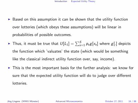
I Based on this assumption it can be shown that the utility function

over lotteries (which obeys these assumptions) will be linear in

probabilities of possible outcomes.

I Thus, it must be true that U[L1] =∑S

s=1 psg [xs ] where g [.] depicts

the function which ’valuates’ the state (which would be something

like the classical indirect utility function over, say, income).

I This is the most important basis for the further analysis: we know for

sure that the expected utility function will do to judge over different

lotteries.



I Proving this ’linearity’ of the utility function is done in several steps.

I First of all we will argue that any lottery i can be characterized by a

specific number αi .

I Consequently, we can find a function that maps the set of lotteries

into this set of numbers which represents the preference relation.



I Consider in the set of lotteries L the best L and the worst L lottery.

I We want to show that any lottery can be represented by a specific

number. Suppose this was not the case (Contradiction)

I If this was not the case, it would be true that for some lottery L it

holds that L ∼ α1L + (1− α1)L︸︷︷︸L1

I and L ∼ α2L + (1− α2)L︸︷︷︸L2



I We are going to show is that for α1 6= α2 (given the stated axioms),

this cannot be true.

I Suppose (for expository reasons) that α1 > α2

I We can write L1 = α1L + (1− α1)[ L21−α2

− α21−α2

L]

I which simplifies to L1 = γL + (1− γ)L2 with γ := α1−α21−α2



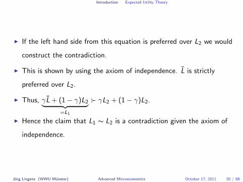
I If the left hand side from this equation is preferred over L2 we would

construct the contradiction.

I This is shown by using the axiom of independence. L is strictly

preferred over L2.

I Thus, γL + (1− γ)L2︸︷︷︸=L1

� γL2 + (1− γ)L2.

I Hence the claim that L1 ∼ L2 is a contradiction given the axiom of

independence.



I Thus, we can claim that any lottery i can be characterized by a

specific number αi for which holds that L1 � L2 implies that α1 > α2.

I This basically implies that the utility of any lottery can be ranked

according to this number.

I Thus, the utility function must ensure that U[Li ] = αi to represent

the preference relation (where αi makes the agent indifferent between

Li and the mixture of the best and the worst lottery.).

I Using this insight, we can show that the claimed utility function is

linear.



I Linearity implies that for any two lotteries, say, L1 and L2 it must be

true that U[αL1 + (1− α)L2] = αU[L1] + (1− α)U[L2] where

α ∈ [0, 1] is some arbitrary number.

I For the utility function it must be true that U[Li ] = αi and by

definition we know that Li ∼ αi L + (1− αi )L

I So by means of definitions we can write for any lottery Li :

Li ∼ U[Li ]L + (1− U[Li ])L



I So we can write

αL1 + (1− α)L2 ∼

α(U[L1]L + (1− U[L1])L) + (1− α)(U[L2]L + (1− U[L2])L)

I Which can be written as

L3 = αL1 + (1− α)L2 ∼ α3L + (1− α3)L

with α3 := αU(L1) + (1− α)U(L2)

I Using all this, we know that α3 is the specific number which

characterizes the mixed lottery (L1, L2, α).



I Thus, it must be true that U[αL1 + (1− α)L2] = α3 by definition.

I Moreover, by our definition αU[L1] + (1− α)U[L2] = α3.

I Consequently, U[.] must be linear.



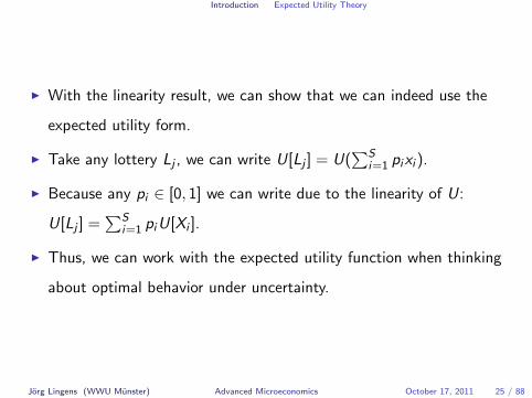
I With the linearity result, we can show that we can indeed use the

expected utility form.

I Take any lottery Lj , we can write U[Lj ] = U(∑S

i=1 pixi ).

I Because any pi ∈ [0, 1] we can write due to the linearity of U:

U[Lj ] =∑S

i=1 piU[Xi ].

I Thus, we can work with the expected utility function when thinking

about optimal behavior under uncertainty.



I This is a very powerful result since it provides the analytic basis a

wide array of applications in Microeconomics.

I Note that although the expected utility theory is often assumed to be

straightforward or just taken for granted this is not the case.

I Why shouldn’t it be the true that e.g. the variance or some other

moment would affect the preference relation of the agent?

I The rigorous proof shows that only the probability weighted ’state

utility’ matters for behavior (as long as we accept the independence

axiom).


Date post:	15-May-2018
Category:	Documents
Upload:	dophuc
View:	228 times
Download:	1 times

Advanced Microeconomics - The Economics of Uncertainty · Advanced Microeconomics - The Economics...

Documents