Advanced Optical Communications Prof. R.K. Shevgaonkar

Department of Electrical Engineering Indian Institute of Technology, Bombay

Lecture No. # 10

Signal Distortion – III

We are discussing signal distortion on optical fibers. So, first we discussed what is called

dispersion, which is essentially the pulse broadening as the pulse travels on the optical

fiber. Then we went to another aspect that was attenuation, and then we saw there are

various mechanisms by which the pulse energy is lost, when it propagates on the fiber.

(Refer Slide Time: 00:59)

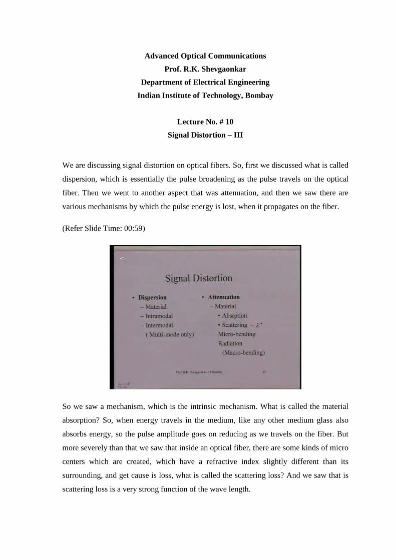
So we saw a mechanism, which is the intrinsic mechanism. What is called the material

absorption? So, when energy travels in the medium, like any other medium glass also

absorbs energy, so the pulse amplitude goes on reducing as we travels on the fiber. But

more severely than that we saw that inside an optical fiber, there are some kinds of micro

centers which are created, which have a refractive index slightly different than its

surrounding, and get cause is loss, what is called the scattering loss? And we saw that is

scattering loss is a very strong function of the wave length.

So, it goes as lambda to the power minus 4, that means every doubling of the wave

length the scattering loss reduces by factor of 16. Now, these two losses are present

inside the optical fiber even before the fiber was commission into the system; was the

fiber is commission into the system, there are two more additional losses taking place

and they are what are called the micro bending losses, and the radiation losses. So, it

some micro bending loss is the loss, where if the fiber is deformed over micro scales,

then locally is some leakage of energy take place, and that loss is called the micro

bending loss.

Now, another loss which is of importance is what is called the radiation loss and that is if

the fiber is gently bend to over a large arc and if the radius of that arc is much larger

compare to the wave length, then you have a leakage of energy and that is what is called

the radiation loss. So, that is understood when the fiber is gently bend why the radiation

takes place from the optical fiber. So, first let us consider the fiber which is the straight

fiber.

(Refer Slide Time: 03:10)

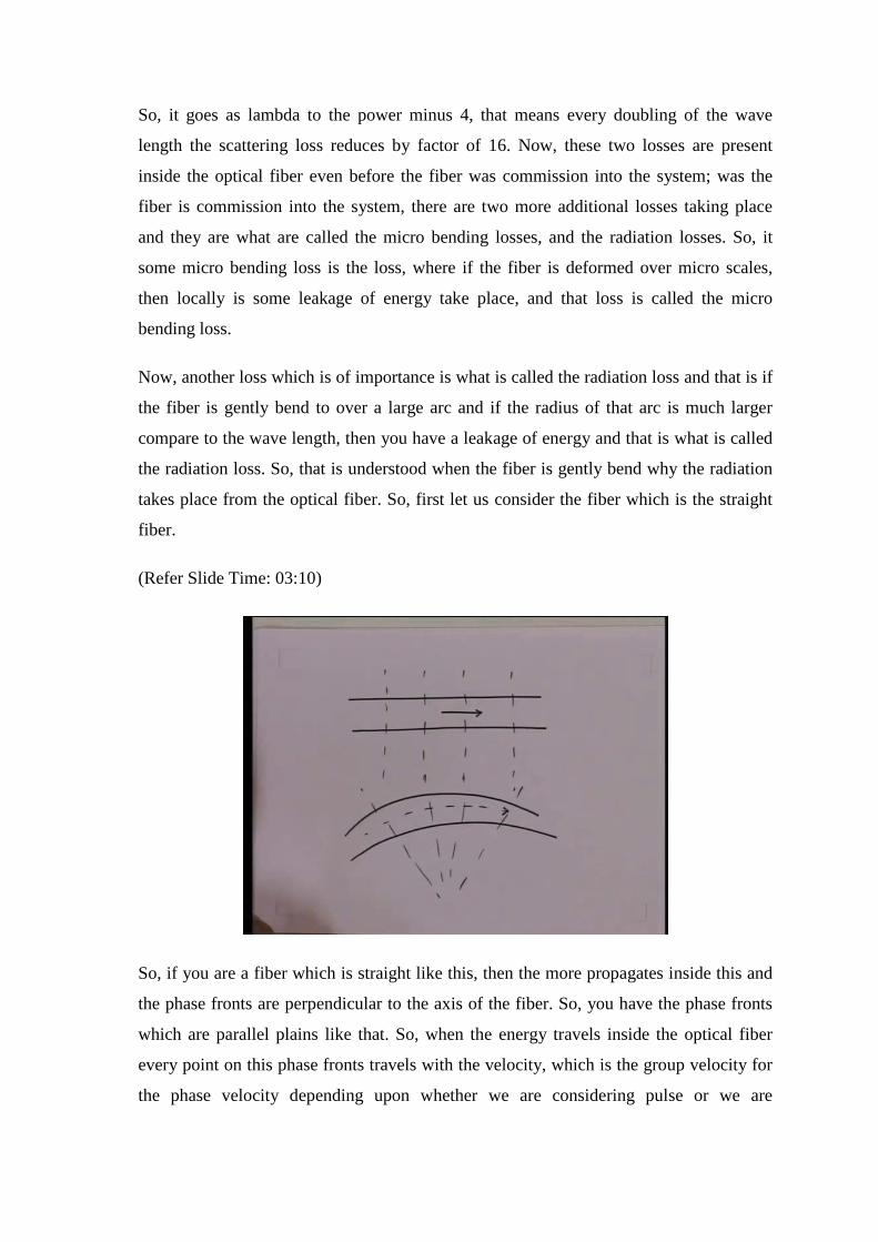
So, if you are a fiber which is straight like this, then the more propagates inside this and

the phase fronts are perpendicular to the axis of the fiber. So, you have the phase fronts

which are parallel plains like that. So, when the energy travels inside the optical fiber

every point on this phase fronts travels with the velocity, which is the group velocity for

the phase velocity depending upon whether we are considering pulse or we are

considering continues signal, but important thing do not here is that every point on this

phase front moves with the same speed. However, now if I gently bend the fiber then the

fiber becomes and arc like that.

So, this the fiber now and now the phase fronts arc again perpendicular to the direction

of propagation, but direction is now become along this arc. So, the face fronts are no

more parallel, but they are like the fans which are devoted to the center of curvature of

this arc. So, you have a phase fronts which will look something like this, something like

this, something like this, something like this and so on. So, in the first case when the

fiber was absolutely state the phase fronts where parallel to each other whereas, when the

fiber is bend then the phase fronts move like a fan which are pivoted to the center of

curvature of this arc.

Now when that happens, every point on the phase fronts now does not move with the

same speed. Because the point which are closer toward the center of curvature, they

move with the lower velocity as you go further and further the velocity increases and

very soon, you will list to a region for gives to a distance, where the velocity becomes

equal to velocity of light intrinsically in that medium and beyond that then the velocity

cannot increase.

So, as a result the energy which is beyond that distance that cannot propagate along with

this mode now so, that energy slowly detaches itself and stars leaking from this structure

this is the one which is what is called the radiation loss. So, important thing to note here

is that no matter how gentle the bend e your always find it distance at which the velocity

will try to become greater than the velocity of light intrinsically in that medium and the

either g will leak out.

(Refer Slide Time: 06:18)

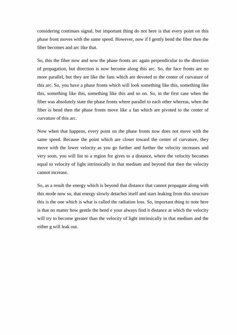
So, now the two things to observe here, that one I consider a bending loss and let us say

if I consider a model distribution which is something like this. This is the distance at

which the velocity becomes equal to velocity of light in that medium what that means, is

this that this now energy, which is in this region store by the hatch region, that energy

cannot propagate along with this mode. Because, it requires velocity greater than the

velocity of light that medium and then this energy will essentially detach and will

contribute to the radiation loss. Now, since the energy which is leaving from here in the

mode has to be maintain like this as soon as this energy is lost for continuity of the fields

again the fields have to be generated.

So, power is drawn from power which is flowing inside the fiber. So, there is a net loss

power which is going to take place in energy which is flowing inside the core of the

fiber. Now, seen this is the energy which is going be radiated the amount of energy,

which will get radiated will depend upon how close this distance is from the core.

Secondly, how spreaded this field is inside the cladding. The first thing is very clear that

as you bend the fiber more and more, the radios of curvature will decrease and because

of this distance will come closer and closer. So, sharper you bend the optical fiber more

will be the radiation loss, because closer will be this distance and this energy will go on

increasing.

Similarly, if I consider a mode whose field is much spreaded inside the cladding then for

a given bend more energy will be radiated, because you will have more electric field

amplitude beyond the distance at which the velocity become greater than velocity of light

in that medium and we know from our model analysis that as we go to higher and higher

order modes the more and more field now is inside the cladding. So, what that means, is

for a given bend higher order of modes will suffer more radiation loss, because there

field is going to be more spreaded inside the cladding and lower order modes will be list

of effected.

So, as a important thing it we get from here is that whenever we consider fiber and if the

fiber is bend then the energy is going to is leak out from this and sharper the bend more

will be the energy loss form that bend and higher the mode more will be the energy loss

for a given bend. However, one can calculate this analysis is not very trivial you got (( ))

very regress analysis to calculate what is called the radiation loss and what can be shown

is that the radiation loss is a very strong function of this radius. So, if you bend the fiber

very gently and if the radius of curvature is of the order of tends of centimeter the

radiation loss is practically negligible.

But, if you consider the radius of curvature of the order of about few centimeters, then

this radiation loss increases very rapidly. So, if one most avoid the radiation loss while

laying the fiber one should make sure that the fiber loops of the size of few centimeter

should not be formed, otherwise one would have a very heavy radiation loss. This also

gives something interesting that if you consider a fiber which is trade and whether is no

energy leaking from here, because the mode is completely guided. One would never be

able to tell whether the fiber is illuminated or not illuminated, because there is no

leakage of energy and unless the energy reaches to an observe from outside.

One would not be able to tell whether the fiber is carrying light or it is not carrying light.

So, if the fiber is kept in absolutely straight position then looking at the fiber one would

not be able to tell whether the fiber is lit or not lit. But you take the fiber and you bend

it then because of the radiation loss the energy will start leaking and then one can see the

light emitted from the bend. So, by bending just a fiber one can see the light coming out

and this light can be seeing in from outside, if it is in the visible range or can be

measured form by instrument if it is in the invisible rate. But the important thing to not at

this point be that if the fiber is bending then energy can leak very easily from the fiber.

Now, recall when we are talking about the characteristics of optical communication in

very first lecture, we are said that optical communication is very secure; that means, no

data can be tapped when the information flows inside the optical fiber what we however,

seen how is that if you take a fiber and just bend it the energy can simply leak from the

fiber and the signal can be tapped. But in practical fiber you always have the covering

shields which will not allow you to tab the light which is radiated by the bend fiber. So,

if we had bear fiber then of course, yesterday the fiber is bend the light will get emitted

and there will be leakage of power.

But, if you consider a fiber which is having jackets an all that then even the radiated light

will not be detected and you seal have a security in your communication. So, this is the

important aspect whenever, we lay a fiber inside is system that fiber should not form will

you small loops, because you do that than you would have the axis loss over and above

the intrinsic loss in the optical fiber. So, putting all effects together then one gets the

losses in a system, which are much higher compare to what intrinsically and optical fiber

is capable of giving.

Also you would not that when we go for a wave length 1550 nanometer. Since, that

wavelength v number is smaller comparing to 1310 nanometer the energies model

energies spread much more in the cladding. So, all this losses have a higher contribution

at 1550 compare to 1310. So, those theoretically we see that the attenuation for glass is

minimum at 1550 nanometer and 1310 nanometer losses are higher. In practice, when the

fiber is led in the system in variably, we find that the losses at 1550 are comparable or

higher than 1310, because this losses the micro bending losses and the radiation losses

they become large at 1550 nanometer compare to 1310 nanometer.

Let us now come back again to our discussion on the dispersion. That means, saw that

when we consider a dispersion in the single mode optical fiber we saw that the dispersion

comes because of two components, one is because of the intrinsic material dispersion

and other one we saw is the dispersion, which is because of the wave guiding nature and

we also saw that the material dispersion is not in our control, because first the material

glass has been identified practically the material dispersion is fixed. However, the wave

light dispersion which depends upon the fiber parameters, the size of the fiber, and the

refractive index profile of the fiber these quantities are can be manipulated by changing

the fiber parameters.

So, what we know find interesting is that the total dispersion which we see on the optical

fiber, which is always a combination of the material dispersion and the wave guide

dispersion that can be manipulated by controlling the fiber parameters and thus every

interesting option, because if we recall when we talked about dispersion and loss we find

that 1310 nanometer wave length is the wave length were dispersion is minimum, but the

loss is about 0.2 to 0.3 db higher. If you go to 1550 nanometer then the loss is minimal

there, but the dispersion is about minus 20 picoseconds per kilometer nanometer.

So, either you could operate a wave length where loss is minimum which is 1550, but

then you have a larger pulse broadening or lesser bandwidth or you can operate at 1310

nanometer, where the bandwidth is large, but the loss higher. As we said earlier for a

good communication, we would like to get both we should have a low loss and we

should have a large bandwidth. So, in earlier situation either you could get bandwidth or

you could get the loss because this two wave length 1310 and 1550, there offering one at

a time.

However, once you find now the fact that the dispersion can be manipulated why

controlling the fiber parameters, then immediately one can proceed to find out whether

one can shift the zero dispersion point which was a 1310 nanometer to 1550 nanometer.

So, if you could manipulate the wave guide dispersion then there is possibility, that the

zero dispersion point can be shifted to some other wave length and if that option is

available immediately one would like shifted wave length which is 1550 nanometer,

because that is the wave length were the losses minimum.

So, if you could teller the fiber such that the zero dispersion fiber for this wave length for

this fiber is at 1550 nanometer, then one can have both we have loss and we will have a

very large bandwidth, because dispersion will be zero. Precisely, thus what essentially is

done in is what is called the dispersion shifted fibers.

(Refer Slide Time: 18:15)

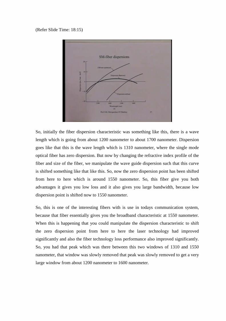
So, initially the fiber dispersion characteristic was something like this, there is a wave

length which is going from about 1200 nanometer to about 1700 nanometer. Dispersion

goes like that this is the wave length which is 1310 nanometer, where the single mode

optical fiber has zero dispersion. But now by changing the refractive index profile of the

fiber and size of the fiber, we manipulate the wave guide dispersion such that this curve

is shifted something like that like this. So, now the zero dispersion point has been shifted

from here to here which is around 1550 nanometer. So, this fiber give you both

advantages it gives you low loss and it also gives you large bandwidth, because low

dispersion point is shifted now to 1550 nanometer.

So, this is one of the interesting fibers with is use in todays communication system,

because that fiber essentially gives you the broadband characteristic at 1550 nanometer.

When this is happening that you could manipulate the dispersion characteristic to shift

the zero dispersion point from here to here the laser technology had improved

significantly and also the fiber technology loss performance also improved significantly.

So, you had that peak which was there between this two windows of 1310 and 1550

nanometer, that window was slowly removed that peak was slowly removed to get a very

large window from about 1200 nanometer to 1600 nanometer.

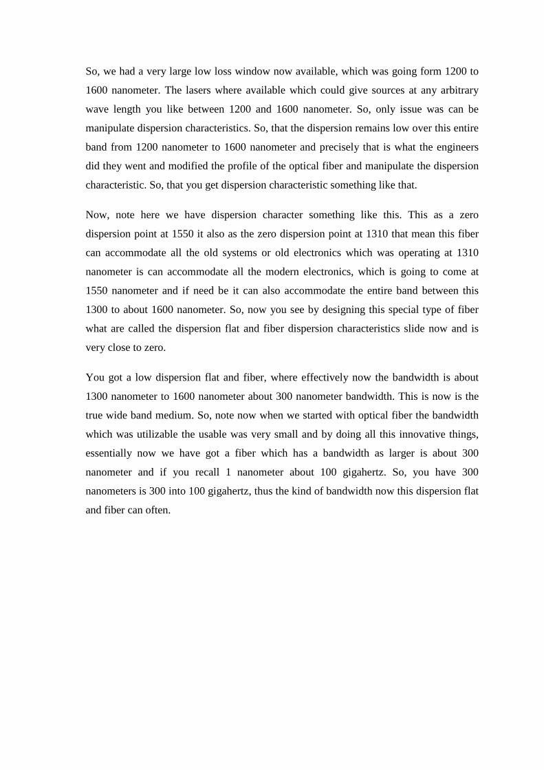
So, we had a very large low loss window now available, which was going form 1200 to

1600 nanometer. The lasers where available which could give sources at any arbitrary

wave length you like between 1200 and 1600 nanometer. So, only issue was can be

manipulate dispersion characteristics. So, that the dispersion remains low over this entire

band from 1200 nanometer to 1600 nanometer and precisely that is what the engineers

did they went and modified the profile of the optical fiber and manipulate the dispersion

characteristic. So, that you get dispersion characteristic something like that.

Now, note here we have dispersion character something like this. This as a zero

dispersion point at 1550 it also as the zero dispersion point at 1310 that mean this fiber

can accommodate all the old systems or old electronics which was operating at 1310

nanometer is can accommodate all the modern electronics, which is going to come at

1550 nanometer and if need be it can also accommodate the entire band between this

1300 to about 1600 nanometer. So, now you see by designing this special type of fiber

what are called the dispersion flat and fiber dispersion characteristics slide now and is

very close to zero.

You got a low dispersion flat and fiber, where effectively now the bandwidth is about

1300 nanometer to 1600 nanometer about 300 nanometer bandwidth. This is now is the

true wide band medium. So, note now when we started with optical fiber the bandwidth

which was utilizable the usable was very small and by doing all this innovative things,

essentially now we have got a fiber which has a bandwidth as larger is about 300

nanometer and if you recall 1 nanometer about 100 gigahertz. So, you have 300

nanometers is 300 into 100 gigahertz, thus the kind of bandwidth now this dispersion flat

and fiber can often.

(Refer Slide Time: 22:43)

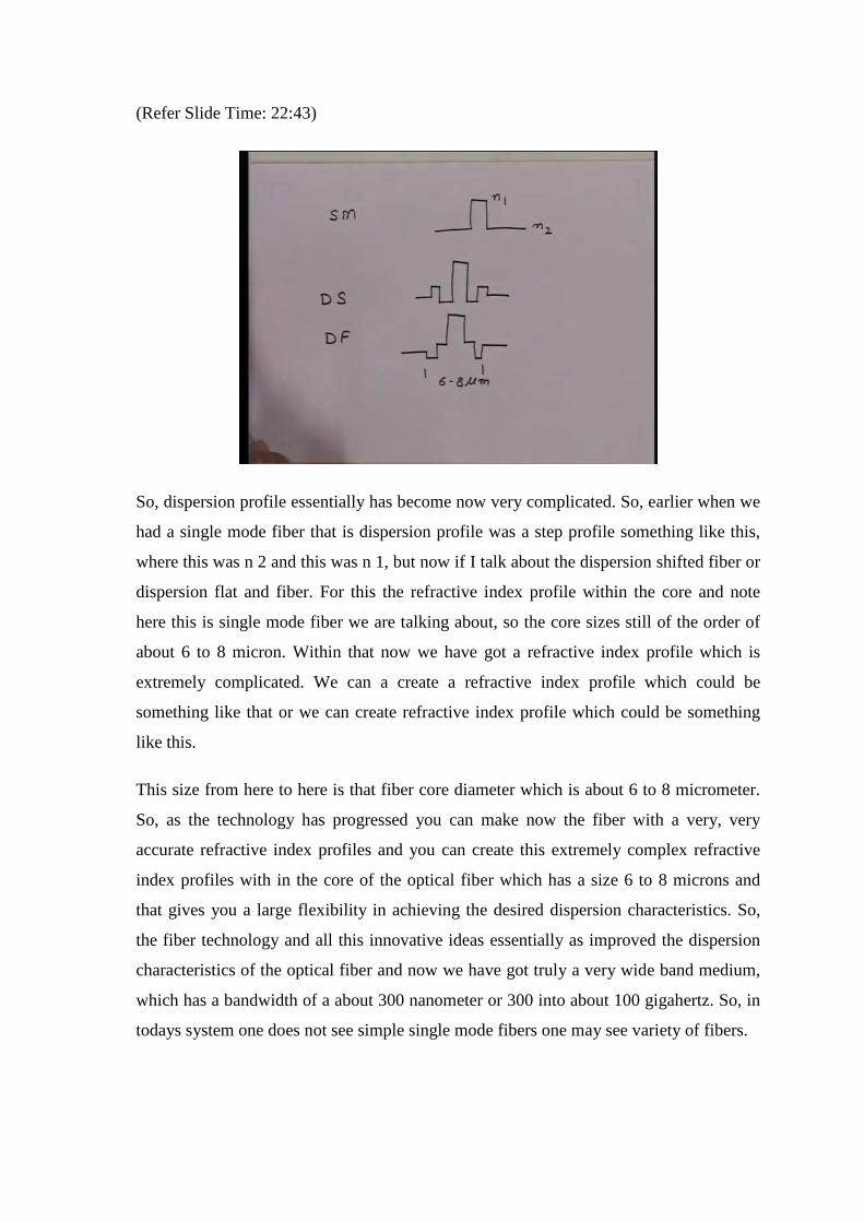
So, dispersion profile essentially has become now very complicated. So, earlier when we

had a single mode fiber that is dispersion profile was a step profile something like this,

where this was n 2 and this was n 1, but now if I talk about the dispersion shifted fiber or

dispersion flat and fiber. For this the refractive index profile within the core and note

here this is single mode fiber we are talking about, so the core sizes still of the order of

about 6 to 8 micron. Within that now we have got a refractive index profile which is

extremely complicated. We can a create a refractive index profile which could be

something like that or we can create refractive index profile which could be something

like this.

This size from here to here is that fiber core diameter which is about 6 to 8 micrometer.

So, as the technology has progressed you can make now the fiber with a very, very

accurate refractive index profiles and you can create this extremely complex refractive

index profiles with in the core of the optical fiber which has a size 6 to 8 microns and

that gives you a large flexibility in achieving the desired dispersion characteristics. So,

the fiber technology and all this innovative ideas essentially as improved the dispersion

characteristics of the optical fiber and now we have got truly a very wide band medium,

which has a bandwidth of a about 300 nanometer or 300 into about 100 gigahertz. So, in

todays system one does not see simple single mode fibers one may see variety of fibers.

So, now let be just summarize what we have seen up till now. We started with a simple

model on the optical fiber. We saw the fiber which was multimode optical fiber and we

saw that there is a multimode optical fiber is only of academic interest normally

dispersion of this fiber is very large. Then we said without sacrificing the launching

efficiency or without reducing the core size to much one could reduce the dispersion by

making the fiber what is called greater index optical fiber and these are the fibers which

normally are use in practice.

So, in local area networks where data rate is not very large, the fiber which are used are

the greater index of the optical fibers and then we saw that if you go to very long

distance communication, then the fiber which one has use is what is called single mode

optical fiber and single mode optical fiber has a zero dispersion intrinsically at 1310

nanometer. Then to achieve a low dispersion at 1550 nanometer wave length we

modified the refractive index profile and then we got another class of fiber what is called

a dispersion shifted fiber.

And then to accommodate large number of wavelengths between 1300 nanometer and

1550 nanometer, we design another class of fiber what is called the dispersion flat and

fibers. So, in todays system essentially this all types of fibers are use depending upon

what are the distances and what kind of bandwidth we are using and how many channel

transmission we have a into optical communication. one can however, now ask a basic

question the earlier when I had a fiber something like this where I had core refractive

index n 1 and cladding refractive index n 2. We define this quantity what is called the v

number which was 2 pi upon 1 lambda into core radius into numerical aperture which

was square root of n 1 square minus n 2 square.

But, if you have a refractive index profile which is complex likes this. What is n 1 and

what is n 2? In fact there is no the single core here, one can say you are having multiple

shells. The whole thing is now we are calling is core from here to here. So, you have

inner region and then you have a ring around return that ring around return, you have a

multiple cladded region that we call a score and then where the refractive index become

constant that essentially we call as cladding. So, first into note here is there is a no n 1

the n 2 you may say is the refractive index of the cladding which is constant, but we want

know what is this quantity n 1 now.

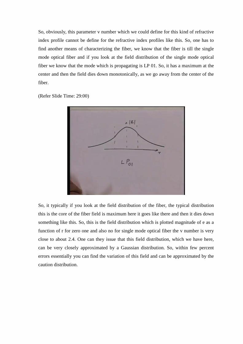
So, obviously, this parameter v number which we could define for this kind of refractive

index profile cannot be define for the refractive index profiles like this. So, one has to

find another means of characterizing the fiber, we know that the fiber is till the single

mode optical fiber and if you look at the field distribution of the single mode optical

fiber we know that the mode which is propagating is LP 01. So, it has a maximum at the

center and then the field dies down monotonically, as we go away from the center of the

fiber.

(Refer Slide Time: 29:00)

So, it typically if you look at the field distribution of the fiber, the typical distribution

this is the core of the fiber field is maximum here it goes like there and then it dies down

something like this. So, this is the field distribution which is plotted magnitude of e as a

function of r for zero one and also no for single mode optical fiber the v number is very

close to about 2.4. One can they issue that this field distribution, which we have here,

can be very closely approximated by a Gaussian distribution. So, within few percent

errors essentially you can find the variation of this field and can be approximated by the

caution distribution.

(Refer Slide Time: 30:11)

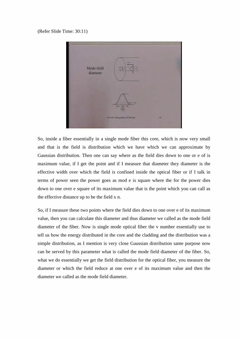
So, inside a fiber essentially in a single mode fiber this core, which is now very small

and that is the field is distribution which we have which we can approximate by

Gaussian distribution. Then one can say where as the field dies down to one or e of is

maximum value, if I get the point and if I measure that diameter they diameter is the

effective width over which the field is confined inside the optical fiber or if I talk in

terms of power seen the power goes as mod e is square where the for the power dies

down to one over e square of its maximum value that is the point which you can call as

the effective distance up to be the field x n.

So, if I measure these two points where the field dies down to one over e of its maximum

value, then you can calculate this diameter and thus diameter we called as the mode field

diameter of the fiber. Now is single mode optical fiber the v number essentially use to

tell us how the energy distributed in the core and the cladding and the distribution was a

simple distribution, as I mention is very close Gaussian distribution same purpose now

can be served by this parameter what is called the mode field diameter of the fiber. So,

what we do essentially we get the field distribution for the optical fiber, you measure the

diameter or which the field reduce at one over e of its maximum value and then the

diameter we called as the mode field diameter.

So, for a single mode optical fiber this has a complex refractive index profile. The mode

field diameter is much more meaning full quantity then defining the v number, because

number cannot be define for this complex refractive index structures. Now, mode field

diameter is a important parameter, because suppose we have different fibers and we want

to combine this because and in a system you may not have only one type of fiber, which

can be running many time you may get fibers coming from different companies, different

manufacturers and you have to make a joint between this fibers.

Obviously, if the light which is coming out of one fiber does not match with the other

fiber in terms of its numerical aperture cone, then you will not have a guiding of the light

efficiently from one fiber to another fiber. So, if I have the fiber which are of different

nature which have different refractive index profile which have different sizes there, how

do I say whether this two fibers are comparable. So, one can show that if you make the

mode field diameters of the two fibers same, then there is a perfect launching from one

fiber to another and there is no loss at the junction where the two fibers are connect.

So, essentially whenever we want to make a joint between two fibers without varying

about what are their actual parameters are like, what is the diameter of the core, what is

the refractive in the profile of the core, you simply ask only one parameter and that is the

mode field diameter of the fiber. If the two fibers have mode field diameter same, then

they can be joint without a loss of light launching efficiency and thus wise parameter is a

very important parameter.

(Refer Slide Time: 34:39)

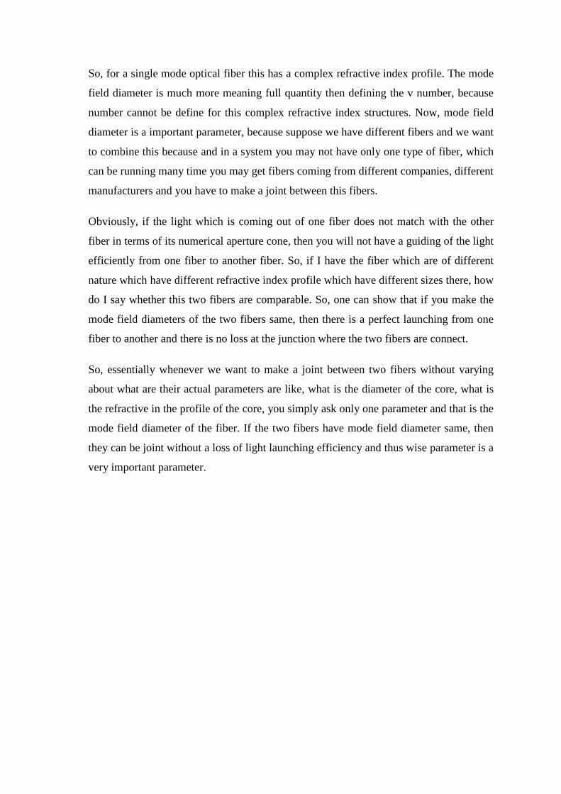
The loss which takes place because of the mode filed diameter that is essentially given

by the loss that is equal to 2 upon MFD 1 upon MFD 2 plus MFD 2 upon MFD 1. We

can put in terms of the logarithm in terms of db so, I can take log 10. So, note here MFD

1 and MFD 2 are equal this is one, this is one so this ratio will be one log of that will be

0. So, we will have a 0 db loss whereas, when these two diameters are not equal then

from here approximately, you can calculate how much will be the loss at the junction

when the two different types of fibers are joint.

So, MFD is therefore, one of the important parameters whenever we want to characterize

now a single mode optical fiber, which has a complex refractive index profiles. Like this,

there are many other parameters also which are required two characterize the fiber

completely, when the fiber is late into the system and another parameter which is of

importance is what is call the birefringence of an optical fiber.

(Refer Slide Time: 36:30)

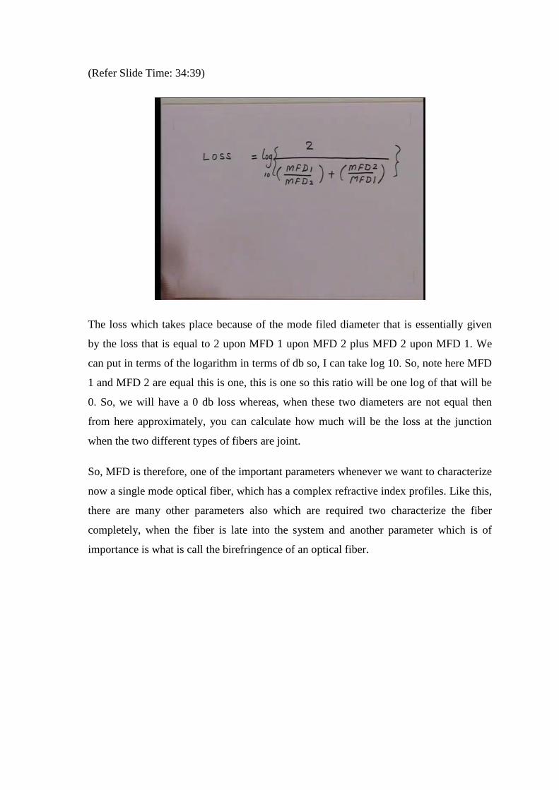
So, we have another parameter what is called birefringence of a fiber and this quantity is

defined as follows. We have seen that if you consider the optical fiber with a core which

is absolutely circular, then we can launch a light which is linearly polarize which can be

decompose into two orthogonal polarizations. So, let us say I have two linearly polarize

mode one has polarization like this and other one has polarization which will be

horizontal. So, if the fiber is absolutely circular any arbitrary direction of the electric

field can be decompose into two.

So, we say that we have two degenerate LP 01 modes with perpendicular polarization

and since the fiber is absolutely circular both the polarization sees the same phase

constant or they travel with the same speed. If there happens then the state of

polarization is maintained, because both of this fields are going to undergo the same

phase change go a distance and when the combine again the generate the same state of

polarization. However in practice the fiber is not absolutely circular because of the

manufacturing process and so on, the fiber has small ellipticity.

So that means, the effective radius which the vertical polarization since not same as the

radius with the horizontal polarization or in other word what we saying is the v number,

which this polarization since different than the v number which this polarizations. Since,

the v number changes from the b v diagram, we know that the phase constant also will

change.

So that means, we have the phase constant for two polarization for the same LP 01 mode

could be different and if I define the phase constant why beta naught as we seen earlier

we get a quantity what is called the effective index of model propagation. So, what this is

telling you that in the real fiber the effective index for horizontal polarization and

vertical polarization could be different. So, let us say that effective index is defined by n

x and we defined by n y. So, due to a small ellipticity in the core of the optical fiber the

model index c in by horizontal and vertical polarizations is not same. So, a difference in

these two different refractive indices is what is called the birefringence of the optical

fiber. So, we define this quantity birefringence that is equal to n y minus n x.

Now, what does the birefringence do? Firstly, it will be immediately clear that the phase

constant of this polarization we will be beta naught into n y and the phase constant of this

polarization will be beta naught into n x and since omega by beta is the phase velocity,

the phase velocity for this and this could be different. So, initially let us say we had a

linear polarization launched inside the optical fiber, which could be decompose into this

two components that you may recall in linear polarization both the components are in

phase.

So, to start with we have a polarization which will generate this two component which

are in phase and thus signal travels on the fiber this thing will go undergo a phase

change, which is beta naught into n y and this thing will undergo a phase change which

will beta naught into n x and since n y and n x naught equal essentially, there is the phase

difference between this two components and one there is a phase difference between the

two components the state of polarization is changed. So, if the phase difference between

this two becomes 90 degrees. The polarization will becomes circular any other phase

difference you will get a polarization with elliptical polarization.

(Refer Slide Time: 41:51)

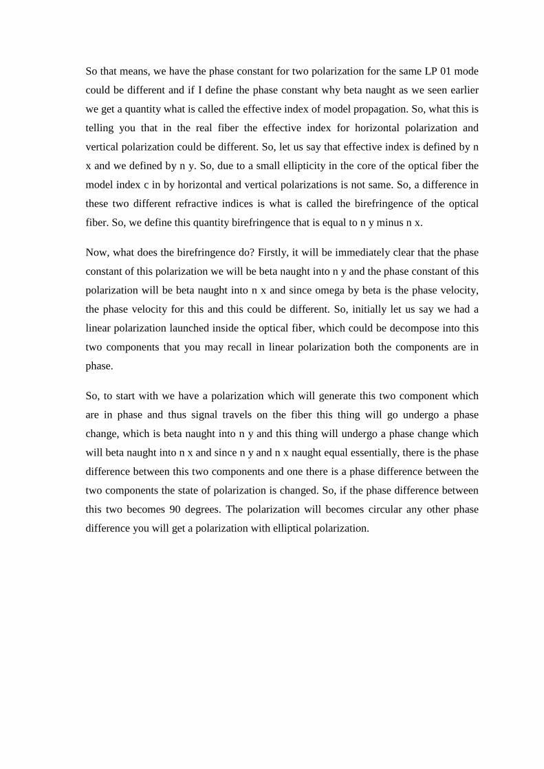
So, now what we see is that when the light propagates in an optical fiber in the single

mode, then let us says this is the fiber, light is propagating in this. Here the polarization

was linear when it was launched, let us say it was something like this, as you propagated

along the length slowly it become elliptical, then after certain distance it becomes

circular, because the phase difference at become 90 degrees, again the phase difference

will increase. So, again it will become elliptical, and so on, and linear and so on and so

forth. So, as the light travels along the optical fiber the state of polarization will go on

continuously changing distance over which this thing change us that we call as the beat

length on the optical fiber.

So, we can define what is called the beat length that is equal to 2 pi divided by difference

in the phase constants which is nothing, but beta naught into n y minus n x. So, this is the

distance now the beat length over which the phase difference would change by 2 pi so,

again the same polarization will be generated or from the distance. So, because of this

variation in the size of the core of the optical fiber the whole lot of things happen and

one of the thing which happens here is the what is called the change is state of

polarization. If I see in terms of the group velocity, the same thing will happen to group

velocity also that whatever pulse I launched inside this the pulse energy will get divided

into two polarizations horizontal and vertical and the two will travel with different group

velocities.

(Refer Slide Time: 44:22)

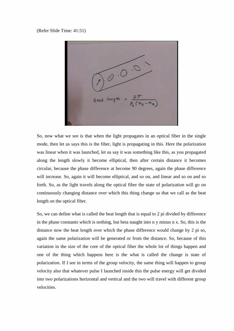
So, you will see that there is tendency for pulse to separate out because of this. So, if I

take now a fiber like this and if I launch a optical pulse the pulse energy will get divided

into two polarization one is this, one is this and as a travels because of the birefringence

variation inside the optical fiber. You will see that the two pulses will not reach at a same

time on the other side of the fiber. So, there will be a difference in this and again this

phenomenon is the statistical phenomena. So, you will not get a systematically this pulse

is moving forward of this is going ahead, there will be some kind of a jitter something

kind of thing will be developed because of this and you will have a effective broadening

of the pulse, because of this phenomena.

This is what is called the polarization mode dispersion and in fact this is the dispersion,

which is becoming bottle neck in the high speed communication. So, even if you go

design the fibers which are having very low dispersion is so on ultimate the limiting

factor would be what is called the polarization mode dispersion. So, this quantity also is

an important parameter in normal system where data rates are very small these factors do

not contribute, but when we talk about data rates of if you gigahertz or 10 gigahertz or

try to increase the data rate beyond, that then essentially all this factors distorts paying

role.

So, we see now the dispersion not only we have a material dispersion, intermodal

dispersion, but we also have what is call the polarization mode dispersion inside the

fiber. Another parameter which normally one defines for a practical fiber, which is what,

is called the cut of wave length of the optical fiber. Now, we know that when we talk

about a single mode optical fiber, the v number should be such that only one mode

propagates and ideally it should be as away from the cut of frequency of the next mode

which is the LP 11 mode. Because, if this v number is very close to the 2.4 then even

with the small manufacturing tolerances the LP 11 mode will get exited. So, energy will

get diverted to LP 11 mode and because of that you will have some kind of dispersion of

pulse broadening.

So, we want that you are v number should be as away from the cut of v number for the

next mode, thus require. So, as be define a cut of wave length is the wave length where

the next mode will get start exciting which is the LP 11. How do you quantitatively

measure? So, there are certain standards which are define for measuring the cut of wave

length and the standards are is follows you consider a about two meter long fiber and

excite this fiber with a tunable laser source which can excite both the LP 01 mode and

LP 11 mode in equal proportion . So, now, I have a fiber which is about two meter length

and then you exciting this fiber which has tunable laser source which can excite both the

modes LP 01 and LP 11.

(Refer Slide Time: 48:21)

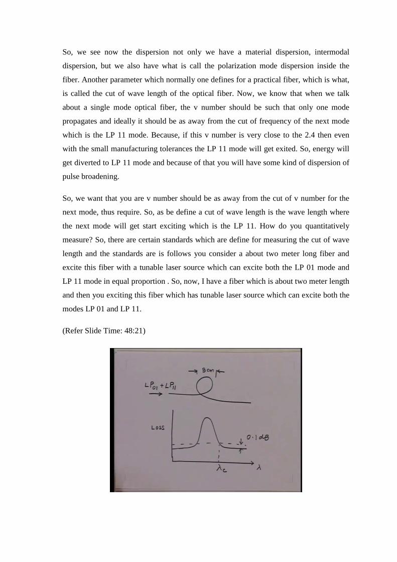
Now, let there be a loop formed because of this fiber. So, this fiber loop is of the order of

about let us say 3 centimeter, the light is launched inside this which launches LP 01 plus

LP 11. Now what we do is we measure the output power here as a function of the wave

length and measure the loss, essentially it decreases in power change in power as the

function of wave length. So, let us say suppose I measure the loss as a function of wave

length lambda. If I go to very small wave lengths, then both the modes are well excited

inside the optical fiber, there well confined inside the core and even with the bend in this

loop which essentially would normally give a radiation loss, since this both modes are

well inside the core the radiation loss on the negligibly small.

So, you will see most of the power appears at the output. So, the loss is very small, as we

increase the wave length and as you list two a wave length were now the LP 11 mode is

approaching cut off. If this more approaches cut of then it is energy spreads more in the

cladding and because of this loop now that energy is lost in very quickly. Because, we

saw that as you bend if you are having more energy inside the cladding there will be

more energy loss for that. So, as we increase the wave length, where the lambda becomes

close to the cut of wave length of LP 11.

You will see there will loss of in energy corresponding LP 11 and then will loss here will

increase. if I go to the wave length still further then LP 11 will not get excited at all,

because it will be will cut of and then the whole energy will we launched into LP 01

mode, which will not have loss inside this loop again and we will get almost the full

power coming here. So, if I look at now the typical loss profile it will look something

like this. So, initially you had the low loss because both modes where well guided inside

the core, then as you goes issue the cut of frequency the loss increases because energy

corresponding to LP 11 mode is radiate away and when I go on the other side, it will

longer wave length LP 11 does not get excited at all and seen the energy is confined to

only know LP 01 most of the energy again appears here.

So, standard says if you get this profile this longer wave length was the loss now is point

0.1 db with respect to this. So, thing is 0.1 db that wave length is what is called the cut of

wave length of the optical fiber and typically if you take a 1310 nanometer fiber, the cut

of wave length will be about 20 to 30 nanometer away from the wave length of

operation.

So, this is one of the important parameters whenever once specifies the fiber, the fiber

now is specify by various parameters it can be specified by is more fill diameter, it can

be specified by it dispersion characteristic, it can be specified by cut of wavelength. So,

whenever be specified fiber from the manufacturer this are the some of the parameters

which one as specified so that you can get the required fiber. So, you have what I have

we are done is we have essentially see in the general characteristics of optical fiber and

then we are now got certain parameters on the basis of which fiber can be specified like

the mode field diameter or the cut of wavelength or the dispersion or the loss and so on.

So, this more or less covers the discussion on the optical fiber, the basic propagation

characteristics of the optical fiber. So, next time when we meet we talk about other issues

related to optical fibers like manufacturing of optical fibers and so on, and then will go to

the other topics in this course, like optical sources and other things.