Advanced PID Control Optimisation and System ...

Advanced PID Control Optimisation and

System Identification for Multivariable

Glass Furnace Processes by

Genetic Algorithms

Kumaran Rajarathinam

A thesis submitted in partial fulfillment of the requirements of

Liverpool John Moores University for the degree of

Doctor of Philosophy

February 2016

i

To My Parents, Wife and Two Little Angles

Sekaran, Sarojini, Annaletchumy,

Niranjanaa and Hamssini

Acknowledgements

First and foremost, I would like to extend my gratitude and great appreciation to my

first Supervisor, Dr. Barry Gomm for his continual support, guidance and invaluable

advice throughout the duration of this PhD project. I would also like to thank my

second Supervisor Prof. DingLi Yu for his support and encouragement throughout

this research investigation.

Many individuals have unknowingly helped me in my research throughout my

PhD and therefore I would like to thank all of my fellow researchers and academics

at the Control Research Group at the Liverpool John Moores University for their

insight and experience. Without the fantastic research environment created by these

individuals, the completion of this project would not have been possible.

I would also like to acknowledge the support and encouragement of my friends

for their valuable contributions. Most importantly, my special thanks and deepest

appreciation to my parents, wife, children and all my family members. It is a

hackneyed theme to thank loved ones for patience and understanding while a project

is being undertaken, but now I know why, and do give heartfelt thanks.

Trademarks

MATLAB® is a registered trademark of The MathWorks, Inc.

SIMULINK® is a registered trademark of The MathWorks, Inc.

ii

Abstract

This thesis focuses on the development and analysis of general methods for the

design of optimal discrete PID control strategies for multivariable glass furnace pro-

cesses, where standard genetic algorithms (SGAs) are applied to optimise specially

formulated objective functions. Furthermore, a strong emphasis is given on the real-

istic model parameters identification method, which is illustrated to be applicable

to a wide range of higher order model parameters identification problems.

A complete, realistic and continuous excess oxygen model with nonlinearity ef-

fect was developed and the model parameters were identified. The developed excess

oxygen model consisted of three sub-models to characterise the real plant response.

The developed excess oxygen model was evaluated and compared with real plant dy-

namic response data, which illustrated the high degree of accuracy of the developed

model.

A new technique named predetermined time constant approximation was pro-

posed to make an assumption on the initial value of a predetermined time constant,

whose motive is to facilitate the SGAs to explore and exploit an optimal value for

higher order of continuous model’s parameters identification. Also, the proposed

predetermined time constant approximation technique demonstrated that the pop-

ulation diversity is well sustained while exploring the feasible search region and

exploiting to an optimal value. In general, the proposed method improves the SGAs

convergence rate towards the global optimum and illustrated the effectiveness.

An automatic tuning of decentralised discrete PID controllers for multivariable

processes, based on SGAs, was proposed. The main improvement of the proposed

technique is the ability to enhance the control robustness and to optimise discrete

iii

iv

PID parameters by compensating the loop interaction of a multivariable process.

This is attained by adding the individually optimised objective function of glass

temperature and excess oxygen processes as one objective function, to include the

total effect of the loop interaction by applying step inputs on both set points, tem-

perature and excess oxygen, at two different time periods in one simulation.

The effectiveness of the proposed tuning technique was supported by a number of

simulation results using two other SGAs conventional tuning techniques with 1st and

2nd order control oriented models. It was illustrated that, in all cases, the resulting

discrete PID control parameters completely satisfied all performance specifications.

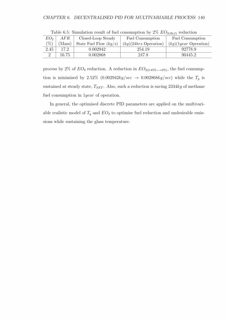
A new technique to minimise the fuel consumption for glass furnace processes

while sustaining the glass temperature is proposed. This proposed technique is

achieved by reducing the excess oxygen within the optimum thermal efficiency region

within 1.7% to 3.2%, which is approximately equal to about 10% to 20% of excess air.

Therefore, by reducing the excess oxygen set point within the optimum region, 2.45%

to 2%, the fuel consumption is minimised from 0.002942kg/sec to 0.002868kg/sec

while the thermal efficiency of the glass temperature is sustained at the desired set

point (1550K).

In addition, a reduction in excess oxygen within methane combustion guidelines

will assure that undesirable emissions are in control throughout the combustion

process. The efficiencies of the proposed technique were supported by a number

of simulation results applying the three SGAs controller tuning techniques. It was

illustrated that, in all cases, the fraction of excess oxygen reduction results in a great

minimisation of fuel consumption over long plant operating periods.

Contents

1 INTRODUCTION – OVERVIEW AND THESIS OUTLINE 1

1.1 Review of Glass Furnace Processes and Control . . . . . . . . . . . . 1

1.2 Problem Statement . . . . . . . . . . . . . . . . . . . . . . . . . . . 3

1.3 Research Novelty and Methodology . . . . . . . . . . . . . . . . . . . 3

1.4 Thesis Outline . . . . . . . . . . . . . . . . . . . . . . . . . . . . . . 5

1.5 Dissemination of Research Contributions . . . . . . . . . . . . . . . . 8

2 Literature Review of Optimisation and Genetic Algorithms 10

2.1 Introduction . . . . . . . . . . . . . . . . . . . . . . . . . . . . . . . . 10

2.2 Definition of Optimum . . . . . . . . . . . . . . . . . . . . . . . . . . 10

2.3 Overview of Optimisation Algorithms . . . . . . . . . . . . . . . . . . 11

2.3.1 Evolutionary Algorithm . . . . . . . . . . . . . . . . . . . . . 15

2.4 Standard Genetic Algorithms . . . . . . . . . . . . . . . . . . . . . . 17

2.4.1 Multi-Objective Optimisation by SGAs . . . . . . . . . . . . . 19

2.4.2 Premature Convergence . . . . . . . . . . . . . . . . . . . . . 19

2.4.3 SGAs in Model Parameter Identification . . . . . . . . . . . . 22

2.4.4 SGAs in Control Parameter Optimisation . . . . . . . . . . . . 24

2.4.5 An Application of SGAs for Furnace Type Processes . . . . . 26

2.5 Review of PID Control Strategies . . . . . . . . . . . . . . . . . . . . 27

2.6 Review of Multivariable PID Tuning Strategies . . . . . . . . . . . . 31

2.7 Why SGAs? . . . . . . . . . . . . . . . . . . . . . . . . . . . . . . . . 34

2.8 Chapter Summery . . . . . . . . . . . . . . . . . . . . . . . . . . . . 35

v

CONTENTS vi

3 Glass Furnace Modelling Validation 36

3.1 Introduction . . . . . . . . . . . . . . . . . . . . . . . . . . . . . . . . 36

3.2 Review of Combustion Chamber . . . . . . . . . . . . . . . . . . . . . 36

3.3 Combustion Chamber Modelling Approach . . . . . . . . . . . . . . . 38

3.3.1 Radiative Heat Transfer between Zones . . . . . . . . . . . . . 39

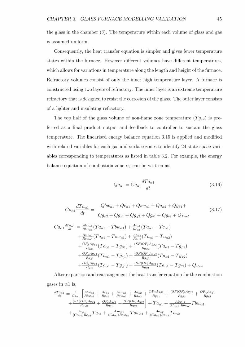
3.3.2 Energy Balance Equation . . . . . . . . . . . . . . . . . . . . 42

3.4 Simulated Combustion Chamber Model . . . . . . . . . . . . . . . . . 43

3.4.1 Brief Introduction of Glass Furnace . . . . . . . . . . . . . . . 46

3.4.2 Validation of Combustion Chamber Model . . . . . . . . . . . 47

3.5 Chapter Summary . . . . . . . . . . . . . . . . . . . . . . . . . . . . 51

4 Model Parameters Identification of Glass Temperature and Excess

Oxygen 53

4.1 Introduction . . . . . . . . . . . . . . . . . . . . . . . . . . . . . . . . 53

4.2 Model Parameter Identification . . . . . . . . . . . . . . . . . . . . . 54

4.2.1 Primary Elements of SGAs . . . . . . . . . . . . . . . . . . . . 55

4.2.1.1 Population Initialisation . . . . . . . . . . . . . . . . 55

4.2.1.2 Objective Function . . . . . . . . . . . . . . . . . . . 56

4.2.1.3 Selection . . . . . . . . . . . . . . . . . . . . . . . . 57

4.2.1.4 Crossover . . . . . . . . . . . . . . . . . . . . . . . . 58

4.2.1.5 Mutation . . . . . . . . . . . . . . . . . . . . . . . . 60

4.2.2 Prior Knowledge of Specific Problem . . . . . . . . . . . . . . 61

4.2.3 Convergence Constraints by Search Space Boundary . . . . . 62

4.2.4 Predetermined Time Constant Approximation . . . . . . . . . 63

4.2.5 Application of SGAs in Model Parameters Identification . . . 67

4.3 Glass Temperature (Tg) Model . . . . . . . . . . . . . . . . . . . . . . 71

4.3.1 Operating Point Selection of Tg . . . . . . . . . . . . . . . . . 72

4.3.2 Selection of Genetic Parameters . . . . . . . . . . . . . . . . . 73

4.3.3 Model Order Selection of Tg . . . . . . . . . . . . . . . . . . . 74

4.3.4 Simulation Results of Tg . . . . . . . . . . . . . . . . . . . . . 75

4.3.4.1 SBO Approximation for Tg by Open-Loop Technique 75

CONTENTS vii

4.3.4.2 Model Parameter Identification for Tg by SGAs . . . 75

4.4 Excess Oxygen (EO2) Model . . . . . . . . . . . . . . . . . . . . . . . 79

4.4.1 Methane Combustion Process . . . . . . . . . . . . . . . . . . 79

4.4.2 Complete EO2 Model Development . . . . . . . . . . . . . . . 83

4.4.3 Operating Point Selection of EO2 . . . . . . . . . . . . . . . . 85


4.4.5 Simulation Results of EO2 . . . . . . . . . . . . . . . . . . . . 85

4.4.5.1 SBO Approximation for EO2 by PTcA Method . . . 86

4.4.5.2 Model Order Selection of EO2 . . . . . . . . . . . . . 90

4.5 Summary . . . . . . . . . . . . . . . . . . . . . . . . . . . . . . . . . 96

5 CONTROL PARAMETERS OPTIMISATION OF GLASS TEM-

PERATURE AND EXCESS OXYGEN 98

5.1 Introduction . . . . . . . . . . . . . . . . . . . . . . . . . . . . . . . . 98

5.2 Brief Introduction of PID Control . . . . . . . . . . . . . . . . . . . 99

5.3 Discrete PID Parameters Optimisation . . . . . . . . . . . . . . . . . 100

5.4 SGAs Configuration for Control Optimisation . . . . . . . . . . . . . 101


5.5 Simulation Results of Control Oriented Models . . . . . . . . . . . . . 104

5.5.1 Performance Criteria Formulation . . . . . . . . . . . . . . . 105

5.5.2 Objective Function and Boundary Constraint Formulation on

EO2 . . . . . . . . . . . . . . . . . . . . . . . . . . . . . . . . 105

5.5.3 Objective Function and Boundary Constraint Formulation on

Tg . . . . . . . . . . . . . . . . . . . . . . . . . . . . . . . . . 109

5.6 Chapter Summary . . . . . . . . . . . . . . . . . . . . . . . . . . . . 118

6 Decentralised PID Controller Tuning for Multivariable Glass Fur-

nace Process 120

6.1 Introduction . . . . . . . . . . . . . . . . . . . . . . . . . . . . . . . . 120

6.2 Decentralised PID Control of Multivariable Glass Furnace Process . . 121

6.2.1 Control Oriented Optimisation Techniques . . . . . . . . . . . 123

CONTENTS viii

6.2.2 Simulation Results of Decentralised Control Oriented Model . 124

6.3 Decentralised PID Control of Realistic Multivariable Glass Furnace

Model . . . . . . . . . . . . . . . . . . . . . . . . . . . . . . . . . . . 129

6.3.1 Simulation Results of Realistic Multivariable Process Model . 130

6.3.1.1 Control Robustness and Loop Stability . . . . . . . . 131

6.3.1.2 Minimum Fuel Consumption . . . . . . . . . . . . . 134

6.4 Summary . . . . . . . . . . . . . . . . . . . . . . . . . . . . . . . . . 139

7 CONCLUSION – MAIN CONTRIBUTIONS AND FUTURE WORK

141

7.1 Introduction . . . . . . . . . . . . . . . . . . . . . . . . . . . . . . . . 141

7.2 Summary of Main Contributions . . . . . . . . . . . . . . . . . . . . . 141

7.2.1 Realistic EO2 Model Development . . . . . . . . . . . . . . . 142

7.2.2 PTCAMethod for Higher Order Model Parameters Identification142

7.2.3 Automatic Tuning Technique for Multivariable Processes . . . 143

7.2.4 Reduction of Fuel Consumption for Glass Furnace Process . . 144

7.3 Achieved Objectives . . . . . . . . . . . . . . . . . . . . . . . . . . . 145

7.4 Recommendations for Further Work . . . . . . . . . . . . . . . . . . . 146

7.4.1 Comparison of SGAs with other Tuning Approaches . . . . . . 146

7.4.2 Improvement on PTCA Method . . . . . . . . . . . . . . . . . 147

7.4.3 Automatic Search Space Boundary Resizing . . . . . . . . . . 148

7.4.4 Extension of Single Stage Multivariable Process to Multistage

Multivariable Process . . . . . . . . . . . . . . . . . . . . . . . 148

7.5 Summary . . . . . . . . . . . . . . . . . . . . . . . . . . . . . . . . . 150

References 151

Appendix 172

List of Figures

1.1 Schematic Flow of Research Methodology . . . . . . . . . . . . . . . . 4

2.1 Global and local maxima and minima . . . . . . . . . . . . . . . . . . 11

2.2 Schematic of generalised evolutionary algorithm (Fleming and Purs-

house, 2002) . . . . . . . . . . . . . . . . . . . . . . . . . . . . . . . . 16

2.3 Efficiency of different classes of search techniques across a problem

continuum (Goldberg, 1989) . . . . . . . . . . . . . . . . . . . . . . . 18

2.4 Phenomenon of initial population . . . . . . . . . . . . . . . . . . . . 20

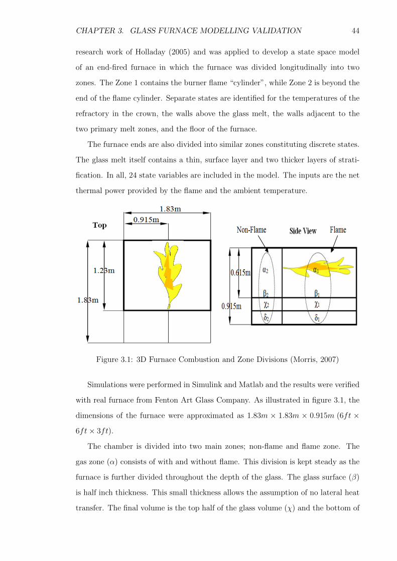
3.1 3D Furnace Combustion and Zone Divisions (Morris, 2007) . . . . . . 44

3.2 Block Diagram of Multivriable Glass Furnace . . . . . . . . . . . . . 47

3.3 Eigenvalues of 24 Original State-Space Variables (Unstable) . . . . . 48

3.4 Eigenvalues of Corrected 24 State-Space Variables (Stable) . . . . . . 48

3.5 Simulink Diagram of the Subsystem in the Open-Loop Model of Furnace 50

3.6 Step Responses of Glass Temperature of 3 Input Configurations . . . 51

4.1 Schematic diagram of model parameters to be optimised . . . . . . . 54

4.2 Gradual fitness improvements by SGAs execution (minimisation) . . . 57

4.3 Stochastic Universal Sampling (SUS) . . . . . . . . . . . . . . . . . . 59

4.4 Single-Point crossover (Binary-Coded) . . . . . . . . . . . . . . . . . 60

4.5 Single-Point crossover (Real-Coded) . . . . . . . . . . . . . . . . . . . 60

4.6 Binary-coded mutation . . . . . . . . . . . . . . . . . . . . . . . . . 61

4.7 Real-valued mutation . . . . . . . . . . . . . . . . . . . . . . . . . . 62

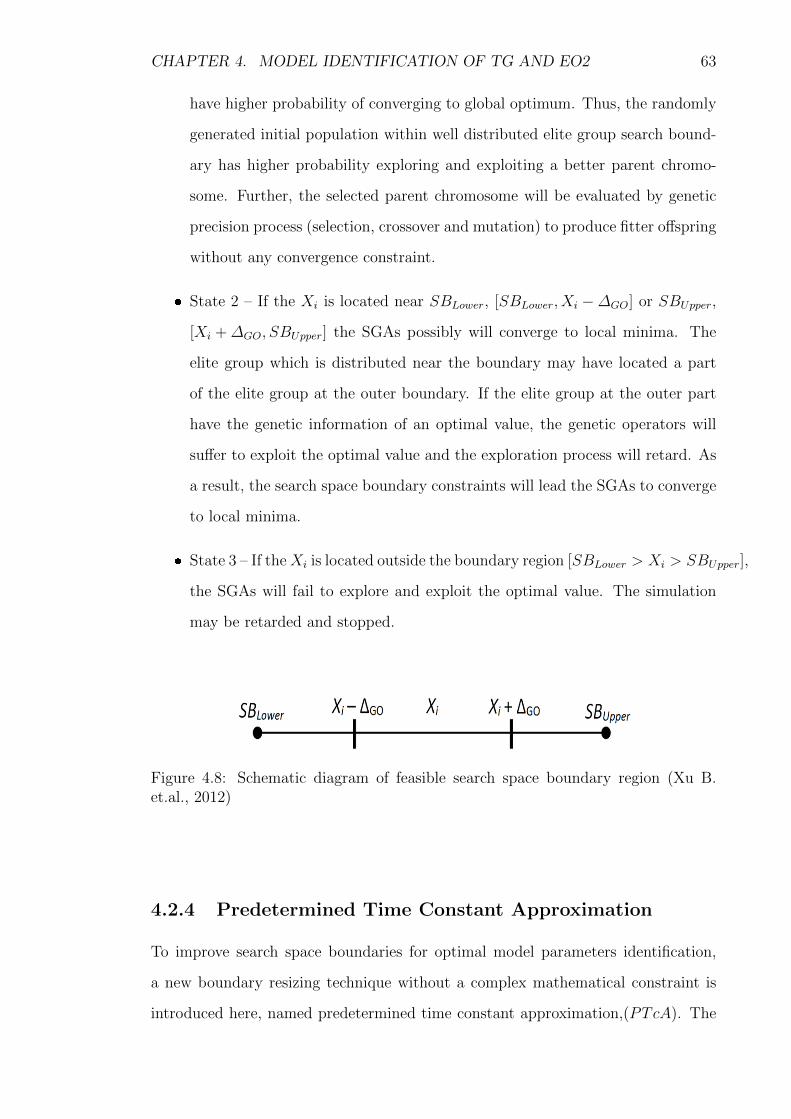
4.8 Schematic diagram of feasible search space boundary region (Xu B.

et.al., 2012) . . . . . . . . . . . . . . . . . . . . . . . . . . . . . . . . 63

ix

LIST OF FIGURES x

4.9 Sub-process of Tsp(Initial) identification from dynamic response . . . . 65

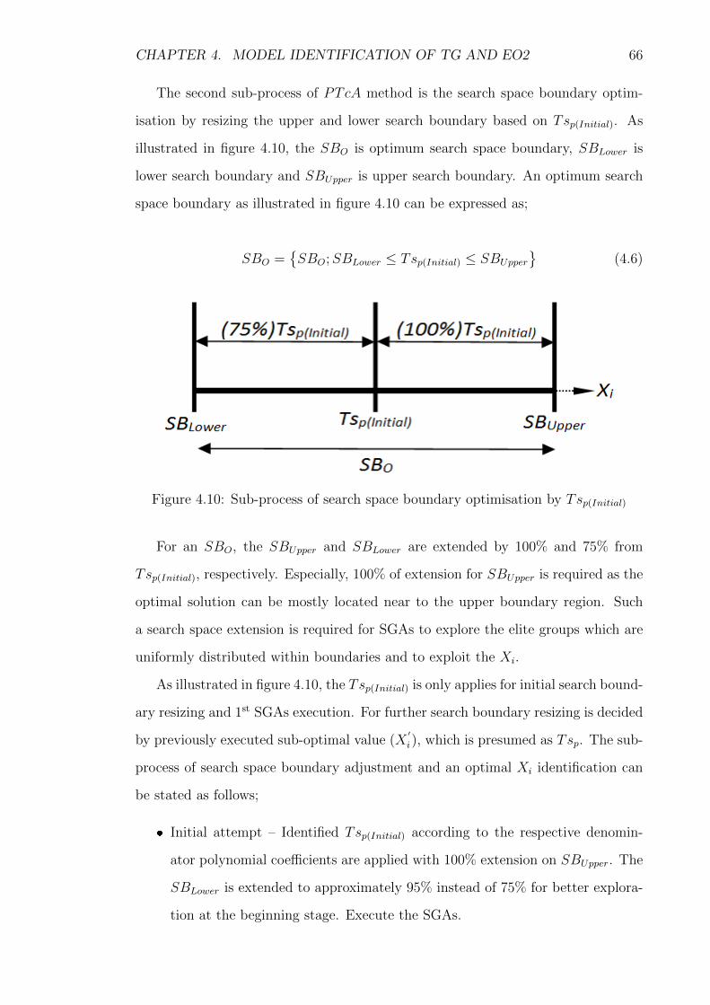
4.10 Sub-process of search space boundary optimisation by Tsp(Initial) . . . 66

4.11 The principle scheme of SGAs for model parameters estimation (Vladu

E. E., 2003) . . . . . . . . . . . . . . . . . . . . . . . . . . . . . . . . 70

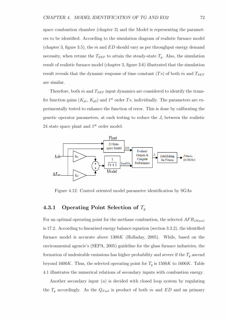
4.12 Control oriented model parameter identification by SGAs . . . . . . 72

4.13 Transient responses of Tg real plant with open-loop technique and

three tuning of SGAs . . . . . . . . . . . . . . . . . . . . . . . . . . 78

4.14 Step response of real industry response of EO2 . . . . . . . . . . . . 79

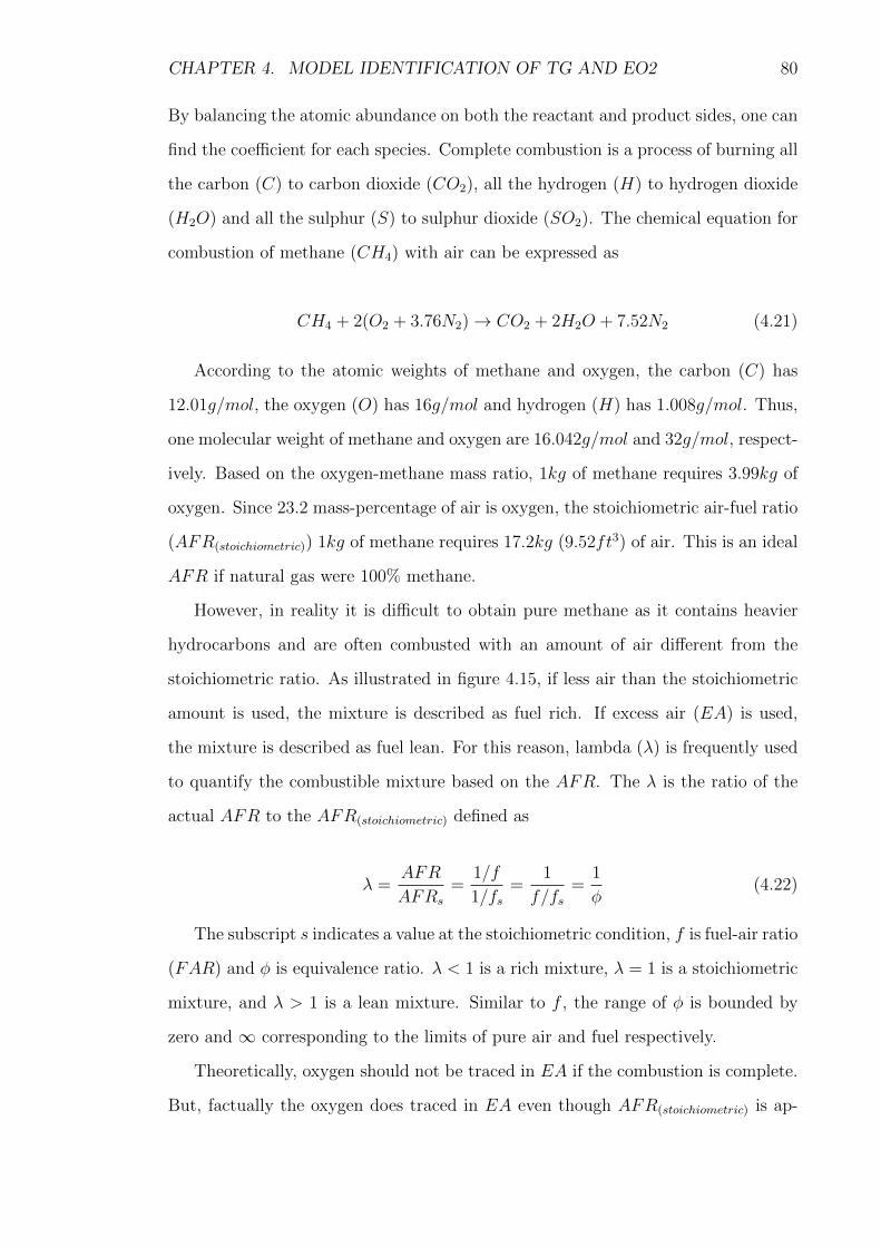
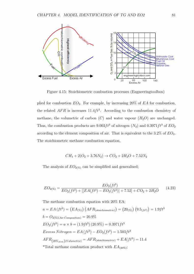
4.15 Stoichiometric combustion processes (Engneeringtoolbox) . . . . . . 81

4.16 Insignificant nonlinear effect of AFR(stoichiometric)(ft3) Vs EO2(%) . . . 83

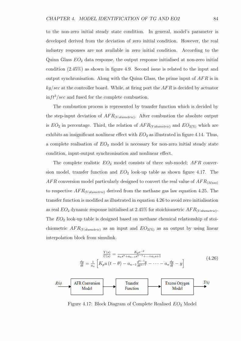
4.17 Block Diagram of Complete Realised EO2 Model . . . . . . . . . . . 84

4.18 Realistic EO2 model set-up for parameter identification . . . . . . . . 86

4.19 Control oriented EO2 model set-up for parameter identification . . . 86

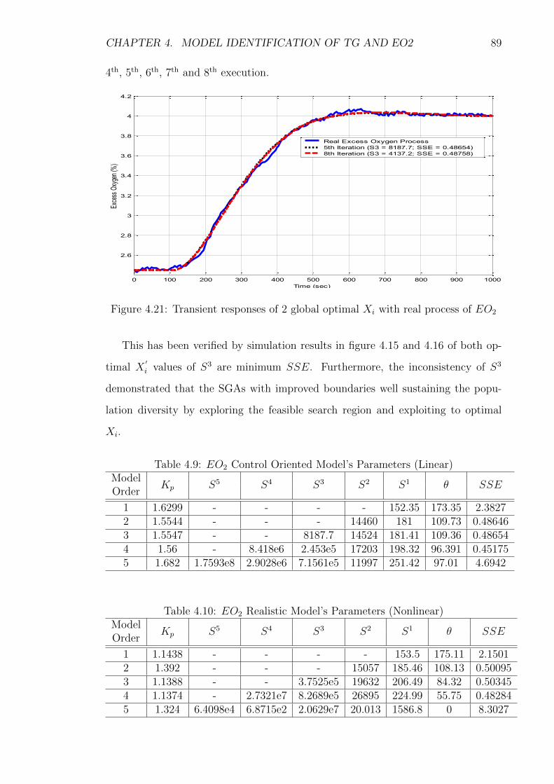
4.20 Two global optima of Xi values of S3 for EO2 . . . . . . . . . . . . . 88

4.21 Transient responses of 2 global optimal Xi with real process of EO2 . 89

4.22 Control oriented (Linear) and realistic (Nonlinear) model orders with

respective SSE . . . . . . . . . . . . . . . . . . . . . . . . . . . . . . 92

4.23 Selected Models Order for Realistic and Control Oriented Models . . 94

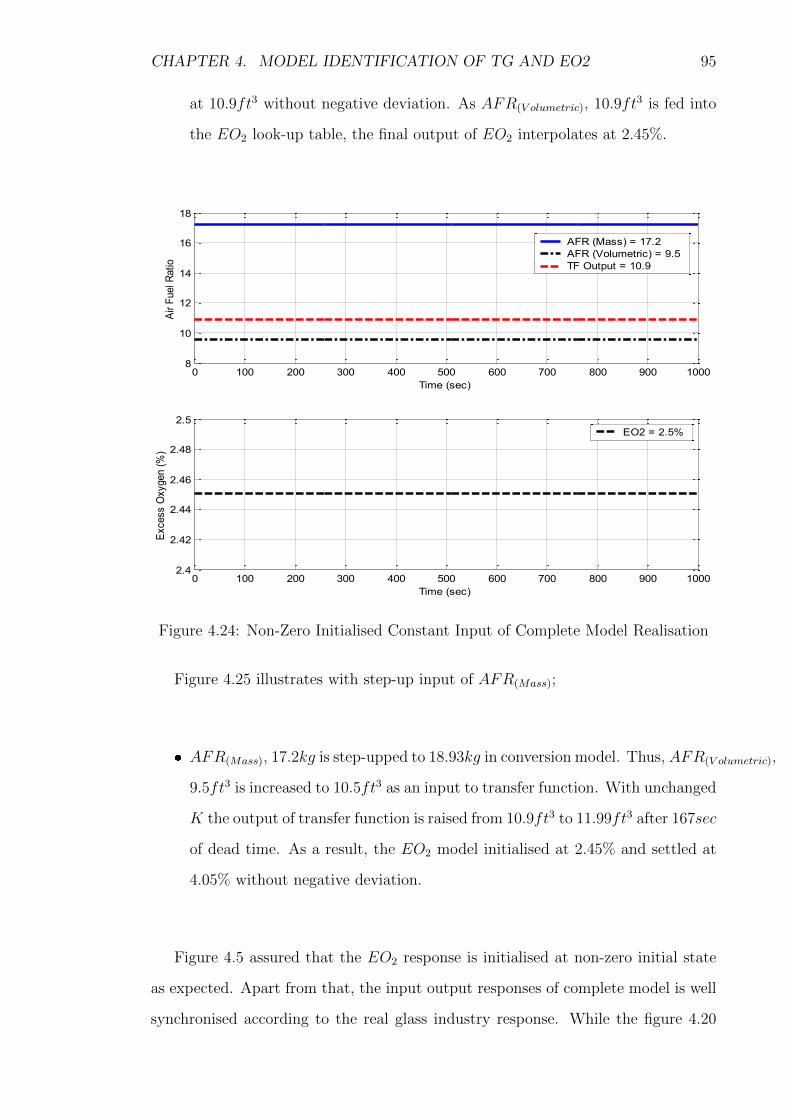
4.24 Non-Zero Initialised Constant Input of Complete Model Realisation . 95

4.25 Non-zero Initialised Step Responses of Identified EO2 Models . . . . 96

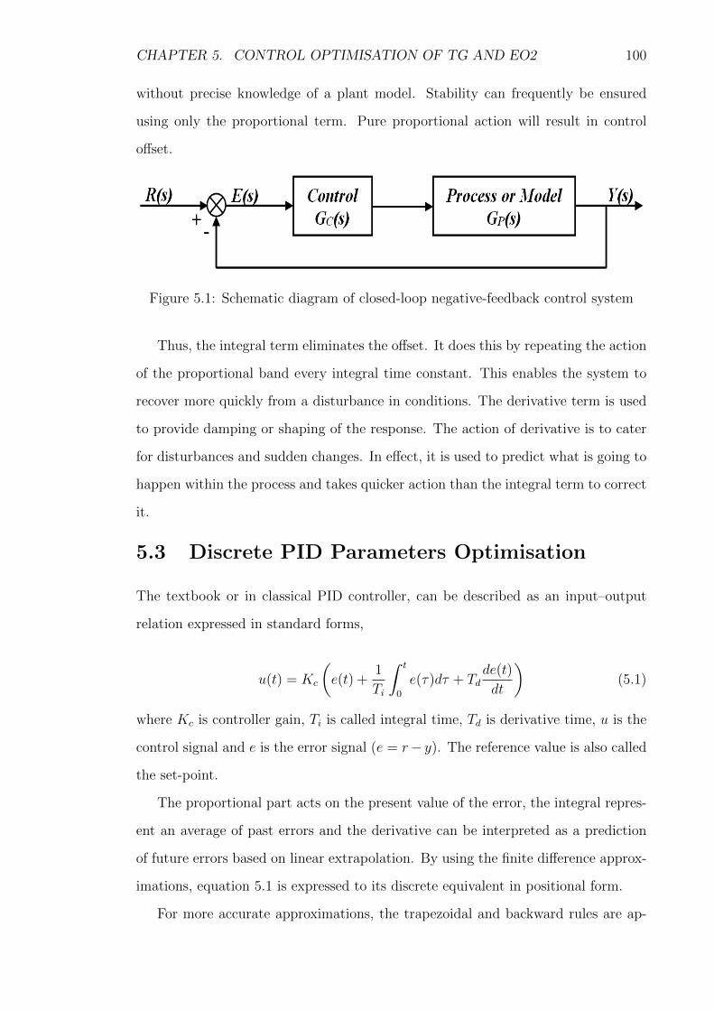
5.1 Schematic diagram of closed-loop negative-feedback control system . . 100

5.2 Flow chart of discrete PID control parameters optimisation by SGAs

(Saad et. al., 2012) . . . . . . . . . . . . . . . . . . . . . . . . . . . . 102

5.3 Wide range of search space boundary responses with respective con-

trol oriented models by SGA’s . . . . . . . . . . . . . . . . . . . . . . 106

5.4 1st order control oriented EO2 model responses; ZN, DS and SGAs

improved search space boundaries . . . . . . . . . . . . . . . . . . . . 108

5.5 2nd order control oriented EO2 model responses; ZN, DS and SGAs

improved search space boundaries . . . . . . . . . . . . . . . . . . . . 108

LIST OF FIGURES xi

5.6 EO2 improved boundaries responses of 1st and 2nd orders control ori-

ented linear models by SGA’s . . . . . . . . . . . . . . . . . . . . . . 109

5.7 Improved boundaries and λ of Tg responses by SGA’s with conven-

tional techniques . . . . . . . . . . . . . . . . . . . . . . . . . . . . . 110

5.8 Effect of P−term and I−term with λ of modified objective function,

IAE + λISU . . . . . . . . . . . . . . . . . . . . . . . . . . . . . . . 112

5.9 Integral output of IAE + λISU objective function with λ = 100 →

850 for Tg . . . . . . . . . . . . . . . . . . . . . . . . . . . . . . . . . 112

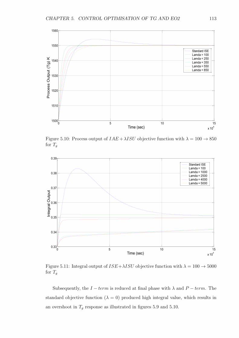
5.10 Process output of IAE+λISU objective function with λ = 100→ 850

for Tg . . . . . . . . . . . . . . . . . . . . . . . . . . . . . . . . . . . 113

5.11 Integral output of ISE + λISU objective function with λ = 100 →

5000 for Tg . . . . . . . . . . . . . . . . . . . . . . . . . . . . . . . . 113

5.12 Process output of ISE + λISU objective function with λ = 100 →

5000 for Tg . . . . . . . . . . . . . . . . . . . . . . . . . . . . . . . . . 114

5.13 Integral output of IAE+λIS∆U objective function with λ = 100→

500000 for Tg . . . . . . . . . . . . . . . . . . . . . . . . . . . . . . . 114

5.14 Process output of IAE + λIS∆U objective function with λ = 100→

500000 for Tg . . . . . . . . . . . . . . . . . . . . . . . . . . . . . . . 115

5.15 Integral output of ISE+λIS∆U objective function with λ = 100→

500000 for Tg . . . . . . . . . . . . . . . . . . . . . . . . . . . . . . . 116

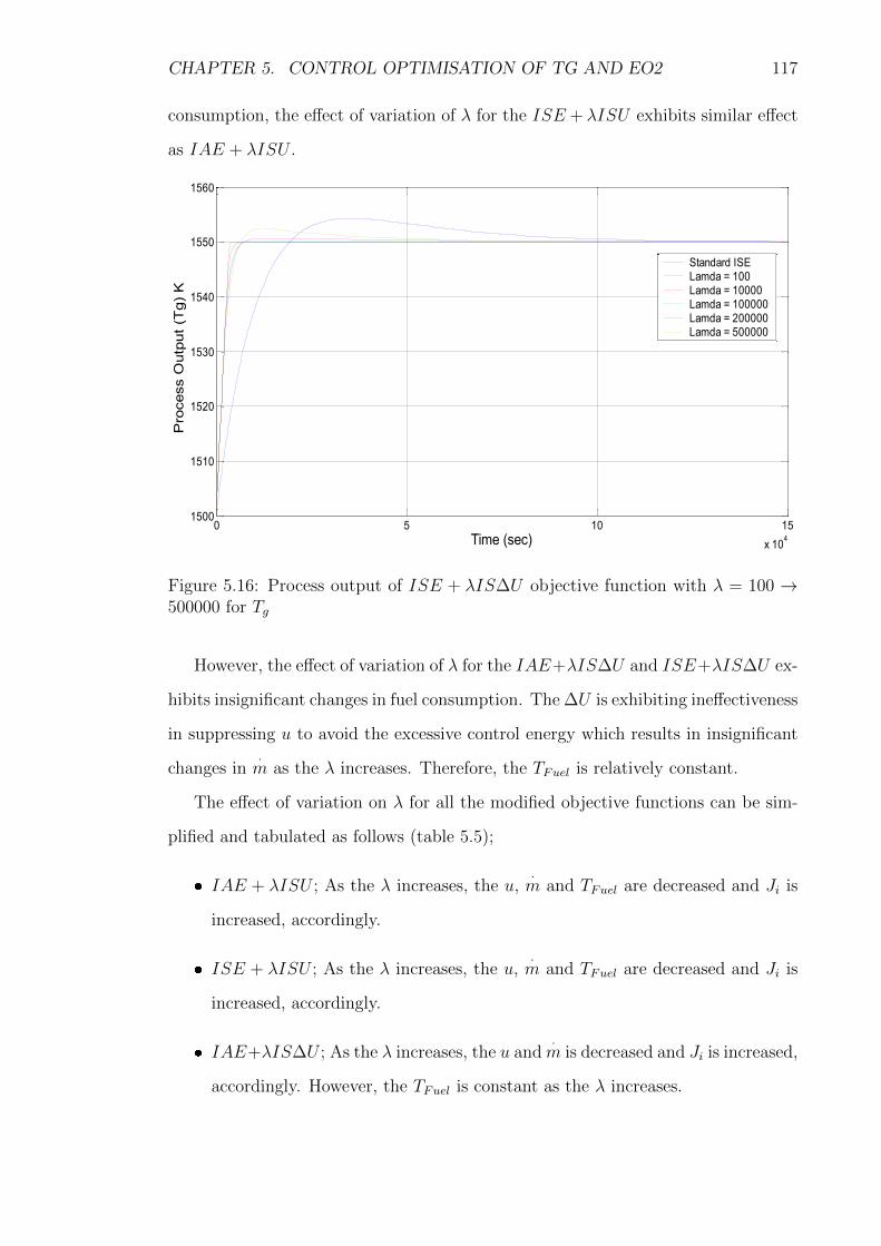
5.16 Process output of ISE + λIS∆U objective function with λ = 100→

500000 for Tg . . . . . . . . . . . . . . . . . . . . . . . . . . . . . . . 117

6.1 2-input, 2-output (TITO) multivariable control oriented model under

closed-loop discrete decentralised PID controllers . . . . . . . . . . . 121

6.2 Transient responses of 1st order control oriented model of EO2 by

three SGAs tuning approaches . . . . . . . . . . . . . . . . . . . . . . 126

6.3 Transient responses of Tg with single-loop interaction by 2nd order

control oriented model of EO2 by three SGAs tuning approaches . . . 126

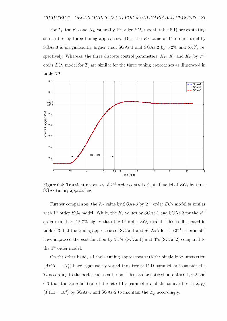
6.4 Transient responses of 2nd order control oriented model of EO2 by

three SGAs tuning approaches . . . . . . . . . . . . . . . . . . . . . . 127

LIST OF FIGURES xii

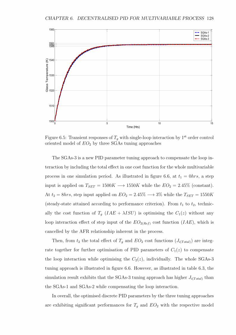
6.5 Transient responses of Tg with single-loop interaction by 1st order

control oriented model of EO2 by three SGAs tuning approaches . . . 128

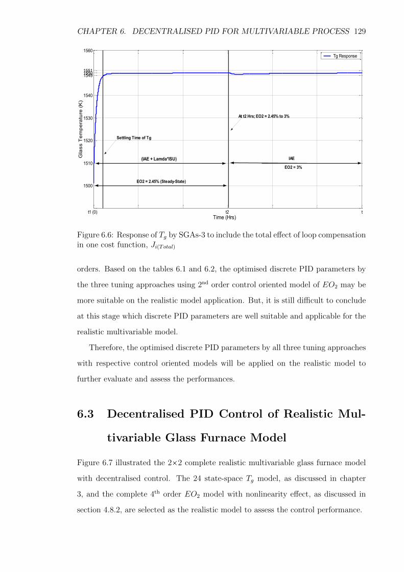
6.6 Response of Tg by SGAs-3 to include the total effect of loop compens-

ation in one cost function, Ji(Total) . . . . . . . . . . . . . . . . . . . 129

6.7 2-input, 2-output (TITO) realistic multivariable model under closed-

loop discrete decentralised PID control . . . . . . . . . . . . . . . . . 130

6.8 Comparison of EO2 control responses on 4th order nonlinear realistic

model . . . . . . . . . . . . . . . . . . . . . . . . . . . . . . . . . . . 131

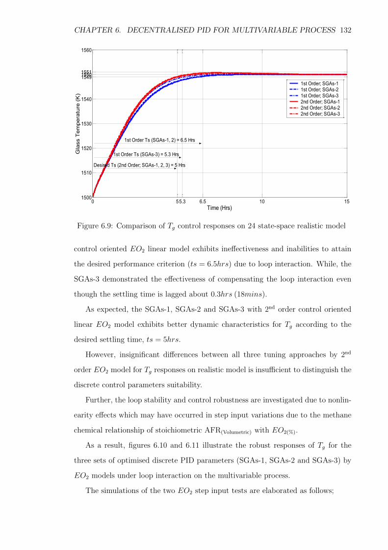
6.9 Comparison of Tg control responses on 24 state-space realistic model 132

6.10 Tg responses under loop interaction of multivariable process by 1st

order EO2 model’s discrete PID parameters (∆1%(AFR)) . . . . . . . 133

6.11 Tg responses under loop interaction of multivariable process by 2nd

order EO2 model’s discrete PID parameters (∆1%(AFR)) . . . . . . . 134

6.12 Fuel consumption under loop interaction of realistic multivariable pro-

cess by 1st order EO2 model’s discrete PID parameters (∆1%(AFR)) . 136

6.13 Fuel consumption under loop interaction of realistic multivariable pro-

cess by 2nd order EO2 model’s discrete PID parameters (∆1%(AFR)) . 137

6.14 Comparison of steady-state of Tg responses by two set-points of EO2 138

7.1 An extension of 24 state-space combustion chamber models to multistage149

7.2 2 Energy Distributions(1350K(Chamber1) −→ 1500K(Chamber2)),(1400K(Chamber1) −→

1500K(Chamber2)) . . . . . . . . . . . . . . . . . . . . . . . . . . . . . 180

7.3 2 Energy Distributions(1450K(Chamber1) −→ 1500K(Chamber2)),(1500K(Chamber1) −→

1550K(Chamber2)) . . . . . . . . . . . . . . . . . . . . . . . . . . . . . 181

List of Tables

2.1 Comparison of the deterministic techniques . . . . . . . . . . . . . . . 14

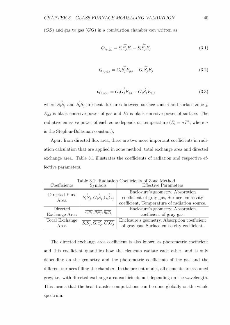
3.1 Radiation Coefficients of Zone Method . . . . . . . . . . . . . . . . . 40

3.2 24 State-space Variables of the Simulated Furnace Model . . . . . . . 46

4.1 Selection of Operating Point of Tg and u with AFR(Mass) (17.2) . . . 73

4.2 Selected genetic operators of Tg . . . . . . . . . . . . . . . . . . . . . 74

4.3 Model Parameters Identification by SGAs1 Execution . . . . . . . . . 77



4.6 AFR(stoichiometric)with relative EA and EO2 . . . . . . . . . . . . . . 83

4.7 Selected genetic operators of EO2 . . . . . . . . . . . . . . . . . . . . 85

4.8 3rd Order Model Polynomial Coefficient Approximation by SGAs Ex-

ecution . . . . . . . . . . . . . . . . . . . . . . . . . . . . . . . . . . . 88

4.9 EO2 Control Oriented Model’s Parameters (Linear) . . . . . . . . . . 89

4.10 EO2 Realistic Model’s Parameters (Nonlinear) . . . . . . . . . . . . . 89

4.11 Information Criterion of Model Orders . . . . . . . . . . . . . . . . . 91

4.12 Roots of Denominator of Model Orders . . . . . . . . . . . . . . . . . 93

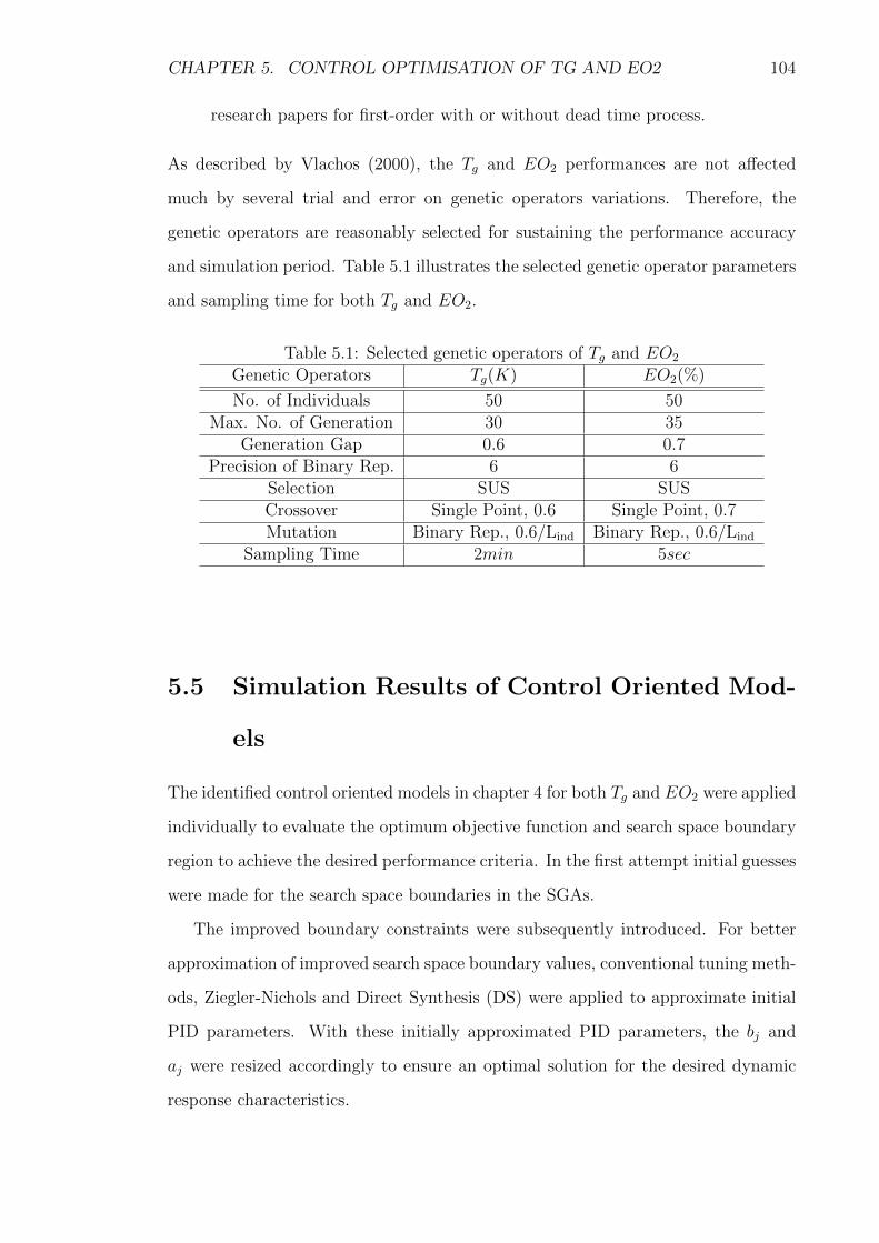
5.1 Selected genetic operators of Tg and EO2 . . . . . . . . . . . . . . . . 104

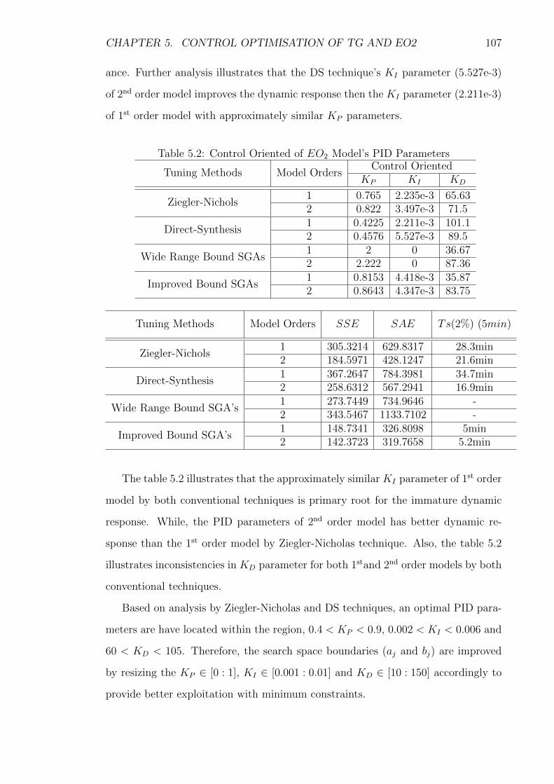
5.2 Control Oriented of EO2 Model’s PID Parameters . . . . . . . . . . . 107

5.3 PID parameters for control oriented Tg by different tuning methods . 110

5.4 Weighting factor identification with IAE + λISU . . . . . . . . . . . 111

5.5 Effect of λ variations for the modified objective functions . . . . . . . 118

xiii

LIST OF TABLES xiv

6.1 Identified PID parameters for Tg and 1st order control oriented model

of EO2 by three SGAs tuning approaches . . . . . . . . . . . . . . . 125

6.2 Identified PID parameters for Tg and 2nd order control oriented model

of EO2 by three SGAs tuning approaches . . . . . . . . . . . . . . . 125

6.3 Error criteria with respective cost function by three SGAs tuning

approaches . . . . . . . . . . . . . . . . . . . . . . . . . . . . . . . . 125

6.4 Fuel consumption for multivariable process by 2% of EO2 reduction . 135

6.5 Simulation result of fuel consumption by 2% EO2(Ref) reduction . . . 140

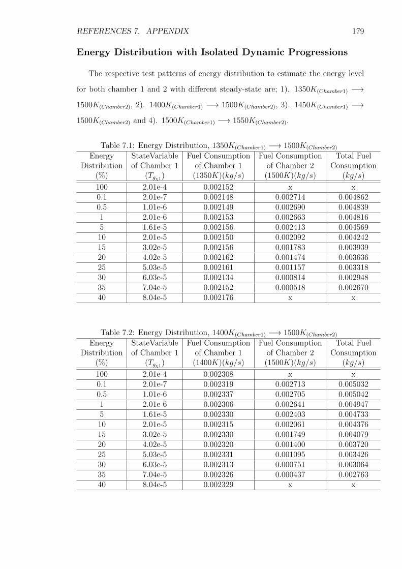
7.1 Energy Distribution, 1350K(Chamber1) −→ 1500K(Chamber2) . . . . . . 179




Glossary of Symbols

Nomenclature

α1 Gas flame zone

α2 Gas non-flame zone

β1 Glass surface flame zone (half inch thickness)

β2 Glass surface non-flame zone (half inch thickness)

∆GO Genetic operator for convergence precision

δ1 Glass volume flame zone (bottom half)

δ2 Glass volume non-flame zone (bottom half)

δ(%) Settling band

εg Emissivity coefficient of real gas

ζ Zeta, damping ratio

θi Angle of surface elements, i

θj Angle of surface elements, j

k Emissivity coefficient of gas

λ Lambda, weighting factor, combustible mixture

ρ Density

σ Stephan-Boltzman constant

φ Equivalent ratio combustible mixture

χ1 Glass volume flame zone (top half)

χ2 Glass volume non-flame zone (top half)

ωn Natural frequency

ωpc Phase crossover frequency

Ai Area of surface element i

xv

GLOSSARY OF SYMBOLS xvi

Aj Area of surface element j

an...a1 Coefficients of denominator polynomials

ag Gray gases

aj Lower boundary of individual chromosome’s

a Time constant

bj Upper boundary of individual chromosome’s

Ci Constant by set of initial conditions

Css Zero steady-state

c Specific heat

Dec Decimal value of respective binary string

Ei Black emissive power of surface i

Ej Black emissive power of surface j

E(s) Control error

Eg,i Black emissive power of gas

f Fuel-air ratio

fs Stoichiometric fuel-air ratio

f1 Algebraic expression of fuel controller (kg/s)

f2 Algebraic expression of thermal energy demand (K)

f(t− θ) Input signal or forcing function with time delay

GC(s) Control strategies

Gi Heat flux gas zone i

Gj Heat flux gas zone j

GP (s) System’s process

h Radiation heat transfer coefficient

Ji Performance criterion

KD Derivative gain

KI Integral gain

K Number of parameters

Kp Process gain

KP Proportional gain

GLOSSARY OF SYMBOLS xvii

.m Fuel flow (kg/s)

.m Fuel flow (kg/s)

Maxfuel(constant) Maximum fuel flow (constant) (kg/s)

mj Number of bits of individual chromosome’s

n Sample size

Pf Internal pressure of furnace (psi)

Pi Incident power

pi Root of denominator

P Partial pressure of gray gases

Q Generated heat

QiG,jG Heat transfer between gas zone i and gas zone j

QiG,jS Heat transfer between gas zone i and surface zone j

QiS ,jS Heat transfer between surface zone i and gas surface j

qrad, Net rate of heat flow

q Power loss

QFuel Pressurised fuel flow as energy

R Methane gas constant (ft.Ibf/Ibm.R)

R(s) Reference input

rij Size of vector that connects the centres of two elements

Si Heat flux surface zone i

Sj Heat flux surface zone j

T1, T2 Absolute temperature of involved regions

ts Settling time

t Time

u Temperature feedback error

V Mean methane temperature (K).

V Methane flow rate in volumetric (ft3/hr)

Vi Volume of gas element i

Vj Volume of gas element j

Xi Optimal value

xj Respective real value of the chromosome’s

GLOSSARY OF SYMBOLS xviii

X′i Sub-optimal value

Y (s) Controlled output

Y outN(t) Model process output signal

y(t) Output Signal

Y (t) Real process output signal

Abbreviations

AFR Air-fuel ratio

AFR(Mass) Air-fuel ratio in mass (kg)

AFRstoichiometric) Stoichiometric Air-fuel ratio

AFR(V olumetric) Air-fuel ratio in volumetric (ft3)

AIC Akaike information criterion

AICc Akaike information criterion with correction

BIC Bayesian information criterion

BLT Biggest log modulus

C Carbon

CFD Computational fluid dynamics

Cg Glass temperature control

CH4 Methane fuel

CO2 Carbon dioxide

DCSs Distributed Control Systems

DRP Process’s dynamic period

DS Direct-Synthesis

EA Excess air

ED Thermal energy demand (K)

EO2 Excess oxygen (%)

EOP Effective open-loop

FOPDT First-order plus dead-time

FPE Akaike’s Final prediction error criterion

GM Gain Margin

GLOSSARY OF SYMBOLS xix

H Hydrogen

H2O Hydrogen oxide (Water)

IAE Integral absolute error

IMC Internal model control

ISE Integral sum error

LHV Lower calorific heat value (MJ/kg)

MIMO Multiple-input multiple-output

MOEA Multi-objective evolutionary algorithm

MRAC Model reference adaptive control

N2 Nitrogen

O2 Oxygen

PID Proportional, Integral, Derivative

PLC Programmable Logic Controllers

POD Proper orthogonal decomposition

PSO Particle swarm optimiser

PTcA Predetermined time constant approximation

RETF Reduced effective transfer function

RGA Relative gain array

S Sulphur

SAE Sum of absolute error

SBLower Lower search boundary

SBO Optimum search boundary

SBUpper Upper search boundary

SGAs Standard genetic algorithms

SISO Single-input single-output

SO2 Sulphur dioxide

SOPDT Second-order plus dead-time

SSE Sum of square error

Tamb Ambient temperature (K)

Tg Glass temperature (K)

Tsp(Initial) Initial predetermined time constant

GLOSSARY OF SYMBOLS xx

TITO Two-input two-output

TSET Primary temperature setting (K)

Algorithm Definitions

FitnV Fitness value, chromosomes evolution

Ggap Generation gap

Lind Length of chromosome

Nind Number of individuals

Nkeep Number of selected group of fitter chromosomes

Nkeep1 Offspring chromosomes matrix of new population

Npop Number of population size

Nva Number of variables

PRECI Precision, number of bits depends on desired accuracy

SEL− F Selection function

Srate Selection rate, fraction of number of population

SUS Stochastic universal sampling, selection process

XOV − F Crossover function

Xrate Probability of recombination rate

Chapter 1

INTRODUCTION – OVERVIEW

AND THESIS OUTLINE

This chapter begins with a brief review of the obstacles faced in glass furnace in-

dustries to optimise the desire performances. In particular, the tight environmental

regulations to control undesirable emissions associated with burning fossil fuels and

excess oxygen. Finally, the project scope and the structure of this thesis are outlined.

1.1 Review of Glass Furnace Processes and Con-

trol

Glass manufacturing represents a challenge for automation and for control engin-

eers as it is a very complex, long dynamic process with complicated, nonlinear and

not completely understood dynamical behaviour. So it is still common that glass

furnaces are controlled by simple controllers such as PID regulators or by manual in-

terventions of furnace operators. As a result, the process may be kept in suboptimal

conditions and acting disturbances may not be effectively rejected.

However, market competition creates a need for tighter control of the process

towards optimum. Glass furnaces are usually energised by fossil fuels or electricity.

The massive furnaces with multiple port burners cause the glass manufacturing in-

dustries to consume high energies in glass production. Most glass industries are

1

CHAPTER 1. INTRODUCTION – OVERVIEW AND THESIS OUTLINE 2

operating at maximum daily through-put to fulfil the market demand and require-

ment. High energy costs and severe competition amongst glass manufacturers has

resulted in the emergence of several solutions to reduce the fuel consumption of these

furnaces.

Apart from high energy consumption, undesirable emission from glass industries

is another setback to consider as the entire world is greatly concerned about green

house effects. Tight environmental regulations are now applied to reduce carbon

monoxide, sulphur dioxide, nitrogen oxides and particles that are undesirable emis-

sions associated with burning fossil fuels. These compounds are toxic, contribute to

pollutions and can ultimately cause health problems.

In the USA, federal and state laws govern the permissible emission rates for

these pollutants under the guidance of the Clean Air Act and oversight of the fed-

eral Environmental Protection Agency (EPA), National Risk Management Research

Laboratory, (2004). State and local environmental agencies also exert authority in

regulating the emissions of these pollutants.

Globally, 191 states have signed and ratified the Kyoto Protocol (1998) to ex-

ecute themselves in a reduction of four green-house gases (carbon dioxide, methane,

nitrous oxide and sulphur hexafluoride) which would badly interfere with the global

climate system and human health. According to article 2 of the Kyoto Protocol,

the reduction of emissions is focused on industrial combustion emission. As a result,

the industries which are related to combustion processes are tightly observed by

environmental agencies to ensure stabilization of green house gases emission.

To act in accordance with emission guidelines and for clean emission, most

process industries are emphasising in reduction of the excess oxygen (EO2) by

controlling the air-fuel ratio (AFR). EO2 is an important element in combustion

products that would lead to formation of sulphur dioxide (SO2) and nitrous oxide

(NO2). According to the combustion emission guideline, the permissible EO2 is not

more than 3% from combustion, excluding Japan which allows not more than 5%

of EO2 from combustion.


1.2 Problem Statement

Literature survey reveals that there has been no research undertaken on EO2

model parameter identification and control parameter optimisation. Also, an insig-

nificant number of works has been undertaken on control parameter optimisation

for glass furnaces. Further, the glass and other process industries generally operate

within emission guidelines which are regulated by environmental agencies (SEPA,

2005). Thus, a necessity of an EO2 model parameters identification has not arisen

and has not been considered. However, at maximum operating conditions with high

energy consumption, the probability of producing undesirable emission is high. Any

occurrence of sudden undesirable disturbances can cause more problems for existing

furnaces which are operating in poor thermal conditions.

Therefore, it is clear that in order to bridge the gap between EO2 and the

glass furnace, a multivariable process with the respective discrete control parameters

will be designed to minimise the fuel consumption while sustain the desired glass

temperature. The research presented in this thesis is focused on this problem and

delivers solutions that satisfy these criteria.

1.3 Research Novelty and Methodology

The primary endeavour of this research is to design a multivariable glass furnace

model for fuel consumption minimization and EO2 reduction while sustaining the

desired output. The strategy of this work is developed using standard genetic al-

gorithms (SGAs), a heuristic optimisation technique based on Darwin’s theory 1.

The developed models and control methods will be evaluated applying simulation

and Matlab software.

More specifically, this thesis addresses the distinct objectives below and as de-

1

Darwin’s theory of biological evolution, stating that all species of organisms arise and develop

through the natural selection of small, inherited variations that increase the individual’s ability to

compete, survive and reproduce


Figure 1.1: Schematic Flow of Research Methodology

scribed in schematic flow (Figure 1.1):

1. Identify and investigate the dynamic characteristics of a realistic 24 state-

space glass temperature (Tg) model. Then, develop a control oriented glass Tg

simulation model.

2. Develop and investigate a realistic simulation model with nonlinear effect and

a control oriented simulation model without nonlinear effect of excess oxygen

(EO2) from numerical data of real plant.

3. Optimise the discrete control parameters according to the performance criteria

of Tg and EO2, individually.

4. Develop the discrete decentralised control strategies by control oriented models

of Tg and EO2. Then, improve and optimise the dynamic discrete control

strategies by three tuning approaches.


5. Implement and evaluate the optimised discrete control strategies on realistic

multivariable process for attaining the desired performances.

1.4 Thesis Outline

The structure of this thesis is outlined below. Most of the material contained in

chapters 2 and 3 is standard and is only intended as a brief review of the current

state of affairs in the field of GAs as function optimisers. The main contributions

and novel aspects of this work are contained in chapters 4 to 6 and are summarised

in Chapter 7.

� Chapter 2 - Literature Review of Standard Genetic Algorithms

This chapter commences with a brief overview of optimisation algorithms as ap-

plied to the solution of control engineering problems. Standard Genetic Algorithms

(SGAs) as function optimisers are then introduced, focusing on their fundamental

differences and advantages over conventional algorithms. The relevance of SGAs to

control systems is then illustrated by a number of successful applications in different

areas of process modelling and control optimisation. Finally, applications of SGAs

for glass furnace and furnace type processes are outlined.

� Chapter 3 - Review of Glass Furnace Modelling

This chapter begins with a brief literature review of designing the combustion cham-

ber, which is fundamental to the developed methods for the glass furnace models.

Computational fluid dynamics method derived from radiative heat transfer were ap-

plied here to analyse the temperature distribution within the combustion chamber,

which is divided into finite zones. Linearised energy balance equations in steady-

state improve the prediction and accuracy of temperature distribution within finite

zones. An assessment on the selected glass furnace model, which is designed by a

zone method, provides a deeper insight of model understanding and quantitative

performance.


� Chapter 4 - Model Parameters Identification of Glass Temperature

and Excess Oxygen

This chapter is primarily focused on optimal control oriented model’s parameter

identification for glass temperature and excess oxygen. A common phenomenon of

premature convergence, which is the search space constraint, in SGAs is reviewed. A

novel technique, predetermined time constant approximation, is proposed to enhance

the search mechanism to optimise the search boundaries to locate optimal values

of model parameters. Further, a full scale realistic excess oxygen model which

consists of air-fuel ratio conversion model, dynamic transfer function model and

excess oxygen look-up table, is developed by using a real plant’s numerical data of

excess oxygen.

According to the literature survey, there is no realistic excess oxygen model

available for further research. Therefore, the development of a realistic excess oxygen

model is essential for further research here. Also, control oriented models of both

glass temperature and excess oxygen processes are developed for control parameter

optimisation.

� Chapter 5 - Control Parameters Optimisation of Glass Temperat-

ure and Excess Oxygen

In this chapter, the discrete control (PID) parameters optimisation by SGAs for

control oriented models of glass temperature and excess oxygen, which are identified

in chapter 4, is primarily focused on. A literature review of PID control strategies

and tuning issues are briefly discussed and addressed. The control parameters of

both control oriented models are optimised individually without loop interaction

according to the desired performance criteria. The improved search space boundaries

and modified objective function are subsequently introduced for excess oxygen and

glass temperature respectively, to improve the discrete PID parameters to attain the

desired dynamic performance criteria.

The search space boundaries are improved by resizing the upper and lower bound-

aries with an assist of conventional tuning techniques, Ziegler-Nichols and Direct


Synthesis, for an initial knowledge of PID parameters. For the glass temperature,

the objective function is modified by adding a weighting factor with input term to

achieve the desired characteristic response. Further, three other modified objective

functions are analysed and compared with the selected objective function for better

dynamic characteristics of glass temperature response.

� Chapter 6 - Decentralised PID Controller Tuning for Multivariable

Glass Furnace Process

In this chapter, the decentralised discrete PID control tuning techniques are investig-

ated for the multivariable glass furnace process. A literature review of multivariable

PID control strategies and tuning issues are briefly discussed and addressed. Three

tuning approaches with respective objective functions are investigated to optimise

the control performances for control oriented multivariable glass furnace models. An

improved and modified objective function which includes the total effect is proposed

with other conventional tuning techniques, based on SGAs. This modified objective

function is shown to exhibit improved control robustness and disturbance rejection

under loop interaction. This is achieved by combining both optimal objective func-

tions of Tg and EO2 on control oriented models which were developed individually

in chapter 5.

Further, the set of discrete PID parameters are applied on the multivariable

realistic model of Tg and EO2 to optimise fuel consumption reduction and excess

oxygen while sustaining the glass temperature. Simulation results are presented to

illustrate the effectiveness of the proposed method.

� Chapter 7- Conclusions - Main Contributions and Further Work

The first part of this chapter summarises the key results and main contributions of

this research project. A number of recommendations for further work in this direc-

tion, which will extend an improvement of SGAs in the area of model parameters

identification and state-space model extension with respective thermal energy as

input, are given in the second part of this chapter.


1.5 Dissemination of Research Contributions

During this research an endeavour has been made in order to suggest the ideas and

methodologies proposed in this thesis to a variety of different audiences through both

peer reviewed publications and presentations. The publications made throughout

the duration of research are listed below:

� Rajarathinam K., Gomm J. B. and Yu D. L, “Identification, Simulation and

Control Optimisation of a Glass Furnace by Genetic Algorithm”, Proceeding

of the GERI 8th Annual Research Symposium (GARS 2013), LJMU, UK, 2013,

� Rajarathinam K., Gomm J. B., Yu D. L. and Abdelhadi A. S., “Minimisation

of Fuel Consumption in a Glass Furnaces Industry by Standard Genetic Al-

gorithms”, Proceeding of the GERI 9th Annual Research Symposium (GARS

2014), LJMU, UK, 2014.

� Rajarathinam K., Gomm J. B., Yu D. L. and Abdelhadi A. S., “Decent-

ralised Control Optimisation for a Glass Furnace by SGA’s”, Proceeding of

the 15th International Conference on Computer Systems and Technologies

(CompSysTech’14), Ruse, Bulgaria, 2014. Also published in ACM Interna-

tional Conference Proceeding Series, vol. 883, pp. 248-255, 2014. (Best Paper

Award)

� Rajarathinam K., Gomm J. B., Yu D. L. and Abdelhadi A. S., “Decentralised

PID Control Tuning for a Multivariable Glass Furnace by Genetic Algorithm”,

Proceeding of the 20th International Conference on Automation and Comput-

ing (ICAC), Bedfordshire, UK, pp. 14-19, 2014.

� Rajarathinam K., Gomm J. B., Yu D. L. and Abdelhadi A. S., “PID Control-

ler Tuning for a Multivariable Glass Furnace Process by Genetic Algorithm”,

International Journal of Automation and Computing (IJAC), vol. 13 (1), pp.

64-72, 2016. (accepted, June 2015).

� Rajarathinam K., Gomm J. B., Yu D. L. and Abdelhadi A. S., “Predetermined

Time Constant Approximation Method for Model Identification Search Space


Boundary by Standard Genetic Algorithm”, SIAM Conference on Control and

Its Applications, Paris, France, CP22, pp. 73, 2015. (Abstracts accepted).

� Rajarathinam K., Gomm J. B. and Yu D. L., “Predetermined Time Constant

Approximation Method for Optimising Search Space Boundary by Standard

Genetic Algorithm”, Proceeding of the 16th International Conference on Com-

puter Systems and Technologies (CompSysTech’15), Dublin, Ireland, 2015.

Also published in ACM International Conference Proceeding Series, vol. 1008,

pp. 38-45, 2015.

� Rajarathinam K., Gomm J. B., Yu D. L. and Abdelhadi A. S., “An Improved

Search Space Resizing Method for Model Identification by Standard Genetic

Algorithm”, Proceeding of the 21st International Conference on Automation

and Computing (ICAC), Glasgow, UK, pp. 1-6, 2015.

This chapter begins with an overview of challenges that are face by glass furnace in-

dustries in higher fuel consumption and undesirable emission. The research method-

ologies and the structure of this thesis are outlined, and related research publications

are listed.

Chapter 2

Literature Review of Optimisation

and Genetic Algorithms

2.1 Introduction

This chapter commences with a brief overview of optimisation algorithms as ap-

plied to the solution of control engineering problems. Standard Genetic Algorithms

(SGAs) as function optimisers are then introduced, focusing on their fundamental

differences and advantages over conventional algorithms. The relevance of SGAs to

control systems is then illustrated by a number of successful applications in differ-

ent areas of process modelling, control optimisation, multiobjective optimisation and

the negative aspect of optimisation by premature convergence factors are reviewed.

Further, the single-input single-out and multi-variable PID tuning strategies are re-

viewed. Finally, applications of SGAs for glass furnace and furnace type processes

are outlined.

2.2 Definition of Optimum

In general, an optimisation is applied to locate the finest promising solutions to a

specified difficulty. In the simplest case, an optimisation problem consists of maxim-

ising or minimising an objective function, Ji, by systematically selecting the input

variables from within a feasible parameter set depending on the desired criterion.

10

CHAPTER 2. LITERTURE REVIEW OF OPTIMISATION AND GAS 11

The generalization of optimization theory and techniques to other formulations com-

prises a large area of control theory or applied mathematics.

In mathematics, maxima and minima are the prime values (maximum) or least

values (minimum) that a function brought in a point either within a given local

minima or on the function domain in its global maximum. Figure 2.1 illustrates the

local and global maxima and minima for a random function, f(x) = exp−x.cos(2πx)

for 0.2 ≤ x ≤ 2.7.

0 0.5 1 1.5 2 2.5 3

-0.8

-0.6

-0.4

-0.2

0

0.2

0.4

0.6

Global Maxima

Local Maxima

Global Minima

Local Minima

Figure 2.1: Global and local maxima and minima

Furthermore, the classification of an optimal solution is problem dependent. For

instance, single objective optimisation can be classified either minimum or max-

imum. Whereas, for multi objective optimisations minimum or maximum percep-

tions are rather applied to sets F consisting of n =| F |objective functions fi, each

representing one criterion to be optimised [Kalyanmoy, 2001].

F = {fi : X → Yi : 0 < t < n, Yi ⊆ R} (2.1)

2.3 Overview of Optimisation Algorithms

It is difficult to visualize the selection of existing computational tasks and the number

of algorithms developed to resolve them. In general, the heuristic can be categor-


ised into two groups of techniques; deterministic and probabilistic techniques. The

overview begins with deterministic search algorithm. The straightforward searching

algorithm is known as exhaustive search, which endeavours all potential solutions

from a predetermined set and consequently selects the optimal value.

� Local search is an uncomplicated search technique, however with limited

search space. This technique is constantly examining the current solution and

replacing it if the neighbour’s solution is better than the current one. If the

solution is not improved further, the current solution can be considered as

a local optimal solution [Kokash and Natallia, 2005]. Popular hill-climbing

techniques belong to this class. For instance, heuristics for the problem of

intergroup replication for multimedia distribution service based on Peer-to-

Peer network is based on a hill-climbing strategy [Xiang et. al., 2004].

� Divide & Conquer (D&C) is an algorithm attempt to resolve in effortlessly

by partitioning a problem into sub-problems. Subsequently, the resolution of

the sub-problems should be combinable to provide a resolution to the original

problem. Although this method is an efficient algorithm and applicable for

any problems, the shortcoming is that it is time consuming to comprehend

and design D&C. Also, it is difficult to partition and combine back the sub-

problem in such an approach [Cormen et. al., 2000].

� Branch-and-Bound (B&B) is an algorithm design paradigm for discrete

and combinatorial optimisation problems. This algorithm consists of a sys-

tematic enumeration of candidate solutions by means of state space search,

which the set of candidate solutions is thought of as forming a rooted tree

with the full set at the root. The algorithm explores branches of this tree,

which characterise subsets of the solution set. Before enumerating the can-

didate solutions of a branch, the branch is ensured against upper and lower

estimated bounds on the optimal solution, and is discarded if it cannot pro-

duce a better solution than the best one found so far by the algorithm. But

the B&B algorithm is extremely time-consuming if the numbers of nodes in


branches of the tree are large [Kokash and Natallia, 2005].

� Dynamic programming (DP) is a very influential algorithmic paradigm

in which a problem is solved by identifying a collection of sub-problems and

attempting them one at a time. Then using the solution to sub-problems to

assist solving larger ones, until the whole problem is solved. The key point

for applying this technique is formulating the solution process as a recursion

[Bertsekas, 2000]. The biggest drawback of dynamic programming is that is

time consuming due to dimensionality. In higher dimensions, a generalized

implementation is applied that explicitly checks for legal operators at each

node. This introduces a constant factor to the time complexity of DP since

processing each node takes longer than it would in an implementation tailored

to a specific dimension [Hohwald et. al., 2003].

� Greedy algorithm is perhaps the most uncomplicated and influential method

that is based on the evident principle of taking the (local) best selection at

each stage of the algorithm in order to locate the global optimum of some

objective function. For large complex cases this method is time consuming

and does not always provide the best solution as its only search and select the

best choice from current search state [Cormen et. al., 2000].

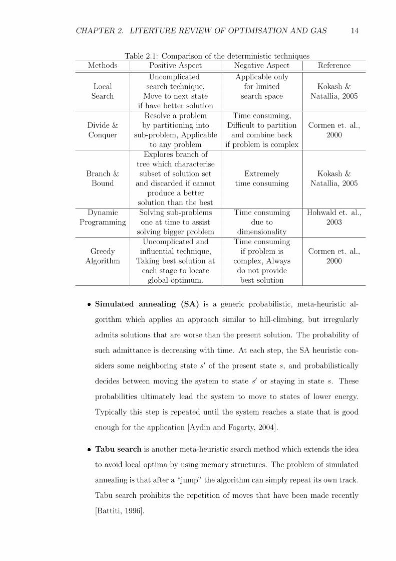
The deterministic heuristic techniques are relatively effective but their time-complexity

often is too high and unacceptable for NP-complete tasks. Also, the deterministic

techniques are tending to premature convergence and generally locate the nearest

local optimum which maybe a low quality. The summary of deterministic heuristic

techniques are tabulated in table 2.1 for comparison.

The purpose of probabilistic heuristics is to overcome these drawbacks. The

comparative studies of probabilistic heuristics are illustrated and simplified in Gamal

et. al., (2014).

� Evolutionary Algorithms (EAs) are succeeding in evading premature con-

vergence by considering a number of solutions simultaneously which will be

discussed more elaborately in the next section.


Table 2.1: Comparison of the deterministic techniquesMethods Positive Aspect Negative Aspect Reference

Uncomplicated Applicable onlyLocal search technique, for limited Kokash &Search Move to next state search space Natallia, 2005

if have better solutionResolve a problem Time consuming,

Divide & by partitioning into Difficult to partition Cormen et. al.,Conquer sub-problem, Applicable and combine back 2000

to any problem if problem is complexExplores branch of

tree which characteriseBranch & subset of solution set Extremely Kokash &

Bound and discarded if cannot time consuming Natallia, 2005produce a better

solution than the bestDynamic Solving sub-problems Time consuming Hohwald et. al.,

Programming one at time to assist due to 2003solving bigger problem dimensionality

Uncomplicated and Time consumingGreedy influential technique, if problem is Cormen et. al.,

Algorithm Taking best solution at complex, Always 2000each stage to locate do not provide

global optimum. best solution

� Simulated annealing (SA) is a generic probabilistic, meta-heuristic al-

gorithm which applies an approach similar to hill-climbing, but irregularly

admits solutions that are worse than the present solution. The probability of

such admittance is decreasing with time. At each step, the SA heuristic con-

siders some neighboring state s′ of the present state s, and probabilistically

decides between moving the system to state s′ or staying in state s. These

probabilities ultimately lead the system to move to states of lower energy.

Typically this step is repeated until the system reaches a state that is good

enough for the application [Aydin and Fogarty, 2004].

� Tabu search is another meta-heuristic search method which extends the idea

to avoid local optima by using memory structures. The problem of simulated

annealing is that after a “jump” the algorithm can simply repeat its own track.

Tabu search prohibits the repetition of moves that have been made recently

[Battiti, 1996].


� Swarm intelligence (SI) is the discipline that deals with natural and artifi-

cial systems composed of many individuals that coordinate using decentralized

control and self-organization. In particular, the discipline focuses on the col-

lective behaviors that result from the local interactions of the individuals with

each other and with their environment [Beni and Wang, 1989]. Two of the

most successful types of this approach are Ant Colony Optimization (ACO)

[Dorigo, 1992] and Particle Swarm Optimization (PSO) [Kennedy and Eber-

hart, 1995]. The ACO is inspired by the behavior of ants which is used to find

the shortest path from nest to food source. During the foraging process ants

move randomly from their nest to food source, during that period the ants

leave a chemical substance called pheromone. This pheromone path helps

other ants to reach the food source and this repeating process produces a pos-

itive feedback and makes a pheromone trail [Bijaya and Gyanesh Das, 2011].

The PSO deals with problems in which a best solution can be represented as

a point or surface in an n-dimensional space. The main advantage of swarm

intelligence techniques is that they are resistant to the local optima problem.

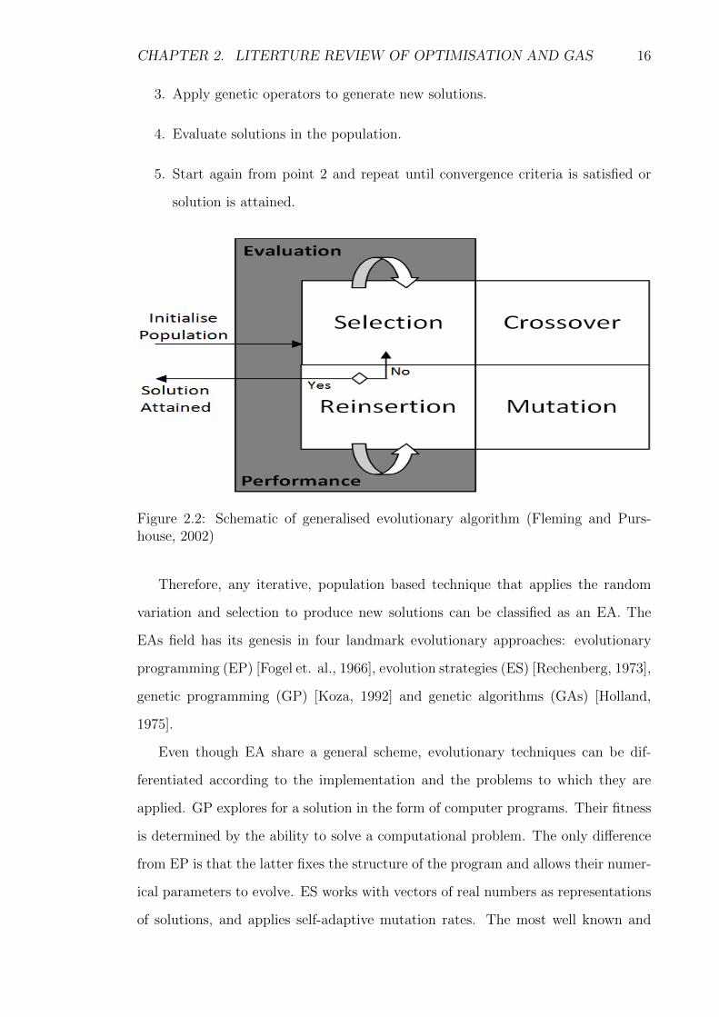
2.3.1 Evolutionary Algorithm

Evolutionary algorithms (EAs) are techniques that develop ideas of biological evolu-

tion for searching the solution of an optimisation problem, founded on the principles

of natural selection [Darwin, 1859] and population genetic [Fisher, 1930]. They re-

late to the principle of survival on a set of potential solutions to generate gradual

approximations to the optimum. A new set of approximations is created by the pro-

cess of selecting individuals according to their fitness and breeding them together

with operators stimulated from genetic processes. Figure 2.2 illustrates a schematic

of generalised EA techniques.

The main loop of EA includes the following steps:

1. Initialize and evaluate the initial population.

2. Perform competitive selection.


3. Apply genetic operators to generate new solutions.

4. Evaluate solutions in the population.

5. Start again from point 2 and repeat until convergence criteria is satisfied or

solution is attained.

Figure 2.2: Schematic of generalised evolutionary algorithm (Fleming and Purs-house, 2002)

Therefore, any iterative, population based technique that applies the random

variation and selection to produce new solutions can be classified as an EA. The

EAs field has its genesis in four landmark evolutionary approaches: evolutionary

programming (EP) [Fogel et. al., 1966], evolution strategies (ES) [Rechenberg, 1973],

genetic programming (GP) [Koza, 1992] and genetic algorithms (GAs) [Holland,

1975].

Even though EA share a general scheme, evolutionary techniques can be dif-

ferentiated according to the implementation and the problems to which they are

applied. GP explores for a solution in the form of computer programs. Their fitness

is determined by the ability to solve a computational problem. The only difference

from EP is that the latter fixes the structure of the program and allows their numer-

ical parameters to evolve. ES works with vectors of real numbers as representations

of solutions, and applies self-adaptive mutation rates. The most well known and


successful among evolutionary algorithms are genetic algorithms (GAs). They have

been explored by John Holland in 1975 and exhibit the necessary effectiveness.

Further, GAs were popularised by Goldberg (1989) and consequently, the ma-

jority of control applications are approved and implemented by this approach. GAs

are based on the fact that the role of mutation improves the individual quite seldom

and, therefore, they rely mostly on applying recombination operators.

2.4 Standard Genetic Algorithms

Standard genetic algorithms (SGAs) are a stochastic global search technique based

on the metaphor of natural biological evolution. This technique sustains a set of can-

didate solutions to a specified problem, which then evolve applying artificial genetic

operators such as selection, crossover and mutation. SGAs work by merging the Dar-

winian “survival of the fittest” principle with a probabilistic information exchange

approach encouraged by the processes of natural genetics, to form a structured yet

randomised search algorithm that assures to be well competent of identifying op-

timal, or near-optimal solutions, to a wide range of search, optimisation and machine

learning problems.

As discussed earlier, SGAs have been developed by John Holland, his colleagues,

and his students at the University of Michigan. Studies by Holland (1975), De Jong

(1975), Goldberg (1989), and others have demonstrated its superiority performance

of SGAs by theory and experimentation. More information on SGAs and a list of

practical applications can be found in Shopova and Vaklieva-Bancheva (2006) Fogel

(1994), Goldberg (1994), Randy and Sue (2004) and the introductory textbooks

by Goldberg (1989) and Mitchell (1996). Because of their exclusive structure and

function, SGAs diverge from more traditional and modern search procedures and

algorithms in some very fundamental ways, making them ideal candidates as global

function optimisers.

Recent studies illustrated the SGAs performed reasonably well compared to other

evolutionary algorithms (Wu and Ji, 2007) (Kachitvichyanukul, 2012) (Silberholz

and Golden, 2010) (Adewole et. al., 2012) (Bajeh and Abolarinwa, 2011) (Gamal


et. al., 2014) (Nagaraj and Murugananth, 2010).

Another attribute of SGAs that distinguishes them from most conventional and

modern search methods is that they work with a coding of the parameter set and

not with the parameters themselves. This gives them direct applicability to an

exceptionally wide range of non-numerical, discrete, combinatorial, and mixed op-

timisation problems. Kachitvichyanukul (2012) has suggested that SGAs are more

suitable for discrete PID optimisation than the PSO and DE, which are suitable for

continuous PID optimisation.

Most conventional and modern optimisers based on continuous parameter vari-

ations cannot normally be used for the solution of such problems. The influences of

SGAs come from the statement that they are robust and thus, have the prospect-

ive to apply and solve efficiently many difficult problems without constraints. As

expected, SGAs are not certain to locate the globally optimal solution to a specific

problem, but are generally excellent in locating reasonably fine solutions to a wide

range of problems which is rapidly acceptable.

Figure 2.3: Efficiency of different classes of search techniques across a problemcontinuum (Goldberg, 1989)

Figure 2.3 illustrates the better perception of the significance of robustness in

a search technique. According to the figure, the specialised technique is well per-


forming in the problem area it has been designed for, but its efficiency drops rapidly

when applied in different problem areas. On the contrary to that, entirely random-

ised techniques, such as random walk, are executing consistently in a wide range

of problem areas, but their efficiency is in general low. Robust techniques, such as

SGAs, unite efficiency with consistency and achieve a suitable performance across

a wide range of domains. Even though other specialised techniques are probably

perform better than SGAs for solving specific problems but the SGAs can provide

a very effective, efficient and fast solution.

2.4.1 Multi-Objective Optimisation by SGAs

Being a population-based approach, SGAs are well suited to solve multi-objective

optimization problems. A generic single-objective SGAs can be modified to locate

a multiple non-dominated solutions set in a single execution. The ability of SGAs

to simultaneously search different regions of a solution space makes it possible to

locate a diverse set of solutions for difficult problems with non-convex, discontinuous,

and multi-modal solutions spaces. In addition, most multi-objective SGAs do not

require the user to prioritize, scale, or weigh objectives. Therefore, SGAs have be

en the most popular heuristic approach to multi-objective design and optimization

problems.

The first multi-objective SGAs, called vector evaluated SGAs (or VEGA), was

proposed by Schaffer (1985). Afterwards, several multi-objective evolutionary al-

gorithms were developed including Multi-objective Genetic Algorithm (MOGA)

(Fonseca and Fleming, 1995). Since then many research works has been under-

taken to improve the MOGA (Fonseca and Fleming, 1998) (Jensen, 2003) (Xiujuan

and Zhongke, 2004). However, the MOGA is not considered here as a part of this

research work.

2.4.2 Premature Convergence

One of the most general phenomena that encountered in optimisation is premature

convergence in modern heuristic algorithm (Vanaret et. al, 2013). A process of


optimisation prematurely converged to a local optimum if the initial population is

generated randomly from poorly selected search space region [Ursem, 2003] [Vanaret

et. al., 2013] [Chaiwat and Prabhas, 2011]. In another term, if population is not se-

lected from optimal search region it becomes complicated to locate the elite solution

of the problem whether in the case of initial population selection or the selection of

population for the next generation. Figure 2.4 illustrates several common phenom-

ena (factors) to take into account when the initial population is generated randomly.

Figure 2.4: Phenomenon of initial population

The search space selection is one of the grounds that lead to premature con-

vergence. Well selected search space region will brought the elite group within the

feasible region to avoid premature convergence [Rajarathinam et. al., 2015]. In

fact, the well selected search space regions will sustain the population diversity.

Preservation of search space and population diversity is correlated with sustaining a

well balance between exploration and exploitation [Weise, 2009]. An exploration is

applied to examine new and unknown region in the search space, and exploitation

applies the previously visited and identified information to assist locate the elite

solution [Rajarathinam et. al., 2015].

A brief knowledge about variety methods of sustaining the population diversity

and selective pressure to avoid the premature convergence were proposed (Deepti

and Shabina, 2012). Nakisa et. al., (2014) presented a comprehensive survey of the

various PSO-based algorithms such that PSO is a computational search and optim-

ization method based on the social behaviours of birds flocking or fish schooling.


Chaiwat and Prabhas (2011) proposed the self-adaption technique to control the

population diversity without explicit parameter setting. The technique is based on

the competition of preference characteristic in mating. Based on simulation results,

the adaptive technique has potential to adapt the diversity of the population for a

given problem without the knowledge of correct parameter setting. Also, it has a

good performance in finding the solution.

A number of basic variations have been developed due to solve the premature

convergence problem and improve quality of solution founded by the PSO. Suri

et. al., (2013) proposed that Elitism technique was augmented within Genetic Al-

gorithm allowing the best solution from any generation to be carried across the new

population allowing it to sustain. Social Disaster Techniques (SDT) was used when

premature convergence occurred and the problem of premature convergence may be

avoided by creating random offspring and inserting diversity in the population (Ra-

madan, 2013). This paper attempted to use the both concepts of Elitism and Social

Disaster techniques spanning across various generations. A previous solution was

chosen and it has been looked upon how Elitism and Social Disaster techniques fares

towards the same problem. Malik and Wadhwa (2014) proposed a collaboration of

dynamic genetic clustering algorithm (SGCA) and elitist technique for preventing

premature convergence. This proposed technique provides a strong immunity to

mutation and crossover operators to be trapped in local optima.

Based on the complex Box technique, a boundary search method for optimisation

problems in the case of the optimal solution at the boundary was proposed (Zhu

et. al., 1984). It has been demonstrated and verified, if there is an optimal solution

at the boundary constraint set. Recently, a modified GAs is applied in solving the

n-Queens difficulty in chessboard (Heris and Oskoei, 2014). The holism and random

choices cause solving difficulties for SGAs in searching a large space. To improve

the solving difficulty, the minimal conflicts algorithm is collaborated with SGAs.

The minimal conflicts algorithm gives a partial view for SGAs by a locally searching

space. But, the collaboration of algorithms consumed time for searching.

An approach called the self-adaptive boundary search strategy for penalty factor


selection within SGAs was proposed (Wu and Simpson, 2002). This approach guides

the SGA to preserve around constraint boundaries and improves the efficiency of

attaining the optimal or near optimal solution. A technique for resolving the struc-

tural optimisation difficulties in quantising the subjective uncertainties of active

constraints is proposed by fuzzy logic formulation (Wu and Wang, 1992).

Another method to improve the prematurity and to sustain the diversity popu-

lation was proposed by Niche Genetic Algorithm (NGM) associated with isolation

mechanism (Lin et. al., 2000). A comparison study was done on NGM and Anneal-

ing Genetic Algorithm where the Annealing Genetic Algorithm has better premature

convergence (Tu and Mei, 2008). However, the Annealing Genetic Algorithm is time

consuming by extra procedures.

Another method, named Accelerating Genetic Algorithm (AGM) was proposed

to resizing the feasible region into the elite individual’s adjacent region for better

local searching and convergence (Jin et. al., 2001). Search space boundary re-

duction for the candidate diameter for each link by pipe index vector and critical

path method, along with modified genetic operator’s derivatives, was proposed (Ma-

hendra et. al., 2008) (Vairavamoorthy and Ali, 2005). Further, an improved AGM

based on the saddle distribution by which adding random individuals into the initial

population to increase the searching ability of optimal solution was proposed (Xu

et. al., 2012).

2.4.3 SGAs in Model Parameter Identification

The SGAs have been employed succesfully in the process model parameter identi-

fication of both linear and non-linear system’s models. Kampisios et. al., (2008)

applied off-line GAs in identification of linear induction motor electrical parameters

in function of flux levels based on experimental transient measurements from a vector

controlled induction motor (I.M.) drive. Liu et. al., (2014) demonstrated a para-

meter identification for the determination of hydraulic and water quality parameters

such as the longitudinal dispersion coefficient, the pollutant degradation coefficient,

velocity by coupling the GAs with finite difference method (FDM).

Wong et. al., (2011) applied the GAs to generalise and learn protein-DNA bind-


ing sequence representations. The generalized pairs are shown to be more meaningful

than the original transcription factors and transcription factor binding sites (TF-

TFBS) binding sequence pairs. The proposed method by GAs assists to extract

such many-to-many information from the one-to-one TF-TFBS binding sequence

pairs found in the previous study, providing further knowledge in understanding the

bindings between TFs and TFBSs.

Kiperwasser et. al., (2013) improved and proposed the dense pixel matching

using the GAs in rectifying the image scenario. An elegant approach is allowing,

optimising and matching fitness functions has recently shown a 20% of quality im-

provement while performing fast convergence. The effectiveness and efficiency of

GAs has been well demonstrated by Roeva (2008) and Benjmin et. al., (2008) for

model parameters identification of fed-batch cultivation processes. Further, Maria

et. al., (2011) applied SGAs and multi-population GAs for a parameter identification

of a yeast fed-batch cultivation of S, (cerevisiae).

Mathew et. al., (2014) successfully applied the GAs based a segmentation ap-

proach in identification of defects in glass bottles. The GAs has produced high

sensitivity, high specificity and high accuracy of 92%, 93% and 93% respectively.

The method produced effective results and hence this tool shall be useful for food

processing industries for the Quality Inspection of the glass bottles.

Aloysius et. al., (2012) successfully applied the GAs in order to maximize the

revenue of airline by optimizing the flight booking and transportation terminal

open/close decision system. Gondro and Kinghorn, (2007) aligned the multiple

sequence alignment which plays an important role in molecular sequence analysis.

An alignment is the arrangement of two (pair-wise alignment) or more (multiple

alignment) sequences of ’residues’ (nucleotides or amino acids) that maximizes the

similarities between them. Algorithmically, the problem consists of opening and

extending gaps in the sequences to maximize an objective function (measurement

of similarity). The GAs is well suited for problems of this nature since residues and

gaps are discrete units.

Further, the SGAs have been successfully applied in the field of medicine and


biology. Wang et. al., (2007) demonstrated an exploitation of different methods for

intergenic distance, cluster of orthologous groups (COG) gene functions, metabolic

pathway and microarray expression data. The GAs is applied for integrating the

four types of data of predicting operons in prokaryote. Nur et. al., (2012) proposed

and demonstrated GAs to estimate the parameter of warranty cost model with

warranty claim data collected from Malaysian automotive industry. Further, Scarf

and Majid, (2011) introduced the mixed exponential distribution with GAs since

zero delay time may occur in some defects. As a result, they found that the mixed

exponential models is better than ordinary exponential.

2.4.4 SGAs in Control Parameter Optimisation

Numerous GA-based techniques have been developed for the optimal control design

and control parameter optimisation. Altinten et. al., (2008) successfully applied the

GAs to optimise the PID parameters for temperature control of a jacketed batch

polymerization reactor and to track performance of optimal temperature profile.

Further, Altinten et. al., (2010) applied the GAs for self-tuning PID control for

the complex semi-batch polymerisation reactor processes. The change of monomer

concentration is causing a change in reaction rate varies nonlinearly over the time.

The simulation results assured that GAs control the temperature very well.

Slavov and Roeva, (2012) applied binary coded SGAs to optimise the discrete

PID parameters for sustaining the glucose concentration during the E. Coli fed-

batch cultivation process. Jan et. al., (2008) proposed and demonstrated robust

PID control scheme by SGAs for the permanent magnet synchronous motor is im-

plemented by a DSP-based fully discrete controller.

Kim et. al., (2008) proposed an improved GAs technique to tune an optimal

PID parameter to control the reverse osmosis (RO) plant with minimum overshoot

and fast settling time compared with conventional tuning techniques. Yin et. al.,

(2004) successfully applied GAs to tune PID parameter for low damping and slow

response process. Zain et. al., (2009) applied GAs for optimizing PID parameters

to control a single-link flexible manipulator in vertical motion. Simulation results


revealed that the optimum PID parameters by GAs enable the system to perform

well in reducing vibration at the end-point of the manipulator.

Nithyrani et. al., (2013) applied SGAs to tune an optimal discrete PID paramet-

ers for liquid tank process temperature. Simulation reveled that the binary coded

SGAs performed well to sustain the liquid temperature and compared with conven-

tional techniques. Zhang et. al., (2010) proposed a PID parameter optimization by

performance index based on integral of absolute error, rise time, controller output

and overshoot. Simulation results indicate that the GAs is a practical and effective

method in optimizing the control parameters.

Perez and Basterrechea, (2004) demonstrated an application of SGAs for pre-

dicting the far-field radiation of an antenna from synthetic near-field data. Simula-

tion results compared and revealed that the binary coded SGAs well performed for

large antennas as it applies small population size than real coded genetic algorithms

(RCGAs). Gauri and Kulkarni, (2013) well applied the binary coded SGAs to op-

timize the discrete PID parameters for missile altitude control system.

Valarmathi et. al., (2012) demonstrated an optimisation of PID parameters by

binary coded SGAs for a non-linear liquid conical tank system. Jayachitra and

Vinodha, (2014) well applied binary coded SGAs to optimise the discrete PID con-

trol for continuous stirred tank reactor (CSTR) process. The control performance

of CSTR process has enhanced by integrating weighting factor with combined con-

ventional objective functions. Patrascu et. al., (2011) applied the discrete PID

parameters which are optimised by SGAs for non-linear 3D crane multi-input multi-

output (MIMO) systems.

In recent years, the GAs is well applied in control strategy for robotics techno-

logy. Abo-Hammour et. al., (2011) demonstrated binary coded GAs based control

suitability for autonomous selection of a collision free path for the manipulator that

minimizes the deviation between the generated and the desired Cartesian path. The

control parameters are satisfies the joints limits of the manipulator, and maximize

the minimum distance between the manipulator links and the obstacles. Ghanbari

and Noorani, (2011) proposed a control technique for a new crawling gait to develop


in a modular robot by GAs. Wang et. al., (2012) proposed a new approach to

generate the original motion data for humanoid motion planning by binary coded

GAs.

The state generator is developed based on the GAs, which enables users to

generate various motion states without using any reference motion data. By spe-

cifying various types of constraints such as configuration constraints and contact

constraints, the state generator can generate stable states that satisfy the constraint

conditions for humanoid robots. Arturo et. al., (2013) proposed a technique of integ-

ration of gain-phase margin method with the binary coded GAs for discrete control

strategy of industrial robot and computer numerical control (CNC) machines. The

proposed technique is performed well as expected and compared with RCGAs and

conventional gain-phase margin method. Some other applications to multivariable

process control are reviewed in chapter 6.

2.4.5 An Application of SGAs for Furnace Type Processes

Literature survey revealed that not numerous research works has been undertaken

on an application of SGAs for the glass furnace or furnace type processes in model

parameters identification and control parameters optimisation.

Joao and Pedro, (2003) introduced an architecture for the operation system of

industrial recuperative-type glass furnace. The expert control is integrated with

GAs for control optimisation and solves the multi-objective optimisation problems,

respectively. Zarko et. al., (2010) presented an application of GAs with fuzzy control

for optimising PID parameters for fluidized bed combustion (FBC) chamber. The

results revealed that the closed-loop systems have a fast rise response with small

overshoot.

Srisertpol et. al., (2011) proposed an estimation method for the mathemat-

ical model using the open-loop identification for the slab reheating furnace walking

hearth type with GAs in heating curve up process. The responses of experimental

and simulation are consistent. Liu and Guo, (2013) presented the fuzzy neural net-

work temperature control system based on SGAs for resistance furnace which has


nonlinear characteristics with big inertia and great delay.

The artificial neural network structure and parameters are trained with fuzzy

control rules. The membership functions of fuzzy control rules are determined by

using the neural network’s self-learning and adaptive ability. The SGAs is adopted

to train the controller’s connecting weights. The simulated results indicate that

the fuzzy neural network temperature control system is more dynamic, robust, and

highly precise.

Ping et. al., (2014) presented and applied the dynamic matrix predictive control

based on GA to the electrode regulator systems of industrial arc furnace. The

optimal control law is obtained by rolling optimization. The simulation result shows

a significant improvement on the dynamic performance and the robustness of the

system.

2.5 Review of PID Control Strategies

The PID controllers have been at the heart of control engineering practices for the

last seventy-five years. The first tuning rule for setting up controller parameters

was defined by Callender (1935). The proposed technique comprises design of a

PD controller for a process which is exactly modelled by an integrator plus delay

time. After eight years of Callendar work, Zeigler-Nicholas proposed two classical

techniques for PI/PID control parameters identification. These techniques are still

extensively applied, either in novel structure or with some improvement. The first

technique was derived from an open-loop step response of the process, which is

characterised by two unknown parameters. The unknown parameters were estab-

lished from a unit step response of a process and applied to identify the controller

parameters (Zeigler-Nicholas, 1942).

The second technique of Zeigler-Nicholas (1943) was derived from frequency re-

sponse of a process. The parameters of P/PI/PID controller were determined from

gain margin, GM and phase crossover frequency, ωpc. Chien et. al., (1952) per-

sonalized the Zeigler-Nicholas step response technique by applying fastest response

without overshoot or with 20% overshoot as design criteria. The proposed technique


made a significant observation that tuning for set-point response or load disturb-

ance response should be different. Cohen and Coon (1953) designed a technique

which was derived from First-Order plus Dead-Time (FOPDT) model structure.

The proposed technique does suffer, nevertheless, from the decay ratio being too

small, which means that the closed-loop systems obtained have low damping and

high sensitivity.

In the beginning of twenty first century, the applications of PID parameters on

complex and higher order processes are well enhanced. Majhi and Atherton (2000)

developed a controller design technique on a modified smith predictor strategy, which

leads to significant improvements in its regulatory capacities for reference inputs and

disturbances. The first order or second order response of the plant model is assumed

and the controller parameters are approximated by applying precise analysis from

the peak amplitude and frequency of the process output obtained from a single relay

feedback test. The robustness of controller is noticeable from results obtained using

incorrect time delay values in the plant model.

Wang and Shao (2000) proposed a technique for PI controller based on load

disturbance rejection with constraint which is the Nyquist curve of the loop transfer

function is tangent to a line parallel to the imaginary axes in the left-half of the

complex plane. The method satisfies both robustness and performance requirements,

but is restricted to PI controller and does not provide an extension to the PID

controllers.

Wang et. al., (2001) developed internal model control-based (IMC) single-loop

controller design technique. The model reduction technique was applied to approx-

imate the best single loop controller for the IMC controller. This technique can be

automatic for on-line tuning. The technique gives an alternative to attain specified

closed-loop performance at the cost of controller complexity or retain simple PID

controller with possible deterioration in the closed-loop performance. So, this tech-

nique is not well applicable for higher order processes to get the desired closed-loop

response with PID controllers.

Skogestad (2003) developed an analytic rule for PID controller tuning which


is simple and still gives good closed-loop behaviour. The starting point has been

the IMC-PID tuning rules that have achieved widespread industrial acceptance.

The rule for integral term has been modified to improve disturbance rejection for

integrating processes. Furthermore, rather than deriving separate rules for each

transfer function model, there is a single tuning rule for FOPDT or Second-Order

plus Dead-Time (SOPDT) model. The only drawback of the method is that the

model order reduction is required for higher order systems.

The design of PI controllers to achieve desired frequency and time domain spe-

cifications simultaneously was proposed by Hamamci and Tan (2006). The per-

formance of frequency domain, GM and phase margin (PM), and the performance

of time domain, settling time and overshoot were defined prior to the design. To

meet the specified performance values, a method which presents a graphical relation

between the required performance values and the parameters of the PI controller

for a given model. The graphical relations are limited to the design of PI controller

and extension to the PID controller is not cleared.

An alternative PID auto-tuning approach had been proposed to the popular step

response and relay-based technique by Gyongy and Clarke (2006). The approach

involves injection of a variable-frequency probing signal into the closed-loop. The

technique differs from most existing methods in that the tuning was performed on-

line, which is whilst; the controller was undertaking closed-loop control. As a result,

it is providing single-shot auto-tuning while continuous adaptation of the control-

ler. In this approach, ease-of-use was ensured by a semi-automatic initialization

procedure only, which employs the results and knowledge of a prior step-test.

Bitschnau and Kozek (2009) applied a PID controller with feed-forward compens-

ation technique for continuous heat treatment steel strips type furnace. Simulation

result revealed that the PID with feed-forward compensation technique is able to

react to temperature parameter variation of the proposed material in reasonable

time. In model based design of PID controllers, Malwatkara et. al., (2009) pro-

posed for higher-order oscillatory systems. This method has no limitations regard-

ing systems order, load changes, time delays and oscillatory behaviour. Selection of


coefficients through the use of frequency responses with reduced model is achieved

based on third-order modelling. The tuning of the PID parameters is obtained from

a reduced higher-order model. This technique seems to be simple, effective, and

improved performance of the overall system.

Improved Electromagnetism-like (EM) algorithm with genetic algorithm (GA)

technique (IEMGA), for optimization of fractional-order PID (FOPID) controller is

proposed by Ching and Chang (2010). IEMGA is a population-based metaheuristic

algorithm originated from the electromagnetism theory. For FOPID control optim-

ization, IEMGA simulates the “attraction” and “repulsion” of charged particles by

considering each controller parameters as an electrical charge. The neighborhood

randomly local search of EM algorithm is improved by using GA and the competitive

concept. IEMGA has the advantages of EM and GA in reducing the computation

complexity of EM. This method gives effective performance.

A novel fractional order (FO) fuzzy-PID controller has been proposed by Saptar-

shi et al. (2011), which works on the closed loop error and its fractional derivative

as the input and has a fractional integrator in its output. The fractional order

differ-integrations in the proposed fuzzy logic controller (FLC) are kept as design

variables along with the input–output scaling factors (SF) and are optimized with

genetic algorithm (GA). The closed loop performances and controller efforts in each

case are compared with conventional PID, fuzzy PID and PI Dm controller subjected

to different integral performance indices. Simulation results show that the proposed

fractional order fuzzy PID controller out performs the others in most cases.

In the literature review of Hitay et. al., (2012) a classical proper PID controllers

are designed for linear time invariant plants whose transfer functions are rational

functions of sa, where 0 < a < 1, and s is the laplace transform variable. Effect of

input–output time delay on the range of allowable controller parameters is invest-

igated. The allowable PID controller parameters are determined from a small gain

type of argument for finite dimensional plants.

There are many online automatic PID parameters tuning methods have been

proposed to improve the control performances, Nevertheless, satisfactory control


performances are not able to attain by above mentioned methods due to inapplicab-

ility of wide operating region of the controller. Also, a high mathematical approach

is complicating the implementation to industrial process.

Heuristic optimization is a technique of locating good solutions at a reasonable

computational cost without being able to guarantee either feasibility or optimal-

ity, or even in many cases to state how close to optimality a particular feasible

solution is (Reeves, 1995). By means of superiority for global optimisation and bet-

ter robustness, the SGA is applied here to enhance the capabilities of conventional

PID tuning techniques in online identification without complicated mathematics.

Recently, SGAs has been extensively studied by many researchers in searching for

optimal PID parameters due to its high potential of escaping being trapped a local

minimum as discussed in detail at chapter 2.

2.6 Review of Multivariable PID Tuning Strategies

For a complex multivariable process, a decentralised control strategy is generally

applied, and has always been in the attention of many researchers, for developing

a precise control strategy to enhance the performance of multivariable processes.

However, difficulties are encountered in designing the decentralised control due to

the loop interactions.

A literature survey reveals that there are several classified tuning methods sug-

gested to tune decentralised controllers for multivariable processes such as detuning

(Monica et. al., 1998), sequential design (Hovd and Skogestad, 1994) and independ-

ent design (Lee et. al., 2001) methods.

In the detuning method, the individual controllers of the multi-loop control sys-

tem are first designed without considering the interactions between control loops,

and then, all settings are detuned taking into account the interactions until some

stability criterions are satisfied. A well-known method of this type is the biggest log

modulus tuning (BLT) method (Luyben W. L., 1986).

Initially, the single-input, single-output (SISO) controllers are obtained by using

the Ziegler-Nichols settings. Detuning is then performed by adjusting one parameter


F , where F is determined via a Nyquist-like plot of the closed-loop characteristic

polynomial. Since the biggest log-modulus, which measures how far the control

system is from being unstable, is obtained equal to 2N (N is the order of system) by

adjusting F , the controller parameters for multi-loop control systems are determined.

In the sequential design method, each controller is designed sequentially with the

previously designed controllers implemented. Basically, a controller is first designed

by considering the selection of an input-output pair and this loop is closed. A second

controller is designed by considering the second input-output pairing since the first

loop closed and so on. The sequential design method can be used for complex

interactive problems where the independent design method does not work. A po-

tential disadvantage of this design method is that failure tolerance is not guaranteed

when the previous loops fail. When the system outputs can be decoupled in time,

the sequential design method can be effectively used for the design of multi-loop

controllers.

In the independent design method, each controller is designed based on the cor-

responding diagonal element of the multivariable process transfer function model,

while the off-diagonal interactions should be taken into account by considering some

inequality constraints on the process interactions. The main advantage of independ-

ent design is that the failure tolerance is guaranteed automatically. However, it is

conservative due to the assumptions of the design method. This design method is

effective when the system is diagonally dominant.

In general, these tuning methods have achieved a certain degree of success in

the design approach. However, these tuning methods do exhibit weaknesses and can

suffer in compensating the couplings between loop interactions of a multivariable

system. To improve the compensation of loop interactions, the effective open-loop

(EOP) method was introduced (Huang et. al., 2003). The EOP method considers

all other loop interactions while adapting the i − th control parameters for the

i − th EOP. But, the EOP method produces model approximation error due to

mathematical complications as the model dimensions are increased. Thus, the EOP

method is mainly applicable for low dimension models.


Another successful approach is that of relay auto-tuning, which is a combination

of single loop relay auto-tuning and the sequential tuning method (Loh et. al.,

1993). This method appears to perform well, but a multivariable system with large

multiple dead times exhibits poor performance.

In recent years, to improve the entire control performance and robust stability,

systematic approaches based on the generalised IMC-PID design method (Grosdidier

and Morari, 1987) and the reduced effective transfer function (RETF) by inverse

response behaviour method (Truong et. al., 2009) have been introduced for mul-

tivariable processes. But, both methods involve a complex mathematical approach

to design the decentralised controllers. In general, a question always arises about the

wellness of control optimisation and the flexibility due to the application constraints

by these design methods.

In decentralized control of 2Ö2 MIMO systems, the control system consists of

two such controllers. Each of them takes care of a single loop only and the inter-

action between the two loops is greatly reduced, unlike the centralized PID control

where a similar 2Ö2 controller structure is assumed to stabilize a two-input two-

output (TITO) process (Tavakoli et. al., 2006) (Fernando et. al., 2008). However,

the decentralized controller design can be easily applied if the loops do not heavily

interact with each other, i.e. the corresponding Relative Gain Array (RGA) should

have a dominating principal diagonal. If the loop interaction changes the process

gains of the individual loops considerably, then well-tuned controllers for the indi-

vidual loops fail to keep the controlled variables at their respective set-points. In

such cases, pairing of any manipulated variable with any controlled variable results

in poor controller performance.

Applications of evolutionary algorithms have become very prominent to improve

the decentralised control for multivariable processes. Iruthayarajan and Baskar

(2009) and Wei (2007) used evolutionary algorithms and multi-crossover genetic

algorithms to minimize the summed integrated absolute error (IAE) for each loop

while tuning the PID controller parameters. Ramin et. al., (2008) designed a de-

centralized PID controller by minimizing total IAE for all loops using the colonial


competitive algorithm. Kai et. al., (2008) tuned PID controllers based on a closed

loop particle swarm optimizer (PSO) algorithm. Zhao et. al., (2012) minimized

integral square error (ISE) employing “two-lbests” based PSO for designing robust

PID controller for MIMO systems.

Vijula and Devarajan (2014) proposed the model reference adaptive control

(MRAC) technique for a multivariable quadruple tank process. The linearized model

of the quadruple tank system has a multivariable transmission zero and it is much

more difficult to control the system in non minimum phase condition than minimum

phase condition. The proposed controller can adjust the controller parameters in

response to changes in plant uncertainties and disturbances based on the specified

reference model and prevent the system from interaction between process variables.

It is shown by the simulation results that MRAC technique solves the dynamic prob-

lem of the quadruple tank process and it is convenient for controller design under

the requirement of the system.

A promising decentralised controller by SGAs was proposed for a multivariable

process (Vlachos et. al., 1999). The controller performance was defined by closed-

loop response in terms of time-domain bounds for both reference following and loop

interactions. An integrity theorem with SGAs to enhance the closed-loop system

stability when certain loops are failing or breaking down was proposed by Li et.

al., (2007). Recently, improved convergence of genetic algorithms was achieved by

introducing the multi-objective evolutionary algorithm (MOEA) which combines

two fitness assignments methods; global rank and dominance rank (Rani et. al.,

2012).

2.7 Why SGAs?

As discussed in section 2.4, the SGAs are selected for its united efficiency with

consistency, robustness and an ability of achieving a suitable performance across a

wide range of domains. As a result, in cases where other expert techniques exist

for solving specific problems and possibly perform better than SGAs, but SGAs can

provide a very effective and efficient solution. Further, the literature survey reveals


that the SGAs are not well applied and explored for glass furnace process neither in

model identification and control parameter optimisation.

On the subject of SGAs coding selection, the real-coded may have outperformed

the binary-coded in several cases. However, the literature reveals that the binary-

coded is predominantly applied for discrete control parameter identification for its

suitability and flexibility than the real-coded. In particular, exceptionally complex

processes such as robotics for humanoid motion and missile trajectory for defence

system. Therefore, the SGAs associate with binary-coded is selected for model

parameters identification and control parameter optimisation as the discrete PID

control will be designed for research.

2.8 Chapter Summery

In this chapter, an overview of optimisation algorithms as applied to the solution

of control engineering problems was discussed, followed by a brief introduction to

standard genetic algorithms (SGAs) as global function optimisers, with emphasis on

their fundamental differences and advantages over conventional search algorithms.

The most attribute of SGAs that distinguishes them from conventional and modern

search methods is that they work with a coding of the parameter set and not with the

parameters themselves. This gives SGAs direct applicability to an exceptionally wide

range of non-numerical, discrete, combinatorial, and mixed optimisation problems.

A literature survey was then presented, indicating a successful applicability of

SGAs in process model parameters identification and control parameters optimisa-

tion problems. On the subject of SGAs coding selection, the binary-coded SGAs is

selected as it is predominantly applied for discrete control parameter identification

in exceptionally complex processes such as robotics for humanoid motion and missile

trajectory for defence system for its suitability and flexibility than the real-coded.

Further, other applications of SGAs for glass furnace and furnace type processes

were outlined. Finally, a successful tuning strategies in single-input single-out and

multi-variable PID are reviewed.

Chapter 3

Glass Furnace Modelling

Validation

3.1 Introduction

This chapter begins with a brief literature review of designing the combustion cham-

ber, which is fundamental to the developed methods for the glass furnace models.

Computational fluid dynamics method derived from radiative heat transfer were ap-

plied here to analyse the temperature distribution within the combustion chamber,

which is divided into finite zones.

Linearised energy balance equation in steady-state is improving the prediction

and accuracy of temperature distribution within finite zones. An assessment on

selected glass furnace model, which is designed by zones method is, provides a

deeper insight of model understanding and performance quantitative.

3.2 Review of Combustion Chamber

Literally, two main modelling techniques are strongly involved in furnace modelling

research; 1 – Empirical modelling techniques (Data-based) and, 2 – First-principles-

based modelling utilizing computational fluid dynamics (CFD) techniques. Empir-

ical Modeling Technique (Data-based) is a common and general approach that was

successfully applied in the glass industry and they result in fast models (Muller et.

36

CHAPTER 3. GLASS FURNACE MODELLING VALIDATION 37

al., 2003). This technique is able to learn and simulate the process behaviour just

from data, no further description is necessary. Parameters of these models have to

be determined from data measured on a real process.

There are some prominent empirical identification methods to determine the

model from measured data, such as Genetic Algorithm, AR, ARX, ARMAX, etc

(Ljung, 1999). A mathematical model using open-loop identification for the slab

reheating furnace by genetic algorithm was developed (Srisertpol et. al., 2011). The

responses of experimental and simulation systems were consistent. The approximate

mathematical model can be used to design an open-close burner to control the

suitable temperature with heating curve up and save energy of the slab reheating

furnace.

Another method of model identification of a process is performed by a learning

system, based on a fuzzy learning-by-examples algorithm (Joao and Pedro, 2003).

Process optimisation is carried out by an expert controller, and uses genetic al-

gorithms to solve a multi objective optimisation problem. Results of real and sim-

ulated experiments with the glass manufacturing process are blended with artificial

data. Even though the empirical modelling technique results a fast model for real

time simulation, difficulties arise in model identification due to long and painful tests

operation and the models are only valid for particular operating points. Moreover,

no glass companies are willing or allowing to perform the model identification tests

while the production is scheduled.

On the other hand, Computational fluid dynamics (CFD) solvers based on first-

principles are well established tools in the glass industry and highly prominent for

thermodynamics. Depending on the fineness of the used grid for discretization of

the partial differential equations describing the process, the model of, e.g., a melter,

is typically described by tens of thousands equations. Hence, computation takes a

long time and simulators run only at a speed comparable to a real time. Also, a

lot of parameters, initial and boundary conditions have to be specified prior to the

simulation. Mostly for speed reasons the full-order CFD models are inappropriate

for real time design purposes.


A Proper Orthogonal Decomposition (POD) method is proposed for the collec-

tion of measurements of physical quantities (such as temperature) in position and

time (signals) to reduce the complexity of CFD models (Astrid, 2004). Following

ideas from Fourier series expansions, signals are represented as series of orthonormal

functions. These so-called basis functions approximate the spatial distribution of

the signal while the coefficients of the basis functions represent the time-varying

dynamics. A similar POD technique was applied to a CFD model of a glass feeder

(Astrid and Weiland, 2005). The original CFD model of a feeder described by 3800

differential equations was reduced to a non-linear model only with 18 equations, res-

ulting in significantly increased simulation speed. Turbulent combustion models for

fine CFD are extensively developed (Veynante, 2002). The model represents how

the turbulence influences the combustion. In particular, the Eddy-Break-Up and

the mixture fraction approaches are implemented in glass furnaces models.

Another simplified CFD and thermodynamic modelling approach by using POD

was proposed, which can be used to simulate glass melt temperatures, velocities

and chemical composition as a function of time and position from a given furnace

geometry, composition of raw materials, refractory properties and (time varying)

boundary conditions (Huisman, 2005). These models are able to calculate the time

dependent behaviour of the temperature profile more than 10000 times faster than

the initial CFD model.

Regardless of how accurately the CFD model reduction method is applied, there

is still a need for calibration of the CFD model so that it sufficiently simulates the

real furnace (Muller et. al., 2005). With the validated model they use black-box

identification to obtain suitable linear models for controller design. Research in

the CFD field is still going on model reduction, but accuracy of such a model is

dependent on the accuracy of the original CFD model.

3.3 Combustion Chamber Modelling Approach

The initial classical CFD approach, where conservation laws on energy, momentum,

mass and mass fraction constitute the backbone of the model is applied in model-


ling a combustion chamber (Ungan, 1996). The model consists of tens of thousands

equations for the combustion chamber. Today, with growth of computer processing

power combined with simplified CFD models, the combustion chamber model op-

erates at a very fine scale (Auchet, 2005). However, the computation time is high

and inadequate for real time. The structure of combustion chamber models follows

the different physical phenomenon in terms of characteristics, which are combustion

space, bath and walls (Carvahlo et. al., 1997).

In a combustion chamber, a radiative heat transfer is a common occurrence

and predominant. Therefore, identification of the combustion chamber geometry is

playing a great importance task to describe the decomposition of a chamber into

zones having uniform temperature and radiative properties (either gas volumes,

molten glass surfaces or refractory wall surfaces) (Auchet et. al., 2008).

The most common radiative heat transfer method for analysing the temperat-

ure and heat flux is Hottel zone method (Hottel and Cohen, 1958). This method

was used to analyse the radiation heat transfer in an enclosure containing gray

gas. Later, the zone method was applied and developed for more complex geomet-

ries (Hottel and Sarofim, 1967). Since then, the zone method is widely applied

by researchers to identify the combustion chamber due to low computational time

and great model accuracy. Therefore, the developed combustion chamber by zone

method is presented here.

The zone method was employed for predicting heat flux on the side walls of

enclosures and temperature distribution within the combustion chamber. In this

method, the whole space of the combustion chamber is split into zones and the

enclosure’s walls are divided into some finite surface parts (zones). By writing

energy balance equations for all surface and volume zones in steady state, a system

of linear equations are derived for the temperature fields on volume and surface

zones.

3.3.1 Radiative Heat Transfer between Zones

The heat transfer between a pair of zones is known as directed heat flux area coeffi-

cients. The amount of heat transfer between surface to surface (SS), gas to surface


(GS) and gas to gas (GG) in a combustion chamber can written as,

QiS ,jS =→

SiSjEi −←

SiSjEj (3.1)

QiG,jS =→

GiSjEg,i −←

GiSjEj (3.2)

QiG,jG =→

GiGjEg,i −←

GiSjEg,j (3.3)

where→SiSj and

←SiSj are heat flux area between surface zone i and surface zone j,

Eg,i is black emissive power of gas and Ej is black emissive power of surface. The

radiative emissive power of each zone depends on temperature (Ei = σT 4; where σ

is the Stephan-Boltzman constant).

Apart from directed flux area, there are two more important coefficients in radi-

ation calculation that are applied in zone method; total exchange area and directed

exchange area. Table 3.1 illustrates the coefficients of radiation and respective ef-

fective parameters.

Table 3.1: Radiation Coefficients of Zone MethodCoefficients Symbols Effective Parameters

Directed FluxArea

→SiSj,

→GiSj,

→GiGj

Enclosure’s geometry, Absorptioncoefficient of gray gas, Surface emissivity

coefficient, Temperature of radiation source.Directed

Exchange Areasisj, gisj, gigj

Enclosure’s geometry, Absorptioncoefficient of gray gas.

Total ExchangeArea

SiSj, GiSj, GiGjEnclosure’s geometry, Absorption coefficientof gray gas, Surface emissivity coefficient.

The directed exchange area coefficient is also known as photometric coefficient

and this coefficient quantifies how the elements radiate each other, and is only

depending on the geometry and the photometric coefficients of the gas and the

different surfaces filling the chamber. In the present model, all elements are assumed

grey, i.e. with directed exchange area coefficients not depending on the wavelength.

This means that the heat transfer computations can be done globally on the whole

spectrum.


Directed exchange areas are kind of visibility factors, and following expressions

shows the case of visibility factor between,

A surface element Ai and a surface element Aj,

sisj =

ˆ

Ai

ˆ

Aj

cos θi cos θj exp (−krij)πr2ij

dAidAj (3.4)

A gas element Vi and a surface element Aj,

gisj =

ˆ

Vi

ˆ

Aj

k cos θj exp (−krij)πr2ij

dVidAj (3.5)

A gas element Vi and a gas element Vj,

gigj =

ˆ

Vi

ˆ

Vj

k2 exp (−krij)πr2ij

dVidVj (3.6)

where, rij is the size of the vector that connects the centres of two elements to each

other, θi and θj are the angle between the normal vector of surface elements and

aforementioned vector, and k is emissivity coefficient of gas.

So far, the total exchange area been calculated by gray gas assumption from

combustion product. But, the gray gas is not the main product of combustion.

Thus, using gray gas assumption caused an unrealistic real gas model. Therefore,

the weight summation of gray gases method is applied. In this method, the following

expression is considered for emissive coefficient of real gas:

εg =n

Σi=0

ag,i(1− exp(kiPL)) (3.7)

where k, P and L represents the emissivity, partial pressure and effective path length

of the gray gases, respectively. Term i = 0 is related to limpid gas.

By using and considering this method, the water vapour and carbon dioxide

(CO2)and a limpid gas as the main products of combustion the coefficients of ag,i

have been calculated for several states of partial pressures (Viskanta and Mengue,

1987).


These coefficients are employed for calculating directed flux area from total ex-

change area by the following expressions, for

Surface-Surface zones:

→SiSj =

N

Σn=1

as,n(Ti)[SiSj

]k=kn

;←SiSj =

N

Σn=1

as,n(Tj)[SiSj

]k=kn

(3.8)

Surface-Gas zones:

→GiSj =

N

Σn=1

ag,n(Tg,i)[GiSj

]k=kn

;←

GiSj =N

Σn=1

as,n(Tj)[GiSj

]k=kn

(3.9)

Gas-Gas zones;

→GiGj =

N

Σn=1

ag,n(Tg,i)[GiGj

]k=kn

;←

GiGj=N

Σn=1

ag,n(Tg,j)[GiSj

]k=kn

; (3.10)

3.3.2 Energy Balance Equation

The first law gives a quantitative relation of energy balance equation by the variation

with time, t, of the heat generated in the sample, Q, due to the absorption of light

of incident power Pi, is given by

∂Q/∂t = Pi − q (3.11)

where, q is the power losses by radiation, convection and conduction.

For research, radiation is the only mechanism taken into account for energy

balance formulation due to its predomination. Thus, the parameter q should be

some function of the temperatures, T1 and T2, of both the regions involved. It

is denoted as the heat flux. In general, the dependence of the heat flux on the

temperature is non-linear.

The continuous energy interchange between separated bodies by means of elec-

tromagnetic waves, the net rate of heat flow, qrad, radiated by a body surrounded

by a medium at a temperature T1 is given by the Stefan-Boltzmann Law,


qrad = εσA(T 42 − T 4

1

)(3.12)

where A is the surface area of the radiating object and ε is the total emissivity of

its surface having absolute temperature T2.

To compute the rise of temperature, ∆T , of the back sample’s surface, the heat

term of equation 3.1 must be expressed as a function of that increase. It is given by

the relationship,

Q = ρcV∆T (3.13)

where ρ is the density, c is the specific heat and V = AL is the sample’s volume.

Differentiation of equation 3.13 with respect to time and substitution into equa-

tion 3.11 leads to:

∂∆T

∂t+

q

ρcV− PiρcV

= 0 (3.14)

where qrad is specified as radiation terms given by equation 3.12.

As described by non-linear relationships, the rates of radiative heat flow are de-

pendence on the temperature. This non-linearity makes complicated the analytical

solution of the energy conservation law as given by equation 3.14. A glimpse at

equation 3.12 shows that if the temperature difference ∆T = T2 − T1 is small, then

one could expand it as a Taylor series around T1 obtaining a linear relationship:

q = 4εσAT 31 (T2 − T1) = hA∆T (3.15)

The h = 4εσT 31 can be considered as a radiation heat transfer coefficient. This

linearised energy balance equation is accurate above 1300K (Holladay, 2005).

3.4 Simulated Combustion Chamber Model

The combustion chamber that is identified and applied for further research here is

modelled from Fenton Art Glass Company, USA (Morris, 2007). This is an extended


research work of Holladay (2005) and was applied to develop a state space model

of an end-fired furnace in which the furnace was divided longitudinally into two

zones. The Zone 1 contains the burner flame “cylinder”, while Zone 2 is beyond the

end of the flame cylinder. Separate states are identified for the temperatures of the

refractory in the crown, the walls above the glass melt, the walls adjacent to the

two primary melt zones, and the floor of the furnace.

The furnace ends are also divided into similar zones constituting discrete states.

The glass melt itself contains a thin, surface layer and two thicker layers of strati-

fication. In all, 24 state variables are included in the model. The inputs are the net

thermal power provided by the flame and the ambient temperature.

Figure 3.1: 3D Furnace Combustion and Zone Divisions (Morris, 2007)

Simulations were performed in Simulink and Matlab and the results were verified

with real furnace from Fenton Art Glass Company. As illustrated in figure 3.1, the

dimensions of the furnace were approximated as 1.83m × 1.83m × 0.915m (6ft ×

6ft× 3ft).

The chamber is divided into two main zones; non-flame and flame zone. The

gas zone (α) consists of with and without flame. This division is kept steady as the

furnace is further divided throughout the depth of the glass. The glass surface (β)

is half inch thickness. This small thickness allows the assumption of no lateral heat

transfer. The final volume is the top half of the glass volume (χ) and the bottom of


the glass in the chamber (δ). The temperature within each volume of glass and gas

is assumed uniform.

Consequently, the heat transfer equation is simpler and gives fewer temperature

states within the furnace. However different volumes have different temperatures,

which allows for variations in temperature along the length and height of the furnace.

Refractory volumes consist of only the inner high temperature layer. A furnace is

constructed using two layers of refractory. The inner layer is an extreme temperature

refractory that is designed to resist the corrosion of the glass. The outer layer consists

of a lighter and insulating refractory.

The top half of the glass volume of non-flame zone temperature (Tgx2) is pre-

ferred as a final product output and feedback to controller to sustain the glass

temperature. The linearised energy balance equation 3.15 is applied and modified

with related variables for each gas and surface zones to identify 24 state-space vari-

ables corresponding to temperatures as listed in table 3.2. For example, the energy

balance equation of combustion zone α1 can be written as,

Qaα1 = Caα1dTaα1dt

(3.16)

Caα1dTaα1dt

=Qbwα1 +Qcα1 +Qswα1 +Qaα2 +Qgβ1+

Qgβ2 +Qgx1 +Qgχ2 +Qgδ1 +Qgδ2 +QFuel

(3.17)

Caα1dTaα1dt

= Abwα1Rbwα1

(Taα1 − Tbwα1) + Acα1Rcα1

(Taα1 − Tcα1)

+Aswα1Rswα1

(Taα1 − Tswα1) + Aaα2Raα2

(Taα1 − Taα2)

+OFβAgβ1Rgβ1

(Taα1 − Tgβ1) +(SF )OFβAgβ2

Rgβ2(Taα1 − Tgβ2)

+OFχAgχ1Rgχ1

(Taα1 − Tgχ1) + (SF )OFχAgχ2Rgχ2

(Taα1 − Tgχ2)

+OFχAgχ1Rgχ1

(Taα1 − Tgχ1) + (SF )OFδAgδ2Rgδ2

(Taα1 − Tgδ2) +QFuel

After expansion and rearrangement the heat transfer equation for the combustion

gases in α1 is,

dTaα1dt

= 1Caα1

[Abwα1Rbwα1

+ Acα1Rcα1

+ Aswα1Rswα1

+ Aaα2Raα2

+OFβAgβ1Rgβ1

+(SF )OFβAgβ2

Rgβ2+ OFχAgχ1

Rgχ1

+ (SF )OFχAgχ2Rgχ2

+ OFδAgδ1Rgδ1

+ (SF )OFδAgδ2Rgδ2

]+ Taα1 + Abwα1

(Caα1)Rbwα1Tbwα1

+ Acα1(Caα1)Rcα1

Tcα1 + Aswα1(Caα1)Rswα1

Tswα1 + Aaα2(Caα1)Raα2

Taα2


+OFβAgβ1

(Caα1)Rgβ1Tgβ1 +

(SF )OFβAgβ2(Caα1)Rgβ2

Tgβ2 + OFχAgχ1(Caα1)Rgχ1

Tgχ1

+ (SF )OFχAgχ2(Caα1)Rgχ2

Tgχ2 + OFδAgδ1(Caα1)Rgδ1

Tgδ1 + (SF )OFδAgδ2(Caα1)Rgδ2

Tgδ2 + QFuelCaα1

where, OF is the absorption factor based on capacity, SF is the shape factor relating

to radiation heat transfer, Caα1 is the capacitance of combustion gas in α1.

The other 23 state-space variables are listed in appendix.

Table 3.2: 24 State-space Variables of the Simulated Furnace ModelOrder State Variables Order State Variables Order State Variables

1 Taα1 9 Tgβ1 17 Tgδ12 Tbwα1 10 Tgβ2 18 Tbwδ13 Tcα1 11 Tgχ1 19 Tswδ14 Tswα1 12 Tbwχ1 20 Tflδ15 Taα2 13 Tswχ1 21 Tgδ26 Tcα2 14 Tgχ2 22 Tswδ27 Tswα2 15 Tswχ2 23 Tfwδ28 Tfwα2 16 Tfwχ2 24 Tflδ2

3.4.1 Brief Introduction of Glass Furnace

Figure 3.2 illustrates the block diagram of multivariable glass furnace which consists

of 24 states-space furnace model with feedback-loop and open-loop EO2 model. f1

and f2 is algebraic expression, f1 includes controller output and saturation, f2 is

thermal or energy demand (ED) includes specific heat (Cp) and low fuel calorific

heat value (LHV ) for determining the combustion energy, TSET is primary temper-

ature setting, Cg is glass control, AFR is air-fuel ratio, Tamb is ambient temperature,

·m is fuel flow in mass, QFuel is pressurised fuel based on ED for combustion, Tg is

glass temperature and EO2 is excess oxygen.

The glass temperature of the furnace is designed and controlled by primary input

vectors,·m (based on TSET with feedback error and AFR) and a secondary input

vector, Tamb. Any variation within these input variables could affect the Tg. The

EO2 is part of product element of methane combustion. The input vector of EO2

model is based on the AFR in mass (kg). The EO2 are developed based on the real

data collected from the Quinn Glass Limited, Chester by empirical technique for

1000sec with 5sec sampling interval (discussed in detail in section 4.5). The data


was gathered by the step input of increasing air ratio from 9.5 to 10.5 in volumetric

(ft3).

Figure 3.2: Block Diagram of Multivriable Glass Furnace

3.4.2 Validation of Combustion Chamber Model

The physical properties of the combustion chamber model were studied and the

main findings are as follows;

� The numerical coefficients of 24 state-space variables given in Morris (2007),

are unstable as an eigenvalue is located at right-side on s-plane (+45.3) as

shown in figure 3.3. Further close observation was carried out for each element

of the state matrix and it was found that 4 elements (Tgχ1, Tgχ2, Tgδ1, Tgδ2)

were absent (zero) for the non-flame forward wall temperature state-space

variable (Tfwα2).

� Another, state matrix element Tgχ2 was mistakenly identified as Tgχ1 and dis-

placed for the non-flame glass surface temperature state-space variable (Tgβ2).

Those missing and mistakenly identified elements were recalculated and the

24 state-space matrices updated. Cross reference was done with the updated


24 state-space variables simulation results and real data. Figure 3.4 shows the

corrected combustion model is now stable as expected as all the eigenvalues

are located at left-side on s-plane.

Pole-Zero Map

Real Axis

Ima

g A

xis

-80 -60 -40 -20 0 20 40-1

-0.8

-0.6

-0.4

-0.2

0

0.2

0.4

0.6

0.8

1

80 70 60 50 40 30 20 10

1

1

1

1 1 1 0.999 0.996

1

1

1

1 1 1 0.999 0.996

System: sys Pole: 45.3

Damping: -1 Overshoot (%): Inf

Frequency (rad/sec): 45.3

Figure 3.3: Eigenvalues of 24 Original State-Space Variables (Unstable)

Pole-Zero Map

Real Axis

Ima

g A

xis

-90 -80 -70 -60 -50 -40 -30 -20 -10 0-1

-0.8

-0.6

-0.4

-0.2

0

0.2

0.4

0.6

0.8

1

90 80 70 60 50 40 30 20 10

1

1

1 1 1 0.999 0.998 0.992

1

1

1 1 1 0.999 0.998 0.992

Figure 3.4: Eigenvalues of Corrected 24 State-Space Variables (Stable)

� All the stable 24 eigenvalues are identified. An eigenvalue located at -86.4,

another eigenvalue located at -2.87 and the rest of the eigenvalues are located

between −5.06× 10−6 to −3.47× 10−3. No complex poles. The eigenvalue at


-86.7 which is temperature of flame combustion gas zone (Taα1) is dynamic

and has fastest response. Then is followed by the eigenvalue at -2.87, which

is temperature of non-flame combustion gas zone (Taα2). The rest of the 22

eigenvalues are between −0.5× 10−5 to −3.5× 10−3.

� The glass furnace model was simulated on a computer using the simulation

package MatLab/Simulink. The time taken to complete a simulation tended

to be slowed and stopped when applying the default simulink solver options

(ode45 or ode23; standard variable step integration algorithms) as the simula-

tion model exhibits a stiffness problem. This is evident in the large variation

of the system eigenvalues, as discussed for figure 3.4 above. The ode23t (mod-

erately stiff/Trapezoidal) algorithm was therefore applied and was observed to

improve the simulation period and accuracy. The variable step was applied in

the simulation parameters as it is more robust than fixed step for stiff problems

(MathWorks, 2015).

� Open-loop step response of 24 state-space matrix combustion model has 54hrs

(2days and 6hrs) of 5% settling time for the glass temperature. According

to Morris (2007), the closed-loop response has 7.5hrs. Further simulation

testing carried out found that the controller gain used was excessive. With

excessive controller gain, the temperature of flame combustion gas zone (Taα1)

has high overshoot (1750K). Thus, these cause the refratories of chamber

(crown and walls) to have fast rise time and settling time in temperature less

than 1hr. A sudden, rise in temperature could cause a lessening in the life

time of chamber refratories (Carniglia, 1992). Appropriate controller tuning

is required to enhance the life time of refratories while making a concession on

the settling time of system response.

� A difficulty arose in understanding the input-output bounds to the glass fur-

nace process. The main fuel controller section has two sub-sections to determ-

ine QFuel for combustion. As shown in figure 3.5, the first section is the total


ED section (f2), which is estimated by thermal parameters such as LHV ,

AFR, Cp and TSET , gives ED(f2) =(

LHVCp×AFR + Tamb

)− TSET . The TSET

is set by operator, manually according to the daily throughput. The second

section is the fuel control section to control the·m according to the temper-

ature feedback error. Further, the·m is integrated with AFR and Cp, gives

f1 = Cp ×[(·m× AFR

)+·m]. The TFuel is total fuel consumption for total

period of simulation, gives TFuel =´ t0

·m(t)dt. As per thermal demand neces-

sity, the control should change when reset the TSET to attain the steady-state

temperature. These two sections are dependable and both TSET and·m values

are correlated. But, the main controller of Fenton Glass furnace was designed

as two different separate sections and not dependable. Therefore, the f1 and

f2 are applied to estimate the QFuel for an optimum combustion. Further, the

TSET and·m values are calculated separately to modify the main controller

and for model parameter identification.

Figure 3.5: Simulink Diagram of the Subsystem in the Open-Loop Model of Furnace

Figure 3.6 illustrates the three different input configurations by open-loop process

step responses with statement below,


1. 1500K steady-state – both TSET and·m values are changed accordingly. The

response attained the desired steady-state value.

2. 1550K steady-state – only fuel·m value is changed. The response attained

1600K.

3. 1550K steady-state – only TSET value is changed. The response attained

1450K.

Figure 3.6: Step Responses of Glass Temperature of 3 Input Configurations

3.5 Chapter Summary

In this chapter, the selected glass furnace model’s design methodologies by CFD

method were outlined. The developed combustion chamber based on radiative heat

transfer in finite zones and the enclosures walls surface parts, improved the heat

flux and temperature distribution within the combustion chamber. Further, a non-

linearity relationship in energy balances (conservation law) exhibits an analytical

complication due to the dependency of radiative heat flow rates on the temperature.


Thus, an application of Taylor series expansion around temperature differences, im-

proved the linear relationship in energy balances. The physical properties of selected

combustion chamber model is studied.

Further, the unstable eigenvalues of 24 state space variables are corrected by

recalculating by energy balance equation and verified. The main equations are

applied for glass furnace modelling and simulation are, 1). Radiative heat transfer

between zones (equ. 1 to equ. 3), 2). 24 states of energy balance equation of

combustion (equ. 3.17), 3). Total ED section (f2) and 4). Fuel control section·m

with AFR and Cp (f1).

Chapter 4

Model Parameters Identification

of Glass Temperature and Excess

Oxygen

4.1 Introduction

This chapter is primarily focused on optimal control oriented model parameter iden-

tification for glass temperature and excess oxygen. Common phenomenon of pre-

mature convergence which is the search space constraint in SGAs is reviewed. A

novel technique named, predetermined time constant approximation, is proposed to

enhance the search mechanism to optimise the search boundaries to locate optimal

values of model parameters.

Further, a full scale of realistic excess oxygen model parameters which are con-

sists of air-fuel ratio conversion model, dynamic transfer function model and excess

oxygen look-up table is developed by using real plant’s numerical data of excess

oxygen. According to the literature survey, there is no realistic excess oxygen model

available for further research. Therefore, the development of a realistic excess oxy-

gen model is essential for further research here. Also, the control oriented model

parameters of both glass temperature and excess oxygen processes are developed for

control parameter optimisation.

53

CHAPTER 4. MODEL IDENTIFICATION OF TG AND EO2 54

4.2 Model Parameter Identification

In general, a system identification dilemma can be categorised into two optim-

isation tasks; Structural identification of the equations and Model parameter estim-

ation. The vicinity of model parameters identification has received great attention

over the last three decades as in control engineering [Juang and Phan, 1994]. The

primary perception of optimal model parameters identification is the progression of

altering the input variables of model parameter characteristics or process to locate

the minimum or maximum output or product as illustrated in figure 4.1. For this

motivation numerous researchers consider that optimisation is one of the oldest sci-

ences which even extends into daily life [Neumaier et. al., 2006] [Haupt and Haupt,

2004]. It can be noticed that as an input consists of variables, the function is known

as the objective function or fitness function and the output is the cost or fitness.

Figure 4.1: Schematic diagram of model parameters to be optimised

A mathematical approach is inevitable for validation if there is something signi-

ficant and has to be optimised. As a result, the global optimisation is the part of

mathematical and numerical analysis that concerns on the optimisation of a set of

criterion which expressed in a fitness function [Weise, 2009]. Therefore, the foremost

endeavour of the global optimisation is to locate a set of parameters for which these

fitness functions will return the optimal values [Okaeme, 2008]. Therefore, with the

aim of attain these optimal values, the optimisation algorithms are in application. In

general, the optimisation algorithms technique can be categorised into two groups;

deterministic and probabilistic algorithms.

The deterministic algorithm is generally applied if there is an understandable,

predictable behaviour and not excessively complex relation between a solution can-

didate and its fitness. Or else, it is really difficult to be resolved deterministically


and dimensionality if the search space is too high which could lead to local minima.

While, the probabilistic or randomized algorithms is applied based on a degree of

randomness as part of its logic. In other word, the probabilistic algorithms violate

the constraint of determinism. This algorithm typically applies uniformly random

bits as an auxiliary input to guide its behaviour, in the hope of achieving good

performance in over all possible choices of random bits [Weise, 2009].

In contrast, current problems are likely to be extremely complex and relate to

analysis of great sets of data. Even if a precise algorithm can be developed its

time or space complexity may be undesirable. But in reality it is often adequate to

locate an estimated or partial solution. Such admission extends the set of techniques,

known heuristic algorithms to manage with the problem. Heuristics applied in global

optimisation function that to produce an acceptable solution to a problem in many

practical situations without any guarantee of its correctness. If there is an unknown

technique to locate an optimal values to a given desired criterion, under the given

constraints of time or space, then the heuristic algorithm is a better preference

[Weise, 2009], [Michalewicz and Fogel, 2004].

4.2.1 Primary Elements of SGAs

Goldberg (1989) illustrated that SGAs involve nothing more composite than copying

and substituting partial strings. There are a number of prime matters that should

be considered when applying SGAs (Whitely, 1993). These prime elements are

discussed in the followings subsections.

4.2.1.1 Population Initialisation

The beginning point of the search is to generate a group of individuals to form a pop-

ulation, called initial population. Generally, the initial population can be generated

by four different methods; Random Initialisation, Grid Initialisation, Knowledge-

based Random Initialisation and Knowledge-based Grid Initialisation. The most

familiar setup commences by generating the number of individuals applying a ran-

dom number generator that uniformly distributes numbers in the required range.

For instance, if there is a binary population of Nind individuals whose chromo-


somes are Lind bits long, then Nind × Lind random numbers uniformly distributed

from the set {0 : 1} would be produced.

The prime objective is to produce a population with a better search space to have

a gene pool with good prospective for breeding better solutions. Otherwise, genomes

can be distributed to the entire search space according to a regular grid-layout.

However, an entirely new selection of beginning points can be an improvement to a

random setup while executions are repeated.

A further approach is that experts typically can approximate a realistic solution

to a specific problem. By introducing this realistic solution as one of the initial

individuals, then the remaining individuals will be randomly distributed in a grid

close to the best known solution. So, a problem with such an initialisation can attain

to have a search area near the best solution.

Therefore, the selection of initialisation methods can be concluded that it de-

pends on the specific problem itself and the approach to be applied. Nevertheless,

expert knowledge plays a significant role in initialisation for the real life application

[Chipperfield et. al., 1994b], [Ursem, 2003].

4.2.1.2 Objective Function

As soon as a population of solutions is generated, each of the chromosomes or

individuals in the population has to be evaluated according to their performance.

The performance evaluation process can be attained with the objective function

which decodes the chromosome. Then, the process evaluates it and returns the

performance to the SGAs. The evolution process’s successes are based on the fittest

chromosomes which have the lowest numerical value of the associated objective

function. This numerical value is applied to identify the relative performance of

individuals in SGAs.

In order to transform the objective function value into a measurable relative fit-

ness (fitness function), the total relative population is applied in which the individual

fitness, F (xi), of each individual is calculated as the individual’s raw performance,

f(xi),:


F (xi) =f(xi)

Nind∑i=1

f(xi)

(4.1)

where Nind is the population size and xi is the phenotypic value of individual i.

Nevertheless, one of the weaknesses of this fitness function is that it fails to account

for negative objective function values because it make sure that each individual

has a probability of reproducing according to its relative fitness. Then, a linear

transformation which offsets the objective function is often applied to guarantee

that the resulting fitness values are non negative. The function used is illustrated

below:

F (x) = a · f(x) + b (4.2)

where a is a positive factor if the optimisation has to be maximised or negative

factor if the optimisation has to be minimised. The offset b is chosen to compensate

the non negative results. Figure 4.2 illustrates how the fitness of the best individual

improves over time and the fitness value approaches gradually the zero point towards

the end of the execution.

0 10 20 30 40 50 60 70 80 90 1000

10

20

30

40

Generation

Fitn

ess (

Min

imis

atio

n) SGAs Execution

0 100 200 300 400 500 600 700 800 900 1000-0.5

0

0.5

1

1.5

2Figure 4.2: Gradual fitness improvements by SGAs execution (minimisation)

4.2.1.3 Selection

When the evaluation procedure is completed for all the possible solutions, two or

more must be selected to be a parent string with high fitness value from the current

population, to create fitter offspring for the next generation. The selection process


is usually a random process of determining the number of trials; a particular indi-

vidual is selected for reproduction and subsequently the number of offspring that an

individual will create. The main goal is to create a new generation of individuals

that are potentially better solutions or fitter than their parents.

The selection process is correlated with the fitness assignment of each individual.

In other words, each individual is inspected and evaluated applying the fitness func-

tion and the output value will quantify the fitness of each individual. There are a

number of ways to implement the selection. Some of the most accepted and well

studied selection processes are; Roulette Wheel Selection Method, Tournament Se-

lection and Stochastic Universal Sampling.

Here the stochastic universal sampling (SUS) is selected for further works. SUS is

a development of roulette-wheel selection (RWS) which exhibits no bias and minimal

spread. The individuals are mapped to adjacent parts of a line, such that each

individual’s part is equal in size to its fitness exactly as in RWS. In this case,

depending on the number of individuals to be selected, the same number of equally

spaced pointers is placed over the line. Consider N − Pointer as the number of

individuals to be selected, then the distance between the pointers is 1/N −Pointer

and the position of the first pointer is given by a randomly generated number in the

range [0, 1/N − Pointer].

Figure 4.3 illustrates the selection of the choice of 6 individuals where the distance

between the pointers is 1/6 = 0.167. Sample of 1 random number in the range [0,

0.167]:0.18. After selection, the mating population consists of the individuals: 1, 2,

3, 4, 6 and 8. Stochastic universal sampling ensures a selection of offspring which is

closer to what is deserved than roulette wheel selection [Chipperfield et. al., 1994b].

4.2.1.4 Crossover

Crossover is one of the essential operators for reproducing new chromosomes in

SGAs. Crossover produces new individuals that have some characteristics of par-

ent strings. The recombination operator is applied to exchange genetic information

between pairs of individuals and produce offspring for the next generation. Two


Figure 4.3: Stochastic Universal Sampling (SUS)

strings are selected randomly from the mating pool. The crossover rate or probab-

ility, Xrate, will decide if crossover should take place and how frequently, within any

generation, the crossover function is carried out on pairs of individuals. This value

is generally selected to be in the range 0.5 - 1.0 [Srinivas and Patnaik, 1994].

The simplest recombination operator is the single-point crossover, although there

are some other variations of crossover such as multi-point crossover, uniform cros-

sover, intermediate recombination and line recombination. The differences between

them are the generated crossover points. In this section the single-point crossover

will be described.

Consider the two parent binary strings:

P1 = 10010110

P2 = 10111000

As referred above, when crossover occur the two new offspring strings are created.

An integer point, i, is selected randomly between 1 and the string length, l, minus

one [1, l − 1], therefore, the genetic information is exchanged between the individuals

about this point, i. The two offspring from the below figure 4.4 are produced when

the crossover points i = 5 is selected.

This crossover operator is not performed on all strings in the population. In-

stead, it is applied when the pairs are selected for breeding with probabilities Xrate

[Chipperfield et. al., 1994b]. Figure 4.5 illustrates the crossover for real-coded


Figure 4.4: Single-Point crossover (Binary-Coded)

Figure 4.5: Single-Point crossover (Real-Coded)

representation of individuals for single-point crossover. In this case, during the

simulation of the single-point crossover, the two individuals selected randomly for

reproduction are paired off. The crossover point is selected at 5 and all the digits

of one individual to the right of the crossover point are exchanged with those of

the other. The resulting individuals, termed offspring, form the individual of the

population of the new generation.

4.2.1.5 Mutation

Mutation is a random process where one allele of a gene is substituted by another

to produce a new genetic configuration and is applied to the new chromosomes with

a set mutation rate, Mrate. The mutation operation does not occur as often as the

crossover function and it is applied generally by applying a low Mrate, typically in


the range 0.005 - 0.05 [Srinivas and Patnaik, 1994]. Therefore, the role of mutation

is often providing a certainty that the probability of searching on any string set will

never be zero and acting as a safety net to recover good genetic material that may

be lost through the selection and crossover processes [Goldberg, 1989].

Mutation causes the individual genetic representation to be changed according

to some probabilistic criteria. So, if l is the length of the chromosome then a number

between 1 and l is selected randomly as the mutation point. In the binary-coded

representation, mutation will cause a single bit to change its state, 0 −→ 1 or

1 −→ 0. Figure 4.6 illustrates the process of binary-coded mutation. According to

the figure 4.6, the mutation point on the 3rd bit of the binary individual is mutated

by flipping the value of the bit.

Figure 4.6: Binary-coded mutation

Given that mutation is generally applied uniformly on entire population of strings,

it is possible that a given binary string may be mutated at more than one point.

Figure 4.7 illustrates the mutation for real-coded representation of individuals. The

application of real-coded mutation includes randomly selecting a position to execute

the operation and then changing the figure in that position to any of its comple-

mentary values. For the decimal population, any figure (in any position) would have

nine complementary values.

4.2.2 Prior Knowledge of Specific Problem

In numerous optimisation problems, the functional information related to the prob-

lem may have exist, and can frequently be applied a priori to effectively assist SGAs

to execute well in terms of rate of convergence. If there exists prior information

about regions in the search space where the optimal points may located, a percent-


Figure 4.7: Real-valued mutation

age of the population at time t = 0 can be initialised by selecting candidate solutions

from these promising regions. This approach can be applied whenever one searches

to improve on previously identified ‘optimal’ solutions.

As follows, the SGAs commence with a set of potentially above-average solutions,

which can significantly improve the rate of convergence of the SGAs. Whereas the

crossover and mutation operators theoretically ensures the SGAs still able to explore

different regions in the search space (Vlachos, 2000). Such heuristic initialisations of

the population should be applied carefully, in order to avoid premature convergence,

the situation where the SGAs may convergence to a sub-optimal region in the search

space.

4.2.3 Convergence Constraints by Search Space Boundary

In most situations, selecting the search space boundary regions is delicate if there

is no prior knowledge of optimum value location. Thus, a randomly selected search

space boundary is a significant factor which leads the SGAs to often converge and

get trapped in local optima, resulting in suboptimal solutions. Particularly, if it

locates near the boundary or outside of the boundary.

As illustrated in figure 4.8, the SBLower is lower search boundary, SBUpper is

upper search boundary ∆GO is the genetic operator for convergence precision and

Xi is optimal value. The SGAs convergences by search space boundary constraints

can be classified by three states;

� State 1 – If the optimal value(Xi) is located within uniformly distributed elite

group around boundary region [Xi −∆GO, Xi +∆GO], the genetic operators


have higher probability of converging to global optimum. Thus, the randomly

generated initial population within well distributed elite group search bound-

ary has higher probability exploring and exploiting a better parent chromo-

some. Further, the selected parent chromosome will be evaluated by genetic

precision process (selection, crossover and mutation) to produce fitter offspring

without any convergence constraint.

� State 2 – If the Xi is located near SBLower, [SBLower, Xi −∆GO] or SBUpper,

[Xi +∆GO, SBUpper] the SGAs possibly will converge to local minima. The

elite group which is distributed near the boundary may have located a part

of the elite group at the outer boundary. If the elite group at the outer part

have the genetic information of an optimal value, the genetic operators will

suffer to exploit the optimal value and the exploration process will retard. As

a result, the search space boundary constraints will lead the SGAs to converge

to local minima.

� State 3 – If theXi is located outside the boundary region [SBLower > Xi > SBUpper],

the SGAs will fail to explore and exploit the optimal value. The simulation

may be retarded and stopped.

Figure 4.8: Schematic diagram of feasible search space boundary region (Xu B.et.al., 2012)

4.2.4 Predetermined Time Constant Approximation

To improve search space boundaries for optimal model parameters identification,

a new boundary resizing technique without a complex mathematical constraint is

introduced here, named predetermined time constant approximation,(PTcA). The


proposed PTcA method provides a prior knowledge of higher order poles coefficients

of transfer function, named initial predetermined time constant(Tsp(Initial)

)value

from dynamic response of a process. Applying the Tsp(Initial), gives an approxim-

ation of the elite group distribution within a feasible boundary region by resizing

the boundary region is at the initial stage. This gives the genetic operators oppor-

tunity to locate the optimal value rapidly without any constraint. Author primarily

considered identification of the denominator polynomial coefficients provide a found-

ation for determining a system’s dynamic response characteristics.

Consider a system can be modelled by the general order transfer function is of

the form,

G(s) =Y (s)

F (s)=

Kp

ansn + an−1sn−1 + · · ·+ a1s+ 1e−θs (4.3)

where Y (s) is the output signal, F (s) is the input signal or forcing function, Kp

is process gain, θ is the time delay and an . . . a1 are coefficients of the denomin-

ator polynomial which is particularly defining the components in the homogeneous

response.

For the PTcA method application, the denominator of equation 4.1 is approx-

imated as follows,

G(s) =Y (s)

F (s)=

Kp(Tsp(Initial)s+ 1

)n e−θs (4.4)

By applying the PTcA method, the coefficients of the denominator polynomial,

an...a1 in equ. 4.1 are to be substituted with Tsp(Initial) values in expansion of equ.

4.2, gives,

G(s) =Y (s)

F (s)=

Kp

Tsp(Initial)nsn + Tsp(Initial)n−1sn−1 + · · ·+ Tsp(Initial)1s+ 1e−θs

(4.5)

where the Tsp(Initial) = a. As discussed earlier, it’s difficult to approximate the

higher order model’s denominator polynomial coefficients without a prior knowledge.

Whereas, the initial value of Kp and θ can be easily approximated by observing the


magnitude of response from C(t) = 0 to C(t) = Css±δ(%) and delay of transmission

from t = 0 to t = θ, respectively. Therefore, only the denominator polynomial

coefficients are considered here.

The PTcA method can be divided into two sup-processes. First sub-process is

an identification of Tsp(Initial) from dynamic response for initial boundary setting.

The identification process as illustrated in figure 4.9 and described as follows;

Figure 4.9: Sub-process of Tsp(Initial) identification from dynamic response

� Selecting ts(δ%), where ts is settling time and δ is the settling band in % (δ = 1,

2 and 5). The selection of desired δ is according to the raggedness of dynamic

response. The ts is defined as and in α, time constants for which the response

remain within δ% of the final value. This can be approximated as, ζωnts ∼= α.

Hence, the ts(δ%) = 1%, 2% and 5% � α = 5, 4 and 3, respectively.

� Estimating process’s dynamic response period (DRP )(t1−0). At C(t) = 0(t=0)

to C(t) = Css± δ(%)(t=t1).

� Approximaing a Tsp(Initial) = DRP (t1−0)/α(δ%).

� Applying Tsp(Initial) according to the respective transfer function coefficients,

ansn + an−1s

n−1 + ... + a1s + 1 → Tsp(Initial)nsn + Tsp(Initial)n−1s

n−1 + ... +

Tsp(Initial)1s+ 1


The second sub-process of PTcA method is the search space boundary optim-

isation by resizing the upper and lower search boundary based on Tsp(Initial). As

illustrated in figure 4.10, the SBO is optimum search space boundary, SBLower is

lower search boundary and SBUpper is upper search boundary. An optimum search

space boundary as illustrated in figure 4.10 can be expressed as;

SBO ={SBO;SBLower ≤ Tsp(Initial) ≤ SBUpper

}(4.6)

Figure 4.10: Sub-process of search space boundary optimisation by Tsp(Initial)

For an SBO, the SBUpper and SBLower are extended by 100% and 75% from

Tsp(Initial), respectively. Especially, 100% of extension for SBUpper is required as the

optimal solution can be mostly located near to the upper boundary region. Such

a search space extension is required for SGAs to explore the elite groups which are

uniformly distributed within boundaries and to exploit the Xi.

As illustrated in figure 4.10, the Tsp(Initial) is only applies for initial search bound-

ary resizing and 1st SGAs execution. For further search boundary resizing is decided

by previously executed sub-optimal value (X′i), which is presumed as Tsp. The sub-

process of search space boundary adjustment and an optimal Xi identification can

be stated as follows;

� Initial attempt – Identified Tsp(Initial) according to the respective denomin-

ator polynomial coefficients are applied with 100% extension on SBUpper. The

SBLower is extended to approximately 95% instead of 75% for better explora-

tion at the beginning stage. Execute the SGAs.


� Second attempt – Genetically identified X′i by initial attempt (1st execution) of

respective denominator polynomial coefficients are applied for next execution

to extend (which, Tsp = X′i) accordingly (SBUpper to 100% and SBLower to

75%) to optimise SBO. Execute the SGAs.

� Subsequent attempt – Continuing the SGAs execution with unchanged bound-

ary search approximation by second attempt, until optimal Xi and minimum

sum of square error (SSE) attained.

� *Subsequent attempt – If the extended boundary in second attempt is not a

SBO, consecutive boundary resizing is essential until SBO is achieved. Then,

continuing the SGAs execution until optimal Xi and SSE attained.

4.2.5 Application of SGAs in Model Parameters Identifica-

tion

SGAs can be applied in model parameters identification if each individual (chro-

mosome), in the population must represent a model of the plant. The quality of

the model is based on the ability of predicting the evolution of the measured out-

puts. The measured outputs are compared with the real process measurement and

the individual’s quality is a function of the error [Ursem, 2003] [Vladu, 2003]. The

measured output predictions are compared with the real plant’s measurements. The

SGAs model parameters identification procedure used as illustrated in the schematic

flow in figure 4.11.

The discrete SGAs begins by defining a chromosome of binary string or an array

of variable values to be optimised and PRECI is number of bits depends on desired

accuracy. For an instance, a 3rd orders transfer function with delay;

G(s) =C(s)

R(s)=

A1

A2s3 + A3s2 + A4s+ 1e−A5s (4.7)

The model chromosome has 5 numbers of variables (Nvar) dimensional optimisa-

tion variables can be written as an Nvar element row vector.


chromosome = {A1, A2, A3, A4, A5} (4.8)

The SGAs starts by creating an initial population which consist a group of ran-

dom binary matrix of size chromosome known as the population.

Npop = Nind × Lind; Lind = (Nvar × PRECI) ; Nvar = 5 (4.9)

where Npop is number of population size, Nind is number of individuals and Lind is

the length of the chromosome.

Good initial populations are smoothening the progress of a SGAs convergence,

whereas poor initial populations can obstruct SGAs convergence. For SGAs converge

better, the fitness values (FitnV ) of all chromosomes are evaluated by the rank

based objective function of entire initial population in a decoded form. This process

is known as natural selection, which occurs at each iterations of the algorithm. Only

the best are selected to pursue further, while the rest are discarded.

The selection rate (Srate) is the fraction of Npop that survives for the further

survival process. A selected group of fitter chromosomes (Nkeep) in iteration are

applied further in the genetic operators and unfit chromosomes (Npop − Nkeep) are

discarded to create room for new offspring. The number chromosomes are kept at

each iteration is,

Nkeep = Srate ×Npop; Srate = SEL F × FitnV ×Ggap (4.10)

where SEL F is selection function to hence the chromosome breeding and Ggap is

generation gap to create new individuals.

SEL F are performed and emphasised to keep the population size constant by

selecting two chromosomes from the mating pool of Nkeep chromosomes to produce

new offspring. Selection has to be balanced with variation from crossover and muta-

tion for continuing the progression. A strong selection will take over the population

due to highly fit individuals. This selection will reduce or may stop the diversity

needed for further progression.


While, a weak selection will resulting in slow evolution process. Author selected

stochastic universal sampling (SUS) for selection process. SUS applies a single

random value to sample all of the solutions by selecting chromosomes at evenly

spaced intervals. This process gives weaker chromosomes a possibility to be selected

and not allowing the fittest chromosomes to saturate the candidate space.

Crossover is a paring process of selected chromosomes of parents to produce one

or more new chromosomes of offspring and integrated into the population (Syswerda,

1989). Single-point crossover function is selected by author for chromosomes matrix

recombination. It performs between pairs of parent chromosomes contained in the

current population (Nkeep) according to the crossover probability (Xrate) and returns

a pair offspring which is a new population after mating (Nkeep1). The pair of new

offspring chromosomes are created and kept at each iteration is,

Nkeep1 = XOV F ×Nkeep ×Xrate (4.11)

where Nkeep1 is the offspring chromosomes matrix of the new population, XOV F

is crossover function and Xrate is the probability of recombination rate.

Higher rate of probability crossover will rigorously trade large bits of binary

string between two parent chromosomes. This could discard the best binary string

from parent chromosomes to appear in offspring chromosomes for SGAs converges

better. While, a lower rate will resulting in reappearing most of binary string in

offspring chromosomes.

Mutation is a process modifying the binary string of chromosomes by certain

percentage of mutation probability rate.

Nkeep1 = Nkeep ×Mrate; Mrate = 0.7/Lind (4.12)

where Mrate is probability of mutation rate.

In SGAs, the mutation is a source of variability and a higher Mrate results in

distraction the algorithm of converging efficiently. On other hand, it also tends to

increases the searching freedom of algorithms at outside current region of variable


space. In general, mutation does not occur on the elite solution. Such elitism is very

frequent in SGAs and propagates the solutions unchanged.

Figure 4.11: The principle scheme of SGAs for model parameters estimation (VladuE. E., 2003)

According to the figure 4.11, the block named Real Plant has the known paramet-

ers, which are the real plant gathered data, Y (t). The block Model has adjustable

parameters, Kp, Ti and θ which are transmitted from SGAs in the evaluation step.

By comparing the Y (t) and Y outN(t) outputs, a measure of the performance cri-

terion, Ji is obtained, on the basis of which the chromosome, i has assigned the

Fitnessi function. If the obtained performance criterion is not met, the fitness

function is established to re-estimate the model parameters until the performance

criterion is met (Pereira, 2005).


4.3 Glass Temperature (Tg) Model

For glass temperature, an identification of control oriented model is necessary for

control parameter optimisation which will be discussed in next chapter. Whereas,

realistic model identification is not necessary as the 24 state space glass furnace

model is presumed as realistic model. As described in section 3.4.1, a difficulty rose

in understanding the input-output bounds to the process.

The 24 state space realistic model consists of two secondary inputs, the·m and

ED are correlated and driving the state-space model with different dynamic input

responses over the simulation time period. Both secondary inputs are controlled

by a primary input, directly and indirectly which is the TSET . The TSET is set

by operator, manually according to the daily throughput. The total ED input is

estimated by thermal parameters such as LHV , AFR, Cp and controlled directly

by TSET .

As illustrated in equation 4.13, the LHV , AFR, Cp and Tamp are constant; the

TSET is directly affecting the ED.

ED(f2) =

(LHV

Cp× AFR+ Tamb

)− TSET (4.13)

ED(f2) =

(47.141MJ/kg

1.025kJ/kgK × 17.2+ 300K

)− TSET (K) (4.14)

Another secondary input is the fuel control section to control the·m according

to the temperature feedback error (u) and controlled indirectly by TSET .

f1 = Cp×[(·m× AFR

)+·m]

= 1.025kJ/kgK ×[(·m× 17.2

)+·m]

(4.15)

∗ ·m = u×Maxfuel(constant) = u× 0.01kg/s (4.16)

Figure 4.12 illustrates the control oriented model’s parameters identification pro-

cedure used by SGAs, where the Plant is representing as realistic plant of 24 state-


space combustion chamber (chapter 3) and the Model is representing the paramet-

ers to be identified. According to the simulation diagram of realistic furnace model

(chapter 3, figure 3.5), the·m and ED should vary as per throughput energy demand

necessity, when retune the TSET to attain the steady-state Tg. Also, the simulation

result of realistic furnace model (chapter 3, figure 3.6) illustrated that the simulation

result reveals that the dynamic response of time constant (Ts) of both·m and TSET

are similar.

Therefore, both·m and TSET input dynamics are considered to identify the trans-

fer function gains (Kp1, Kp2) and 1st order Ts, individually. The parameters are ex-

perimentally tested to enhance the function of error. This is done by calibrating the

genetic operator parameters, at each testing to reduce the Ji between the realistic

24 state space plant and 1st order model.

Figure 4.12: Control oriented model parameter identification by SGAs

4.3.1 Operating Point Selection of Tg

For an optimal operating point for the methane combustion, the selected AFR(Mass)

is 17.2. According to linearised energy balance equation (section 3.3.2), the identified

furnace model is accurate above 1300K (Holladay, 2005). While, based on the

environmental agencie’s (SEPA, 2005) guideline for the glass furnace industries, the

formation of undesirable emissions has higher probability and severe if the Tg ascend

beyond 1600K. Thus, the selected operating point for Tg is 1500K to 1600K. Table

4.1 illustrates the numerical relations of secondary inputs with combustion energy.

Another secondary input (u) is decided with closed loop system by regulating

the Tg accordingly. As the QFuel is product of both·m and ED and an primary


input in form of combustion energy, both secondary inputs are has to be selected

specifically.

Table 4.1: Selection of Operating Point of Tg and u with AFR(Mass) (17.2)

TSET (K) u QFuel·m(kg/s)

1300 0.1985 56.55 0.0019851350 0.2151 59.27 0.0021511400 0.2329 61.99 0.0023291450 0.2519 64.71 0.0025191500 0.2723 67.4 0.0027231550 0.2942 70.09 0.0029421600 0.3179 72.77 0.0031791650 0.3435 75.43 0.0034351700 0.3713 78.06 0.003713

4.3.2 Selection of Genetic Parameters

There are many research papers have been published in deciding the genetic oper-

ators for an optimum models parameter. Related research works of first-order with

and without dead time processes are reviewed as a guideline for selection of genetic

parameters (Shin et. al., 2007) (Yang and Seested, 2013). But, most identified

genetic operators were unique and only applicable to the related problem instead

for general application. For well SGAs execution, the probabilities of crossover and

mutation, an appropriate string encoding, population size are to be needed and

precised.

Similarly, there are no precise strategies of determining these parameters to re-

lated problem or task. Fortunately, practice has illustrated that, in most optimisa-

tion problems, SGAs are robust adequate that the SGAs parameters do not severely

affect their performance [Vlachos et. al., 2000]. Thus, the author preferred to cal-

ibrate the genetic operator parameters, at each testing to reduce the performance

criterion (Ji) between the real plant and model as simplified in follows;

1. For the number of individuals, the Ji has improved when the Nind from 10→

50. While, the Ji has sustained and the simulation time slowed when Nind

from 50→ 100.

2. For the maximum number of generation, the Ji has sustained well within


45 ←→ 60. However, higher number of generation is selected for further

evolution.

3. For the generation gap, the Ji and simulation time are improved when Ggap

from 0.1 → 0.7. However, higher generation gap, Ggap > 0.7, has not the

improved the Ji. Thus, the Ggap = 0.7 is selected.

4. For precision of binary rep., selection, crossover and mutation, the default

values are selected due to the Ji has not improved as expected and also gen-

erally suggested by selected research papers for first-order without dead time

process.

The calibrated genetic operator parameters and SGAs optimal model parameters

identification procedure applied as illustrated in the flow chart in figure 4.6. the

selected genetic operator parameters (table 4.2) are;

Table 4.2: Selected genetic operators of TgGenetic Operators Tg(K)

Number of Individuals 50Maximum No. of Generation 100

Generation Gap 0.7Precision of Binary Rep. 19

Selection SUSCrossover Single Point, 0.7Mutation Binary Rep., 0.7/Lind

4.3.3 Model Order Selection of Tg

The realistic 24 state space model exhibits first order system response without trans-

port delay and disturbance. Thus, first order model is optimal and selected to

represent system’s homogeneity as control oriented model for Tg. Equation 4.15

illustrates the Tg control oriented model’s transfer function with respective process

gain and time constant.

4Tg(s) =Kp1

Ts+ 14 ·m(s) +

Kp2

Ts+ 14TSET (s) (4.17)


4.3.4 Simulation Results of Tg

As discussed in section 4.2.2, a prior knowledge of SBO is required to assist the

SGAs to locate the optimal control oriented model parameter values. To obtain

SBO, the first sub-process of an Tsp(Initial) identification from dynamic response is

not required here as the open-loop technique is applied to approximate the initial

Kp1, Kp2 and Ts.

4.3.4.1 SBO Approximation for Tg by Open-Loop Technique

The Kp1, Kp2 of both inputs are determined by the change in steady-state of Tg

respective to·m and TSET . With no transport delay, the Ts is determined as the

time interval between the application of the step input and the time when the process

output attains 63.2% of its final value.

The identified 1st order control oriented Tg model’s parameters by open-loop

technique is;

4Tg(s) =4566.2

1.98e5s+ 14 ·m(s) +

−0.92

1.98e5s+ 14TSET (s) (4.18)

4.3.4.2 Model Parameter Identification for Tg by SGAs

The identified Tg model’s parameters (equation 4.16) by open-loop technique can

be applied to approximate the Kp1, Kp2 and Ts model’s parameters and can be

substituted with Tsp(Initial) to extent the SBUpper (100%) and SBLower (75%); Kp1 ∈

[1141.55, 9132.4], Kp2 ∈ [−0.23,−1.84] and Ts ∈ [4.95e4, 3.96e5] to improve the

search mechanism. Two objective function, sum of square error (SSE) and sum of

absolute error (SAE) are assigned and evaluated to reduce the differences between

the Y (t) and Y outN(t).

The mathematical form of the objective function used is given by the relation,

Ji(SAE) =k=max∑k=0

| e(k) | (4.19)

Ji(SSE) =k=max∑k=0

e2(k) (4.20)


where k is the simulation time and e(k) is the differences between Y (t) and Y outN(t).

To locate the Xi for control oriented model parameters, three SGAs tuning ap-

proaches are applied in open-loop step input tests.

The three tuning approaches are:

� SGAs1: the model parameter values of both Kp1, Kp2 with Ts are identified

concurrently by varying the respective step-inputs simultaneously.


individually by varying the respective step-inputs simultaneously.


individually by varying the respective step-inputs individually.

Each tuning approaches are tested by approximated initial Tsp with SBO. Table

4.3, 4.4 and 4.5 illustrates the SGAs execution of locating Xi for Kp1, Kp2 with Ts

by three tuning approaches. According to the tables 4.3, 4.4 and 4.5, the initially

executed X′i values (Kp1, Kp2 and Ts) by SGAs for all three tuning approaches

are illustrates the similarities with initial approximated Tsp(Initial) by open-loop

technique is SBO.

As discussed earlier in section 4.2.3 (state 1), all SGAs tuning approaches ex-

plored well the entire search space boundaries (SBO) and exploited the elite group

within the selected boundary region [Xi −4GO, Xi +4GO] for TsP values of Kp1,

Kp2 and Ts at the initial attempt.

This can be seen by the consistency of the TsP values of Kp1, Kp2 and Ts in

further execution with readjusted boundaries at the 2nd attempt. Also, SBO ensured

that the solution space is well searched at early stage of locating the Xi. This has

sustained the population diversity and enhanced the exploitation of an optimal Xi

at each subsequent attempt by the SGAs.

Figure 4.8 illustrated that the dynamic response of Tg by open-loop technique

exhibits a 8% overshoot. This variation is caused by the Kp1 is 2.6%(approximately)

more than the SGAs. While, the Kp2 is 4.7%(approximately) less than SGAs. This is


exhibiting an ineffectiveness of open-loop technique to correlate the both dynamic

inputs,·m and TSET to sustain the steady-state of Tg. Also, the application of open-

loop technique here for an approximation of prior knowledge of model’s parameters

(Tsp(Initial)), not for a performance comparison with SGAs.

Further, an open-loop model sensitivity is tested on controlled oriented models

which are identified by three tuning approaches. The Tg responses by three tuning

approaches are exhibiting similar sensitivities. Table 4.6 illustrates the

Table 4.3: Model Parameters Identification by SGAs1 Execution

ExeKp1 Kp1 Ts

SBU SBL SBU SBL SBU SBL

1 9132 280 -1.84 -0.06 3.96e5 1.24e42 8850 1100 -1.88 -0.23 3.92e5 4.90e43 8850 1100 -1.88 -0.23 3.92e5 4.90e44 8850 1100 -1.88 -0.23 3.92e5 4.90e45 8850 1100 -1.88 -0.23 3.92e5 4.90e4

Exe Tsp(Kp1) Tsp(Kp2) Tsp(Ts) SSE SAE

1 4429.1 -0.9391 1.973e5 3.5784e3 1.7973e32 4408.3 -0.9443 1.961e5 3.5731e3 1.7324e33 4401.5 -0.9450 1.965e5 3.5612e3 1.7806e34 4403.8 -0.9382 1.971e5 3.5811e3 1.8017e35 4402.4 -0.9430 1.964e5 3.5615e3 1.7811e3


ExeKp1 Kp1 Ts


1 9132 280 -1.84 -0.06 3.96e5 1.24e42 8870 1100 -1.97 -0.25 3.90e5 4.90e43 8870 1100 -1.97 -0.25 3.90e5 4.90e44 8870 1100 -1.97 -0.25 3.90e5 4.90e45 8870 1100 -1.97 -0.25 3.90e5 4.90e4





ExeKp1 Kp1 Ts


1 9132 280 -1.84 -0.06 3.96e5 1.24e42 8960 1120 -1.97 -0.25 3.97e5 4.96e43 8960 1120 -1.97 -0.25 3.97e5 4.96e44 8960 1120 -1.97 -0.25 3.97e5 4.96e45 8960 1120 -1.97 -0.25 3.97e5 4.96e4



0 0.2 0.4 0.6 0.8 1 1.2 1.4 1.6 1.8 2

x 106

1500

1510

1520

1530

1540

1547.5

1550

1552.5

1560

Time (sec)

Gla

ss T

em

pera

ture

, T

g (

K)

Open-Loop

SGAs1

SGAs2

SGAs3

Real Plant

Figure 4.13: Transient responses of Tg real plant with open-loop technique and threetuning of SGAs

In general, the transient responses of three SGAs tuning approaches are com-

pletely overlapped and well fitted with realistic plant response. The best model

parameter values of Kp1, Kp2 and Ts by three SGAs tuning approaches are bold

with respective tables. However, the identified Kp1, Kp2 and Ts by SGAs3 is well

consolidated and minimise the SSE and SAE. As a result, it is selected as Tg

optimal model parameter values for control oriented model.


4.4 Excess Oxygen (EO2) Model

As illustrates in chapter 3, section 3.4.1, the EO2 is part of product element of

methane combustion. The input vector of EO2 model is based on the air and fuel

ratio. Literature survey reveals that there is no EO2 realistic model of glass furnace

is available for research. It is due to most glass industries are not emphasising on

continuous monitoring as there are operating within the operating guideline limits

(SEPA, 2005). Therefore, an identification of model parameters for higher order as a

realistic model and low order as a control oriented model is required and concerned

here.

The realistic and control oriented model of excess oxygen are developed based

on the real data collected from the Quinn Glass Limited, Chester by empirical

technique for 1000sec with 5sec sampling interval. As illustrated in figure 4.9, the

process response of EO2 is the first-order plus dead-time (FOPDT) system. The

dead time (θ) can be approximated as 160sec. The data was gathered by the step

input of increasing air ratio from 9.5 to 10.5 in volumetric (ft3).

0 100 200 300 400 500 600 700 800 900 10009.5

10

10.5

AirF

uelR

atio (

Vol)

Time (sec)

0 100 200 300 400 500 600 700 800 900 10002

2.5

3

3.5

4

4.5

Excess O

xygen (

%)

Time (sec)

Transport Delay

Figure 4.14: Step response of real industry response of EO2

4.4.1 Methane Combustion Process

Combustion is the conversion of a substance called a fuel (methane) into chemical

compounds known as products of combustion by combination with an oxidizer (air).

The stoichiometric combustion is the ideal combustion mixture where fuel is com-

busted completely. This ideal mixture approximately yields the maximum flame

temperature, as all the energy released from combustion is applied to melt the glass.


By balancing the atomic abundance on both the reactant and product sides, one can

find the coefficient for each species. Complete combustion is a process of burning all

the carbon (C) to carbon dioxide (CO2), all the hydrogen (H) to hydrogen dioxide

(H2O) and all the sulphur (S) to sulphur dioxide (SO2). The chemical equation for

combustion of methane (CH4) with air can be expressed as

CH4 + 2(O2 + 3.76N2)→ CO2 + 2H2O + 7.52N2 (4.21)

According to the atomic weights of methane and oxygen, the carbon (C) has

12.01g/mol, the oxygen (O) has 16g/mol and hydrogen (H) has 1.008g/mol. Thus,

one molecular weight of methane and oxygen are 16.042g/mol and 32g/mol, respect-

ively. Based on the oxygen-methane mass ratio, 1kg of methane requires 3.99kg of

oxygen. Since 23.2 mass-percentage of air is oxygen, the stoichiometric air-fuel ratio

(AFR(stoichiometric)) 1kg of methane requires 17.2kg (9.52ft3) of air. This is an ideal

AFR if natural gas were 100% methane.

However, in reality it is difficult to obtain pure methane as it contains heavier

hydrocarbons and are often combusted with an amount of air different from the

stoichiometric ratio. As illustrated in figure 4.15, if less air than the stoichiometric

amount is used, the mixture is described as fuel rich. If excess air (EA) is used,

the mixture is described as fuel lean. For this reason, lambda (λ) is frequently used

to quantify the combustible mixture based on the AFR. The λ is the ratio of the

actual AFR to the AFR(stoichiometric) defined as

λ =AFR

AFRs

=1/f

1/fs=

1

f/fs=

1

φ(4.22)

The subscript s indicates a value at the stoichiometric condition, f is fuel-air ratio

(FAR) and φ is equivalence ratio. λ < 1 is a rich mixture, λ = 1 is a stoichiometric

mixture, and λ > 1 is a lean mixture. Similar to f , the range of φ is bounded by

zero and ∞ corresponding to the limits of pure air and fuel respectively.

Theoretically, oxygen should not be traced in EA if the combustion is complete.

But, factually the oxygen does traced in EA even though AFR(stoichiometric) is ap-


Figure 4.15: Stoichiometric combustion processes (Engneeringtoolbox)

plied for combustion EO2. For example, by increasing 20% of EA for combustion,

the related AFR is increases 11.4ft3. According to the combustion chemistry of

methane, the volumetric of carbon (C) and water vapour (H2O) are unchanged.

Thus, the combustion products are 9.003ft3 of nitrogen (N2) and 0.3971ft3 of EO2

according to the element composition of air. That is equivalent to the 3.2% of EO2.

The stoichiometric methane combustion equation,

CH4 + 2(O2 + 3.76N2)→ CO2 + 2H2O + 7.52N2

The analysis of EO2(%) can be simplified and generalised;

EO2(%) =EO2(ft

3)

EO2(ft3) + [[EA(ft3)− EO2(ft3)] + 7.52] + CO2 + 2H2O(4.23)

The methane combustion equation with 20% EA;

a = EA (ft3) =(EA(%)

) (AFR(stoichiometric)

)=(20(%)

) (9.5(ft3)

)= 1.9ft3

b = O2(%)(Air Composition) = 20.9%

EO2(ft3) = a× b = (1.9ft3) (20.9%) = 0.3971ft3

Excess Nitrogen = EA (ft3)− EO2(ft3) = 1.503ft3

AFR(20%(EA))(V olumetric) = AFR(stoichiometric) + EA(ft3) = 11.4

*Total methane combustion product with EA(20%);


CO2(unchanged) + 2H2O(unchanged) + 9.023N2 + 0.3971O2

EO2(%) =0.3971ft3

0.3971ft3 + [[1.9ft3 − 0.3971ft3] + 7.52] + 1 + 2= 3.197%

With EO2(%) ≈ 3.2%, gives AFR(V olumetric) = 11.4 and AFR(Mass) = 20.58.

According to the chemical properties of methane, the sulphur is not present in

atomic structure (EHS Guidelines, 2007). Thus, the formation of sulphur dioxide is

not concerned and completely can be ignored. For research, the EO2 due to lean-

rich mixture by combustion is taken into further consideration. As discussed earlier,

the EO2 does traceable in AFR(stoichiometric) methane combustion. Therefore, AFR

increment and reduction must be carefully controlled to prevent formation of nitrous

dioxide (NO2) and incomplete combustion, respectively.

The AFR is theoretically known in mass ratio of air and fuel. But, most of

industries are evaluating the AFR in volumetric. To identify a model and optimize

the EO2 emission and AFR, the complete numerical identification for the EA and

EO2 with related AFR conversion between mass to volumetric is essential. The

ideal gas law for methane in mass can be expressed (Engneeringtoolbox),

·m =

·V Pf

RT(4.24)

where R is the gas constant of methane (96.32ft · Ibf/Ibm · R), Pf is the internal

pressure of the furnace (14.2psi),·V is the volumetric flow rate of methane (ft3/hr)

and T is the mean methane temperature (540oR5) (∗1oR = 5/9K). The Fenton

Art Glass furnace was recorded at steady flow rate of 1.98 × 10−3kg/sec. That

is equivalent to 15.73Ibm/hr. By applying equation 4.24, the steady flow rate of

methane in volumetric is 400ft3/hr.

Therefore, the AFR of methane in volumetric and mass can be evaluated as,

·V =

1.056ft3/sec

0.1111ft3/sec= 9.5 ;

·m =

34.06× 10−3kg/sec

1.98× 10−3kg/sec= 17.2 (4.25)


According to the ideal gas law for methane the P (pressure), R (gas constant)

and T (temperature) are constant. By simplifying the equation 4.25, the mass ↔

volumetric conversion AFR model in this research has been designed as an input to

the EO2 transfer function.

Table 4.6: AFR(stoichiometric)with relative EA and EO2

AFR(V olumetric)(ft3) AFR(Mass)(kg) EA(%) EO2(%)

9.5 17.2 0 010 18.06 5 0.905

10.45 18.86 10 1.73410.93 19.76 15 2.50411.4 20.58 20 3.211.87 21.43 25 3.86512.35 22.3 30 4.46212.83 23.16 35 5.04

Table 4.6 illustrates the complete methane stoichiometric combustion interaction

mass and volumetric of AFR with EA(%) and EO2(%) by applying equation 4.23 and

4.25. Figure 4.16 illustrates the insignificant nonlinear response of stoichiometric

EO2(%) with respective AFR(V olumetric).

9 10 11 12 13 14 15 16 17 18 190

1

2

3

4

5

6

7

8

9

10

Air Fuel Ratio, AFR (ft3)

Excess O

xygen,

EO

2 (

%)

Figure 4.16: Insignificant nonlinear effect of AFR(stoichiometric)(ft3) Vs EO2(%)

4.4.2 Complete EO2 Model Development

A major concern of this section is about three specific issues. First issue is related


to the non-zero initial steady state condition. In general, model’s parameter is

developed derived from the deviation of zero initial condition. However, the real

industry responses are not available in zero initial condition. According to the

Quinn Glass EO2 data response, the output response initialised at non-zero initial

condition (2.45%) as shown in figure 4.9. Second issue is related to the input and

output synchronisation. Along with the Quinn Glass, the prime input of AFR is in

kg/sec at the controller board. While, at firing port the AFR is decided by actuator

inft3/sec and fused for the complete combustion.

The combustion process is represented by transfer function which is decided by

the step-input deviation of AFR(V olumetric). After combustion the absolute output

is EO2 in percentage. Third, the relation of AFR(V olumetric) and EO2(%) which are

exhibits an insignificant nonlinear effect with EO2 as illustrated in figure 4.14. Thus,

a complete realisation of EO2 model is necessary for non-zero initial steady state

condition, input-output synchronisation and nonlinear effect.

The complete realistic EO2 model consists of three sub-model; AFR conver-

sion model, transfer function and EO2 look-up table as shown figure 4.17. The

AFR conversion model particularly designed to convert the real value of AFR(Mass)

to respective AFR(V olumetric) derived from the methane gas law equation 4.25. The

transfer function is modified as illustrated in equation 4.26 to avoid zero initialisation

as real EO2 dynamic response initialised at 2.45% for stoichiometric AFR(V olumetric).

The EO2 look-up table is designed based on methane chemical relationship of stoi-

chiometric AFR(V olumetric) as an input and EO2(%) as an output by using linear

interpolation block from simulink.

Y (s)U(s)

= Kpe−θ

ansn+an−1sn−1+···+a1s+1

dydt

= 1an

[Kpu (t− θ)− an−1 d

n−1ydtn−1 − · · · − an dydt − y

] (4.26)

Figure 4.17: Block Diagram of Complete Realised EO2 Model


4.4.3 Operating Point Selection of EO2

As illustrated in figure 4.14, the real EO2 response is initialised at 2.45% and

attain steady-state at 4% with respective step-input of stoichiometricAFR(V olumetric)

9.5ft3 to 10.5ft3. Therefore, the step-input 9.5ft3 to 10.5ft3 is selected as operating

point to characterise the dynamic and homogeneous of real EO2 response with

modified transfer function (equation 4.26).


As discussed in 4.3.2, similar related research works of first-order with and

without dead time processes are reviewed as a guideline for selection of genetic

parameters (Shin et. al., 2007) (Yang and Seested, 2013) (Seested, 2013). For well

SGAs execution, the genetic operator parameters are calibrated accordingly to re-

duce the performance criterion (Ji) between the real plant and model. The selected

genetic operators for EO2 are identical as discussed in the section 4.3.2 (for Tg) as

the are exhibiting a similarities in reducing the Ji when calibrated.

The calibrated and selected genetic operator parameters (table 4.7) are,

Table 4.7: Selected genetic operators of EO2

Genetic Operators EO2(%)

Number of Individuals 50Maximum No. of Generation 50

Generation Gap 0.7Precision of Binary Rep. 17

Selection SUSCrossover Single Point, 0.7Mutation Binary Rep., 0.7/Lind

4.4.5 Simulation Results of EO2

Although the real EO2 response exhibits FOPDT process, the open-loop method

may not well applicable for Tsp(Initial) approximation for realistic higher order model’s

parameter. Especially, the curvature dynamic of the initial rising of the output

response after the transport delay, around the point of inflexion. Thus, both sub-

processes of PTcA are required and applied for an initial value approximation and

search space boundary optimisation for EO2.


Figure 4.18: Realistic EO2 model set-up for parameter identification

Figure 4.19: Control oriented EO2 model set-up for parameter identification

The parameters identification process of both realistic and control oriented mod-

els are implemented in two different approach as illustrated in figure 4.18 and

4.19. For realistic model, the linear interpolation look-up table is used to incorpor-

ated with the nonlinear effect by methane chemical relationship of stoichiometric

AFR(V olumetric) and EO2(%). Also, the higher order transfer function is required for

characterising the homogeneous of EO2 real plant response.

Whereas, for the control oriented model, the nonlinear effect is not included and

low order transfer function is selected. Further, the parameters identification process

of both realistic and control oriented models by SGAs are similar as discussed for

Tg. However, the output of control oriented model is in AFR(V olumetric). Therefore,

a constant is added at output to synchronise the control oriented model output

according to the realistic plant.

4.4.5.1 SBO Approximation for EO2 by PTcA Method

The process gain (Kp) and transport delay (θ) can be approximated by close ob-

servation of the EO2 real plant transient response. As illustrated on the transient

response of EO2, Kp ≈ 1.54 and θ ≈ 160sec. As a result, an extension on the search

space boundaries are approximated for Kp ∈ [1 : 2] and θ ∈ [50 : 200]. If a process

has transport delay, then the DRP need to be calculated from t = θ to t = t1.

For better approximation, the θ is selected 100sec. Thus, the EO2 dynamic

response, the DRP (t1−θ) = 700sec− 100sec = 600sec. Selecting ts(δ%) = 1%, as the


desired α is 5, gives the Tsp(Initial) = 120s. In favour of both optimal EO2’s realistic

and control oriented model’s parameters selection, the Tsp(Initial) approximation

method is tested on 1st, 2nd, 3rd, 4thand 5thorder transfer function models.

For instance, the 3rd order Tsp(Initial) polynomial coefficients model can be ap-

proximated as;

∴ Tsp(Initial) = 120s;

(Tsp(Initial)s+ 1

)3= (Tsp(Initial)s)

3 + 3(Tsp(Initial)s)2 + 3Tsp(Initail)s+ 1

Tsp(Initial) = 1.728e6s3 + 4.32e4s2 + 3.6e2s+ 1(4.27)

Based on 2nd sub process of PTcA method, initially approximated as S3, S2

and S1 polynomial coefficients by Tsp(Initial), respectively are applied to extent the

SBUpper (100%) and SBLower (75%), S3 ∈ [4.32e5 : 3.456e6], S2 ∈ [1.1e4 : 8.6e4]

and S1 ∈ [90 : 720] to improve the search mechanism to locate the optimal Xi.

According to the PTcA technique, genetically identified X′i by 2nd execution for

the respective polynomial coefficients illustrates that the resized search boundary by

initially identified X′i at 1st execution is SBO. Therefore, further resizing of search

boundary is not required as the X′i will evolve well within SBO to attain the Xi.

As illustrated in table 4.8, the distribution of elite groups within boundary region

[Xi − 4GO, Xi +4GO], the exploitation of optimal Xi and the consistency of the

X′i values of S2 and S1 in further execution by SGAs are exhibiting similar process

characteristics as 3rdtransfer function model.

Based on the initial attempt, the elite groups of X′i values of S3 are uniformly

distributed around Xi − 4GO region. The simulation results shows that the X′i

values of S3 is still continuously evolving within the boundary SBO region at each

execution.

Therefore, further readjustment of SBO boundaries is not required as the elite

groups are still within the boundary range (state 1) as discussed in section 4.2.3.

So, the 3rd order model of EO2, the X′i values by the 5th execution are selected as

the SSE and Gen (generation) is minimum and optimal (Xi).


Table 4.8: 3rd Order Model Polynomial Coefficient Approximation by SGAs Execu-tion

ExeTsp(S

3) Tsp(S2) Tsp(S

1)SBU SBL SBU SBL SBU SBL

1 3.5e6 10 8.6e4 10 7.2e2 102 1.6e4 2e3 2e4 2e3 3.5e2 403 1.6e4 2e3 2e4 2e3 3.5e2 404 1.6e4 2e3 2e4 2e3 3.5e2 405 1.6e4 2e3 2e4 2e3 3.5e2 406 1.6e4 2e3 2e4 2e3 3.5e2 407 1.6e4 2e3 2e4 2e3 3.5e2 408 1.6e4 2e3 2e4 2e3 3.5e2 409 1.6e4 2e3 2e4 2e3 3.5e2 40

Exe X′i(S

3) X′i(S

2) X′i(S

1) SSE Gen

1 8088.2 10085 178.73 0.86796 702 4039.7 14074 180.02 0.49128 203 2699.7 13304 180.38 051873 404 4875.7 14995 183.64 0.49413 405 8187.7 14524 181.41 0.48654 206 8079.1 16513 184.16 0.53421 357 4330.5 14555 177.2 0.5109 908 4137.2 15028 181.88 0.48758 229 9903.9 16043 182.3 0.51771 80

1 2 3 4 5 6 7 8 90.45

0.46

0.47

0.48

0.49

0.5

0.51

0.52

0.53

0.54

0.55

Iteration

Sum

of S

quar

e Er

ror (

SSE)

EO2 SSE

S3 = 8187.7 S3 = 4137.2

Figure 4.20: Two global optima of Xi values of S3 for EO2

However, the inconsistency of S3 shows that there are two optimal values of X′i

(X′i = 8187.7; 4137.2), which frequently appear within the SBO region at 1st, 2nd,


4th, 5th, 6th, 7th and 8th execution.

0 100 200 300 400 500 600 700 800 900 1000

2.6

2.8

3

3.2

3.4

3.6

3.8

4

4.2

Time (sec)

Exce

ss O

xyge

n (%

)

Real Excess Oxygen Process

5th Iteration (S3 = 8187.7; SSE = 0.48654)

8th Iteration (S3 = 4137.2; SSE = 0.48758)

Figure 4.21: Transient responses of 2 global optimal Xi with real process of EO2

This has been verified by simulation results in figure 4.15 and 4.16 of both op-

timal X′i values of S3 are minimum SSE. Furthermore, the inconsistency of S3

demonstrated that the SGAs with improved boundaries well sustaining the popu-

lation diversity by exploring the feasible search region and exploiting to optimal

Xi.

Table 4.9: EO2 Control Oriented Model’s Parameters (Linear)Model

Kp S5 S4 S3 S2 S1 θ SSEOrder

1 1.6299 - - - - 152.35 173.35 2.38272 1.5544 - - - 14460 181 109.73 0.486463 1.5547 - - 8187.7 14524 181.41 109.36 0.486544 1.56 - 8.418e6 2.453e5 17203 198.32 96.391 0.451755 1.682 1.7593e8 2.9028e6 7.1561e5 11997 251.42 97.01 4.6942

Table 4.10: EO2 Realistic Model’s Parameters (Nonlinear)Model

Kp S5 S4 S3 S2 S1 θ SSEOrder

1 1.1438 - - - - 153.5 175.11 2.15012 1.392 - - - 15057 185.46 108.13 0.500953 1.1388 - - 3.7525e5 19632 206.49 84.32 0.503454 1.1374 - 2.7321e7 8.2689e5 26895 224.99 55.75 0.482845 1.324 6.4098e4 6.8715e2 2.0629e7 20.013 1586.8 0 8.3027


Similar process of optimal model parameter identification by PTcA method is

applied for 1st, 2nd, 4th and 5th orders control oriented model and for 1st, 2nd, 3rd,

4th and 5th orders realistic model. The table 4.9 and 4.10 illustrates, the optimally

identified model parameters for each control oriented and realistic model orders by

SGAs with 10 executions.

4.4.5.2 Model Order Selection of EO2

As discussed earlier, two parametric models are to be selected; a control oriented

model for control optimisation without nonlinear effect and a realistic model for

final application with nonlinear effect. The selection of realistic model order is

primarily concern here. However, the selection of model order has always been a

difficult matter. Particularly, models complexity. A non-complex model is easier for

approximation, but it may not able to entirely extrapolate the characteristics of the

real data.

Alternatively, a complex model requires a great computational endeavour due to

model dimensionality, but it may able to explicate the characteristics of real data

significantly. The common methodology for model order selection involves selecting

a model order that minimizes one or more information criteria estimated over a

range of model orders.

The information criteria’s are applied;

� Akaike Information Criterion with correction (AICC): AIC + 2K(K+1)n−K−1 ,

� Akaike’s Final Prediction Error Criterion (FPE): SSE × 1+K/n1−K/n ,

� Bayesian Information Criterion (BIC): K`n(n)− 2`n(SSE)

where K is number of parameters, n is sample size (200), `n is natural logarithm

and SSE is sum of square error.

Table 4.11 illustrates the three information criterions and SSE with respective

model orders. For control oriented model, the selection assessment is not essential

as the 1st order model is generally applied for control optimisation. However, the

1st order model has a significant error value. While, the 2nd order model has 79.5%


better SSE criterion than 1st order model. Also, the 2nd order model is well charac-

terising the curvature dynamic of the initial rising of the output response after the

θ, around the point of inflexion of EO2 real plant.

Therefore, the 2nd order model is selected alongside with 1st order model for

optimal control parameters consideration. Based on the figure 4.22 and table 4.11,

the 1st and 5th orders of realistic model (nonlinear) are completely discarded for

selection assessment as the model orders has a significant error value. Also, the

realistic model is generally higher than 1st order model to characterise the real data.

Thus, 2nd, 3rd and 4th orders are considered for optimal model selection assessment.

Based on the table 4.11, the SSE and FPE are exhibiting the information criterions

of 4th order model has better model characteristics with real data.

Table 4.11: Information Criterion of Model Orders

Model OrderSSE AICC

Realistic Control Oriented Realistic Control Oriented

1 2.1501 2.3827 0.4892 0.28372 0.50035 0.48646 5.443 5.5033 0.50945 0.48654 7.471 7.5634 0.48284 0.45175 9.661 9.7945 8.3027 4.6942 6.076 7.215

Model OrderFPE BIC

Realistic Control Oriented Realistic Control Oriented

1 2.194 2.431 3.767 3.5622 0.5162 0.5013 11.98 12.043 0.5302 0.5064 17.24 17.344 0.5076 0.4749 22.65 22.785 8.816 4.988 22.26 23.40

But, the AICC and BIC are futile due to the penalty term increases the inform-

ation criterion as the number of model parameters increases. Based on the SSE,

the 4th order model has 3.6% and 5.2% better extrapolation the real data than 2nd

and 3rd order, respectively. Also, the 3rd order model is not improving the accuracy

by increasing the model parameters. Concurrently, the 4th order model has better

accuracy by FPE about 1.7% and 4.3% than 2nd and 3rd order, respectively. Even

though, the 4th order model is generally finalised for realistic model selection, the

information criteria of FPE and SSE is not sufficient for realistic model assessment.


Figure 4.22: Control oriented (Linear) and realistic (Nonlinear) model orders withrespective SSE

Therefore, the roots of denominator of model orders are assessed for model se-

lection. In particular, the system poles are directly exhibiting the homogeneous

response of transfer function. The homogeneous response of transfer function can

be written as,

y(t) =n∑i=1

Ciepit (4.28)

where Ci is constant by set of initial conditions, pi is root of denominator. The

location of the poles in the s-plane therefore describes the n components in the

homogeneous response of transfer function.

As illustrated in table 4.12, the choice made to discard the 1st and 5th order

for model selection was well verse. Especially, the 5th order model is exhibiting

instabilities of system as a pair of complex pole located on right-side of s-plane. On

other hand, the 2nd, 3rd and 4th order models are having an indistinguishable a pair

of complex pole on left-side of s-plane which exhibiting dominant characteristics of

real data. Thus, the 2nd, 3rd and 4th order models are possibly will suitable for

model selection.

However, the 2nd order model is not extrapolating entirely the homogeneous re-

sponse of real data. While, the 3rd order model’s real pole (-0.0403) is exhibiting


Table 4.12: Roots of Denominator of Model Orders

Model Order Roots of Denominator [Realistic(Nonlinear)]

1 -0.00652 -0.0062±0.0053i3 -0.0403; -0.0060±0.0055i4 -0.00102±0.0251i; -0.0049±0.0051i5 -0.0054±17.94i; 0.0003±0.0088i; -0.0006

Model Order Roots of Denominator [Control Oriented (Linear)]

1 -0.00662 -0.0063±0.0055i3 -1.761; -0.00627±0.00548i4 -0.0082±0.0412i; -0.0064±0.0052i5 -0.0214±0.0141i; 0.0018±0.0048i; -0.0023

inconsequential domination in homogeneous response, which causes an insignific-

ant rise in SSE. Whereas, the 4th order model’s another pair of complex pole is

enhancing the extrapolation on the real data characteristic. The identified models

parameters of EO2 by SGAs are,

1st order control oriented model;

G(s) =4EO2

4AFR=

1.6299

152.4s+ 1e−174s

2nd order control oriented model;

G(s) =4EO2

4AFR=

1.5544

1.446e4s2 + 181s+ 1e−110s

4th order realistic model;

G(s) =4EO2

4AFR=

1.1374

2.7321e7s4 + 8.2689e5s3 + 2.6895e4s2 + 224.99s+ 1e−55.75s

The selected model order for realistic and control oriented models are optimal

and has better performance criterion and well fitted the real plant response while

reducing the Ji by adapting fitnessi to the respective step input. Despite the


4th order realistic model has higher response accuracy than the 2nd order control

oriented model, both models of EO2 are relatively insensitive to model parameter

orders variation by exhibiting similarities in their transient responses and perform-

ance criterion (Ji(SSE) = 0.48284(Realistic); 0.48646(Control)).

Further, the EO2 models parameter insensitivities are well exhibited in the 3rd

order model parameter identification by SGAs. Inconsistency of the 3rd polynomial

coefficient (S3) shows that there are two optimal values of X′i (X

′i = 8187.7; 4137.2)

for EO2 with minimum Ji. However both of these 3rd order models have very

similar transient responses. Figure 4.23 illustrates the selected model’s homogeneous

response with real numerical data response.

0 100 200 300 400 500 600 700 800 900 10002.4

2.6

2.8

3

3.2

3.4

3.6

3.8

4

4.2

Time (sec)

Exce

ss O

xyge

n (%

)

Real Data

1st Order (Control Oriented)

2nd Order (Control Oriented)

4th Order (Realistic)

Figure 4.23: Selected Models Order for Realistic and Control Oriented Models

Complete realisation of input output EO2 models can be simplified by simulation

results as follows:

Figure 4.24 illustrates with constant input of AFR(Mass);

� AFR(Mass), 17.2kg is fed to conversion model as an input. According to the

methane gas law, the AFR(Mass) is converted to AFR(V olumetric), 9.5ft3 as an

output. AFR(V olumetric), 9.5ft3 is fed into the modified transfer function as an

input. With the process gain (K), the output of transfer function is initialised


at 10.9ft3 without negative deviation. As AFR(V olumetric), 10.9ft3 is fed into

the EO2 look-up table, the final output of EO2 interpolates at 2.45%.

0 100 200 300 400 500 600 700 800 900 10008

10

12

14

16

18

Air F

uel R

atio

Time (sec)

AFR (Mass) = 17.2

AFR (Volumetric) = 9.5

TF Output = 10.9

0 100 200 300 400 500 600 700 800 900 10002.4

2.42

2.44

2.46

2.48

2.5

Excess O

xygen (

%)

Time (sec)

EO2 = 2.5%

Figure 4.24: Non-Zero Initialised Constant Input of Complete Model Realisation

Figure 4.25 illustrates with step-up input of AFR(Mass);

� AFR(Mass), 17.2kg is step-upped to 18.93kg in conversion model. Thus, AFR(V olumetric),

9.5ft3 is increased to 10.5ft3 as an input to transfer function. With unchanged

K the output of transfer function is raised from 10.9ft3 to 11.99ft3 after 167sec

of dead time. As a result, the EO2 model initialised at 2.45% and settled at

4.05% without negative deviation.

Figure 4.5 assured that the EO2 response is initialised at non-zero initial state

as expected. Apart from that, the input output responses of complete model is well

synchronised according to the real glass industry response. While the figure 4.20


0 100 200 300 400 500 600 700 800 900 10008

10

12

14

16

18

20

Time (sec)

Air F

ue

l R

atio

AFR (Mass) = 1.72 - 18.93AFR (Volumetric) = 9.5 - 10.5TF Output = 10.9 - 11.99

0 100 200 300 400 500 600 700 800 900 10002

2.5

3

3.5

4

4.5

Time (sec)

Exce

ss O

xyg

en

Real Plant Response 2,45% - 4%Nonlinear Realistic Model 2.45% - 4%

Figure 4.25: Non-zero Initialised Step Responses of Identified EO2 Models

illustrates, the realistic model response is well fitted and completely realised with

real plant response.

4.5 Summary

The proposed predetermined time constant approximation, PTcA method enhanced

the optimisation of search space boundaries for global optima convergence. The

response’s dynamic period and time constant of settling time provides better pre-

sumption of prior knowledge of an initial predetermined time constant for search

space optimisation. The resized lower and upper search boundary for an optimal

search boundary (SBO) derived from an initial predetermined time constant well

brought the elite group within a feasible bounded search region. Further, SGAs

execution improved the exploration of elite groups to locate and exploit the optimal

values for the model parameters of Tg and EO2. Particularly, higher order polyno-

mial coefficients identification for realistic EO2 model with nonzero initial condition,


input-output synchronisation and nonlinearity effect. Moreover, the population di-

versity and search space are consolidated well with sustaining a balance between

exploration and exploitation by improved feasible search region technique.

As expected, an optimum control oriented model’s parameters for 1st order Tg and

1st and 2nd orders of EO2 (as illustrated in section 4.5.5.2) are well identified by the

improved search space approximation technique for control parameter optimisation.

For Tg, control oriented model parameters which is identified by SGAs3exhibits 3.1%

and 3.6% better Ji than SGAs2and SGAs1, respectively. While, for the EO2, the

2nd order model has 79.5% better SSE criterion than 1st order model. Also, the

2nd order model is well characterising the curvature dynamic of the initial rising of

the output response after the delay, θ, around the point of inflexion of the EO2 real

plant data. Therefore, the 2nd order model is selected alongside with 1st order model

for optimal control parameters consideration.

Further, the 4th order realistic model’s parameters of EO2 with nonlinear effect

are well identified. Based on the SSE, the 4th order model has 3.6% and 5.2%

better extrapolation of the real data than 2nd and 3rd order, respectively. Also,

based on the roots of the denominator of model orders assessment, the 4th order

model has another pair of complex poles which enhances the extrapolation on the

real data characteristic. The higher order model of EO2 is essential to characterise

the homogeneous of real plant response as no realistic model is available for further

work.

Chapter 5

CONTROL PARAMETERS

OPTIMISATION OF GLASS

TEMPERATURE AND EXCESS

OXYGEN

5.1 Introduction

In this chapter, the discrete control (PID) parameters optimisation by SGAs for

control oriented models of glass temperature and excess oxygen which are identified

in chapter 4 are focused on. A literature review of PID control strategies and tuning

issues are briefly discussed and addressed. The control parameters of both control

oriented models are optimised individually without loop interaction according to the

desired performance criteria. The improved search space boundaries and modified

objective function is subsequently introduced for excess oxygen and glass temper-

ature, respectively to improve the discrete PID parameters to attain the desired

dynamic performance criteria.

The search space boundaries are improved by resizing the upper and lower bound-

aries with an assist of the conventional tuning techniques, Ziegler-Nichols and Direct

Synthesis for an initial knowledge of PID parameters. For the glass temperature,

98

CHAPTER 5. CONTROL OPTIMISATION OF TG AND EO2 99

the objective function is modified by adding the weighting factor with input term

to achieve the desired characteristic response. Further, the three other modified

objective functions were analysed and compared with selected objective function for

better dynamic characteristics of glass temperature response.

5.2 Brief Introduction of PID Control

A Proportional–Integral–Derivative (PID) controller has an extensive history, be-

ginning from last century in the automatic control field (Bennett, 2000). As a result

of its comparative straightforwardness and satisfactory performance, it is capable to

endow with a wide range of processes; and also it has become in tradition the stand-

ard controller in industrial settings. The PID controller has been evolving along with

the current technology advancement and frequently implemented in discrete struc-

ture rather than with pneumatic or electrical components. It can be established in

virtually all category of control equipments, either as a stand-alone (single-station)

controller or as a functional block in Programmable Logic Controllers (PLCs) and

Distributed Control Systems (DCSs).

In point of fact, the latest PID potentialities are provided by the advancement

of the discrete technology and the software packages has guided to a significant

growth of the research in control field. The achievement of the PID controllers is

also enhanced by the fact that they often represent the fundamental component for

more sophisticated control schemes that can be implemented when the basic control

law is not sufficient to obtain the required performance or a more complicated control

task is of concern (Patel and Chaphekar, 2012). Recently, efficient tools and heuristic

algorithms have been developed for the improvement of the PID control analysis and

design methods.

Figure 5.1 illustrates a general structure of closed-loop negative-feedback control

system. The R(s) is reference input, Y (s) is controlled output, E(s) is control error,

GP (s) is system’s process and GC(s) is control strategies which are consist of KP ,

KI and KD parameters. The desired control parameters/conditions for a closed

loop system are normally attained by tuning the process to the inherent conditions


without precise knowledge of a plant model. Stability can frequently be ensured

using only the proportional term. Pure proportional action will result in control

offset.

Figure 5.1: Schematic diagram of closed-loop negative-feedback control system

Thus, the integral term eliminates the offset. It does this by repeating the action

of the proportional band every integral time constant. This enables the system to

recover more quickly from a disturbance in conditions. The derivative term is used

to provide damping or shaping of the response. The action of derivative is to cater

for disturbances and sudden changes. In effect, it is used to predict what is going to

happen within the process and takes quicker action than the integral term to correct

it.

5.3 Discrete PID Parameters Optimisation

The textbook or in classical PID controller, can be described as an input–output

relation expressed in standard forms,

u(t) = Kc

(e(t) +

1

Ti

ˆ t

0

e(τ)dτ + Tdde(t)

dt

)(5.1)

where Kc is controller gain, Ti is called integral time, Td is derivative time, u is the

control signal and e is the error signal (e = r− y). The reference value is also called

the set-point.

The proportional part acts on the present value of the error, the integral repres-

ent an average of past errors and the derivative can be interpreted as a prediction

of future errors based on linear extrapolation. By using the finite difference approx-

imations, equation 5.1 is expressed to its discrete equivalent in positional form.

For more accurate approximations, the trapezoidal and backward rules are ap-


plied here to develop discrete expressions for integral and derivative terms, respect-

ively (KP = Kc;KI = 1/Ti;KD = Td),

GC(z) =U(z)

E(z)= KP

(1 +KI

T

2

(z + 1)

(z − 1)+KD

1

T

(z − 1)

z

)(5.2)

5.4 SGAs Configuration for Control Optimisation

The SGAs approach is applied for optimisation of the discrete PID control para-

meters as illustrated in figure 5.2. At initial state, the chromosomes of an array of

variable values of Tg and EO2 to be optimised individually are defined as:

Chromosome =

(KP , KI , KD︸︷︷︸

)Tg

;

(KP , KI , KD︸︷︷︸

)EO2

(5.3)

The binary coding is encoded to the discrete controller parameters into binary

strings to generate the initial population randomly in the beginning. The length of

each chromosome (Lind) is determined based on the binary precision or resolution:

resj =(bj − aj)2mj − 1

(5.4)

wheremj is the number of bits, bj is the upper boundary and aj is the lower boundary

of each individual chromosome’s searching parameter.

Each chromosome’s binary string is converted into an associated real value of

PID parameters to propagate to the discrete PID controller.

The decoding process into a real value is done as:

xj = aj +Dec× (bj − aj)2mj − 1

(5.5)

where xj is the respective real value of the chromosome’s search parameter and

Dec is the decimal value of respective binary string. A complete simulated system

response of each PID set and its initial fitness value is evaluated by using a defined

objective function.

According to the chromosome’s fitness value by a defined objective function, a


new generation (offspring) is produced by the process of genetic operators. The ge-

netic operators manipulate the binary strings of the chromosome directly, by means

of selection rate (Srate), crossover rate (Xrate) and mutation rate (Mrate) to produce

fitter chromosomes for the next generation.

After completion of the genetic operator process, the new set of binary strings

for each chromosome in the population is required to be decoded into real values and

propagated again to the discrete PID controller to evaluate for a new fitness value.

This process is sequentially repeated until a maximum number of generations, where

the optimal fitness is attained.

Figure 5.2: Flow chart of discrete PID control parameters optimisation by SGAs(Saad et. al., 2012)



As a result of no prior information available for genetic operator values for both Tg

and EO2 control parameters optimisation, several trial and error were conducted

with respective sampling time where variations of the genetic operator values were

tested individually without loop interaction for enhancing the searching mechanism.

Similar types of first-order with and without dead time processes are referred as

a guideline for selection of genetic parameters (Nithya et. al., 2007) (Rathikarani et.

al., 2007) (Nithyarani et. al., 2013). Author preferred to calibrate the genetic op-

erator parameters, at each testing to reduce the performance criterion (Ji) between

the real plant and model as simplified in follows;

1. For the number of individuals, the Ji has improved when the Nind = 50. While,

the Ji is higher when Nind < 50 and the Ji has sustained and the simulation

time slowed when Nind > 50.

2. For the generation gap, the Ji and simulation time are improved when Ggap =

0.7 for EO2 and Ggap = 0.6 for Tg. However, higher generation gap, Ggap >

0.7 for EO2 and Ggap > 0.6 for Tg have not the improved the Ji and when

Ggap < 0.7 for EO2 and Ggap < 0.6 for Tg, the Ji is higher.

3. For the maximum number of generation, the Ji has sustained well approxim-

ately 30 for both EO2 and Tg. However, 50 as number of generation is selected

for further genetic evolution. Generally, the maximum number of generation

is required higher than 30 for better Ji. However, based on the trial and

error method, the Ji has sustained well approximately 30 due to small pre-

cision of binary representations. According to the variation test, the higher

PRECI > 10 has to slowed down the simulation period and the Ji has not

improved as expected. The selected PRECI = 6 may not improved the Ji

much, but the simulation time is faster. Therefore, the better Ji attained and

sustained with the minimum number of generations.

4. For selection, crossover and mutation, the default values are selected due to

the Ji has not improved as expected and also generally suggested by selected


research papers for first-order with or without dead time process.

As described by Vlachos (2000), the Tg and EO2 performances are not affected

much by several trial and error on genetic operators variations. Therefore, the

genetic operators are reasonably selected for sustaining the performance accuracy

and simulation period. Table 5.1 illustrates the selected genetic operator parameters

and sampling time for both Tg and EO2.

Table 5.1: Selected genetic operators of Tg and EO2

Genetic Operators Tg(K) EO2(%)

No. of Individuals 50 50Max. No. of Generation 30 35

Generation Gap 0.6 0.7Precision of Binary Rep. 6 6

Selection SUS SUSCrossover Single Point, 0.6 Single Point, 0.7Mutation Binary Rep., 0.6/Lind Binary Rep., 0.6/Lind

Sampling Time 2min 5sec

5.5 Simulation Results of Control Oriented Mod-

els

The identified control oriented models in chapter 4 for both Tg and EO2 were applied

individually to evaluate the optimum objective function and search space boundary

region to achieve the desired performance criteria. In the first attempt initial guesses

were made for the search space boundaries in the SGAs.

The improved boundary constraints were subsequently introduced. For better

approximation of improved search space boundary values, conventional tuning meth-

ods, Ziegler-Nichols and Direct Synthesis (DS) were applied to approximate initial

PID parameters. With these initially approximated PID parameters, the bj and

aj were resized accordingly to ensure an optimal solution for the desired dynamic

response characteristics.


5.5.1 Performance Criteria Formulation

The performance criteria for both Tg and EO2 processes are formulated individually

under closed-loop SISO control based on the following desired dynamic response

characteristics. Theses specifications were developed in this research.

1. For Tg; Overshoot ≤ 2%, Settling time (ts) ≈ 5hrs. Based on the design

specifications of selected chamber’s refratories (Fenton Art Glass), the selec-

tion of settling time as 5hrs is to avoid a sudden rise in temperature which

could cause a lessening in the life time of chamber refratories (Carniglia, 1992)

(Morris, 2007). The Tg has a slow and strong dynamic progression response

without oscillations. Therefore, the overshoot limit as 2% is selected also, to

avoid excessive fuel consumption due to oscillations.

2. For EO2; Overshoot ≤ 2%, Settling time (ts) ≈ 5min. Based on the open-

loop response from numerical data, the EO2 has a fast and strong dynamic

progression response without oscillations. Therefore, the overshoot limit as 2%

is selected. However, 5min of settling time is selected as a reasonable value,

as there have been no research works undertaken for EO2.

3. For both variables; zero steady state error to a constant set-point.

5.5.2 Objective Function and Boundary Constraint Formu-

lation on EO2

Two objective functions, sum of absolute error, SAE and sum of squared error,

SSE were applied to evaluate and improve the set-point error for EO2.

Ji(SAE) =k=max∑k=0

| e(k) | (5.6)

Ji(SSE) =k=max∑k=0

e2(k) (5.7)


As illustrated in figure 5.3, the simulations result for control of both 1st and 2nd

order control oriented models are exhibiting significant oscillatory responses with

respective wide range of search space boundaries. With identified PID parameters

by SGAs for 1st (KP = 2; KI = 0; KD = 30.33) and 2nd (KP = 2.222; KI = 0;

KD = 87.36) order control oriented models responses have fast rise time, Tr ≈ 188sec

caused high oscillation, long settling time (ts) and failed to attain the desired EO2

output, 3%.

A wide range of search space boundaries, are inadequate and lead the SGAs

trapped at local minima. As wide range of search space boundaries trapped the

KP at upper search boundary, the SGAs failed to converge the KI and caused the

response offset (2.8%).

0 5 10 15 20 252.4

2.5

2.6

2.7

2.8

2.9

3

3.1

3.2

Time (min)

Exce

ss O

xyge

n (%

)

1st Order Control Oriented Model

2nd Order Control Oriented Model

Figure 5.3: Wide range of search space boundary responses with respective controloriented models by SGA’s

As discussed earlier, the conventional tuning techniques Ziegler-Nicholas and DS

are applied to identify initial PID parameters to approximate the upper (bj) and

lower (aj) search space boundaries. According to figures 5.4, 5.5 and table 5.2, the

dynamic responses of 1storder models by both conventional tuning techniques are

significantly suffering to attain the desired criteria performance.

On other hand, the dynamic responses of 2nd order models are significantly im-

proved than the 1st order models, but, suffering to attain the desired criteria perform-


ance. Further analysis illustrates that the DS technique’s KI parameter (5.527e-3)

of 2nd order model improves the dynamic response then the KI parameter (2.211e-3)

of 1st order model with approximately similar KP parameters.

Table 5.2: Control Oriented of EO2 Model’s PID Parameters

Tuning Methods Model OrdersControl Oriented

KP KI KD

Ziegler-Nichols1 0.765 2.235e-3 65.632 0.822 3.497e-3 71.5

Direct-Synthesis1 0.4225 2.211e-3 101.12 0.4576 5.527e-3 89.5

Wide Range Bound SGAs1 2 0 36.672 2.222 0 87.36

Improved Bound SGAs1 0.8153 4.418e-3 35.872 0.8643 4.347e-3 83.75

Tuning Methods Model Orders SSE SAE Ts(2%) (5min)

Ziegler-Nichols1 305.3214 629.8317 28.3min2 184.5971 428.1247 21.6min

Direct-Synthesis1 367.2647 784.3981 34.7min2 258.6312 567.2941 16.9min

Wide Range Bound SGA’s1 273.7449 734.9646 -2 343.5467 1133.7102 -

Improved Bound SGA’s1 148.7341 326.8098 5min2 142.3723 319.7658 5.2min

The table 5.2 illustrates that the approximately similar KI parameter of 1st order

model by both conventional techniques is primary root for the immature dynamic

response. While, the PID parameters of 2nd order model has better dynamic re-

sponse than the 1st order model by Ziegler-Nicholas technique. Also, the table 5.2

illustrates inconsistencies in KD parameter for both 1stand 2nd order models by both

conventional techniques.

Based on analysis by Ziegler-Nicholas and DS techniques, an optimal PID para-

meters are have located within the region, 0.4 < KP < 0.9, 0.002 < KI < 0.006 and

60 < KD < 105. Therefore, the search space boundaries (aj and bj) are improved

by resizing the KP ∈ [0 : 1], KI ∈ [0.001 : 0.01] and KD ∈ [10 : 150] accordingly to

provide better exploitation with minimum constraints.


0 2.9 5 7.9 10 15 20 252.4

2.5

2.6

2.7

2.8

2.9

2.9933.01

3.1

3.2

Time (min)

Excess O

xygen (

%)

Ziegler-NicholsDirect-SynthesisSGAs Constraint Bound

Figure 5.4: 1st order control oriented EO2 model responses; ZN, DS and SGAsimproved search space boundaries

0 2.25 5 7.45 10 15 20 252.4

2.5

2.6

2.7

2.8

2.9

2.9933.01

3.1

3.2

Time (min)

Excess O

xygen (

%)

Ziegler-NicholsDirect-SynthesisSGAs Constrint Bound

Figure 5.5: 2nd order control oriented EO2 model responses; ZN, DS and SGAsimproved search space boundaries

As illustrated in figure 5.6 and table 5.2, the SGAs with parameter vectors

of improved bound both 1st and 2nd order control oriented linear models attained

the desired performance criteria, ts = 5min and OS ≤ 2%, as expected. Even

though, the 2nd order model has an insignificant long period of ts = 5.2min due

to short dead time. By limiting the bj of KP , the SGAs consolidate well within

the boundary constraint with KI and KD to converge the global minima. Initially


approximated the SGAs with PID parameter vectors of improved bound, KP ∈

[0 : 1], KI ∈ [0.001 : 0.01], KD ∈ [10 : 130] of EO2 has provide better exploitation

and dynamic response and higher degree of accuracy while reducing the SSE and

SAE by adapting the fitness value.

0 1.8 2.9 5 6.8 7.9 10 15 20 252.4

2.5

2.6

2.7

2.8

2.9

2.9933.01

3.1

3.2

Time (min)

Exce

ss O

xyge

n (%

)

1st Order Control Oriented Model

2nd Order Control Oriented Model

Figure 5.6: EO2 improved boundaries responses of 1st and 2nd orders control orientedlinear models by SGA’s

Therefore, further resizing on search space boundary is not required. The initial

PID parameters by conventional techniques have provided better suggestion to ap-

proximate the improved bound range than assigning the bound range by randomly.

5.5.3 Objective Function and Boundary Constraint Formu-

lation on Tg

The approaches of improved search space boundary used for EO2 control were also

applied for Tg control oriented model. But, unlike the EO2 process there is only one

initially approximated PID parameters set for Tg, which is by Direct Synthesis tech-

nique. Thus, the search space boundaries for PID parameters KP ∈ [0.0005 : 0.005],

KI ∈ [0.00001 : 0.0001], KD ∈ [1 : 7] are resized accordingly.

The improved search space boundaries by DS with conventional objective func-

tions for control oriented model of Tg exhibited insufficiencies to attain the desired

performance criteria.


0 5 10 15 20 25 30 35 40 45 501500

1510

1520

1530

1540

154915501551

1560

1570

Time (Hrs)

Gla

ss T

empe

ratu

re (K

)

SGAs Weighting Factor

Direct Synthesis

SGAs Improved Bound

Desired Settling Time

Figure 5.7: Improved boundaries and λ of Tg responses by SGA’s with conventionaltechniques

Table 5.3: PID parameters for control oriented Tg by different tuning methodsTuning Methods KP KI KD

Direct Synthesis 2.235e-3 5.15e-5 3.563Improved Bound SGAs 3.675e-3 2.54e-5 6.322Weighting Factor SGAs 9.863e-3 9.46e-6 1.701

Tuning Methods Set-point Error Ts(2%) (5hrs)

Direct Synthesis 1.981e5 40hrsImproved Bound SGAs 8.438e4 30hrsWeighting Factor SGAs 7.029e4 4.9hrs

As illustrated in figure 5.7 and table 5.3, an overshoot of 10% (1555K) occurred

in the transient response with long settling time of 30hrs for Tg with improved

boundaries. The optimised PID parameters by improved bound SGAs are exploited

near to bj for KP and near to aj for KI boundary search region.

Further resizing on search space boundary is ineffective to attain the desired

performance criteria. The desired response may achieved by significantly constrained

the search boundary regions, but no guarantee on the identified PID parameters are

optimal. The small overshot (5K) of Tg by improved search space bound may be

perhaps acceptable, but it will cost unnecessary fuel consumption.


To enhance the searching mechanism for the PID parameters and achieve more

global optima, a modified objective function is applied. Li and Bo (2012) proposed

the use of absolute time integral performance parameters as the minimum objective

function with the purpose of attaining the acceptable dynamic characteristics for

the period of the transition process, Also, the quadratic component is added on the

control input on target function to avoid the excessive control energy in the objective

function.

The proposed formula is modified by adding the weighting factor (λ) with input

term of the controller output of objective function to reduce the fast rising effect of

the transient response. The modified objective function applied for Tg is given by

the relation,

Ji(IAE + λISU) =k=max∑k=0

(| Tg(k)− 1550 | +

(λu2(k)

))(5.8)

where k is the sampling number and u is the controller output.

The selection of optimal value of λ is done by trial and error technique by varying

the λ in the range [100 : 1000].

Table 5.4: Weighting factor identification with IAE + λISUλ Set-point Error IAE λISU KP KI KD

100 1.847e4 8.783e2 1.759e4 2.094e-2 8.545e-6 1.635250 4.456e4 1.510e3 4.306e4 1.248e-2 9.461e-6 7.981e-2350 6.173e4 1.799e3 5.993e4 1.052e-2 9.461e-6 1.996e-1400 7.029e4 1.922e3 6.836e4 9.863e-3 9.461e-6 1.701550 9.585e4 2.324e3 9.352e4 8.196e-3 9.155e-6 3.052e-3850 1.467e5 2.918e3 1.438e5 6.529e-3 9.155e-6 1.115e-11000 1.721e5 3.192e 1.689e5 5.985e-5 9.155e-6 2.441e-3

λ Set-point Error TFuel(kg) Ts(2%) (5hrs)

100 1.847e4 548.1 1.9hrs250 4.456e4 547.9 3.7hrs350 6.173e4 547.8 4.6hrs400 7.029e4 547.8 4.9hrs550 9.585e4 547.7 6.2hrs850 1.467e5 547.5 7.6hrs1000 1.721e5 547.5 8.3hrs


100 200 300 400 500 600 700 800 900 10000

0.02

0.04

Lamda

Pro

porti

onal

Con

trol (

Kp)

100 200 300 400 500 600 700 800 900 10008

9

10x 10

-6

Inte

gral

Coo

ntro

l (K

i)

Figure 5.8: Effect of P − term and I − term with λ of modified objective function,IAE + λISU

As illustrated in table 5.4 and figure 5.8, the weighting factor associated with

the desired response characteristics was set to be λ = 400 to give more emphasis to

the set point tracking objectives.

According to the table 5.4 and figure 5.8, the P−term reduces as the λ increases.

However, the I − term increases at the very initial phase (λ = 100→ 250) and then

saturated (λ = 250→ 400) with λ to maintain the overall controller output.

0 5 10 15

x 104

0.33

0.34

0.35

0.36

0.37

0.38

0.39

Time (sec)

Inte

gra

l O

utp

ut

Standard ISELamda = 100Lamda = 250Lamda = 350Lamda = 550Lamda = 850

Figure 5.9: Integral output of IAE + λISU objective function with λ = 100→ 850for Tg


0 5 10 15

x 104

1500

1510

1520

1530

1540

1550

1560

Time (sec)

Pro

cess O

utp

ut

(Tg)

KStandard ISELamda = 100Lamda = 250Lamda = 350Lamda = 550Lamda = 850

Figure 5.10: Process output of IAE+λISU objective function with λ = 100→ 850for Tg

0 5 10 15

x 104

0.33

0.34

0.35

0.36

0.37

0.38

0.39

Time (sec)

Inte

gra

l O

utp

ut


Figure 5.11: Integral output of ISE+λISU objective function with λ = 100→ 5000for Tg

Subsequently, the I − term is reduced at final phase with λ and P − term. The

standard objective function (λ = 0) produced high integral value, which results in

an overshoot in Tg response as illustrated in figures 5.9 and 5.10.


0 5 10 15

x 104

1500

1510

1520

1530

1540

1550

1560

Time (sec)

Pro

cess O

utp

ut

(Tg)

KStandard ISELamda = 100Lamda = 1000Lamda = 2500Lamda = 4000 Lamda = 5000

Figure 5.12: Process output of ISE+λISU objective function with λ = 100→ 5000for Tg

0 5 10 15

x 104

0.32

0.34

0.36

0.38

0.4

0.42

0.44

0.46

0.48

0.5

0.52

Time (sec)

Inte

gra

l O

utp

ut


Figure 5.13: Integral output of IAE + λIS∆U objective function with λ = 100 →500000 for Tg

Therefore, the ts increases accordingly as the P − term and I− term (decreases)

consolidated well and λ increases. As a results, its maintain the controller paramet-

ers to prevent the oscillatory behaviour of Tg response by smoothing the controlled


variable. In general, the desired response characteristics which are reduction of

set-point error, overshoot and settling time, are achieved for Tg with the modified

objective function, IAE + λISU .

0 5 10 15

x 104

1500

1510

1520

1530

1540

1550

1560

1570

Time (sec)

Pro

cess O

utp

ut

(Tg)

K


Figure 5.14: Process output of IAE + λIS∆U objective function with λ = 100 →500000 for Tg

Further, three other modified objective functions were analysed to compare with

IAE + λISU for better dynamic characteristics for the Tg response. The following

modified objective functions are:

Ji(ISE + λISU) =k=max∑k=0

((Tg(k)− 1550)2 +

(λu2(k)

))(5.9)

Ji(IAE + λIS∆U) =k=max∑k=0

(| Tg(k)− 1550 | +

(λ∆u2(k)

))(5.10)

Ji(ISE + λIS∆U) =k=max∑k=0

((Tg(k)− 1550)2 +

(λ∆u2(k)

))(5.11)

where ∆u is the change of fuel input.

For ISE+λISU , the effect of varying λ = 100→ 5000 is insufficient to optimise

the PID parameters as illustrated in figure 5.11 and 5.12. The I − term is suffered


0 5 10 15

x 104

0.34

0.36

0.38

0.4

0.42

Time (sec)

Inte

gra

l O

utp

ut


Figure 5.15: Integral output of ISE + λIS∆U objective function with λ = 100 →500000 for Tg

to attain zero steady-state condition as the λ increases. As a result, the Tg response

has similar rise time and produce steady-state error (1K).

Whereas, the other two modified objective functions, IAE+λIS∆U and ISE+

λIS∆U with ∆u are exhibiting dissimilar response characteristics than ISE+λISU

as illustrated in figure 5.13, 5.14, 5.15 and 5.16. The I−term for the IAE+λIS∆U

decreases insignificantly at the initial phase and increases significantly at final phase

as the λ increases. Subsequently, an overshoot is produced in Tg response. For

ISE + λIS∆U , the I − term increases significantly as the λ increases. Therefore,

no improvement on Tg response’s.

According to the further analysis on the modified objective function, the IAE+

λISU has 4.15% better fuel consumption,·m, when the λ increases from 100→ 1000.

By comparing with the other modified objective functions, ISE + λISU , IAE +

λIS∆U and ISE + λIS∆U have 0.965%, 0.153% and 0.181% fuel consumption

respectively, when the λ varies from 100→ 1000. This illustrates that the added λ

on the control input, u, avoids the excessive control energy in the objective function

by suppressing the u. For the IAE + λISU , as the u is suppressed, the·m and

TFuel are decreased and Ji is increased, accordingly. Despite the differences in fuel


consumption, the effect of variation of λ for the ISE + λISU exhibits similar effect

as IAE + λISU .

0 5 10 15

x 104

1500

1510

1520

1530

1540

1550

1560

Time (sec)

Pro

cess O

utp

ut

(Tg)

K


Figure 5.16: Process output of ISE + λIS∆U objective function with λ = 100 →500000 for Tg

However, the effect of variation of λ for the IAE+λIS∆U and ISE+λIS∆U ex-

hibits insignificant changes in fuel consumption. The ∆U is exhibiting ineffectiveness

in suppressing u to avoid the excessive control energy which results in insignificant

changes in·m as the λ increases. Therefore, the TFuel is relatively constant.

The effect of variation on λ for all the modified objective functions can be sim-

plified and tabulated as follows (table 5.5);

� IAE + λISU ; As the λ increases, the u,·m and TFuel are decreased and Ji is

increased, accordingly.

� ISE + λISU ; As the λ increases, the u,·m and TFuel are decreased and Ji is

increased, accordingly.

� IAE+λIS∆U ; As the λ increases, the u and·m is decreased and Ji is increased,

accordingly. However, the TFuel is constant as the λ increases.


Table 5.5: Effect of λ variations for the modified objective functions

Objective Function λ u·m Ji TFuel(kg)

IAE + λISUIncrease

Decrease Decrease Increase Decrease(100→ 1000)

ISE + λISUIncrease

Decrease Decrease Increase Decrease(100→ 5000)

IAE + λIS∆UIncrease

Decrease Decrease Increase Constant(100→ 500000)

ISE + λIS∆UIncrease

Decrease Decrease Increase Constant(100→ 500000)

� ISE+λIS∆U ; As the λ increases, the u and·m is decreased and Ji is increased,

accordingly. However, the TFuel is constant as the λ increases.

In general, the simulation results of the three modified objective functions are ex-

hibiting ineffectiveness of achieving the desired performance criteria compared to

the IAE + λISU objective function.

5.6 Chapter Summary

The improved search space boundary technique for the optimal discrete PID para-

meters were demonstrated by using the 1st and 2nd orders control oriented mod-

els of EO2. The initial PID parameters by the conventional techniques, Ziegler-

Nichols and Direct Synthesis provides a better suggestion and prior knowledge of

upper and lower search boundaries of EO2 models. Based on analysis by conven-

tional techniques, an optimal PID parameters are have located within the region,

0.4 < KP < 0.9, 0.002 < KI < 0.006 and 60 < KD < 105. Therefore, the

search space boundaries (aj and bj) are improved by resizing the KP ∈ [0 : 1],

KI ∈ [0.001 : 0.01] and KD ∈ [10 : 150] accordingly to provide better exploitation

with minimum constraints.

According to the simulation results the SGAs with improved bound of both

1st and 2nd order control oriented linear models attained the desired performance

criteria, ts = 5min and OS ≤ 2%, as expected. Even though, the 2nd order model

has an insignificant long period of ts = 5.2min due to short dead time. By limiting

the bj of KP , the SGAs consolidate well within the boundary constraint with KI


and KD to converge the global minima. Initially approximated the SGAs with

PID parameter vectors of improved bound, KP ∈ [0 : 1], KI ∈ [0.001 : 0.01], KD ∈

[10 : 130] of EO2 has provide better exploitation and dynamic response and higher

degree of accuracy while reducing the SSE and SAE by adapting the fitness value.

However, the improved search space boundary technique is insufficient to op-

timise the discrete PID parameters for the Tg, where the transient response has an

overshoot of 10% (1555K) with long settling time of 30hrs. The optimised PID

parameters by improved bound SGAs are exploited near to bj for KP and near

to aj for KI boundary search region. Therefore, the modified objective function,

IAE + λISU , with added weighting factor (λ) at the input term of the controller

output of objective function to reduce the fast rising effect of the transient response.

According to the simulation result, the λ = 400 gives more emphasis to the set point

tracking objectives. The settling time increases accordingly as the P − term and

I − term (decreases) consolidated well with λ increases. As a results, its maintain

the controller parameters to prevent the oscillatory behaviour of Tg response by

smoothing the controlled variable. In general, the desired response characteristics

which are reduction of set-point error, overshoot and settling time, are achieved for

Tg with the modified objective function.

Further, three other modified objective functions, ISE + λISU , IAE + λIS∆U

and ISE+λIS∆U are analysed and compared with the selected objective function.

The simulation results of three modified objective functions are exhibiting ineffect-

iveness of achieving the desired performance criteria as the I − term is suffered to

attain zero steady-state condition as the λ increases. In general, the improved search

space boundary technique for EO2 and modified objective function with weighting

factor for Tg has improved the discrete control parameter optimisation and attained

the desired dynamic performance criteria.

Chapter 6

Decentralised PID Controller

Tuning for Multivariable Glass

Furnace Process

6.1 Introduction

In this chapter, the decentralised discrete PID control tuning techniques are primar-

ily focused here for multivariable glass furnace process. A literature review of mul-

tivariable PID control strategies and tuning issues are briefly discussed and ad-

dressed. Three tuning approaches with respective objective functions are investig-

ated to optimise the control performances for control oriented multivariable glass

furnace models.

The improved and modified objective function which includes the total effect is

proposed with other conventional tuning techniques, based on SGAs. This modified

objective function is shown to exhibit improved control robustness and disturbance

rejection under loop interaction.

This is achieved by combining both optimal objective functions of Tg and EO2

on control oriented models which developed individually in chapter 5. Further, the

set of discrete PID parameters are applied on multivariable realistic model of Tg and

EO2 to optimise fuel consumption reduction and excess oxygen while sustaining the

120

CHAPTER 6. DECENTRALISED PID FOR MULTIVARIABLE PROCESS 121

glass temperature. Simulation results are presented to illustrate the effectiveness of

the proposed method.

6.2 Decentralised PID Control of Multivariable

Glass Furnace Process

A 2Ö2 (two-input two-output, TITO) multivariable control oriented glass furnace

process model associated with a discrete decentralised 2 PID controllers structure

and single loops, as illustrated in figure 6.1.

Figure 6.1: 2-input, 2-output (TITO) multivariable control oriented model underclosed-loop discrete decentralised PID controllers

The pairing of controlled variables Tg and EO2; with manipulated variables.m

and AFR can be performed by examining the process’s relative gain array, either in

the steady state or within the desired closed-loop bandwidth (Bristol, 1966). The

discrete PID controllers can be arranged in the standard decentralised structure

shown below,

C(z) =

C1(z) 0

0 C2(z)

(6.1)

The elements in the diagonal of the controller transfer function matrix C(z) are

single-input, single-output discrete PID controllers of the following standard form.


Ci(z) = KPi

(1 +KIi

T

2

(z + 1)

(z − 1)+KDi

1

T

(z − 1)

z

), i = 1, 2 (6.2)

where KPi(z), KIi(z) and KDi(z) denote the discrete proportional gain, integral gain

and derivative gain respectively, of the discrete PID controller in loop i.

In general, the loops interactions within the process may cause the output of

the controller in loop i to appear as a disturbance in all other loops. Therefore,

the i − th optimised PID controller must be well suitable for loop i to achieve the

desired set point tracking performance, while the disturbances caused by the PID

controller outputs of the remaining i loops are rejected.

According to the collected data of EO2, the model is designed based on a step

input of air ratio (AFR(Mass) = 17.2 : 1). As discussed in section 3.4.1, any real

numerical value of fuel in kg/s is representing in ratio of 1. Thus, there will be

no effect on the EO2 when.m is changed. However, any variation in air-fuel ratio

will affect the outputs of f1 and f2 (figure 3.2) which leads directly to changes in

.m and hence, Tg. Therefore, the multivariable glass furnace process has single loop

interaction from AFR to Tg under closed-loop influences. The identified control

oriented model of the interaction was,

GAFR(s) =∆Tg(s)

∆AFR(s)=−61.5

2e5s+ 1(6.3)

The dynamics of the glass furnace process are represented by the following low

order 2Ö3 transfer function matrix which is developed in chapter 4 for controller

optimisation. The developed models are,

∆Tg(s)

∆EO2(s)

=

GTg1 GTg2 GAFR

0 0 GEO2

∆.m(s)

∆TSET (s)

∆AFR(s)

(6.4)

For Tg control oriented model,

∆Tg(s) = GTg1(s)∆.m(s) +GTg2(s)∆TSET (s) +GAFR(s)∆AFR(s) (6.5)


∆Tg(s) =4566.2

1.98e5s+ 1∆

.m(s) +

−0.92

1.98e5s+ 1∆TSET (s) +

−61.5

2e5s+ 1∆AFR(s)

For 1st order EO2 control oriented model,

GEO2 =∆EO2(s)

∆AFR(s)=

1.6299

152.4s+ 1e−174s (6.6)

For 2st order EO2 control oriented model,

GEO2 =∆EO2(s)

∆AFR(s)=

1.5544

1.446e4s2 + 181s+ 1e−110s (6.7)

6.2.1 Control Oriented Optimisation Techniques

The optimisation of discrete decentralised control strategies are analysed by three

SGAs tuning approaches, associated with the 2Ö2 control oriented multivariable

glass furnace model as illustrated in figure 6.1. The three SGAs tuning approaches

are applied individually on closed-loop step input tests for both 1st and 2nd order

control oriented EO2 models associated with the control oriented Tg model. The

performance criteria for both Tg and EO2 remain unchanged as discussed in section

5.3.1.

The three tuning approaches are:

� SGAs-1: the discrete PID parameters of both Tg and EO2 are optimised in-

dividually with their respective closed-loop control oriented models without

loop interactions. C1(z) is optimised with respective cost function(Ji(Tg)

);

TSET = 1500K −→ 1550K; EO2(Ref) is constant (2.45%). C2(z) is optim-

ised with respective cost function(Ji(Tg)

); EO2(Ref) = 2.45% −→ 3%; TSET is

constant (1500K).

Ji(Tg) = (IAE + λISU)Tg

Ji(EO2) = IAEEO2

(6.8)

� SGAs-2: the discrete PID parameters of both Tg and EO2 are optimised


individually with their respective closed-loop control oriented models with

loop interactions. C1(z) is optimised with respective cost function(Ji(Tg)

);

TSET = 1500K −→ 1550K; EO2(Ref) is constant (2.45%). C1(z) and C2(z)

are optimised with respective cost function(Ji(Tg)

); EO2(Ref) = 2.45% −→ 3%;

TSET is constant (1500K).

Ji(Tg) = (IAE + λISU)Tg + 0

Ji(EO2) = IAETg + IAEEO2

Ji(Total) = T i(Tg) + Ji(EO2)

(6.9)

� SGAs-3: the discrete PID parameters of both Tg and EO2 are optimised sim-

ultaneously by multivariable closed-loop control oriented models with loop

interaction. The optimised cost function is modified to include the total

loop effect of Tg and EO2 by applying step inputs on both set points, TSET

and EO2(Ref) at two different time periods in one simulation as illustrated

in equation 6.10. C1(z) and C2(z) are optimised with modified cost func-

tion(Ji(Total)

): TSET = 1500K −→ 1550K at EO2 is constant (2.45%);

EO2(Ref) = 2.45% −→ 3% at TSET is steady-stae (1500K).

Ji(Total) = (IAE + λISU)Tg + IAEEO2 (6.10)

6.2.2 Simulation Results of Decentralised Control Oriented

Model

Simulation results of the optimal set of discrete PID control parameters by the three

tuning approaches are tabled (table 6.1, 6.2) and the respective responses are figured

(figure 6.2, 6.3, 6.4, 6.5) for comparison, accordingly. The converged values of Ji for

both Tg and EO2 as tabulated in table 6.3 by three SGAs tuning approaches.

As discussed earlier, the output response of EO2 will not be affected by any

variation in.m as the AFR is constant. Therefore, the optimised discrete PID


parameters for 1st and 2nd order control oriented models of EO2 by the three tuning

approaches are exhibiting similarities to the individually optimised PID parameters

in section 5.5.1.

Table 6.1: Identified PID parameters for Tg and 1st order control oriented model ofEO2 by three SGAs tuning approaches

Tuning Tg EO2

Approach KP KI KD Ts(2%) KP KI KD Ts(2%)

SGA-1 1.042e-2 7.771e-5 7.211 4.9Hrs 0.8152 4.417e-3 35.92 4.9minSGA-2 1.053e-2 7.827e-5 7.681 4.9Hrs 0.8151 4.418e-3 35.38 4.9minSGA-3 1.076e-2 8.253e-5 7.458 4.9Hrs 0.8149 4.418e-3 36.17 4.9min

Table 6.2: Identified PID parameters for Tg and 2nd order control oriented model ofEO2 by three SGAs tuning approaches

Tuning Tg EO2

Approach KP KI KD Ts(2%) KP KI KD Ts(2%)

SGA-1 1.041e-2 8.812e-5 7.317 4.9Hrs 0.8642 4.348e-3 83.81 5.2minSGA-2 1.067e-2 8.767e-5 7.539 4.9Hrs 0.8639 4.349e-3 83.79 5.2minSGA-3 1.083e-2 8.558e-5 7.745 4.9Hrs 0.8634 4.348e-3 84.27 5.2min

Table 6.3: Error criteria with respective cost function by three SGAs tuning ap-proaches

Tuning 1stOrder EO2 2ndOrder EO2

Approach Ji(Tg) Ji(EO2) Ji(Total) Ji(Tg) Ji(EO2) Ji(Total)

SGA-1 3.111e4 175.2 3.129e4 3.111e4 159.1 3.127e4SGA-2 3.111e4 625.8 3.174e4 3.111e4 609.7 3.172e4SGA-3 - - 3.461e4 - - 3.459e4

This is clearly noticeable in figures 6.2 and 6.4, where both order control oriented

models of EO2 by these tuning approaches are significantly exhibiting similarities

in responses as only a single loop interaction is present, AFR −→ Tg.

Despite, the similarities in KP and KI values of both control oriented models of

EO2, the KD value of 2nd order model is significantly higher (approximately, 134.3%)

than 1st order model. This significant higher KD value is required to consolidate the

curvature dynamic of the initial rising of the output response after the transport

delay for 2nd order model. Apart from the differences in KD, the settling time of

2nd order model is 4% higher than desired settling time (5mins) and 6.12% higher


than 1st order model (4.9mins). This is due to the differences in rise time between

the transport delay and settling time of both order models, which are illustrated in

figures 6.2 and 6.4.

0 2 2.9 4 6 7.758 10 12 14 16 182.4

2.5

2.6

2.7

2.8

2.9

2.9933.011

3.1

3.2

Time (min)

Exce

ss O

xyg

en

(%

)

SGAs-1SGAs-2SGAs-3

Rise Time

Figure 6.2: Transient responses of 1st order control oriented model of EO2 by threeSGAs tuning approaches

0 5 10 151500

1510

1520

1530

1540

1550

1560

Time (Hrs)

Gla

ss T

em

pe

ratu

re (

%)

SGAs-1SGAs-2SGA2-3

Figure 6.3: Transient responses of Tg with single-loop interaction by 2nd order controloriented model of EO2 by three SGAs tuning approaches


For Tg, the KP and KD values by 1st order EO2 model (table 6.1) are exhibiting

similarities by three tuning approaches. But, the KI value of 1st order model by

SGAs-3 is insignificantly higher than SGAs-1 and SGAs-2 by 6.2% and 5.4%, re-

spectively. Whereas, the three discrete control parameters, KP , KI and KD by 2nd

order EO2 model for Tg are similar for the three tuning approaches as illustrated in

table 6.2.

0 22.1 4 6 7.3 8 10 12 14 16 18

2.5

2.6

2.7

2.8

2.9

2.9893

3.011

3.1

3.2

Time (min)

Exce

ss O

xyg

en

(%

)

SGAs-1SGAs-2SGAs-3

Rise Time

Figure 6.4: Transient responses of 2nd order control oriented model of EO2 by threeSGAs tuning approaches

Further comparison, the KI value by SGAs-3 by 2nd order EO2 model is similar

with 1st order EO2 model. While, the KI values by SGAs-1 and SGAs-2 for the 2nd

order model are 12.7% higher than the 1st order EO2 model. This is illustrated in

table 6.3 that the tuning approaches of SGAs-1 and SGAs-2 for the 2nd order model

have improved the cost function by 9.1% (SGAs-1) and 3% (SGAs-2) compared to

the 1st order model.

On the other hand, all three tuning approaches with the single loop interaction

(AFR −→ Tg) have significantly varied the discrete PID parameters to sustain the

Tg according to the performance criterion. This can be noticed in tables 6.1, 6.2 and

6.3 that the consolidation of discrete PID parameter and the similarities in Ji(Tg)

(3.111× 104) by SGAs-1 and SGAs-2 to maintain the Tg, accordingly.


0 5 10 151500

1510

1520

1530

1540

154915501551

1560

Time (Hrs)

Gla

ss T

em

pe

ratu

re (

K)

SGAs-1SGAs-2SGAs-3

Figure 6.5: Transient responses of Tg with single-loop interaction by 1st order controloriented model of EO2 by three SGAs tuning approaches

The SGAs-3 is a new PID parameter tuning approach to compensate the loop in-

teraction by including the total effect in one cost function for the whole multivariable

process in one simulation period. As illustrated in figure 6.6, at t1 = 0hrs, a step

input is applied on TSET = 1500K −→ 1550K while the EO2 = 2.45% (constant).

At t2 = 8hrs, step input applied on EO2 = 2.45% −→ 3% while the TSET = 1550K

(steady-state attained according to performance criterion). From t1 to t2, technic-

ally the cost function of Tg (IAE + λISU) is optimising the C1(z) without any

loop interaction effect of step input of the EO2(Ref) cost function (IAE), which is

cancelled by the AFR relationship inherent in the process.

Then, from t2 the total effect of Tg and EO2 cost functions (Ji(Total)) are integ-

rate together for further optimisation of PID parameters of C1(z) to compensate

the loop interaction while optimising the C2(z), individually. The whole SGAs-3

tuning approach is illustrated in figure 6.6. However, as illustrated in table 6.3, the

simulation result exhibits that the SGAs-3 tuning approach has higher Ji(Total) than

the SGAs-1 and SGAs-2 while compensating the loop interaction.

In overall, the optimised discrete PID parameters by the three tuning approaches

are exhibiting significant performances for Tg and EO2 with the respective model


t1 (0) t2 t

1500

1510

1520

1530

1540

154915501551

1560

Time (Hrs)

Gla

ss T

em

pe

ratu

re (

K)

Tg Response

Settling Time of Tg

At t2 Hrs; EO2 = 2.45% to 3%

(IAE + Lamda*ISU) IAE

EO2 = 3%

EO2 = 2.45% (Steady-State)

Figure 6.6: Response of Tg by SGAs-3 to include the total effect of loop compensationin one cost function, Ji(Total)

orders. Based on the tables 6.1 and 6.2, the optimised discrete PID parameters by

the three tuning approaches using 2nd order control oriented model of EO2 may be

more suitable on the realistic model application. But, it is still difficult to conclude

at this stage which discrete PID parameters are well suitable and applicable for the

realistic multivariable model.

Therefore, the optimised discrete PID parameters by all three tuning approaches

with respective control oriented models will be applied on the realistic model to

further evaluate and assess the performances.

6.3 Decentralised PID Control of Realistic Mul-

tivariable Glass Furnace Model

Figure 6.7 illustrated the 2Ö2 complete realistic multivariable glass furnace model

with decentralised control. The 24 state-space Tg model, as discussed in chapter

3, and the complete 4th order EO2 model with nonlinearity effect, as discussed in

section 4.8.2, are selected as the realistic model to assess the control performance.


Figure 6.7: 2-input, 2-output (TITO) realistic multivariable model under closed-loopdiscrete decentralised PID control

According to the stoichiometric methane combustion processes, the optimum

region of highest efficiency is 10% to 20% of excess air, which is approximately 1.5%

to 3% of EO2. In addition, the permissible maximum limit of EO2 for furnace type

industries is 3% (SEPA, 2005). Theoretically, the EO2 should not be traced for

stoichiometric AFR(Mass) (17.2). However, the EO2 does trace in stoichiometric

combustion for the industrial data used in this research.

Therefore, a reduction of EO2 within the optimum region to reduce fuel con-

sumption while sustaining the thermal efficiency of combustion is the main concern

here. The performances criteria for both Tg and EO2 are formulated in section 5.3.1

are unchanged for the closed-loop decentralised realistic multivariable process.

6.3.1 Simulation Results of Realistic Multivariable Process

Model

The optimised discrete PID parameters for C1(z) and C2(z) by all three tuning

approaches with their respective model orders of EO2 and Tg (table 6.1 and 6.2) will

be applied for performance assessment on the realistic multivariable glass furnace

process by two simulation tests:

1). control robustness and loop stability,

2). minimum fuel consumption.


6.3.1.1 Control Robustness and Loop Stability

Figure 6.8 and 6.9 illustrate the performance assessment of optimised discrete PID

parameters for Tg and EO2 by decentralised control oriented model on realistic

multivariable process with loop interaction.

0 1.6 5 6.6 9.610 15 2020.7 25

2.5

2.6

2.7

2.8

2.9

2.98933.011

3.1

3.2

Time (min)

Excess O

xygen (

%)

1st Order; SGAs-11st Order; SGAs-21st Order; SGAs-32nd Order; SGAs-12nd Order; SGAs-22nd Order; SGAs-3

1st Order Ts = 19.1 min

2nd Order Ts = 8 min

Desired Ts = 5 min

Figure 6.8: Comparison of EO2 control responses on 4th order nonlinear realisticmodel

According to the figure 6.7, all three tuning approaches (SGAs-1, SGAs-2 and

SGAs-3) using 1st and 2nd order control oriented EO2 linear models for EO2, the

discrete PID parameters demonstrate incomparable responses on the realistic model.

The simulation result discloses that the 2nd order model’s discrete PID para-

meters exhibits a better performance and dynamic characteristics than the 1st order

model’s discrete PID parameters on the 4th order nonlinear realistic model.

However, the settling time (ts = 9.6mins) is lagged about 3mins caused by

the nonlinear effect and initial transport delay of the realistic model. While, the

1st order model’s discrete PID parameters exhibits insignificant oscillatory response

and long settling time (19.1mins) on the realistic model.

As discussed in EO2 control response comparison on 4th order nonlinear realistic

model, the identified discrete PID parameters for Tg by SGAs-1 and SGAs-2 of 1st


0 55.3 6.5 10 151500

1510

1520

1530

1540

154915501551

1560

Time (Hrs)

Gla

ss T

em

pera

ture

(K

)

1st Order; SGAs-11st Order; SGAs-21st Order; SGAs-32nd Order; SGAs-12nd Order; SGAs-22nd Order; SGAs-3

1st Order Ts (SGAs-1, 2) = 6.5 Hrs

1st Order Ts (SGAs-3) = 5.3 Hrs

Desired Ts (2nd Order; SGAs-1, 2, 3) = 5 Hrs

Figure 6.9: Comparison of Tg control responses on 24 state-space realistic model

control oriented EO2 linear model exhibits ineffectiveness and inabilities to attain

the desired performance criterion (ts = 6.5hrs) due to loop interaction. While, the

SGAs-3 demonstrated the effectiveness of compensating the loop interaction even

though the settling time is lagged about 0.3hrs (18mins).

As expected, the SGAs-1, SGAs-2 and SGAs-3 with 2nd order control oriented

linear EO2 model exhibits better dynamic characteristics for Tg according to the

desired settling time, ts = 5hrs.

However, insignificant differences between all three tuning approaches by 2nd

order EO2 model for Tg responses on realistic model is insufficient to distinguish the

discrete control parameters suitability.

Further, the loop stability and control robustness are investigated due to nonlin-

earity effects which may have occurred in step input variations due to the methane

chemical relationship of stoichiometric AFR(Volumetric) with EO2(%).

As a result, figures 6.10 and 6.11 illustrate the robust responses of Tg for the

three sets of optimised discrete PID parameters (SGAs-1, SGAs-2 and SGAs-3) by

EO2 models under loop interaction on the multivariable process.

The simulations of the two EO2 step input tests are elaborated as follows;


By 1st order control oriented EO2 model’s three tuning approaches,

� At Tg = 1550K (steady state); EO2 = 2.45% −→ 3.45%; causes a reduction

in Tg = 1550K −→ 1548.7K (approximately).



By 2nd order control oriented EO2 model’s three tuning approaches,





0 5 10 151548.5

1549

1549.5

1550

1550.5

1551

1551.5

Time (Hrs)

Gla

ss T

em

pera

ture

(K

)

SGAs-1; AFR = 2.45% to 3.45%SGAs-1; AFR = 2.45% to 1.45%SGAs-2; AFR = 2.45% to 3.45%SGAs-2; AFR = 2.45% to 1.45%SGAs-3; AFR = 2.45% to 3.45%SGAs-3; AFR = 2.45% to 1.45%

Figure 6.10: Tg responses under loop interaction of multivariable process by 1st orderEO2 model’s discrete PID parameters (∆1%(AFR))

According to the simulation results, the Tg responses under loop interaction with

1st and 2nd order EO2’s discrete PID parameters exhibits a very similar and insig-


nificant effect on loop stability with all three tuning approaches by EO2 step input

variation as a disturbance. However, the 2nd order EO2 model’s control parameters

has better zero steady-state error (8.5hrs) than the 1st order EO2 model’s control

parameters (9.7hrs), which illustrate a 12.4% faster steady-state error.

0 5 10 151548.5

1549

1549.5

1550

1550.5

1551

1551.5

Time (Hrs)

Gla

ss T

em

peart

ure

(K

)

SGAs-1; AFR = 2.45% to 3.45%SGAs-1; AFR = 2.45% to 1.45%SGAs-2; AFR = 2.45% to 3.45%SGAs-2; AFR = 2.45% to 1.45%SGAs-3; AFR = 2.45% to 3.45%SGAs-3; AFR = 2.45% to 1.45%

Figure 6.11: Tg responses under loop interaction of multivariable process by 2nd

order EO2 model’s discrete PID parameters (∆1%(AFR))

Therefore, the 2nd order EO2 model’s control parameters has better loop inter-

action compensation and control robustness than the 1st order EO2 model’s control

parameters.

6.3.1.2 Minimum Fuel Consumption

Another performance of loop interaction and discrete control parameters can be

assessed according to the fuel and air consumption. An increase and a decrease

in air consumption are causing a reduction and an increase in glass temperature,

respectively. In actual condition, high excess air ratio will blow away the heat from

the combustion chamber and can cause a reduction in Tg (Carniglia and Barna,

1992). As discussed in section 6.4, the optimum thermal efficiency of the combustion

process is within the range of 1.5% to 3% of EO2, which is equivalent to about 10%


to 20% of excess air. Therefore, a reduction in air ratio approximately 2% of EO2

is primarily of concern here to minimise the fuel consumption.

Under closed-loop steady-state of Tg; the TSET = 1500K and stoichiometric

AFR(Mass) = 17.2, the air consumption is 0.04684kg/s and the fuel consumption is

0.002723kg/s. Whereas, at TSET = 1550K and stoichiometric AFR(Mass) = 17.2,

the air consumption is 0.05060kg/s and the fuel consumption is 0.002942kg/s.

Table 6.4: Fuel consumption for multivariable process by 2% of EO2 reductionTuning 1st Order Linear EO2Model 2nd Order Linear EO2Model

Approach 2(%) EO2 Fuel 2(%) EO2 FuelReduction Reduction (%) Reduction Reduction (%)

SGAs-1 0.002873 2.345 0.002871 2.413SGAs-2 0.002872 2.379 0.002870 2.447SGAs-3 0.002870 2.447 0.002868 2.515

Simulation results in figures 6.12, 6.13 and table 6.4 illustrate the comparison of

fuel consumption under closed-loop two step inputs of multivariable loop interaction.

The three tuning approaches with two step inputs in EO2 are elaborated as follows;

By 1st order control oriented EO2 model’s three tuning approaches,

� SGAs-1 – At TSET = 1550K (steady state); EO2 = 2.45% −→ 2%; The

AFR(Mass) is decreased 17.2 −→ 16.75, accordingly. To obey a decrease in

AFR(Mass), the air ratio and fuel ratio are decreased to 0.04812kg/s and

0.002873kg/s while maintaining TSET .










By 2nd order control oriented EO2 model’s three tuning approaches,













0 5 10 150.0025

0.003

0.0035

0.004

0.0045

0.005

0.0055

0.006

Time (Hrs)

Fuel C

onsum

ption (

kg/s

)

SGAs-1; EO2 = 2.45%SGAs-1; EO2 = 2%SGAs-2; EO2 = 2.45%SGAs-2; EO2 = 2%SGAs-3; EO2 = 2.45%SGAs-3; EO2 = 2%

Figure 6.12: Fuel consumption under loop interaction of realistic multivariable pro-cess by 1st order EO2 model’s discrete PID parameters (∆1%(AFR))


0 5 10 150.0025

0.003

0.0035

0.004

0.0045

0.005

0.0055

0.006

Time (Hrs)

Fuel C

onsum

ption (

kg/s

)

SGAs-1; EO2 = 2.45%SGAs-1; EO2 = 2%SGAs-2; EO2 = 2.45%SGAs-2; EO2 = 2%SGAs-3; EO2 = 2.45%SGAs-3; EO2 = 2%

Figure 6.13: Fuel consumption under loop interaction of realistic multivariable pro-cess by 2nd order EO2 model’s discrete PID parameters (∆1%(AFR))

According to the figures 6.12 and 6.13, the initial dynamic progression of fuel

consumption by SGAs-3 on both EO2 models discrete control parameters are exhib-

iting a stronger dynamic than the SGAs-1 and SGAs-2. Such a dynamic response

causes fast settling time and minimum fuel consumption as the dynamic response is

in progression towards the steady-state value.

Further, the tuning approach, SGAs-3 of 1st order EO2 model’s control paramet-

ers has similar fuel consumption (2.447%(EO2=2%)) with SGAs-2 of 2nd order EO2

model’s control parameters. This illustrates that the 2nd order EO2 model’s control

parameters on the 4th order realistic model of EO2 is compensating well the loop

interaction.

In overall, the SGAs-3 of 2nd order EO2 model has 2.5% better fuel consumption

than SGAs-1 and SGAs-2 with their respective discrete control parameters under

loop interaction for the multivariable process.

Therefore, the tuning approach of SGAs-3 with respective PID discrete paramet-

ers for C1(z) and C2(z) by 2nd order EO2 model is well acceptable for control of the

multivariable process of EO2 and Tg.

Table 6.5 illustrates the total fuel consumption of realistic multivariable process


0 5 10 151500

1510

1520

1530

1540

154915501551

1560

Time (Hrs)

Gla

ss T

em

pera

ture

(K

)

2nd order; SGAs-3; EO2 = 2.45% 2nd order; SGAs-3; EO2 = 2%

Desired Settling Time = 5 Hrs

Figure 6.14: Comparison of steady-state of Tg responses by two set-points of EO2

by 2% of EO2 reduction. A fraction of EO2 reduction (2.5%) for methane combus-

tion causes vast amount of saving in methane fuel consumption, 2334kg in a year of

operation.

In addition, figure 6.14 illustrates the comparison of dynamic responses for Tg

by two set-point changes of EO2. A reduction in EO2(2.45%−→2%), the steady-state

of Tg still maintained even if there is an insignificant glitch on dynamic progression.

Despite the single objective function is applied, three objectives have been achieved

relatively as a multi-objective function by SGAs. Apart from the fuel minimisation,

the EO2 emissions associated with undesirable emissions can be tightly controlled

within the permitted limit at any glass melting period and the steady-state of Tg is

still maintained.

In the end, a reduction of EO2 within the optimum thermal efficiency region of

methane combustion (1.5%↔ 3%) will be beneficial for minimising the undesirable

emissions and fuel consumption while sustaining the thermal efficiency of combus-

tion.


6.4 Summary

In this chapter, the improved and modified objective function, equation 6.10 ((IAE+

λISUTg) + IAEEO2), is introduced here to optimise the discrete PID parameters

(C1(z) and C2(z)) according to the desired performance criteria. The modified

objective function includes the total effect of loop interaction of both Tg and EO2

processes in a single simulation period (SGAs-3).

Based on simulation result, the optimised discrete PID parameters for 1st and

2nd order control oriented models of EO2 by the three tuning approaches are exhib-

iting similarities to the individually optimised PID parameters as only a single loop

interaction is present, AFR −→ Tg.

For Tg, the KP and KD values by 1st order EO2 model are exhibiting similarities

by three tuning approaches. But, the KI value of 1st order model by SGAs-3 is

insignificantly higher than SGAs-1 and SGAs-2 by 6.2% and 5.4%, respectively to

compensate the loop interaction. Whereas, the KI values by SGAs-1 and SGAs-2

for the 2nd order model are 12.7% higher than the 1st order EO2 model.

While, the three tuning approaches of the 2nd order model have improved the

Ji(Tg) by 9.1% (SGAs-1) and 3% (SGAs-2) and 2.1% (SGAs-3) compared to the 1st

order model. In overall, the 2nd order liner control oriented model of EO2 with

SGAs-3 well characterises and compensates the dynamic loop interaction effect for

control parameters optimisation.

The simulation result discloses that the 2nd order model’s discrete PID para-

meters exhibits a better performance and dynamic characteristics than the 1st order

model’s discrete PID parameters on the realistic multivariable process. The 2nd

order EO2 model’s control parameters has better zero steady-state error (8.5hrs)

than the 1st order EO2 model’s control parameters (9.7hrs), which illustrate a 12.4%

faster steady-state error.

Further, the 2nd order EO2 model with SGAs-3 has 2.52% better fuel consump-

tion than SGAs-1 and SGAs-2 on the 4th order realistic model of EO2 while com-

pensating well the loop interaction for the multivariable process.

According to the table 6.5, the total fuel consumption of realistic multivariable


Table 6.5: Simulation result of fuel consumption by 2% EO2(Ref) reduction

EO2 AFR Closed-Loop Steady Fuel Consumption Fuel Consumption

(%) (Mass) State Fuel Flow (kg/s) (kg)(24hrs Operation) (kg)(1year Operation)

2.45 17.2 0.002942 254.19 92778.92 16.75 0.002868 247.8 90445.2

process by 2% of EO2 reduction. A reduction in EO2(2.45%−→2%), the fuel consump-

tion is minimised by 2.52% (0.002942kg/sec → 0.002868kg/sec) while the Tg is

sustained at steady state, TSET . Also, such a reduction is saving 2334kg of methane

fuel consumption in 1year of operation.

In general, the optimised discrete PID parameters are applied on the multivari-

able realistic model of Tg and EO2 to optimise fuel reduction and undesirable emis-

sions while sustaining the glass temperature.

Chapter 7

CONCLUSION – MAIN

CONTRIBUTIONS AND

FUTURE WORK

7.1 Introduction

The first part of this chapter summarises the key results and main contributions with

achieved research novelties of this research project. A number of recommendations

for further work in this direction, which will extend an improvement of SGAs in

the area of model parameters identification and state-space model extension with

respective thermal energy as input, are given in the second part of this chapter.

7.2 Summary of Main Contributions

This research work explored the prospective of the use of SGAs as a basis for find-

ing the optimal function solutions in system identification and control optimisation

structures, focusing on applications to a multivariable glass furnace process. A

predetermined time constant approximation (PTCA) technique was developed and

proposed for higher order model’s parameters identification. Also, a realistic ex-

cess oxygen (EO2) model’s parameters with nonlinearity effect were identified and

141

CHAPTER 7. CONCLUSION –MAIN CONTRIBUTIONS AND FUTUREWORK 142

integrated with the available multivariable furnace process model.

A number of novel discrete PID controller design/tuning approaches were de-

veloped and proposed. The main contributions and novel aspects of this work are

summarised in the following subsections. References to the published parts of this

work are also given.

7.2.1 Realistic EO2 Model Development

A full scale of realistic EO2 model with nonlinearity effect was developed and its

parameters identified by SGAs as discussed in chapter 4, section 4.8.2. The de-

veloped realistic complete EO2 model consists of three sub-models to characterise

the plant response. First, an air-fuel ratio (AFR) conversion model converts the

real value of AFR(Mass) to respective AFR(V olumetric) derived from the methane gas

law. Second, a transfer function was identified to characterise the dynamic response

of real EO2 plant data.

Finally, an EO2 look-up table was developed according to the nonlinear methane

chemical relationship of stoichiometric AFR(V olumetric) as an input and EO2(%) as

an output. Such a complex development of EO2 model is essentially required to

represent a complete realistic EO2 model.

The developed EO2 model was evaluated and compared with a real plant dy-

namic response, which illustrates the higher degree of accuracy of the developed

model. A complete realistic EO2 model parameter identification approach is under

preparation as a journal publication.

7.2.2 PTCA Method for Higher Order Model Parameters

Identification

A new method called predetermined time constant approximation (PTCA) was pro-

posed to approximate an initial predetermined time constant (Tsp(Initial)) value,

whose purpose is to enable the SGAs to explore and exploit an optimal value (Xi)

for higher order model parameter identification. The proposed PTCA method in

chapter 4, section 4.2.5 was divided into two sub-processes. First sub-process is


a Tsp(Initial) value identification from the dynamic response of a real plant pro-

cess. This proposed sub-process provides a better approximation of prior knowledge

(Tsp(Initial) value) of higher order poles coefficients of a transfer function from the

dynamic response.

Then, the second sub-process is search space boundary optimisation (SBO) by

approximated Tsp(Initial) value. The second sub-process improves the search space

boundaries by resizing the upper search boundary (SBUpper) and lower search bound-

ary (SBLower) by Tsp(Initial) value for better SGAs convergence. This sub-process

approximates the distribution of the elite group well within the resized feasible

boundary region [Xi − ∆GO, Xi + ∆GO] at subsequent SGAs executions and offers

the genetic operators an opportunity to locate the Xi rapidly without any constraint.

Also, the PTCA method demonstrated that an optimised SBO well sustaining the

population diversity by exploring the feasible search region while exploiting to Xi.

In general, the proposed method improved the SGAs convergence rate towards

the global optimum and illustrated the effectiveness. Parts of these results have been

published in Rajarathinam K., Gomm J. B. and Yu D.L. (2015) and Rajarathinam

K., Gomm J. B., Yu D.L. and Abdelhadi A. S. (2015).

7.2.3 Automatic Tuning Technique for Multivariable Pro-

cesses

A new technique for the automatic tuning of decentralised discrete PID controllers

for multivariable processes, based on SGAs, was proposed in chapter 6, section 6.3.1.

The main advantage of the proposed technique is the competence to improve the

control robustness and to optimise discrete PID parameters by compensating the

loop interaction of a multivariable process.

For the glass furnace process, this is achieved by adding the individually optim-

ised objective functions of glass temperature (Tg) and EO2 processes as one objective

function, Ji(Total) = (IAE + ∆ISU)Tg + IAEEO2 (section 6.3.1 and equation 6.10),

to include the total effect of the loop interaction by applying step inputs on both

set points, TSET and EO2(Ref), at two different time periods in one simulation.


As single loop interaction is present between AFR to Tg, the discrete PID para-

meter for Tg is optimised when the respective step input, TSET is applied with no

step input of EO2(Ref) is applied (steady-state). After the Tg attained the steady-

state, the step input of EO2(Ref) is applied while the simulation is still running with

loop interacted.

This process optimises the discrete PID parameters of Tg further and EO2 while

considering the effect of loop interaction in one simulation period. Thus, considering

the total loop interaction effect of both multivariable processes is well compensating

the loop interaction and improves the control robustness.

The effectiveness of the proposed tuning technique was supported by a number

of simulation results using two other SGAs conventional techniques with 1st and

2nd order control oriented models. It was illustrated that, in all cases, the resulting

discrete PID control parameters completely satisfied all performance specifications.

Parts of these results have been published in Rajarathinam K., Gomm J. B., Yu D.

L. and Abdelhadi A. S. (2014), and Rajarathinam K., Gomm J. B., Yu D. L. and

Abdelhadi A. S. (2015).

7.2.4 Reduction of Fuel Consumption for Glass Furnace Pro-

cess

A new technique to minimise the fuel consumption for glass furnace processes while

sustaining the Tg is proposed in chapter 6, section 6.4.1.2. This proposed tech-

nique is achieved by reducing the EO2 within the optimum thermal efficiency region

(EO2 ≈ 1.7% −→ 3.2%), which is approximately equal to about 10% to 20% of

excess air. A deep investigation of the methane combustion process offered a great

prime understanding about the interaction of chemical properties of methane. This

facilitated to develop the complete realistic EO2 model which well characterised the

real plant response, as discussed earlier.

Therefore, by reducing the EO2(Ref) within the optimum region (2.45% −→ 2%)

the fuel consumption is minimised (0.002942kg/sec −→ 0.002868kg/sec) while the

thermal efficiency of Tg is sustained at the desired set point (1550K).


In addition, a reduction in EO2 within the methane combustion guideline will

assure that the undesirable emissions are in control throughout the combustion

process. The efficiencies of the proposed technique were supported by a number of

simulation results applying the three SGAs tuning techniques. It was illustrated

that, in all cases, the fraction of EO2 reduction resulted in a great minimisation in

fuel consumption. Parts of these results have been published in Rajarathinam K.,

Gomm J. B. and Abdelhadi A. S. (2014).

7.3 Achieved Objectives

The achieved objectives of this thesis and how they were met are as follows

1. The dynamic characteristics of a realistic 24 state-space glass temperature (Tg)

model is identified. Based on investigation, the realistic Tg model is unstable

due to incorrect eigenvalues. The incorrect eigenvalues are corrected by recal-

culating by energy balance equation and the realistic Tg model is stabilised

(chap. 3). Then, a control oriented glass Tg simulation model developed by

SGAs (chap.specifiations 4).

2. Methane chemical compounds and combustion process are studied. A 4thorder

realistic simulation model with nonlinear effect and 1st and 2ndorder control ori-

ented simulation models without nonlinear effect of excess oxygen (EO2) from

numerical data of real plant are developed as discussed in section 7.2.1. The

predetermined time constant approximation (PTCA) technique is developed

to enable the SGAs prevent premature convergence in model parameter iden-

tification as discussed in section 7.2.2.

3. The discrete control parameters according to the performance criteria of Tg and

EO2, individually are optimised (chap. 5). For EO2, the SGAs with improved

bound by resizing the search space boundaries are optimising the discrete PID

parameters. While, for Tg, discrete PID parameters are optimised by SGAs

with modified objective function by added the weighting factor.


4. The discrete decentralised control strategies by control oriented models of Tg

and EO2 are developed (chap.6). Then, the dynamic discrete control strategies

are optimised by three tuning approaches. The tuning approach, SGAs-3

included the total effect of the loop interaction by applying step inputs on both

set points, TSET and EO2(Ref), at two different time periods in one simulation

as discussed in section 7.2.3.

5. The optimised discrete control strategies are implemented and evaluated on

realistic multivariable process for attaining the desired performances (chap.6).

The desired performance criteria are atained by reducing the EO2(Ref) within

the optimum region the fuel consumption is minimised while the thermal effi-

ciency of Tg is sustained at the desired set point as discussed in section 7.2.4.

7.4 Recommendations for Further Work

In this section, a number of recommendations for further work are given, comparison

on multiobjective optimisation associate with other tuning methods, focusing on an

improvement of the predetermined time constant approximation method, designing

a code for automatic search space boundary optimisation, and an extension of the

24 state-space single-stage furnace model to a multistage furnace process.

7.4.1 Comparison of SGAs with other Tuning Approaches

The optimised discrete PID parameters by SGAs for Tg and EO2 can be optim-

ised and compared the tuning performance assessment by considering other tuning

approaches such as PID auto-tuning, model predictive control, adaptive self-tuning

and other promising tuning techniques. Further, the SGAs tuning performance as-

sessment can be compared and improved by personalised performance criterion with

respective tuning techniques.

As discussed in sections 2.4.1. and 6.3.1.2, the multiobjective function by SGAs

(MOGA) is relatively achieved even though a single objective function was applied


in this research. Therefore, the MOGA can be applied here for further comparison

in performances with other single objective tuning approaches.

7.4.2 Improvement on PTCA Method

The optimum model parameters identification by PTCA method can be improved by

considering the zeros with poles. The proposed PTCA method is only considered and

suitable for higher order polynomial coefficients (poles) identification. If a system

has a response that is significantly affected by the presence of zeros, e.g. more

rapid response or undershoot (inverse) response, subsequently the zeros need to be

considered for characterising the observed response. However, it is a complicated

process to develop a method to approximate the initial zero values, as the system

response is affected according to the zeros placement on the s-plane.

When a zero is negative (s = −z), corresponding to the left half-side of s-plane,

the derivative is also positive causing more rapid response. However, when a zero is

positive (s = +z), corresponding to the right half-side of s-plane, the derivative is

negative causing an overshoot going in the opposite direction (undershoot) and an

increase in the delay before the response approaches its final value.

Therefore, developing a complete method by considering both zeros and poles for

model parameters identification would provide a stronger foundation for an optimum

search space boundary and improve the SGAs convergence diversity with minimum

constraints.

Further improvement on PTCA can be done on optimising the size of SBUpper

and SBLower extensions. Here, a 100% extension on SBUpper and 75% extension on

SBLower are applied to provide a better population diversity for characterising the

dynamic response of higher order model’s parameters without constraints. Such a

boundary extension required a higher number of iteration (generation) for better

exploration and time consuming.

Therefore, minimising or adjusting the SBUpper and SBLower with respective

model orders complexity may improve the time consumption while sustaining the

population diversity.


7.4.3 Automatic Search Space Boundary Resizing

The proposed technique for resizing the search space boundary by manually using

Tsp to optimise the search space boundary, SBO, and to locate an optimal value,

Xi, can be improved by resizing the search space boundary, automatically. This

can be achieved by designing a set of Matlab coding to be integrated with SGAs to

automatically resize the SBUpper and SBLower at initial and each consecutive SGAs

execution until the SBO and Xi are attained.

The process of automatic search space boundary resizing is a similar process

as described in the second sub-process of PTCA method. With initially identified,

Tsp(Initial) by the first sub-process of the PTCA method and desired extension of

SBUpper and SBLower, the entire process of optimising the search space boundaries

and locating the optimal value can be carried out by automatically.

7.4.4 Extension of Single Stage Multivariable Process to

Multistage Multivariable Process

The applied single-stage multivariable glass furnace process can be developed and

extended to a multistage multivariable process for further research. Some work has

been undertaken for model extension for further analysis about the system’s dynamic

behaviours and characteristics. The development of an electrode extension model

for the gas metal arc welding process based on the process voltage was presented

by Bingul & Cook (2006). The full dynamic model for the electrode extension is

derived by combining a dynamic resistivity model with the voltage model. The elec-

trode extension model was found to be represented mathematically by a nonlinear,

time-varying, second order ordinary differential equation. This model is applied

in through-the-arc sensing and arc length control systems. However, literally no

research work has been done on state-space model extension.

Preliminary work has been undertaken in this research to extend the 24 state-

space, single-stage furnace model to a multistage state-space furnace model under

a few assumptions. As illustrated in figure 7.1, the only state variables non-flame


Figure 7.1: An extension of 24 state-space combustion chamber models to multistage

top-half glass zone temperature (Tgχ2) of 1st stage combustion chamber is selected

and considered as primary process outputs to be fed-in on flame top-half glass zone

temperature (Tgχ1) of 2nd stage combustion chamber as secondary process inputs.

While, the other two state variables, non-flame bottom-half glass zone temperature

(Tgδ2) and non-flame top layer glass surface temperature (Tgχ2) are discarded as

the temperature gradients are approximately equal, 1500K with Tgχ2. A further as-

sumption is that the other 23 state variables of the 2nd stage of combustion chamber

are entirely isolated from the 1st stage of combustion chamber.

The single-stage combustion response requires strong dynamic progression to

raise the Tg from 1300K to 1500K. Therefore, the objective of the model extension of

the combustion chamber is to isolating the glass temperature’s dynamic progression

process into two sub-processes to analyse and improve the glass homogeneity and

fuel consumption. The beginning part of 1st combustion chamber is where the raw

materials containing all the ingredients needed for glass forming are introduced as

wet packets into the combustion chamber. They float on the melt surface until

the chemical reaction of melting occurs thanks to heat transfers. During melting,

the newly formed glass sinks in the lower section of the chamber at the end of 1st

combustion chamber.

At the 2nd combustion chamber, the molten glass is further homogenised and re-

fined. The molten glass temperature gradients and residence periods in the chamber

create laminar natural convection streams that allow this homogenising to occur.


The end part of 2nd combustion chamber is known as a buffer zone which the end-

product is complete for glass formation.

The described physical phenomena of a glass process; melting, mixing, homogen-

ising and refining, strongly depend on temperature gradients and requires sufficient

periods to perform well. A difficulty arose in estimating an appropriate energy level

of the state variable, Tgχ1, for the glass refining process for the 2nd stage chamber,

as the respective chamber does not require similar inputs as the 1st stage chamber.

Therefore, the energy distribution technique with different steady-states of dynamic

progressions is introduced based on the total fuel consumption for Tgχ1 as a 2nd

stage chamber’s input, to divide the total dynamic progression of the Tg response.

The complete simulation results of energy distribution with different steady-state of

dynamic progressions are tabulated and listed in appendix.

Based on the preliminary simulation results, the 35% of total energy distribu-

tion of Tgχ1 is exhibiting a well promising result by isolating the dynamic pro-

gression of chamber 1, 1300K −→ 1350K and chamber 2, 1350K −→ 1500K. The

total fuel consumption by isolated dynamic progression is reduced to 2%(approximately)

(0.002723kg/sec −→ 0.002670kg/sec). This is just a preliminary proposal in state-

space model extension based on the dynamic progression isolation while optimising

the fuel consumption. Further works of extension are required to design a more

realistic multistage state-space model.

7.5 Summary

In this chapter, a summary was given of the key results and main contributions with

achieved objectives of this research work. A number of recommendations for further

work in this direction, that will broaden the application of SGAs in the area of

control systems engineering, were then outlined, concentrating on an improvement

of predetermined time constant approximation method for higher order model’s

parameters, code design for automatic search space boundary optimisation, and an

extension of the 24 state-space single-stage furnace to a multistage furnace process

model.

References

Abo-Hammour Z. S., Alsmadi O. M. K., Bataineh S. I., Al-Omari M. A. and Affach

N. (2011), “Continuous Genetic Algorithms for Collision-Free Cartesian Path Plan-

ning of Robot Manipulators”, International Journal of Advanced Robotic Systems

(IJARS), vol. 8 (6), pp. 14-36.

Adewole A. P., Otubamowo K. and Egunjobi T. O. (2012), “A Comparative Study

of Simulated Annealing and Genetic Algorithm for Solving the Travelling Salesman

Problem”, International Journal of Applied Information Systems (IJAIS), vol. 4

(4), pp. 6-12.

Aloysius G., Rajakumar B. R. and Binu D. (2012), “Genetic Algorithm based Air-

lines Booking Terminal Open/Close Decision System”, International Conference on

Advances in Computing, Communications and Informatics, (ICACCI), pp. 174-179.

Altinten, A., Karakurt S., Erdogan, S. and Alpbaz, M. (2010), “ Application of Self-

tuning PID Control with Genetic Algorithm to a Semi-batch Polystyrene Reactor”,

Indian Jounal of Chemical Technology, vol. 17, pp. 356-365.

Altinten, A., Ketevan lioglu, F., Erdogan, S., Hapoglu, H. and Alpbaz, M. (2008),

“Self-tuning PID Control of Jacketed Batch Polystyrene Reactor using Genetic Al-

gorithm”, Journal of Chemical Engineering, vol. 138, pp. 490–497.

Arturo Y. J. C., Rene de J. R. T., Luis M. V. and Roque A. O. R. (2013), “PID-

Controller Tuning Optimisation with Genetic Algorithms in Servo Systems”, Inter-

national Journal of Advanced Robotic Systems (IJARS), vol. 10 (324), pp. 1-14.

151

CHAPTER 7. REFERENCES 152

Astrid P. (2004), “Reduction of Process Simulation Models: A Proper Orthogonal

Decomposition Approach”, PhD Thesis, Technical University Eindhoven, The Neth-

erlands.

Astrid P. and Weiland S. (2005), “Reduction Method to a Computational Fluid Dy-

namic (CFD) Model of a Glass Feeder”, Preprints of the 16th IFAC World Congress

2005, International Federation of Automatic Control, Prague.

Auchet O. (2005), “Contribution to Simplified Modelling of Glass Furnaces”, PhD

Thesis, Institute National Polytechnique de Lorraine, France.

Auchet O., Riedinger P., Malasse O. and Iung C. (2008), “First-Principles Simplified

Modelling of Glass Furnaces Combustion Chambers”, Control Engineering Practice,

vol. 16, pp. 1443-1456.

Aydin M. E. and Fogarty T. C. (2004), “A Distributed Evolutionary Simulated An-

nealing Algorithm for Combinatorial Optimization Problems”, Journal of Heuristics,

vol. 24 (10), pp. 269-292.

Bajeh A. O. and Abolarinwa K. O. (2011), “Optimization: A Comparative Study of

Genetic and Tabu Search Algorithms”, International Journal of Computer Applica-

tions (IJCA), vol. 31 (5), pp. 43-48.

Battiti R. (1996), ”Reactive Search Towards Self-tuning Heuristics”, in Modern

Heuristic Search Methods. Wiley&Sons, pp. 61-83.

Beni G. and Wang J. (1989), “Swarm Intelligence in Cellular Robotic Systems”,

NATO Advanced Workshop on Robots and Biological Systems, Tuscany, Italy.

Benjamin K. K., Ammanuel A. N., David A. and Benjamin Y. K. (2008), “Ge-

netic Algorithm using for a Batch Fermentation Process Identification”, Journal of

Applied Sciences, vol. 8 (12), pp. 2272-2278.

Bennett S. (2000), “The past of PID controllers”, IFAC Workshop on Digital Control

PID, pp. 3-13.


Bertsekas D. P. (2000), “Dynamic Programming and Optimal Control”, vols. 1 &

2, 2nd Edition, Athena Scientific. ISBN 1-886529-09-4.

Bijaya K. N. and Gyanesh Das (2011), “Ant Colony Optimization. A Computational

Intelligence Technique”, International Journal of Computer & Communication Tech-

nology (IJCCT), vol. 2 (4).

Bingul Z. and Cook G. (2006), “A Real-Time Prediction Model of Electrode Ex-

tension for GMAW”, IEEE/ASME Transactions on Mechatronics, vol. 11(1), pp.

47-54.

Bitschnau L. and Kozek M. (2009), “Modeling and Control of an Industrail Continu-

ous Furnace”, International Conference on Computational Intelligence, Modeling

and Simulation (ICCIMS), pp. 231-236.

Bristol E. H. (1966), “On a New Measure of Interaction for Multivariable Process

Control”. IEEE Transaction on Automatic Control, AC-11, pp. 133-134.

Callendar A., Hartree D. R. and Porter A. (1935), “Time-lag in a control system”,

Phil. Transaction Royal Society of London, Series-A, 235, pp. 415-444.

Carniglia S. C. and Barna G. L. (1992), “Handbook of Industrial Refractories Tech-

nology Principles, Types, Properties and Applications”, Noyes Publications, USA.

Carvahlo M. G., Speranskaia N., Wang J. and Nogueira M. (1997), “Modelling of

Glass Melting Furnaces Applications to Control, Design, and Operation Optimiz-

ation”, Advances in Fusion and Processing of Glass II, Ceramic Transactions, vol.

82, pp. 109-135.

Chaiwat J. and Prabhas C. (2011), “Self-Adaptation Mechanism to Control the Di-

versity of the Population in Genetic Algorithm” International Journal of Computer

Science & Information Technology (IJCSIT), vol. 3 (4), pp. 111-127.


Chien K. L., Hrones J. A. and Reswick J. B. (1952), “On the Automatic Control of

Generalized Passive Systems”, Transactions of the American Society of Mechanical

Engineers, vol. 74, pp. 175-185.

Ching H. L. and Chang F. K. (2010), “Fractional-Order PID Controller Optimiza-

tion via Improved Electromagnetism-like Algorithm, ISA Transactions, vol. 37, pp.

8871-8878.

Chipperfield A. J., Fleming P. J. and Fonseca, C. M. (1994), “Genetic Algorithm

Tools for Control Systems Engineering”, Proceedings of Adaptive Computing in

Engineering Design and Control, Plymouth Engineering Design Centre, pp. 128-

133.

Cohen G. H. and Coon G. A. (1953), “Theoretical consideration of retarded control”,

Transactions of the American Society of Mechanical Engineers, vol. 75, pp. 827-834.

Cormen T. H., Leiserson H. C. E. and Rivest R. L. (2000), “Introduction to Al-

gorithms”, MIT Press.

Darwin C. (1859), “The Origin of Species”, London: John Murray.

De Jong K. A. (1975), “An Analysis of the Behaviour of a Class of Genetic Adaptive

Systems”, PhD Thesis, University of Michigan, USA.

Deepti G. and Shabina G. (2012), “An Overview of Methods Maintaining Diversity

in Genetic Algorithms”, International Journal of Emerging Technology and Ad-

vanced Engineering (IJETAE), vol. 2 (5), pp. 2250-2459.

Dorigo M. (1992), “Optimization, Learning and Natural Algorithms”, PhD thesis,

Politecnico di Milano, Italy.

Engineeringtoolbox, Combustion Efficiency and Excess Air, [online] at: http://

www.engineeringtoolbox.com/boiler-combustion-efficiency-d 271.html [Accessed 02

March 2012].


Environmental, Health, & Safety (EHS) Guidelines, (2007), International Finance

Corporation (IPC)

Fernando M., Francisco V. and Juan G. (2008), “Centralised PID Control by De-

coupling for TITO Processes”, IEEE International Conference on Emerging Tech-

nologies and Factory Automation (ICETFA), pp. 1318-1325.

Fisher R. A. (1930), “The Genetical Theory of Natural Selection”, Oxford: Claren-

don Press.

Fleming P. J. and Purshouse R. C. (2002), “Evolutionary Algorithms in Control

Systems Engineering: A Survey”, Control Engineering Practice, PERGAMON, vol.

10, pp. 1223-1241.

Fogel L. J., Owens A. J. and Walsh (1966), “Artificial Intelligence through Simulated

Evolution”, New York: Wiley.

Fogel D. B. (1994), “An Introduction to Simulated Evolutionary Optimization”,

IEEE Transactions on Neural Networks, vol. 5 (1), pp. 3-14.

Fonseca C. M. and Fleming P. J. (1995), “Multiobjective Genetic Algorithms Made

Easy: Selection Sharing and Mating Restriction”, First International Conference

on Genetic Algorithms in Engineering Systems: Innovations and Applications, No.

414, pp. 45-52.

Fonseca C. M. and Fleming P. J. (1998), “Multiobjective Optimisation and Multiple

Constraint Handling with Evolutionary Algorithms”, IEEE Transactions System,

Man and Cybernetics, Part A, vol. 28 (1), pp. 26-37.

Gamal A. El-N, Abeer M. M. and El-Sayed M (2014), “A Comparative Study of

Meta-heuristic Algorithms for Solving Quadratic Assignment Problem”, Interna-

tional Journal of Advance Computer Science and Applications (IJACSA), vol. 5

(1), pp. 1-6.


Gauri M. and Kulkarni N. R. (2013), “Design and Optimisation of PID Controller

using Genetic Algorithm”, International Journal of Research in Engineering and

Technology (IJRET), vol. 2 (6), pp. 926-930.

Ghanbari A. and Noorani SMRS. (2011), “Optimal Trajectory Planning Design of

a Crawling Gait in a Robot Using Genetic Algorithm”, International Journal of

Advanced Robotic Systems (IJARS), vol. 8 (1), pp. 29-36.

Goldberg D. E. (1989), “Genetic Algorithm in Search Optimization and Machine

Learning”, Reading, MA: Addison-Wesley.

Goldberg, D. E. (1994), “Genetic and Evolutionary Algorithms Come of Age”, Com-

munications of the Association for Computing Machinery, vol. 37 (3), pp. 113 -119.

Gondro C. and Kinghorn B. P. (2007), “A Simple Genetic Algorithm for Multiple

Sequence Alignment”. Genetics and Molecular Research, vol. 6 (4), pp. 964–982.

Graves A., Liwicki M., Fernandez S., Bertolami R., Bunke H. and Schmidhuber J.

(2009), “A Novel Connectionist System for Improved Unconstrained Handwriting

Recognition”, IEEE Transactions on Pattern Analysis and Machine Intelligence, vol.

31 (5).

Grosdidier P. and Morari M. (1987), “A Computer Aided Methodology for the

Design of Decentralised Controllers”, International Conference on Computer and

Chemical Engineering (ICCCE), vol. 11, pp. 423-433.

Gy¨ongy I. J. and Clarke D. W. (2006), “On the Automatic Tuning and Adaptation

of PID Controllers”, Control Engineering Practice, vol. 14, pp. 149-163.

Hamamci S. E. and Tan N. (2006), “Design of PI Controllers for Achieving Time

and Frequency Domain Specifications Simultaneously, ISA Transactions, vol. 45 (4),

pp. 529- 543.

Haupt R. L. and Haupt S. E. (2004), “Practical Genetic Algorithms”, Second Edi-

tion, John Wiley & Sons, Inc., Publication.


Heris J. E. A. and Oskoei M. A. (2014), “Modefied Genetic Algorithm for Solving

N-Queens Problem”, Iranian Conference on Inteligence Systems (ICIS), pp. 1-5.

Hitay O., Catherine B. and Andre R. F. (2012), “PID Controller Design for Fractional-

Order Systems with Time Delays”, Elsevier, Systems & Control Letters, vol. 61,

pp. 18-23.

Hohwald H., Thayer I. and Korf R. E. (2003), “Coamparing Best-First Search and

Dynamic Programming for Optimal multiple Sequence Alignment”, 18th Interna-

tional Joint Conference on Artificial In telligence, pp. 1239-1245.

Holland J. H. (1975), “Adaption in Natural and Artificial Systems”, Ann Arbor:

The University of Michigan Press.

Holladay A. R. (2005), “Modelling and Control of a Small Glass Furnace”, Master’s

Thesis, Department of Mechanical Engineering, West Virginia University, Morgan-

town, USA.

Hoskins J. W. and Chirino A. W. (1981), “Controlling Excess Oxygen in Glass

Furnaces for Energy Conservation”, IEEE Transactions on Industry Applications,

vol. IA-17 (2), pp. 230-235.

Hottel H. C. and Cohen E. S. (1958), “Radiant Heat Exchange in a Gas-Filled

Enclosure: Allowance for Non-Uniformity of Gas Temperature”, AIChE, vol. 4 (1),

pp. 3-14.

Hottel H. C. and Sarofim A. F. (1967), “Radioactive Transfer”, McGraw-Hill Book

Cooperation.

Hovd M. and Skogestad S. (1994), “Sequential Design of Decentralised Controllers”,

Automatica, vol. 30 (10), pp. 1601-1607.

Huisman L. (2005), “Control of Glass Melting Process Based on Reduced CFD

Models”, PhD Thesis, Technical University Eindhoven, The Netherlands.


Huang H. P., Jeng J. C., Chiang C. H. and Pan W. (2003), “A Direct Method for

Decentralised PI/PID Controller Design”, Journal of Process Control, vol. 13 (8),

pp. 769-786.

Iruthayarajan M. W. and Baskar S. (2009), “Evolutionary Algorithms Based Design

of Multivariable PID Controller”, Expert Systems with Applications, vol. 36 (5),

pp. 9159-9167.

Jan R. M., Tseng C. S. and Liu R. J. (2008), “Robust PID Control Design for Per-

manent Magnet Synchronous Motor: A Genetic Approach”, Electric Power Systems

Research, vol. 78, pp. 1161-1168.

Jayachitra A. and Vinodha R. (2014), “Genetic Algorithm Based PID Controller

Tuning Approach for Continuous Stirred Tank Reactor”, Advances in Artificial In-

telligence, Hindawi Publishing Corporation, vol. 2014, pp. 1-9.

Jensen M. T. (2003), “Reducing The Run-Time Complexity of Multiobjective EAs:

The NSGA-II and other Algorithms”, IEEE Transactions Evolutionary Computing,

vol. 7 (5), pp. 503-515.

Jin J. L., Yang X. H. and Ding J. (2001), “An Improved Simple Genetic Algorithm-

Accelerating Genetic Algorithm”, Systems Enginnering Theory & Practice, pp. 8-

13.

Joao M. P. and Pedro U. L. (2003), “A Glass Furnace Operation System using Fuzzy

Modeling and Genetic Algorithms for Performance Optimisation”, Engineering Ap-

plications of Artificial Intelligence, vol. 16(7), pp. 681-690.

Juang J. N. and Phan M. (1994), “Linear System Identification via Backward-Time

Observer Models”, Journal on Guidance Control and Dynamic, vol. 17 (3), pp.

505-512.

Kachitvichyanukul V. (2012), “Comparison of Three Evolutionary Algorithms: GA,

PSO and DE”, Industrial Engineering & Management Systems, vol. 11 (3), pp.

215-223.


Kai H., Jun Z., Zu-hua X. and Ji-xin Q. (2008), “A Closed-Loop Particle Swarm Op-

timizer for Multivariable Process Controller Design”, Journal of Zhejiang University-

Science, vol. 9 (8), pp. 1050-1060.

Kalyanmoy D. (2001), “Multi-Objective Optimisation Using Evolutionary Algorithms”,

Wiley Interscience Series in Systems and Optimisation. John Wiley & Sons, Inc.,

New York, USA, 2001.

Kampisios K., Zanchetta P., Gerada C. and Trentin A. (2008), “Induction Motor

Parameters Identification using Genetic Algorithm for Varying Flux Levels”, Power

Electronics and Motion Control (EPE-PEMC), pp. 887-892.

Kennedy J. and Eberhart R. (1995), “Particle Swarm Optimization”, IEEE Inter-

national Conference on Neural Networks IV. pp. 1942-1948.

Kim J. S., Kim J. H., Park J. M., Park S. M., Choe M. Y. and Heo H. (2008), “Auto

Tuning PID Controller Based on Improved Genetic Algorithm for Reverse Osmosis

Plant”, International Journal of Intelligent Systems and Technologies (IJIST), vol.

3 (4), pp. 232-237.

Kiperwasser E., David O. and Netanyahu N. S. (2013), “A Hybrid Genetic Ap-

proach for Stereo Matching”, Genetic and Evolutionary Computation Conference,

New York, USA, ACM, pp. 1325-1332.

Kokash and Natallia (2005), “An Introduction to Heuristic Algorithms”, Research

Methodology course, Department of Informatics and Telecommunications, Univer-

sity of Trento, Italy.

Kr¨ose B. and P. Smagt. (1996), “An introduction to Neural Networks”, University

of Amsterdam.

Kyoto Protocol (1998), “United Nations Framework Convention on Climate Change”,

UNFCCC.

Koza J. R. (1992), “Genetic Programming-On The Programming of Computers by

Means of Natural Selection”, Cambridge, MA: The MIT Press.


Lee T. K., Shen J. and Chiu M. S. (2001), “Independent Design of Robust Partially

Decentralized Controllers”, Journal of Process Control (JPC), vol. 11, pp. 419-428.

Lin Y., Hao J. M., Ji Z. S. and Dai Y. S. (2000), “A Study of Genetic Algorithm

based on Isolation Niche Technique”, Journal of Systems Engineering (JSE), vol.

15, pp. 86-91.

Li L. and Bo W. (2012), “Study on PID Control System Based on Genetic Al-

gorithms”, 2nd International Conference on Computer Application and System

Modelling, pp. 510-513.

Li D., Gao F., Xue Y. and C. Lu C. (2007), “Optimisation of Decentralised PI/PID

Controllers based on Genetic Algorithm”, Asian Journal of Control, vol. 3 (3), pp.

306-316.

Liu J. and Guo S. (2013), “Fuzzy Neural Network Temperature Control System of

Resistance Furnace Based on Genetic Algorithm”, International Journal of Digital

Content Technology and its Applications (IJDCTA), vol. 7 (6), pp. 1046-1053.

Liu X., Zhou Y., Hua Z., Chu K., Wang P., Gu L. and Chen L. (2014), “Parameter

Identification of River Water Quality Models using a Genetic Algorithm”, Journal

Water Science Technology, vol. 69 (4), pp. 687-693.

Loh A. P., Hang C. C., C.K. Quek C. K. and Vasnani V. U. (1993), “Auto-tuning

of Multi-loop Proportional-Integral Controllers using Relay Feedback”, Industrial

Engineering Chemical Res., vol. 32, pp. 1102-1107.

Ljung L. (1999), “System Identification - Theory for the User with Matlab”, 2nd

edition, PTR Prentice Hall, Upper Saddle River, New Jersey.

Luyben W. L. (1986), “Simple Method for Tuning SISO Controllers in Multivariable

Systems”, Industrial Engineering Chemistry Process Design and Development, vol.

25 (3), pp. 654-660.


Mahendra K. S., Gupta R. and Bhave P. R. (2008), “Optimal Design of Water

Networks using Genetic Algorithm with Reduction in Search Space”, Journal Water

Resource Planning Management., ASCE, vol. 134 (2), pp. 147-160.

Majhi S. and Atherton D. P. (2000), “Obtaining Controller Parameters for a New

Smith Predictor using Auto Tuning, Automatica, vol. 36, pp. 1651-1658.

Malik S. and Wadhwa S. (2014), “Preventing Premature Convergence in Genetic

Algorithm using DGCA and Elitist Technique”, International Journal of Advanced

Research in Computer Science and Software Engineering. (IJARCSSE), vol. 4 (6),

pp. 410-413.

Malwatkara G. M., Sonawaneb S. H. and Waghmare L. M. (2009), “Tuning PID

Controllers for Higher-Order Oscillatory Systems with Improved Performance”, ISA

Transactions, vol. 48, pp. 347-353.

Mathew G., Arun J. S., Kalpana K., Jaya J., Jaina G. and Janardhanan S. (2014),

“A Genetic Algorithm based Approach for Segmenting and Identifying Defects in

Glass Bottles”, American Journal of Engineering Research (AJER), vol. 3 (2), pp.

132-140.

MathWorks (2015), “Exploring Variable-Step Solvers using a Stiff Model”, Math-

Works Documentation, R2015b.

Maria A., Stoyan T. and Tania P. (2011), “Genetic Algorithms based Parameter

Identification of Yeast Fed-Batch Cultivation”, International Conference Numerical

Methods and Applications (ICNMA), vol. 6046, pp. 224-231.

Michalewicz, Z. and Fogel, B. D. (2004), “How to Solve It Modern Heuristics”,

Springer, 2nd revised and extended edition, ISBN: 978-3-54022-494-5.

Mitchell, M. (1996), “An Introduction to Genetic Algorithms”, MIT Press.


Morris H. A. (2007), “Advanced Modelling for Small Glass Furnaces”, Master Thesis,

Department of Mechanical Engineering, West Virginia University, Morgantown,

USA.

Monica T. J.,Yu C. C. and Luyben W. L. (1998), “Improved Multi-loop Single-

Input/Single-Output (SISO) Controller for Multivariable Process”, Industrial En-

gineering Chemical Res., vol. 27, pp. 969-973.

Muller J., Chmelaø J., Bodi R. and Muysenberg E. (2003), “7th International

Seminar on Mathematical Modelling and Advanced Numerical Methods of Furnace

Design and Operation, Glass Service”, Hornı Beeva, Czech Republic, pp. 157-170.

Muller J., Bodi R., Chmelar J. (2005), “8th International Seminar on Mathematical

Modelling and Advanced Numerical Methods of Furnace Design and Operation,

Glass Service, Hornı Becva, Czech Republic, pp. 200-211.

Nagaraj B. and Murugananth N. (2010), “A Comparative Study of PID Controller

Tuning Using GA, EP, PSO and ACO”, IEEE International Conference on Com-

munication Control and Computing Technologies, (ICCCCT), pp. 305-313.

Nakisa B., Nazri A. M. Z., Rastgoo M. N. and Salwani A. (2014), “A Survey: Particle

Swarm Optimization Based Algorithms To Solve Premature Convergence Problem”,

Journal of Computer Science, vol. 10 (10), pp. 1758-1765.

National Risk Management Research Laboratory (2004), “Minergy Corporation

Glass Furnace Technology Evaluation Report”, Report No. EPA/540/R-03/500.

Neumaier A., Bomze I., Emiris I. and Wolsey L. (2006), “Global Optimization and

Constraint Satisfaction”, Proceedings of GICOLAG workshop (Global Optimiza-

tion, Integrating Convexity, Optimization, Logic Programming and Computational

Algebraic Geometry).

Nithyarani N., Girirajkumar S. M. and Anantharaman N. (2013), “Modeling and

Control of Temperature Process using Genetic Algorithm”, International Journal


of Advanced Research in Electrical, Electronics and Instrumentation Engineering

(IJAREEIE), vol. 2 (11), pp. 5355-5364.

Nithya S., Gour A. S., Sivakumaran N., Radhakrishnan T. K. and Anantharaman

N. (October 2007), “Model Based Controller Design for Shell and Tube Heat Ex-

changer”, Sensors and Transducers Journal, vol. 84 (10), pp. 1677-1686.

Nur H. K., Hairudin A. M. and Azurah A. S. (2012), “Parameter Estimation of

Warranty Cost Model using Genetic Algorithm”, International Journal of Soft Com-

puting and Engineering (IJSCE), vol. 2 (5), pp. 163-166.

Okaeme N. (2008), “Automated Robust Control System Design for Variable Speed

Drives”, PhD Thesis, University of Nottingham, UK.

Patel H. B. and Chaphekar S. N. (2012), “Development in PID Controllers: Literat-

ure Survey”, International Journal of Engineering Innovation & Research (IJEIR),

vol. 1 (5), pp. 425-430.

Patrascu M., Hanchevici A. B. and Dumitrache I. (2011), “Tuning of PID Controllers

from Non-Linear MIMO Systems using Genetic Algorithms”, Proceedings of the

18th World Congress, International Federation of Automatic Control (IFAC) , vol.

18 (1), pp. 12644-12649.

Pereira D. S. (2005), “Genetic Algorithm Based System Identification and PID

Tuning for Optimum Adaptive Control”, International Conference on Advanced

Intelligent Mechatronics, Monterey, California, USA, pp. 801-806.

Perez J. R. and Basterrechea J. (2004), “Near to Far-Field Transformation using GA

based Optimisation: Real versus Binary Encoding Schemes”, IEEE transactions, pp.

1122-1125.

Ping G., Xiaohe L. and Yuezhao G. (2014), “Predictive Control of Arc Furnace based

on Genetic Algorithm”, 26th Chinese Control and Decision Conference (CCDC), pp,

3385-3390.


Rajarathinam K., Gomm J. B., Yu D. L. and Abdelhadi A. S. (2014), “Decentralised

Control Optimisation for a Glass Furnace by SGA’s”, ACM International Conference

Proceeding Series, vol. 883, pp. 248-255.

Rajarathinam K., Gomm J. B., Yu D. L. and Abdelhadi A. S. (2014), “Decentral-

ised PID Control Tuning for a Multivariable Glass Furnace by Genetic Algorithm”,

Proceeding of the 20th International Conference on Automation and Computing

(ICAC), pp. 14-19.

Rajarathinam K., Gomm J. B. and Yu D. L. (2015), “Predetermined Time Constant

Approximation Method for Optimising Search Space Boundary by Standard Genetic

Algorithm”, ACM International Conference Proceeding Series, vol. 1008, pp. 38-45.

Rajarathinam K., Gomm J. B., Yu D. L. and Abdelhadi A. S. (2015), “An Im-

proved Search Space Resizing Method for Model Identification by Standard Genetic

Algorithm”, Proceeding of the 21st International Conference on Automation and

Computing (ICAC), pp. 1-6, 2015.

Rajarathinam K., Gomm J. B., Yu D. L. and Abdelhadi A. S. (2016), “PID Con-

troller Tuning for a Multivariable Glass Furnace Process by Genetic Algorithm”,

International Journal of Automation and Computing (IJAC), vol. 13 (1), pp. 64-

72, 2016. (accepted, June 2015).

Ramadan S. Z. (2013), “Reducing Premature Convergence Problem in Genetic Al-

gorithm: Application on Travel Salesman Problem”, Internatioal Journal of Com-

puter and Information Science (IJCIS), vol. 6 (1), pp. 47-57.


Ramin R., Farzad H., Esmaeil A-G., Bahman M., and Farzad R. S. (2008), “De-

centralized PID Controller Design for a MIMO Evaporator based on Colonial Com-

petitive Algorithm”, Proceedings of the 17th World Congress, The International

Federation of Automatic Control (IFAC), vol. 41 (2), pp. 9952-9957.

Randy L. H. and Sue E. H. (2004), “Practical Genetic Algorithms”, 2nd Edition,

John Wiley & Sons, Inc., Hoboken, New Jersey.

Rani M. R., Selamat H., Zamzuri H. and Ibrahim Z. (2012), “Multi-Objective Op-

timisation for PID Controller Tuning using the Global Ranking Genetic Algorithm”,

Journal of Innovative Computing, Information and Control (JICIC), vol. 8 (1A),

pp. 269-284.

Rathikarani D., Sivakumar D. and Anita J. M. S. (2007), “Genetic Algorithm based

Optimization of Controller Tuning for Processes with Dead Time”, Proceedings of

the International conference on Advances in control and optimization of dynamical

systems (ACDOS).

Rechenberg I. (1973), “Evolutionsstrategie – Optimierung technischer Systeme nach

Prinzipien der biologischen Evolution”, PhD thesis, 1971. Reprinted by From- man-

Holzboog.

Reeves C. R. (1995), “Modern Heuristic Techniques for Combinatorial Problems”,

London: McGraw-Hill.

Roeva O. (2008), “Parameter Estimation of a Monod-type Model based on Genetic

Algorithms and Sensitivity Analysis”, LNCS, Springer, vol. 4818, pp. 601-608.

Saad M. S., Jamaluddin H. and Darus I. Z. M. (2012), “Implementation of PID

Controller Tuning using Differential Evolution and Genetic Algorithms”, Interna-

tional Journal of Innovative Computing, Information and Control (IJICIC), vol. 8

(11), pp. 7761-7779.


Saptarshi D., Indranil P., Shantanu D. and Amitava G. (2011), “A Novel Fractional

Order Fuzzy PID Controller and its Optimal Time Domain Tuning based on Integral

Performance Indices”, ISA Transactions, vol. 25, pp. 430-442.

Scarf P. A. and Majid H. A. (2011), “Modelling Warranty Extensions: A Case

Study in the Automotive Industry”, Proceedings of the Institution of Mechanical

Engineers, Part O: Journal of Risk and Reliability, pp. 225- 251.

Schaffer J. D. (1985), “Multi Objective Optimisation with Vector Evaluated Genetic

Algorithms”, International Conference on Genetic Algorithms (ICGA), pp. 93-100.

Seested G. T. (2013), “Time-Delay System Identification using Genetic Algorithms”,

AAU Master Thesis, Aalborg University, Denmark.

SEPA (Scottish Environment Protection Agency) (2005), “Guidance for Monitoring

Enclosed Landfil Gas Flares”, Report No. GEHO1104BHZI-E-P.

Shopova E. G. and Vaklieva B. N. G. (2006), “Basic-A Genetic Algorithm for En-

gineering Problems Solution 2”, Computer and Chemical Engineering, vol. 30 (8),

pp. 1293-1309.

Shin G. W., Song Y. J., Lee T. B. and Choi H. K. (2007), “Genetic Algorithm for

Identification of Time Delay Systems from Step Responses”, International Journal

of Control Automation and Systems (IJCAS), vol. 5 (1), pp. 79-85.

Silberholz J. and Golden B. (2010), “Comparison of Meta-heuristic-Handbook of

Meta-heuristic algorithms”, International Series in Operations Research & Manage-

ment Science, vol. 146, pp. 625-640.

Skogestad S. (2003), “Simple Analytic Rules for Model Reduction and PID Control-

ler Tuning”, Journal of Process Control, vol. 13, pp. 291-309.

Slavov T. and Roeva O. (2012), “Application of Genetic Algorithm to Tuning a PID

Controller for Glucose Concentration Control”, WSEAS transactions on systems,

vol. 11 (7), pp. 223-233.


Srisertpol J., Tantrairatn S., Tragrunwong P. and Khomphis V. (2011), “Estimation

of the Mathematical Model of the Reheating Furnace Walking Hearth Type in Heat-

ing Curve Up Process”, International Journal Mathematical Models & Methods in

Applied Science, vol. 5 (1), pp. 167-174.

Srinivas, M. and Patnaik, L.M. (1994), “Adaptive Probabilities of Crossover and

Mutation in Genetic Algorithms”, IEEE Transactions on Systems, Man and Cyber-

netic, vol. 24 (4), pp. 656-667.

Suri P. K., Rakesh K. and Pardeep K. M. (2013), “A Simulator to Prevent Premature

Convergence in YM using GA”, International Journal of Emerging Technologies in

Computational and Applied Sciences (IJETCAS), pp. 99-106.

Syswerda G. (1989), “Uniform Crossover in Genetic Algorithms”, International

Computer Games Association, vol. 3, pp. 2-9.

Tavakoli S., Griffin I. and Fleming J. (2006), “Tuning of Decentralised PI (PID)

Controllers for TITO Processes”, Control Engineering Practice, vol. 14 (9), pp.

1069-1080.

Truong N. L. V., Seungtaek H. and Lee M. (2009), “Analytical Design of Robust

Multi-loop PI Controller for Multivariable Process”, ICCAS-SICE International

Joint Conference, pp. 2961-2966.

Tu Q. Y. and Mei Y. D. (2008), “Comparison of Genetic Simulated Annealing

Algorithm and Niche Genetic Algorithm for reservoir Optimal Operation”, Hydro-

power Automation and Dam Monitoring, vol. 32, pp. 1-4.

Ungan A. (1996), “Numerical Simulation of Glass Melting Furnaces”, International

Symposis On Glass Problems, Istanbul, Turkey, vol. 1, pp. 351-366.


Ursem R. K. (2003), “Models for Evolutionary Algorithms and Their Applications in

System Identification and Control Optimisation”, PhD Thesis, University of Aarhus,

Denmark.

Vairavamoorthy K. and Ali M. (2005), “Pipe Index Vector: A Method to Im-

prove Genetic Algorithm-Based Pipe Optimisation”, Journal Hydraulic Engineering,

ASCE, vol. 131 (12), pp. 1117-1125.

Valarmathi R., Theerthagiri P. R. and Rakeshkumar S. (2012), “Design and Ana-

lysis of Genetic Algorithm Based Controllers for Non Linear Liquid Tank System”

International Conference on Advances In Engineering, Science And Management

(ICAESM), pp. 616-620.

Vanaret C., Gotteland J. B., Durand N. and Alliot J. M.(2013), “Preventing Pre-

mature Convergence and Proving the Optimality in Evolutionary Algorithms” In-

ternational Conference on Artificial Evolution, Bordeaux, vol. 1 (7), pp. 84-94.

Veynante D. and Vervisch L. (2002), “Turbulent Combustion Modelling”, Progress

in Energy and Combustion Science, vol. 28, pp. 193-266.

Vijula A. and Devarajan N. (2014), “Design of Decentralised PI Controller us-

ing Model Reference Adaptive Control for Quadruple tank Process”, International

Journal of Engineering and Technology (IJET), vol. 5 (6), pp. 5057-5066.

Viskanta R. and Menguc M. P.(1987), “Radiation Heat Transfer in Combustion

Systems”, Proceeding Energy and Combustion Science, vol. 13, pp. 97-160.

Vlachos C. (2000), “Optimal Design of Controller for Multivariable Processes using

Genetic Algorithms”, PhD Thesis, Liverpool John Moores University.

Vlachos C., Williams D. and Gomm J. B. (1999), “Genetic Approach to Decent-

ralised PI Controller Tuning for Multivariable Processes”, IEE Proceeding Control

Theory Application, vol. 146 (1), pp. 58-64.

Vladu E. E. (2003), “Contributions in Using Genetic Algorithms in Engineering”,

PhD Thesis, “Politehnica” University of Timisoara.


Wang Q. G., Hang C. C. and Yang X. P. (2001), “Single-Loop Controller Design via

IMC Principles”, Automatica, vol. 37, pp. 2041-2048.

Wang X., Lu T. and Zhang P. (2012), “State Generation Method for Humanoid

Motion Planning Based on Genetic Algorithm”, International Journal of Advanced

Robotic Systems (IJARS), vol. 9, pp. 1-8.

Wang Y. G., and Shao H. H. (2000), “Optimal Tuning for PI Controller, Automatica,

vol. 36, pp. 147-152.

Wang S., Wang Y., Du W., Sun F., Wang X., Zhou C. and Liang Y. (2007), “A Multi-

Approaches-Guided Genetic Algorithm with Application to Operon Prediction”,

Artificial Intelligence in Medicine, vol. 41 (2), pp. 151-159.

Weise T. (2009), “Global Optimisation Algorithms - Theory and Application”, 2nd

edition

Wei D. C. (2007), “A Multi-Crossover Genetic Approach to Multivariable PID Con-

trollers Tuning”, Expert Systems with Applications, vol. 33, no. 3, pp. 620-626.

Whitely D. (1993), “A Genetic Algorithm Tutorial”, Technical Report CS-93-103,

Colorado State University.

Wong K. C., Peng. C, Wong M. H., and Leung K. S. (2011), “Generalizing and

Learning Protein-DNA Binding Sequence Representations by An Evolutionary Al-

gorithm”, Soft Computing, vol. 15 (8), pp. 1631-1642.

Wu Y. and Ji P. (2007), “Solving the Quadratic Assignment Problems by a Genetic

Algorithm with a New Replacement Strategy”. International Journal of Mathem-

atical, Computational, Natural and Physical Engineering, vol. 1 (6), pp. 263-267.

Wu Z. Y. and Simpson A. R. (2002), “A Self-Adaptive Boundary Search Genetic

Algorithm and its Application to Water Distribution Systems”, Journal of Hydraulic

Research, vol. 40 (2), pp. 191-203.


Wu Z. Y. and Wang Y. T. (1992), “Arch Dam Optimisation Design Under Strength

Fuzziness and Fuzzy Safety Measure”, Proceeding Of International Conference on

Arch Dam, Hehai University, Nanjing, China, pp. 129-131.

Xiang Z., Zhang Q., Zhu W., Zhang Z. and Zhang Y. Q. (2004), “Peer-to-Peer Based

Multimedia Distribution Service”, IEEE Transactions on Multimedia, vol. 6 (2), pp.

343-355.

Xiujuan L. and Zhongke S. (2004), “Overview of Multi-objective Optimisation Method”,

Journal of Systems Engineering and Electronics (JSEE), vol. 15 (2), pp. 142-146.

Xu B., Zhong P. and Tang L. (2012), “Improvement on Boundary Searching of

Accelerating Genetic Algorithm”, International Conference on Intelligent Design

and Engineering Application, pp.301-305.

Yang Z. and Seested,G. T. (2013), “Time-Delay System Identification Using Ge-

netic Algorithm”, International Conference on Intelligent Control and Automation

Science, vol. 3 (1), pp. 561-567.

Yin F., Wang J. and Guo C. (2004), “Design of PID Controllers Using Genetic

Algorithms Approach for Low Damping Slow Response Plants”, Advances in Neural

Networks, Springer-Verlag Berlin Heidelberg. pp. 219-220.

Zain B. A. M., Tokhi M. O. and Toha S. F. (2009), “PID-Based Control of a Single-

Link Flexible Manipulator in Vertical Motion with Genetic Optimisation”, Proceed-

ing of the 3rd UKSim European Symposium on Computer Modeling and Simulation,

Athens, Greese, pp. 355-360.

Zarko C., Vlastimir N., Ivan C. and Sorin G. (2010), “Advanced Evolutionary Op-

timisation for Intelligent Modeling and Control of FBC Process”, Facta Universi-

tatis, Mechanical Engneering, vol. 8 (1), pp. 47-56.

Zhang H., Cai Y. and Chen Y. (2010), “Parameter Optimisation of PID Control-

lers Based on Genetic Algorithm”, International Conference E-Health Networking,

Digital ecosystems and technologies (EDT), vol. 1, pp. 47-49.


Zhao S. Z., Iruthayarajan M. W., Baskar S. and Suganthan P. N. (2012), “Multi-

Objective Robust PID Controller Tuning using Two lbests Multiobjective Particle

Swarm Optimization”, Information Sciences, vol. 181 (16), pp. 3323-3335.

Zhu B. F., Li Z. M. and Zhang B. C. (1984), “Structural Optimal Design: Theory

and Applications”, Hydro-Electrical Press, Beijing, China, 1984.

Ziegler J. G. and Nichols N. B. (1942), “Optimum Settings for Automatic Control-

lers”, Transactions of the American Society of Mechanical Engineers, vol. 64, pp.

759-768.

Ziegler J. G. and Nichols N. B. (1943), “Process Lags in Automatic Control Cir-

cuits”, Transactions of the American Society of Mechanical Engineers, vol. 65, pp.

422-444.

Appendix

State-space Model Representation

The 24 state-space matrix of glass furnace process that was employed in chapter 3

can be written in following general form;

.x(t) = A(t)x(t) +B(t)u(t)

y(t) = C(t)x(t) +D(t)u(t)

where, x(· ) is the state vector, x(t) ∈ <24; y(· ) is the output vector, y(t) ∈ <1;

u(· ) is the input (control) vector, u(t) ∈ <2; A(· ) is the state (system) matrix,

dim[A(·)] = 24×24; B(· ) is the input matrix,dim[B(·)] = 24×2; C(· ) is the output

matrix,dim[C(·)] = 1 × 24; D(· ) is the feedforward matrix,dim[D(·)] = 1 × 2. The

A(·) of glass furnace are the individual temperatures in respective volumes. The

B(·) consists of the heat input (QFuel) and the ambient air temperature (Tamp).

The C(·) consist the glass temperature (Tg) for control. The D(·) is zero since there

is no direct connection between inputs and Tg.

The list of state variables with respective state orders and state variable descrip-

tions applied here is illustrated below.

Order State Variables State Variables Description

1 Taα1 Flame gas zone temperature2 Tbwα1 Flame back-wall gas zone temperature3 Tcα1 Flame crown gas zone temperature4 Tswα1 Flame side-wall gas zone temperature5 Taα2 Non-flame gas zone temperature6 Tcα2 Non-flame crown gas zone temperature7 Tswα2 Non-flame side-wall gas zone temperature8 Tfwα2 Non-flame forward-wall gas zone temperature

172

REFERENCES 7. APPENDIX 173

9 Tgβ1 Flame glass surface zone temperature10 Tgβ2 Non-flame glass surface zone temperature11 Tgχ1 Flame top-half glass zone temperature12 Tbwχ1 Flame back-wall top-half glass zone temperature13 Tswχ1 Flame side-wall top-half glass zone temperature14 Tgχ2 Non-flame top-half glass zone temperature15 Tswχ2 Non-flame side-wall top-half glass zone temperature16 Tfwχ2 Non-flame forward-wall top-half glass zone temperature17 Tgδ1 Flame bottom-half glass zone temperature18 Tbwδ1 Flame back-wall bottom-half glass zone temperature19 Tswδ1 Flame side-wall bottom-half glass zone temperature20 Tflδ1 Flame floor bottom-half glass zone temperature21 Tgδ2 Non-flame bottom-half glass zone temperature22 Tswδ2 Non-flame side-wall bottom-half glass zone temperature23 Tfwδ2 Non-flame forward-wall bottom-half glass zone temperature24 Tflδ2 Non-flame floor bottom-half glass zone temperature

The list of input and output variables with respective state orders and state

variable descriptions applied here is illustrated below.

Input Variables Variables Description

Tamp Ambient temperatureQFuel Pressurised fuel flow in form of energy

Output Variable Variable Description

Tgχ2 Non-flame top-half glass zone temperature

The updated A, B, C and D matrix of glass furnace process are given below,

with their states truncated to three significant digits.


A =

−3.05e+ 1 4.20e− 1 8.40e− 1 5.64e− 1 2.78e+ 1 0

1.09e− 4 −2.82e− 4 0 0 0 0

1.09e− 4 0 −3.49e− 4 0 0 7.88e− 5

1.09e− 4 0 0 −3.70e− 4 0 0

5.56e+ 1 0 0 0 −5.88e+ 1 8.19e− 1

0 0 1.61e− 4 0 1.09e− 4 −4.15e− 4

0 0 0 1.62e− 4 1.09e− 4 0

0 0 0 0 1.09e− 4 0

7.20e− 4 3.24e− 4 8.74e− 4 4.44e− 4 4.17e− 5 1.58e− 4

3.10e− 5 2.99e− 5 3.17e− 4 9.56e− 5 7.02e− 4 5.81e− 4

4.95e− 5 2.23e− 5 6.01e− 5 3.06e− 5 2.87e− 6 1.09e− 5

0 2.70e− 4 0 0 0 0

0 0 0 2.71e− 4 0 0

2.19e− 6 2.11e− 6 2.23e− 5 6.74e− 6 4.96e− 5 4.10e− 5

0 0 0 0 0 0

0 0 0 0 0 0

2.21e− 4 9.98e− 5 2.69e− 4 1.37e− 4 1.28e− 5 4.87e− 5

0 0 0 0 0 0

0 0 0 0 0 0

0 0 0 0 0 0

9.76e− 6 9.43e− 6 9.98e− 5 3.01e− 5 2.21e− 4 1.83e− 4

0 0 0 0 0 0

0 0 0 0 0 0

0 0 0 0 0 0


0 0 1.51e− 1 3.25e− 3 1.26e− 1 0

0 0 1.76e− 5 8.14e− 7 1.47e− 5 6.58e− 5

0 0 2.38e− 5 4.31e− 6 1.98e− 5 0

7.90e− 5 0 1.80e− 5 1.94e− 6 1.50e− 5 0

5.51e− 1 8.40e− 1 1.75e− 2 1.47e− 1 1.46e− 2 0

0 0 8.83e− 6 1.62e− 5 7.36e− 6 0

−4.444− 4 0 3.98e− 6 1.44e− 5 3.32e− 6 0

0 −2.47e− 4 1.39e− 5 5.33e− 5 2.14e− 6 0

4.80e− 5 4.59e− 5 −3.46e− 3 0 8.00e− 4 0

3.48e− 4 3.53e− 4 0 −3.24e− 3 0 0

3.30e− 6 3.16e− 6 6.61e− 5 0 −7.96e− 4 1.35e− 4

0 0 0 0 3.64e− 4 −7.46e− 4

0 0 0 0 3.66e− 4 0

2.45e− 5 2.49e− 5 0 6.61e− 5 2.01e− 4 0

2.71e− 4 0 0 0 0 0

0 2.70e− 4 0 0 0 0

1.48e− 5 1.41e− 5 0 0 1.32e− 4 0

0 0 0 0 0 1.06e− 4

0 0 0 0 0 0

0 0 0 0 0 0

1.10e− 4 1.11e− 4 0 0 0 0

0 0 0 0 0 0

0 0 0 0 0 0

0 0 0 0 0 0


0 2.71e− 3 0 0 5.63e− 1 0

0 6.78e− 7 0 0 6.56e− 5 0

0 3.59e− 6 0 0 8.85e− 5 0

6.59e− 5 1.61e− 6 0 0 6.70e− 5 0

0 1.23e− 1 0 0 6.51e− 2 0

0 1.35e− 5 0 0 3.29e− 5 0

0 1.20e− 5 6.59e− 5 0 1.48e− 5 0

0 7.25e− 6 0 6.58e− 5 4.65e− 5 0

0 0 0 0 0 0

0 7.81e− 4 0 0 0 0

1.81e− 4 9.82e− 5 0 0 1.32e− 4 0

0 0 0 0 0 1.06e− 4

−8.26e− 4 0 7.92e− 5 0 0 0

0 −1.03e− 3 1.81e− 4 2.76e− 4 0 0

1.63e− 4 3.66e− 4 −9.11e− 4 0 0 0

0 3.64e− 4 0 −7.46e− 4 0 0

0 0 0 0 −2.47e− 3 1.35e− 4

0 0 0 0 3.64e− 4 −4.76e− 4

1.06e− 4 0 0 0 3.66e− 4 0

0 0 0 0 3.65e− 4 0

0 1.32e− 4 0 0 2.01e− 4 0

0 0 1.06e− 4 0 0 0

0 0 0 1.06e− 4 0 0

0 0 0 0 0 0


0 0 1.21e− 2 0 0 0

0 0 3.03e− 6 0 0 0

0 0 1.60e− 5 0 0 0

0 0 7.20e− 6 0 0 0

0 0 5.49e− 1 0 0 0

0 0 6.04e− 5 0 0 0

0 0 5.37e− 5 0 0 0

0 0 4.82e− 6 0 0 0

0 0 0 0 0 0

0 0 0 0 0 0

0 0 0 0 0 0

0 0 0 0 0 0

1.06e− 4 0 0 0 0 0

0 0 1.32e− 4 0 0 0

0 0 0 1.06e− 4 0 0

0 0 0 0 1.06e− 4 0

1.82e− 4 1.11e− 3 9.83e− 5 0 0 0

0 0 0 0 0 0

−5.56e− 4 0 0 7.92e− 5 0 0

0 −4.08e− 4 0 0 0 3.87e− 5

0 0 −2.67e− 3 1.81e− 4 2.76e− 4 1.11e− 3

1.63e− 4 0 3.66e− 4 −6.40e− 4 0 0

0 0 3.64e− 4 0 −4.76e− 4 0

0 1.61e− 4 3.65e− 4 0 0 −5.31e− 4


BT =

[0 5.25e− 6 5.25e− 6 5.25e− 6 0 5.25e− 6 5.25e− 6 5.25e− 65 0 0 0 0 0 0 0

0 0 0 5.25e− 6 5.25e− 6 0 5.25e− 6 5.25e− 60 0 0 0 0 0 0 0

]

0 5.25e− 6 5.25e− 6 5.25e− 6 5.25e− 6 5.25e− 6 5.25e− 6 5.25e− 60 0 0 0 0 0 0 0

]

C =[

0 0 0 0 0 0 0 0 0 0 0 0 0 1 0 0 0 0 0 0 0 0 0 0]

D =[

0 0]

24 State Variables Equation

The 2 updated energy balance equations with the respective state variables are;

� For·Qfwα2,

Cfwα2dTfwα2dt

=

·Qaα2 +

·Qgβ1 +

·Qgβ2 +

·Qgχ1+

·Qgχ2 +

·Qfwχ2 +

·Qgδ1 +

·Qgδ2

dTfwα2dt

=Taα2 − Tfwα2 + Tgβ1 + Tgβ2 + Tgχ1+

Tgχ2 + Tfwχ2 + Tgδ1 + Tgδ2

� For·Qgβ2,

Cgβ2dTgβ2dt

=

·Qaα1 +

·Qbwα1 +

·Qcα1 +

·Qswα1 +

·Qaα2+

·Qcα2 +

·Qswα2 +

·Qfwα2 +

·Qgχ2

dTgβ2dt

=Taα1 + Tbwα1 + Tcα1 + Tswα1 + Taα2+Tcα2 + Tswα2 + Tfwα2 − Tgβ2 + Tgχ2


Energy Distribution with Isolated Dynamic Progressions

The respective test patterns of energy distribution to estimate the energy level

for both chamber 1 and 2 with different steady-state are; 1). 1350K(Chamber1) −→

1500K(Chamber2), 2). 1400K(Chamber1) −→ 1500K(Chamber2), 3). 1450K(Chamber1) −→

1500K(Chamber2) and 4). 1500K(Chamber1) −→ 1550K(Chamber2).

Table 7.1: Energy Distribution, 1350K(Chamber1) −→ 1500K(Chamber2)

Energy StateVariable Fuel Consumption Fuel Consumption Total FuelDistribution of Chamber 1 of Chamber 1 of Chamber 2 Consumption

(%) (Tgχ1) (1350K)(kg/s) (1500K)(kg/s) (kg/s)

100 2.01e-4 0.002152 x x0.1 2.01e-7 0.002148 0.002714 0.0048620.5 1.01e-6 0.002149 0.002690 0.0048391 2.01e-6 0.002153 0.002663 0.0048165 1.61e-5 0.002156 0.002413 0.00456910 2.01e-5 0.002150 0.002092 0.00424215 3.02e-5 0.002156 0.001783 0.00393920 4.02e-5 0.002162 0.001474 0.00363625 5.03e-5 0.002161 0.001157 0.00331830 6.03e-5 0.002134 0.000814 0.00294835 7.04e-5 0.002152 0.000518 0.00267040 8.04e-5 0.002176 x x



(%) (Tgχ1) (1400K)(kg/s) (1500K)(kg/s) (kg/s)

100 2.01e-4 0.002308 x x0.1 2.01e-7 0.002319 0.002713 0.0050320.5 1.01e-6 0.002337 0.002705 0.0050421 2.01e-6 0.002306 0.002641 0.0049475 1.61e-5 0.002330 0.002403 0.00473310 2.01e-5 0.002315 0.002061 0.00437615 3.02e-5 0.002330 0.001749 0.00407920 4.02e-5 0.002320 0.001400 0.00372025 5.03e-5 0.002331 0.001095 0.00342630 6.03e-5 0.002313 0.000751 0.00306435 7.04e-5 0.002326 0.000437 0.00276340 8.04e-5 0.002329 x x




(%) (Tgχ1) (1450K)(kg/s) (1500K)(kg/s) (kg/s)

100 2.01e-4 0.002522 x x0.1 2.01e-7 0.002523 0.002718 0.0052410.5 1.01e-6 0.002523 0.002692 0.0052151 2.01e-6 0.002517 0.002652 0.0051695 1.61e-5 0.002525 0.002389 0.00491410 2.01e-5 0.002535 0.002061 0.00459615 3.02e-5 0.002535 0.001721 0.00425620 4.02e-5 0.002518 0.001365 0.00388325 5.03e-5 0.002572 0.001080 0.00365230 6.03e-5 0.002496 0.000665 0.00316135 7.04e-5 0.002572 0.000402 0.00297440 8.04e-5 x x x

0 5 10 15 20 25 30 35 402

2.5

2.723

3

3.5

4

4.5

5x 10

-3

Energy Distribution (%)

To

tal F

ue

l C

on

su

mp

tio

n (

Kg

/s)

S1=1350K; S2=1500KS1=1400K; S2=1500K

Fuel Consumption under 1550K Steady-State

Figure 7.2: 2 Energy Distributions(1350K(Chamber1) −→1500K(Chamber2)),(1400K(Chamber1) −→ 1500K(Chamber2))




(%) (Tgχ1) (1500K)(kg/s) (1550K)(kg/s) (kg/s)

100 2.01e-4 0.002733 x x0.1 2.01e-7 0.002698 0.002919 0.0056170.5 1.01e-6 0.002743 0.002929 0.0056721 2.01e-6 0.002735 0.002879 0.0056145 1.61e-5 0.002709 0.002562 0.00527110 2.01e-5 0.002726 0.002226 0.00495215 3.02e-5 0.002717 0.001836 0.00455320 4.02e-5 0.002737 0.001497 0.00423425 5.03e-5 0.002738 0.001134 0.00387230 6.03e-5 0.002726 0.000769 0.00349535 7.04e-5 0.002708 0.000376 0.00308440 8.04e-5 x x x

0 5 10 15 20 25 30 352.5

2.723

2.9423

3.5

4

4.5

5

5.5

6x 10

-3

Energy Distribution (%)

To

tal F

ue

l C

on

su

mp

tio

n (

Kg

/s)

S1=1450K; S2=1500KS1=1500K; S2=1550K



Figure 7.3: 2 Energy Distributions(1450K(Chamber1) −→1500K(Chamber2)),(1500K(Chamber1) −→ 1550K(Chamber2))

Date post:	11-Mar-2022
Category:	Documents
Upload:	others
View:	5 times
Download:	0 times

Advanced PID Control Optimisation and System ...

Documents