Title: Advanced Planning of PV-Rich Distribution Networks – Deliverable 5: Cost Comparison Among Potential Solutions
Synopsis: This report presents a cost comparison among potential solutions that can be used by DNSPs to increase residential PV hosting capacity. Different complete solutions (combinations of solutions investigated in Task 3 “Traditional Solutions” and Task 4 “Non-Traditional Solutions”) that mitigate both voltage and asset congestion problems to achieve 60% and 100% of PV hosting capacity in each of the four HV-LV feeders (urban and rural) fully modelled in this project are compared considering, in most cases, the new Victorian inverter standards mandating Volt-Watt and Volt-Var settings. The cost comparisons are done considering net present value (NPV) accounting for both the CapEx and OpEx of network assets, the year of required installation, the discount rate until installation and inflation. Findings show that to achieve a 60% hosting capacity, for urban HV feeders, Network Smart Batteries with Augmentation and VicSet inverter settings is the cheapest complete solution. For rural HV feeders, the cheapest complete solution is Tailored Volt-Watt + Volt-Var settings with Augmentation. To achieve 100% hosting capacity, for all feeders, Network Smart Batteries with Augmentation with VicSet inverter settings is the cheapest complete solution. In general, it was found that rural feeders face a reduced selection of options to increase hosting capacity whilst also being much more expensive for the same desired hosting capacity.
Prepared For: Tom Langstaff Manager Network Planning AusNet Services, Australia [email protected] Justin Harding Manager Network Innovation AusNet Services, Australia [email protected]
Prepared By: William Nacmanson Research Fellow in Smart Grids
Revised By: Prof Luis(Nando) Ochoa Professor of Smart Grids and Power Systems Department of Electrical and Electronic Engineering The University of Melbourne
Executive Summary This report presents the work and findings corresponding to Task 5 “Cost Comparisons Among Potential Solutions” part of the project Advanced Planning of PV-Rich Distribution Networks with funding assistance by the Australian Renewable Energy Agency (ARENA) as part of ARENA's Advancing Renewables Program and led by the University of Melbourne in collaboration with AusNet Services. It focuses on the cost comparison among potential that can be used by Distribution Network Service Providers (DNSPs) to increase residential PV hosting capacity in distribution networks. Chapter 2 of this document presents the traditional (investigated in Task 3 “Traditional Solutions” [1]) and non-traditional solutions (investigated in Task 4 “Non-Traditional Solutions” [2]) which later are combined to form complete solutions. To enable the comparison of costs, the complete solutions are selected based on their ability to mitigate both voltage and asset congestion problems to achieve 60% and 100% of PV hosting capacity in each of the four HV feeders (urban and rural) fully modelled in this project. Chapter 3 presents the data and considerations used for cost comparison among complete solutions to increase PV hosting capacity. Chapter 4 briefly describes the data and considerations used for the analysis that forms the power flow groundwork done in Task 3 and Task 4. Chapters 5 to 8 present and discuss the results obtained for each of the four HV feeders. Finally, conclusions and next steps are presented in Chapters 9 and 10, respectively. The key points summarising this report are listed below. Complete Solutions Considered In Task 3 and Task 4, traditional and non-traditional solutions, respectively, where investigated to quantify the technical advantages of several solutions across four types of HV feeders (with pseudo LV networks). Most of the solutions that mitigate voltage rise issues were found not to address asset congestion problems. On the other hand, network augmentation, the only solution that directly tackles asset congestion, was found not to affect voltages. Consequently, different combinations of solutions were identified to ensure both voltage and asset congestion problems are mitigated to meet a given PV hosting capacity. These combinations are hereafter referred to as Complete solutions. Since different complete solutions can be used to achieve a desired PV hosting capacity, cost comparisons can be carried out to determine the cheapest option. Except when using the “Tailored Volt-Watt and Volt-Var Settings”, all complete solutions consider the new Victorian Volt-Watt and Volt-var settings (VicSet) which require that both power quality response modes are enabled. The complete solutions considered in this Task are listed below.
(1) Off-Load Tap Changers + Augmentation + VicSet (2) Zone Sub OLTC + Off-Load Tap Changers + Augmentation + VicSet (3) Tailored Volt-Watt and Volt-Var Settings + Off-Load Tap Changers + Augmentation (4) LV OLTC + Augmentation + Off-Load Tap Changers + VicSet (5) Off-The-Shelf Batteries + Off-Load Tap Changers + Augmentation + VicSet (6) Network Smart Batteries + Off-Load Tap Changers + Augmentation + VicSet (7) Dynamic Voltage at Zone Sub OLTC + Off-Load Tap Changers + Augmentation + VicSet
Two PV hosting capacity scenarios are considered for cost comparisons: 60% and 100%. The number of residential PV installations required to meet the 60% of PV hosting capacity would take 19 years for CRE21 and 31 years for the other three HV feeders1. Because of this, 60% of PV hosting capacity can be considered as a milestone beyond which there is too much uncertainty about adoption rates and technologies (as new solutions and challenges might emerge). The 100% PV hosting capacity scenario, despite being much further in the future (31 years for CRE21 and 49 for the others), is considered for completeness and to understand the theoretical total cost of complete solutions.
1 The assessments conducted in Task 3 and Task 4 start with 2011 as the baseline year. Based on the PV
forecasts per HV network, CRE21 reaches 60% of residential customers with a PV system by 2030 and 100% by 2042, whilst the remaining three HV networks reach 60% by 2040 and 100% by 2060.
Advanced Planning of PV-Rich Distribution Networks Deliverable 5: Cost Comparison Among Potential Solutions
UoM-AusNet-2018ARP135-Deliverable5_v03 7th December 2020
Cost and Financial Considerations • Cost of a Complete Solution. The quantification of the cost of a complete solution for a given
PV hosting capacity is done considering the capital and operating expenditures (CapEx and OpEx) of the assets involved as well as unserved generation due to PV curtailment. Cost data from AusNet Services and other DNSPs, consultancy companies and manufactures, were used to inform overall cost estimations. The net present value (NPV) 2 of the overall cost corresponding to a complete solution to achieve a given PV hosting capacity is the value used for all comparisons. Because this study only considers costs (or unserved generation), for simplicity, all NPV values are presented as positive values.
• Year of Installation. The analyses carried out in Task 3 and Task 4 identified the solutions required to achieve different PV hosting capacities for different time windows (involving multiple years). Because of this, the quantification of the associated costs considers the installation of the assets at the start of the corresponding window (e.g., for a 2031-2042 window, assets are installed in 2031), ensuring its effectiveness throughout.
• CapEx. All complete solutions include network augmentation which involves the replacement of distribution (LV) transformers as well as HV and LV conductors with a larger capacity. Complete solution (4) involves the use of LV OLTC-fitted transformers and (7) involves upgrading the zone substation’s relays and SCADA system. The cost of tailored PV settings, solution (3), is considered zero as it would correspond to a new standard. The cost of BES systems, solutions (5) and (6), are considered as zero to the DNSP given that, similar to PV systems, these are assets bought by end customers for their own benefit.
• OpEx. Complete solutions (1) and (2) involve the change of off-load transformer tap positions. For complete solution (4), although some manufacturers expect the maintenance of LV OLTC-fitted transformers to be zero, a potential maintenance cost was included as this might depend on the manufacturer and other factors.
• PV Curtailment. All complete solutions consider the cost of PV curtailment (energy curtailed) as unserved generation. Although this is not a direct cost to the DNSP, it reflects the lost income (feed-in-tariff) of customers and, therefore, how valuable a solution can be to them.
• Cost Sensitivity. Given that the cost of LV OLTC-fitted transformers can change depending on technology improvements as well as the uptake by DNSPs, four different cost sensitivities (cost levels) are used to capture potential changes. Similarly, two different cost sensitivities are used for PV curtailment (unserved generation) as changes might also occur in the future.
Case Study Considerations (Task 3 and Task 4)
• Simulations. The simulations conducted in Task 3 and Task 4 quantified the technical benefits (voltage compliance, asset utilisation and annual PV curtailment) of potential solutions for different PV penetrations3 . This made it possible to determine the achievable PV hosting capacity and, therefore, the timing of the necessary investments (new assets). These detailed simulations were conducted considering fourteen consecutive days per season with a 30-min resolution, running three-phase unbalanced power flows, and catering for locational and PV size uncertainties via Monte Carlo simulations.
• HV Feeders. Task 1 saw the introduction of the four (4) fully modelled HV-LV Feeders, each with significantly different characteristics (i.e., urban, short rural, long rural etc.) and are considered in this Task. This allows demonstrating that the adopted solutions can be applied, to the extent that is possible, across the wide spectrum of HV feeders in the area of AusNet Services and, potentially, to other DNSP areas across Australia.
2 Net present value (NPV) is the value of all future cashflows over the life of an investment discounted to the present through a discount rate (e.g., investing cost of an asset until the year its required).
3 Solutions involving batteries consider that a customer with a PV system also has a battery. In practice, battery adoption lags the adoption of PV systems. This consideration was necessary to simplify the analysis.
Advanced Planning of PV-Rich Distribution Networks Deliverable 5: Cost Comparison Among Potential Solutions
UoM-AusNet-2018ARP135-Deliverable5_v03 7th December 2020
Summary of Findings – Lowest Cost Complete Solution per HV Feeder • The table below summarises the cheapest complete solution to achieve 60% and 100% hosting
capacities for each of the four full modelled HV-LV feeders considering baseline cost sensitives. • Overall, the cheapest complete solution to achieve a 60% HC for rural feeders is (3), whereas
for urban is (6). The cheapest solution for all feeders (rural and urban) at 100% HC is (6). • Rural networks with long high impedance lines present a challenge for increasing hosting
capacity with a reduced selection of complete solutions available. • Only complete solutions (3) to (7), which can be considered as new approaches, enable both
60% and 100% HC that work across many types of feeder. Only the urban feeder CRE21 at 60% HC benefited from complete solutions (1) and (2), which are currently adopted by DNSPs.
• Although solution (4) can achieve 100% hosting capacity for all four HV feeders, it is also consistently the most expensive (even without OpEx). This is because of two factors. First, LV transformers cannot be retrofitted with an OLTC, therefore a new transformer is needed. And, in most HV feeders, many transformers need to be changed to deal with voltage issues, resulting in a huge cost. Second, LV OLTCs do not mitigate congestion issues. In general, although a small fraction of transformers are congested (compared to those requiring OLTCs), augmentation is needed, adding to the already high cost. This fact is made worse for rural feeders due to the hundreds that need replacing (more LV transformers per customer in rural feeders than urban feeders). This means that rural feeders are the worst-case scenario for using LV OLTC for voltage issues.
• In general, it was found that it was cheaper to enable a given hosting capacity for urban feeders than rural feeders.
Detailed Findings – Cost of Complete Solutions for a 60% PV Hosting Capacity
• Some complete solutions that achieve 60% PV hosting capacity for CRE21 did not work for SMR8, HPK11, KLO14. This highlights the importance of considering the inherent characteristics of the HV feeders when assessing/adopting particular solutions. Nonetheless, in all cases, complete solutions (3), (4) and (6) were able to achieve 60%.
• CRE21. Urban feeder with 3,383 LV customers, 81 LV distribution transformers, the furthest distribution transformer is 9km away, 30km of HV conductors and will meet 60% PV in 2030 (19 years from the start of the modelling, 2011).
o For this HV feeder, all investigated complete solutions achieve 60% with cost ranging from $59,250 to $1.1 million (lowest cost for LV OLTCs and without associated OpEx).
o Complete solution (6) Network Smart Batteries + Off-load Tap Changers + Augmentation + VicSet is the cheapest with a zero-total cost. Because the Network Smart batteries on their own are considered zero cost to the DNSP and (for this feeder) it manages any asset utilisation problems on its own, no network augmentation is required. Furthermore, voltages are managed to the point where no action from the inverter settings is required, leading to no PV curtailment costs either making the only solution cost related to off-load tap adjustment of LV transformers ($59,250 for CRE21).
Advanced Planning of PV-Rich Distribution Networks Deliverable 5: Cost Comparison Among Potential Solutions
UoM-AusNet-2018ARP135-Deliverable5_v03 7th December 2020
o Complete solution (5) Off-the-shelf batteries + Off-load Tap Changers + Augmentation + VicSet is the next cheapest solution at $161,488, with the only costs resulting from the replacement of 2 otherwise overloaded LV transformers in 2018.
o Complete solutions (1) and (2) using traditional methods of only using Off-load tap positions is relatively cost effective at $160,900, being the third cheapest solution and is achievable with today’s network technology. Because the zone substation voltage target does not affect asset utilisation, the costs associated with replacing LV transformers remains equal because the same number of transformers would otherwise be overloaded. But this is the only feeder and penetration combination where these solutions are able to manage an increased hosting capacity.
o A lower PV curtailment cost sensitivity (half the current feed-in tariff) for this feeder did not affect the results very much as the other costs associated with the different complete solutions are much higher. Similarly, a lower LV OLTC cost sensitivity did not affect the results of complete solution (4) much due to the still very high investment required by the OLTC-fitted LV transformers ($1.1 million dollars for the lowest cost, no OpEx).
• SMR8. Long rural feeder with 3,669 LV customers, 765 LV distribution transformers, the furthest distribution transformer is 52km away, 486km of HV conductors and will meet 60% PV in 2040 (29 years from the start of the modelling, 2011).
o This long feeder proved a significant challenge when trying to increase PV hosting capacity. Only three complete solutions achieve 60% with cost ranging from $200k to $20.4 million (lowest cost for LV OLTCs and without considering OpEx for OLTCs).
o Complete solution (3) Tailored Volt-Watt and Volt-Var Settings + Off-load Tap Changers + Augmentation is the cheapest complete solution at $737,490. A quarter of solution cost is from PV curtailment with the quarter from replacement of otherwise overloaded distribution transformers. Although this is the cheapest solution, the cost of curtailment relative to the overall total cost is significant compared to other HV feeders. The remainder of the solution is cost is due to changing the many LV transformer off-load tap positions in the rural feeder. However, (3) was shown to work without these and could significantly reduce the cost of this solution if not used.
o Complete solution (6) Network Smart Batteries + Off-load Tap Changers + Augmentation + VicSet is the second cheapest solution at $1,002,192. Unlike CRE21, this solution for SMR8 required the replacement of LV transformers. Furthermore, these transformer replacements are in earlier years relative to (3). This means that for the 2040 cut-off year for 60% PV hosting capacity, more transformers need to be replaced for (6), leading to it being more expensive than (3) despite the extra cost of curtailment from the tailored settings.
o In general, complete solution (4) LV OLTC + Off-load Tap Changers + Augmentation + VicSet is the most expensive solution regardless of feeder type and penetration. For this feeder, it would cost $20.4 million (lowest cost). The large investment required by (4) is due to the replacement of transformers with LV OLTCs. This is made worse for rural feeders like SMR8 because there are hundreds of LV transformers, leading to the solution cost escalating into the many millions of dollars, compared with CRE21.
• HPK11. Urban feeder with 5,278 LV customers, 45 LV distribution transformers, the furthest distribution transformer is 12km away, 70km of HV conductors and will meet 60% PV in 2040 (29 years from the start of the modelling, 2011).
o For this feeder, only three complete solutions achieve 60% with cost ranging from $45k to $3.2million (lowest cost for LV OLTCs and without considering OpEx).
o Complete solution (6) Network Smart Batteries + Off-load Tap Changers + Augmentation + VicSet is the cheapest with a near zero cost, at $45,737. Because the Network Smart batteries on their own are considered zero cost to the DNSP and (for this feeder) it manages any asset congestion problems on its own, no network
Advanced Planning of PV-Rich Distribution Networks Deliverable 5: Cost Comparison Among Potential Solutions
UoM-AusNet-2018ARP135-Deliverable5_v03 7th December 2020
augmentation is required and therefore the solutions only cost is due to the VicSet inverter settings which curtail some power (unlike the case for the other urban feeder CRE21 where no curtailment was required) and off-load tap adjustment of LV transformers. .
o Complete solution (3) Tailored Volt-Watt and Volt-Var settings + Off-load Tap Changers + Augmentation is the second cheapest by a significant margin at $780,242, where the majority of the cost comes from replacing LV transformers with the remainder going towards PV curtailment, which in this case is significantly less than the cost of replacing LV transformers. That said, the cost of PV curtailment when compared to the other feeders (with the same complete solution) is the most of any other feeder at $141,349.
• KLO14. Short rural feeder with 4715 LV customers, 724 LV substations, the furthest distribution transformer is 36km away, 275km of HV conductors and will meet 60% PV in 2040 (29 years from the start of the modelling, 2011).
o For this rural feeder, only three complete solutions achieve 60% with cost ranging from $3.7 million to $37.2 million (lowest cost for LV OLTCs and without considering OpEx).
o Complete solution (3) Tailored Volt-Watt and Volt-Var settings + Off-load Tap Changers + Augmentation is the cheapest with a total cost of $3.7 million. This is significantly more expensive than any of the other feeders because in KLO14 5km of HV reconductoring is required due to asset congestion (forming almost three quarters of the complete solution cost).
o The next cheapest complete solution is (6) Network Smart Batteries + Off-load Tap Changers + Augmentation + VicSet, costing $3.8 million. Although for (6) less LV transformers are replaced when compared to (3), they are installed in much earlier years leading to a lower discount through the discount rate. This means that (6) has a higher LV transformer replacement cost than (3), despite it replacing fewer transformers. Thus, despite the increased PV curtailment cost of (3), it is still the cheapest solution. However, (3) does not require off-load tap adjustments and if not considered (3) is cheaper than (6) by an additional half a million dollars. Rural feeders have many LV transformer (per customer relative to urban feeders), meaning off-load tap adjustment costs can be significant in rural feeders.
Detailed Findings – Cost of Complete Solutions for a 100% PV Hosting Capacity • Only complete solutions (3), (4) and (6) achieve 100% PV hosting capacity, i.e., all residential
customers with a PV system (and a battery in the case of complete solution (6)). Complete solution (7) Dynamic Voltage at Zone Sub OLTC + Augmentation + VicSet, investigated only on CRE21, also achieves 100% PV.
• CRE21. Urban feeder that meets 100% PV hosting capacity in 2042 (31 years from the start of the modelling, 2011).
o For this HV feeder, the cost ranges from $59,250 to $2.3 million (lowest cost for LV OLTCs and without considering potential OpEx costs).
o Again, complete solution (6) was the cheapest with a zero-total cost, still requiring no additional augmentation due to the Network Smart batteries managing asset utilisation and no PV curtailment was implemented by the VicSet inverter settings.
o Complete solution (3) is the next cheapest at $798,541, followed by (7) at $969,099. The final available complete solution (4) was the most expensive at $2.3 million (lowest cost), again due to the large investment required to fit many OLTC LV transformers.
• SMR8. Long rural feeder that meets 100% PV hosting capacity in 2060 (49 years from the start of the modelling, 2011).
o The cost ranges from $1,014,580 to $21.2 million (lowest cost for LV OLTCs and without potential OpEx of OLTC fitted LV transformers).
Advanced Planning of PV-Rich Distribution Networks Deliverable 5: Cost Comparison Among Potential Solutions
UoM-AusNet-2018ARP135-Deliverable5_v03 7th December 2020
o The cheapest solution is complete solution (6) at $1,014,580. For this feeder, (3) installs more LV transformers than (6) but at later stage, resulting in less transformer cost. However, (3) results in a large PV curtailment cost, pushing (3) to reach a total cost of $1,061,895. When accounting for the lower PV curtailment cost sensitivity it leads to (3) to be cheaper than (6); highlighting the importance of adequately considering PV curtailment cost/feed-in tariffs. Finally (3) can work without changing off-load tap positions of LV transformers, and if not considered, (3) is the cheapest for 100%.
o Complete solution (4), depending on the OLTC sensitivity would cost between $21.2 million to just under $89.9 million (if considering OpEx too), far exceeding the other two complete solutions for 100% HC.
• HPK11. Urban feeder that meets 100% PV in 2060 (49 years from the start of the modelling, 2011).
o The cost ranges from $91k to $4.7 million (lowest cost for LV OLTCs and without and considering OpEx for OLTC fitted LV transformers).
o The cheapest complete solution is (6) costing $91,894, where almost three quarters of the cost came from a few LV transformers installed close to the end of horizon and the rest from curtailment due to the VicSet inverter settings. No HV reconductoring was necessary.
o Complete solution (3) is the middle cost solution at $1.8 million dollars. More than half of this cost comes from the replacement of many LV transformers. A quarter of the cost comes from HV reconductoring, with PV curtailment and off-load tap adjustment making up the rest.
• KLO14. Short rural feeder that meets 100% PV in 2060 (49 years from the start of the modelling, 2011).
o The cost ranges from $3.8 million to $38.2 million (lowest cost for LV OLTCs and not considering OpEx for OLTC fitted LV transformers).
o The cheapest complete solution is (6) at $3.8 million, remaining similar to 60% cost with just over 70% of the cost coming from HV reconductoring (despite the reduced exports resulting from NS batteries). The remaining cost is largely due to LV transformers, with the only increase coming from PV curtailment due to the VicSet inverter settings.
o The next cheapest complete solution is (3) at $3.9 million with cost increase coming from more LV transformers required than at 60% as well as PV curtailment.
Advanced Planning of PV-Rich Distribution Networks Deliverable 5: Cost Comparison Among Potential Solutions
UoM-AusNet-2018ARP135-Deliverable5_v03 7th December 2020
1 Introduction According to the Australian PV Institute, the aggregated installed capacity of solar PV in Australia is currently exceeding 6.5 GW, with many these installations being residential. The percentage of dwellings with solar PV varies from 12% in the Northern Territory to 30% in Queensland. This, combined with a growing number of commercial customers adopting the technology, will soon pose significant technical challenges on the very infrastructure they are connected to: the low voltage (LV) and high voltage (HV) distribution networks. Due to the rapid uptake of the technology, many Distribution Network Service Providers (DNSPs) across the country have adopted the use of PV penetration limits based on the capacity of the distribution transformers feeding LV customers. Once this limit is reached, complex and time-consuming network analyses are often required to determine the need for any mitigating action due to asset congestion or voltage rise issues (e.g., network augmentation, use of off-load tap changers). Whilst, in principle, the use of a PV penetration limit is a sensible approach to swiftly deal with many connection requests, the lack of advanced planning approaches has led DNSPs to adopt values that might under or over-estimate their actual hosting capacity, particularly due to voltage issues in LV networks and aggregated congestion issues in HV networks. Similarly, assessing the effectiveness of non-traditional solutions, such as actively controlling smart PV inverters or deploying distribution transformers fitted with on-load tap changers, becomes a task beyond typical planning studies carried out by DNSPs. All this, in turn, becomes a barrier for the widespread adoption of solar PV as it can create delays, increase cost, and could undermine the consumer attractiveness of the technology. To help remove the aforementioned barriers and accelerate the adoption of solar PV in Distribution Networks, this project is established to develop analytical techniques to rapidly assess residential solar PV hosting capacity of electricity distribution networks by leveraging existing network and customer data. Additionally, planning recommendations will be produced to increase the hosting capacity using non-traditional solutions that exploit the capabilities of PV inverters, voltage regulation devices, and battery energy storage systems. The report at hand corresponds to Task 5 “Cost comparison among Potential Solutions” part of the project Advanced Planning of PV-Rich Distribution Networks funded by the Australian Renewable Energy Agency (ARENA) and led by the University of Melbourne in collaboration with AusNet Services. Previously in Task 3 and Task 4, traditional and non-traditional solutions, respectively, where investigated to quantify the technical advantages of several solutions across four types of HV feeders (with pseudo LV networks). The majority of the solutions that mitigated voltage rise problems were found not to address asset congestion problems. Network augmentation, the only solution that directly tackles asset congestion, was found not to affect voltages. Based on these findings, Task 5 combines solutions to ensure both voltage and asset congestion problems are mitigated so as to enable a given PV hosting capacity. These combinations are hereafter referred to as Complete solutions. Since different complete solutions can be used to achieve a desired PV hosting capacity, cost comparisons can be carried out to determine the cheapest option. Except when using the “Tailored Volt-Watt and Volt-Var Settings”, all complete solutions consider the new Victorian Volt-Watt and Volt-var settings (VicSet) which require that both power quality response modes are enabled. Two PV hosting capacity scenarios are considered for cost comparisons: 60% and 100%. 60% of PV hosting capacity can be considered as a milestone beyond which there is too much uncertainty about adoption rates and technologies (as new solutions and challenges might emerge). The 100% PV hosting capacity scenario, despite being much further in the future, is considered for completeness and to understand the theoretical total cost of complete solutions. In terms of structure, Chapter 2 presents the traditional, non-traditional, and complete solutions. Chapter 3 presents all cost-related aspects including CapEx and OpEx of assets, unserved generation, and the methodology and considerations used to calculate the corresponding net present value (NPV). Chapters 4-7 present and discuss the results obtained from each case study. Conclusions and next steps are presented in Chapter 8 and 9, respectively.
Advanced Planning of PV-Rich Distribution Networks Deliverable 5: Cost Comparison Among Potential Solutions
UoM-AusNet-2018ARP135-Deliverable5_v03 7th December 2020
2 Complete Solutions This chapter briefly presents the solutions investigated in Task 3 “Traditional Solutions” [1] and Task 4 “Non-Traditional Solutions” [2] aimed at managing technical issues (i.e., voltage rise/drop, asset congestion) in distribution networks, hence increasing the corresponding hosting capacity. Given the limitations that individual solutions can have (e.g., solving voltage problems but not congestion), this chapter identifies different combinations of solutions hereafter referred to as Complete solutions. Since different complete solutions can be used to achieve a desired PV hosting capacity, cost comparisons can be carried out to determine the cheapest option (further discussed in chapter 3). The term “Traditional Solutions” refers, in this document, to the commonly adopted solutions by DNSPs in Australia and around the world in order to alleviate technical issues related to voltage and asset congestion. Such traditional solutions leverage existing network owned controllable assets (e.g., off-load and on-load tap changers, capacitors, in-line voltage regulators, etc.) as well as consider the replacement or upgrade of conductors and/or transformers. The term “Non-Traditional Solutions” refers, in this document, to solutions not commonly adopted (today) by DNSPs in Australia (and internationally) to alleviate technical issues related to voltage and asset congestion. Such non-traditional solutions consider new network-owned controllable assets (e.g., LV on-load tap changer-fitted transformers) as well as customer-owned assets (e.g., solar PV, battery energy storage systems). Such non-traditional solutions can also be combined with traditional solutions, i.e., leveraging existing controllable elements and replacing or upgrading assets. Most traditional and non-traditional solutions that mitigate voltage rise issues were found not to address asset congestion problems. At the same time, network augmentation, the only solution that directly tackles asset congestion, was found not to affect voltages. Consequently, complete solutions are considered whereby superposition of the results from Task 3 and Task 4 are used to solve any remaining asset congestion problems through augmentation (e.g., replacing overloaded LV transformers). Given augmentation is considered on top of another solution, customer voltage compliance is ultimately the limiting factor in a complete solution’s effectiveness for a given PV penetration and network. As in Task 3 and Task 4, all complete solutions except “Tailored Volt-Watt and Volt-Var” consider the updated Victorian inverter standards [3], hereafter referred to as VicSet. The following subsections provide an overview of the traditional and non-traditional solutions, with more detail found in their corresponding reports, [1, 2]. The complete solutions to be considered for cost comparisons are listed below. The first two combine traditional solutions and network augmentation whereas the remaining ones combine non-traditional solutions and network augmentation. The performance of the complete solutions is further discussed at the end of this chapter. Complete Solutions
(1) Off-Load Tap Changers + Augmentation + VicSet (2) Zone Sub OLTC + Off-Load Tap Changers + Augmentation + VicSet (3) Tailored Volt-Watt and Volt-Var Settings+ Off-Load Tap Changers + Augmentation (4) LV OLTC + Augmentation+ Off-Load Tap Changers + VicSet (5) Off-The-Shelf Batteries+ Off-Load Tap Changers + Augmentation + VicSet (6) Network Smart Batteries+ Off-Load Tap Changers + Augmentation + VicSet (7) Dynamic Voltage at Zone Sub OLTC+ Off-Load Tap Changers + Augmentation + VicSet
2.1 Traditional Solutions (Task 3)
2.1.1 Adjustment of Off-Load Tap Changers This solution considered the adjustment of the tap positions of the Off-Load Tap Changer located in each LV distribution transformer. The main idea of this approach is that the current adopted off-load tap positions are adjusted (i.e., reduced) in such a way so that the voltage is reduced to the lowest point possible (i.e., the minimum voltage across all supplied customers is within the statutory limit). This
Advanced Planning of PV-Rich Distribution Networks Deliverable 5: Cost Comparison Among Potential Solutions
UoM-AusNet-2018ARP135-Deliverable5_v03 7th December 2020
approach allows unlocking additional voltage headroom, hence reduce amplitude of the maximum voltage (across all supplied customers) due to the increasing penetration of solar PV and ultimately increase the corresponding hosting capacity. This solution affects all customers connected to the corresponding transformer and needs to be performed for each transformer in a given region. The methodology descripted above is performed for each transformer and the new tap positions are adjusted accordingly. Figure 2-1 (b) presents voltage profiles of all customers in the same feeder when the off-load tap positions are adjusted. Clearly, considering this example, it is demonstrated that adopting this solution, voltages can be reduced to help provide additional headroom for the voltage rise. Taking for example the maximum voltage at 12pm, Figure 2-1 (b) shows that the voltage headroom is increased to almost 7% compared to 2% in Figure 2-1 (a).
(a) with current off-load tap positions
(b) with adjusted off-load tap positions
Figure 2-1 Adjustment of Off-load Tap Changers – Customer Voltages
Benefits and Limitations ü Creates voltage headroom for LV customers, thus reducing overvoltage issues.
û Limited effectiveness at high PV penetrations.
û Fixed tap position makes it unsuitable to deal with future voltage drops (e.g., EV charging).
2.1.2 Adjustment of Zone Substation OLTC This solution considered the adjustment of the fixed voltage target at the Zone Substation OLTC. The main idea of this approach is that the current adopted voltage target is adjusted (i.e., reduced) in such a way so that the source voltage is reduced hence unlocking additional voltage headroom. This is expected to reduce the amplitude of the maximum voltage (across all supplied customers) due to the increasing penetration of solar PV and ultimately increase the corresponding hosting capacity. This solution affects thousands of customers and needs to be performed only for the OLTC. In more detail, the original fixed voltage target of each HV feeder is reduced by 2% to provide additional voltage headroom. Given that this will affect all downstream voltages, the corresponding solution is adopted in combination with the adjustment of the tap positions of the off-load tap chargers in each LV transformer. The changing of the Zone substation OLTC voltage target is performed considering a peak demand day and the voltage profiles of all customers in the corresponding HV Feeder are shown in Figure 2-2. Considering this example, it is demonstrated that this solution can provide additional headroom for the voltage rise. Taking for example the maximum voltage at 12pm, the voltage headroom is increased to almost 8% compared to 7% when the off-load tap changers are considered alone.
Advanced Planning of PV-Rich Distribution Networks Deliverable 5: Cost Comparison Among Potential Solutions
UoM-AusNet-2018ARP135-Deliverable5_v03 7th December 2020
Figure 2-2 Adjustment of Zone Substation OLTC – Customer Voltages
Benefits and Limitations ü Creates a slight voltage headroom for overvoltage issues when also using off-load tap changers.
û Limited effectiveness at higher PV penetrations.
û Voltage-drops at night would remain a potential issue in the LV feeders due to off-tap change.
2.1.3 Network Augmentation This solution aimed at mitigating both voltage and asset congestion issues through network augmentation. Replacing conductors and transformers with larger ampacity and rating, respectively, mitigates potential congestion issues as larger amounts of current flow can be supported. Similarly, replacing conductors with smaller impedances helps reducing the effect of voltage rise/drop hence, potentially alleviating any voltages issues. Adopting such an approach, however, can be considered costly and time consuming (i.e., significant labour, expensive assets, etc.).
Figure 2-3 LV Feeder Level Network Augmentation
Benefits and Limitations ü Network augmentation is effective at managing thermal related problems.
û Ineffective in tackling voltage issues even at low PV penetrations given that new conductors have similar impedances to old ones (minimal effect on customer voltages).
2.2 Non-Traditional Solutions (Task 4)
2.2.1 Tailored Volt-Watt and Volt-Var PV Inverter Settings While Task 3 Traditional Solutions [1], showed that the new PV inverter settings imposed by DNSPs in Victoria provide significant benefits to both customers (i.e., significantly less curtailment) and technical issues (i.e., significant reduction of voltage rise issues) voltage issues are not fully mitigated. As such while the hosting capacity due to voltage issues could be increased by at least 20% (with the Victorian
Segment to replace
Loads
Voltage problems
*Worst voltage
Substations
Advanced Planning of PV-Rich Distribution Networks Deliverable 5: Cost Comparison Among Potential Solutions
UoM-AusNet-2018ARP135-Deliverable5_v03 7th December 2020
settings), a considerable number of customers was still experiencing voltages issues with increasing solar PV penetrations. Considering the above, the adoption of Tailored Volt-Watt and Volt-Var PV inverter settings are considered. Tailored settings are aimed to fully mitigate voltage rise issues and help further increase the hosting capacity. Table 2-1 and Table 2-2 provide the Volt-Watt and Volt-var numerical tailored settings and their visual representation is shown in Figure 2-4. It can be seen these settings aim at absorbing as much as possible just before the maximum voltage limit is reached, i.e., 1.09 p.u. (251V) where after that point a curtailment of the generated power is triggered. Then the generation is linearly dropping down until the maximum voltage limit is reached, i.e., 1.10 p.u. (253V) where the PV system is forced to stop generating power (i.e., 0% of rated power). These settings are expected to limit the voltage of all customers with solar PV up to 1.10 p.u. While these settings are likely to lead to higher volumes of PV curtailment, they are much better at manage voltage problems. More details can be found in Task 4 [2].
Table 2-1 Tailored Volt-var Settings – Numerical Reference Voltage (V) Var % Rated VA
Figure 2-4 Tailored Volt-Watt and Volt-var Settings – Visual
Benefits and Limitations ü Prevents any voltage rise violation, i.e., is more effective than VicSet.
ü Although average annual curtailment increases compared VicSet, it is only 1% more.
û Tailored VW and VV settings are unable to manage thermal issues on their own.
2.2.2 LV OLTC-fitted Transformers The last point of voltage regulation in distribution networks is traditionally performed at the zone substations (e.g., 66/22kV) which are equipped with OLTC-fitted transformers. The principle of voltage regulation on distribution networks is to maintain the voltage at the secondary side close to a predefined voltage target (commonly above the nominal) so that the voltage of all connected customers in the high (HV) and low voltage feeders (particularly those connected in the far end) is within the statutory limits during maximum load.
Volt-var Settings
Volt-Watt Settings
Advanced Planning of PV-Rich Distribution Networks Deliverable 5: Cost Comparison Among Potential Solutions
UoM-AusNet-2018ARP135-Deliverable5_v03 7th December 2020
Crucially, the degree to which voltages can be reduced or increased is constrained due to the voltage compliance of HV customers and the thousands of customers connected in the LV networks. Thus, to increase the ‘on-load’ flexibility in LV networks the use of LV OLTC-fitted transformers can be considered as a potential solution to manage voltages closer to LV customers and therefore increase the corresponding solar PV hosting capacity. The adaptive OLTC control logic adopted in this study aimed to manage contrasting voltages issues (rise and drop). This is achieved though leverage of smart meter data to actively calculate a voltage target (at the busbar) that brings contrasting voltages issues (rise and drop) closer to a middle point, thus satisfying voltage limits. Crucially, this provides the significant benefit of easily adapting to network changes (i.e., additional PV system installations or loads) without the need of reconfiguring OLTC settings. Figure 2-5 shows a simplified schematic, demonstrating the control architecture of the proposed control scheme which considers smart meter data to collect voltage measurements to a programmable logic unit (PLC) located at the HV/LV distribution substation. The PLC is, in this case, the physical device in which any control logic is coded. Based on this logic, the PLC can then send to the OLTC controller a command to produce a busbar voltage (𝑉𝑇) that ultimately alleviates any voltage issues. More details can be found in Task 4 [2].
Figure 2-5 OLTC Control Architecture
Benefits and Limitations ü Prevents any voltage rise violation of customers in the corresponding LV feeders.
ü Future demand (larger voltage drops) can be managed effectively.
û LV OLTCs are unable to manage thermal issues on their own.
2.2.3 Off-the-shelf residential battery energy storage (BES) systems This solution considered the case where households with solar PV adopt residential “off-the-shelf” (OTS) BES systems. The OTS control is based on what manufacturers provide as general description of the basic operating principles and corresponds to the following: when generation exceeds demand, the BES system charges from all the surplus PV generation. When PV generation falls below the household demand, the BES discharges to meet the local demand [4]. To demonstrate the operation of an OTS BES system, Figure 2-6 is provided which illustrates an example of a household with solar PV and OTS BES. First, to better understand the effects of the and operation of an OTS BES systems, the household behaviour with just the solar PV is presented. Figure 2-6 (a) shows the household load and PV generation profiles and Figure 2-6 (b) presents the resulting household net profile in the presence of solar PV only (without OTS BES). As observed during high PV generation hours, the household net profile results in large exports, 𝑃!"
#$%, due to the large PV generation and small load demand. As previously discussed, large exports from multiple households are leading to significant technical challenges (e.g., voltage rise, asset congestion) in the distribution network.
PLC
MV/LV Tx
OLTC Controller
Smart Meter Data
LV Distribution Substation
Advanced Planning of PV-Rich Distribution Networks Deliverable 5: Cost Comparison Among Potential Solutions
UoM-AusNet-2018ARP135-Deliverable5_v03 7th December 2020
When an OTS BES is adopted and as shown in Figure 2-6 (c), all the excess of PV generation is being stored in the BES system until it becomes full (i.e., full SOC). After that point, any excess of PV generation is exported back to the grid (here, the maximum exported power is denoted as 𝑃&'(
#$%) until local demand exceeds generation, to which point the BES system discharges to meet the local demand. Since the BES systems can reach full SOC quite early, the peak exported power can be virtually the same as with the case of PV Only (𝑃&'(
#$% ≈ 𝑃!"#$%). In practice, this can mean large exports at times of
high PV generation, resulting in similar challenges as the case shown in Figure 2-6 (b) which does not consider a BES system (i.e., PV Only).
Figure 2-6 OTS BES Operation Example
Benefits and Limitations ü Minor improvements in voltage and asset congestion performance.
ü Good for customers (significantly reduced energy imports).
û OTS BES systems do not adequately discharge at night and can reach full SOC during the day.
û Ineffective at managing voltage and asset congestion to achieve higher PV hosting capacities.
2.2.4 Network smart residential battery energy storage (BES) systems Given the flexible controllability of BES systems, there is an opportunity to adopt advanced battery management strategies that not only provide benefits to their owners (lowering electricity bills) but also to electricity distribution companies, reducing power exports from households with solar PV and, thus, mitigating network impacts. These new BES management strategies could become an alternative to otherwise required costly network reinforcements, saving billions of dollars in investments. Considering the aforementioned and to overcome the limitations of the OTS BES Systems, a network smart controller aiming at reducing high PV exports by adapting the BES charging power proportionally to the PV generation, and ensuring available capacity by discharging overnight is proposed and presented in this section. This solution considers the case where BES systems adopt a “network smart” (NS) controller, designed to overcome the limitations of the OTS control (BES systems reaching full SOC very early; hence inadequate to reduce reverse power flow). The NS control reduces high PV exports by adapting the BES charging power proportionally to the PV generation, and ensuring available capacity by discharging
t
Load
PV Generation
Gen
erat
ion
Dem
and (a)
t
Imports
Exports
+
-𝑃"#$%&
(b)
t
BES C/D
Full
Empty
𝑃'()$%&
(c)+
-
𝑃'()$%& ≈ 𝑃"#
$%&
Advanced Planning of PV-Rich Distribution Networks Deliverable 5: Cost Comparison Among Potential Solutions
UoM-AusNet-2018ARP135-Deliverable5_v03 7th December 2020
overnight. The design allows it to adapt in real time changes such as cloud transients and household demand. Considering the same example as shown in Figure 2-6 (a)-(b), Figure 2-7 (c) illustrates the household behaviour when adopting a NS BES system where PV exports (here, the exported power is denoted as 𝑃)(
#$%) can be significantly reduced while meeting the local needs of the household. This, in turn, means that the integrity of the distribution network might not be compromised as the magnitude of the reverse power is significantly reduced (𝑃)(
#$% ≪ 𝑃&'(#$%).
Figure 2-7 Network Smart BES Example
Benefits and Limitations ü Highly effective in managing both asset congestion and voltage related issues to achieve high
PV hosting capacities.
û Slightly increased energy imports (2-5% more than the OTS BES system).
2.2.5 Dynamic Voltage Target at Zone Substation OLTC This solution considered the adoption of a dynamic voltage target (particularly, a reduction in voltage target) at the zone substation OLTC. The main idea is that the power flow measured at the zone substation can be used as a proxy to estimate the volume of PV generation as a proxy of the voltage rise in downstream networks. Therefore, this measurement can be used to calculate the desired voltage target so as to increase the available voltage headroom in downstream networks. Based on the above, a generic response curve, i.e., the voltage target of the OLTC as a function of the active power import through the zone substation, is shown in Figure 2-8. The response curve is defined by the two critical points (P1, V1) and (P2, V2). In Figure 2-8, the point (P2, V2) defines the boundary condition when a reduction in voltage target at the zone substation OLTC is required. Therefore, its value can be calculated based on the existing settings of an OLTC and the prior knowledge of the power flow characteristics of downstream networks. Particularly, the existing voltage target (e.g., typically around 1.0 p.u.) can be used as V2 and the minimum expected power import from the upstream network can be used for P2.
t
Load
PV Generation
Gen
erat
ion
Dem
and (a)
t
Imports
Exports
+
-𝑃"#$%&
(b)
t
Full
Empty
𝑃'($%&
(c)+
-
𝑃'($%& ≪ 𝑃*+(
$%&
Advanced Planning of PV-Rich Distribution Networks Deliverable 5: Cost Comparison Among Potential Solutions
UoM-AusNet-2018ARP135-Deliverable5_v03 7th December 2020
As a result of this selection criteria, the behaviour of the zone substation OLTC remains unchanged until the power imported falls below the critical point P2, a sign that indicates substantial reverse power flow in downstream networks. The selection of (P1, V1) determines the ‘aggressiveness’ of the OLTC’s response to the estimated volume of reverse power flows. This can be tailored to the specific characteristic of each network. Benefits and Limitations
ü Highly effective in managing voltage in the LV despite the control at the zone substation.
û Unable to solve asset congestion related issues.
û Other HV feeders supplied by the same zone substation might impose constraints.
2.3 Performance of Complete Solutions The majority of solutions previously presented in this chapter whilst are able to manage voltage violations, are not always able to effectively manage asset congestion issues. On the other hand, network augmentation is unable to manage voltage rise related issues on its own. As such, the proposed Complete solutions, listed below, ensure both voltage and asset congestion problems are mitigated so as to enable a given PV hosting capacity (HC).
(1) Off-Load Tap Changers + Augmentation + VicSet (2) Zone Sub OLTC + Off-Load Tap Changers + Augmentation + VicSet (3) Tailored Volt-Watt and Volt-Var Settings+ Off-Load Tap Changers + Augmentation (4) LV OLTC + Augmentation+ Off-Load Tap Changers + VicSet (5) Off-The-Shelf Batteries+ Off-Load Tap Changers + Augmentation + VicSet (6) Network Smart Batteries+ Off-Load Tap Changers + Augmentation + VicSet (7) Dynamic Voltage at Zone Sub OLTC+ Off-Load Tap Changers + Augmentation + VicSet4
The necessary assets and PV curtailment of these complete solutions are quantified considering superposition of the results from Task 3 and Task 4, i.e., any remaining asset congestion problems are solved through augmentation (e.g., replacing overloaded LV transformers). Given that augmentation is considered on top of another solution, customer voltage compliance is ultimately the limiting factor in a complete solution’s effectiveness for a given PV penetration and network. A summary comparison of complete solutions is presented in Table 2-3 considering the four fully modelled HV feeders listed below (full details in Deliverable 1 “HV-LV modelling of selected HV feeders” [5], with brief details summarized in the Appendix A).
(7) Dynamic Voltage at Zone Sub OLTC+ Off-Load Tap Changers +
Augmentation + VicSet U CRE21
U CRE21
U CRE21
U CRE21
U CRE21
Table 2-3 shows that complete solutions (3), (4) and (6), involving the tailored Volt-Watt and Volt-Var settings, LV OLTC-fitted transformers and NS residential BES systems, respectively, can increase the HC to 100% for all HV feeder types. However, other complete solutions effectiveness varies significantly on the type of the feeder and its corresponding characteristics. It should be noted that (7) was simulated only for CRE21 and therefore the findings cannot be extrapolated to the other feeders. The other complete solutions (1), (2) and (5) are able to achieve lower HCs, but not for all feeder types. It is evident that long lines with high impedances in long rural SMR8 can be problematic for increasing HC and managing voltage rise. For SMR8, complete solutions (1), (2) and (5) are unable to even meet 20% HC. Furthermore, short rural KLO14 follows close behind in being problematic for these complete solutions, only achieving a maximum of 20% HC. The urban feeder HPK11 is only able to reach 40% HC using these solutions but for the stronger urban feeder CRE21 the same solutions reach 80% HC. In general, rural networks present a challenge for increasing hosting capacity with a reduced selection of complete solutions available. Given this summary of the effectiveness of different complete solutions at different penetrations (years) across many types of distribution feeders (i.e., urban and rural), a cost comparison among complete solutions is required to determine cost effectiveness.
Advanced Planning of PV-Rich Distribution Networks Deliverable 5: Cost Comparison Among Potential Solutions
UoM-AusNet-2018ARP135-Deliverable5_v03 7th December 2020
3 Economic Assessment and Other Considerations The quantification of the cost of a complete solution for a given PV hosting capacity (60% or 100%) is done considering the capital and operating expenditures (CapEx and OpEx) of the assets involved as well as unserved generation due to PV curtailment. The net present value (NPV) of the overall cost corresponding to a complete solution to achieve a given PV hosting capacity is the value used for all comparisons. This chapter presents the methodology, cost-related data and considerations used for the cost comparison among complete solutions for this task. First, the NPV considerations are described along with the adopted parameters. Then, the data related to the cost of a complete solution including CapEx, OpEx and the price of PV curtailment are detailed, along with considerations for the calculations. Following, the cost sensitivity to capture potential changes in the cost of LV OLTC transformers and the cost of PV curtailment are detailed. Lastly, the timeframes used for the 60% and 100% PV hosting capacity per HV feeder are presented
3.1 Net Present Value (NPV) NPV is typically used to value future cashflows over the life of an investment that is discounted to the present. If investments are done across multiple years for a given horizon, NPV helps bringing the multiple investments to a single present-day equivalent to enable like-for-like comparisons. It is important to highlight that because this study only considers the cost of solutions (and unserved PV generation), for simplicity, all NPV costs are presented as positive values. The calculation of NPV, 𝑁𝑃𝑉! , is shown in equation 3.1 for year 𝑘 . This is comprised of CapEx, 𝐶𝑎𝑝𝐸𝑥!, OpEx, 𝑂𝑝𝐸𝑥!, and customer PV curtailment cost, 𝐶𝑢𝑟𝑡𝑎𝑖𝑙𝑒𝑑𝑃𝑉!, as well as the real discount rate, 𝑟!"#$, that will account for inflation as well as the discount rate5.
𝑁𝑃𝑉! =𝐶𝑎𝑝𝐸𝑥!+𝑂𝑝𝐸𝑥! + 𝐶𝑢𝑟𝑡𝑎𝑖𝑙𝑒𝑑𝑃𝑉!
(1 + 𝑟"#$%)! (3.1)
The real discount rate is shown in equation 3.2, where 𝑟%&'(%#$ is the nominal discount rate not accounting for inflation and 𝑧(%)$#*(&% is the inflation rate.
𝑟"#$% =1 + 𝑟&'()&$%1 + 𝑧)&*%$+)'&
≈ 𝑟&'()&$% − 𝑧)&*%$+)'& (3.2)
The values used in the calculation of the real discount rate can be found in Table 3-1, with the nominal discount rate from AusNet Services and the inflation rate based on Australia’s inflation rate in 2019.
Table 3-1 NPV Discount Rate
Nominal Discount Rate Inflation Rate Real Discount Rate
6.44% 1.61% 4.83%
5 If an asset is installed 30 years from now, there is time to invest the future cost required, make money from that investment and ultimately pay for the asset when it is required. This is why the dollar cost in the present is less than the dollar cost in the future (year of installation of the asset). However, inflation acts against this effect and therefore should also be considered in the discount rate. Still, when accounting for inflation, the greater the years from present day to the year of installation, the greater the discount achieved through the discount rate. NPV brings the cost of a complete solution to the present day.
Advanced Planning of PV-Rich Distribution Networks Deliverable 5: Cost Comparison Among Potential Solutions
UoM-AusNet-2018ARP135-Deliverable5_v03 7th December 2020
3.2 Cost of a Complete Solution This section presents the asset CapEx and OpEx costs used when comparing the cost of complete solutions for two different hosting capacities (60% and 100%) across the four types of HV feeders. Cost information is found from a mix of data provided by AusNet services supplemented by information found from another DNSP [6], an OLTC manufacturer, an energy research advisory company [7], and Victorian government information [8]. A summary of the costs used to calculate the NPV for a given complete solution is presented in Table 3-2. All values, where applicable, are assumed to include GST.
Table 3-2 CapEx, OpEx and PV Curtailment Cost
Cost Type Asset Cost (AUD) Installation Cost (AUD)
Total Cost (AUD)
CapEx
LV Transformer
Less than 300kVA Pole Mounted $10,709 $60,000 $70,709
300-500 kVA Pad Mounted $64,906 $60,000 $124,906
500-700kVA Pad Mounted $68,489 $60,000 $128,489
LV OLTC-Fitted
Transformer
Less than 300kVA Pole Mounted
2x the LV Transformer
Cost included $141,418
300-500 kVA Pad Mounted 2x the LV
Transformer Cost
included $249,812
500-700kVA Pad Mounted 1.5x the LV Transformer
Cost included $192,734
Conductor Replacement
LV Conductor $507 per meter included $507 per
meter
HV Conductor $253 per meter included $253 per
meter
Dynamic Voltage
Target Zone Substation
Any Size of Zone Substation $280,000 included $280,000
OpEx
Off-load LV Transformer Tap Change
Any Size $750 per Tap Change n/a $750 per
Tap Change
LV OLTC-Fitted
Transformer Maintenance
Any Size $7,000 per Year6 n/a $7,000 per
Year
PV Curtailment Any Size 10.2c per KWh n/a 10.2c per
KWh
6 Although some manufacturers expect the maintenance of LV OLTC-fitted transformers to be zero, a potential
maintenance cost was included [7] as this might depend on the manufacturer and other factors.
Advanced Planning of PV-Rich Distribution Networks Deliverable 5: Cost Comparison Among Potential Solutions
UoM-AusNet-2018ARP135-Deliverable5_v03 7th December 2020
In terms of CapEx, all complete solutions include network augmentation which involves the replacement of distribution (LV) transformers as well as HV and LV conductors with a larger capacity. Complete solution (4) involves the use of LV OLTC-fitted transformers and (7) involves upgrading the zone substation’s relays and SCADA system. The cost of tailored PV settings, solution (3), is considered zero as it would correspond to a new standard. The cost of BES systems, solutions (5) and (6), are considered as zero to the DNSP given that, similar to PV systems, these are assets bought by end customers for their own benefit. Whilst achieving a higher HC of distribution networks is a mostly capital-intensive process, there are some additional OpEx costs to also account for. Complete solutions (1) and (2) involve the change of off-load transformer tap positions. For complete solution (4), although some manufacturers expect the maintenance of LV OLTC-fitted transformers to be zero, a potential maintenance cost was included as this might depend on the manufacturer and other factors. This value was extracted from [7].
3.3 Year of Installation The calculation of CapEx and OpEx considers the number of assets and the year of asset installation. Any OpEx also accounts for any per-year costs up until the end of assessment. The analyses carried out in Task 3 and Task 4 identified the solutions required to achieve different PV hosting capacities for different time windows (involving multiple years). Because of this, the quantification of the associated costs considers the installation of the assets at the start of the corresponding window (e.g., for a 2031-2042 window, assets are installed in 2031), ensuring its effectiveness throughout whilst still adequately discounted compared to an unnecessarily early installation. PV curtailment cost uses annual curtailment figures from Task 3 and Task 4, with a linear approximation of curtailment for years between the time windows, thereby creating a per year annual PV curtailment cost.
3.4 Cost Sensitivity
3.4.1 LV OLTCs Different cost sensitivities (cost levels) corresponding to the cost ratio of OLTCs versus LV transformer are considered and summarized in Table 3-3. This is because of the high cost of OLTCs and the effect future cost changes can have on the subsequent comparison. These cost sensitivities are split into four categories: lowest, low, base and highest cost ratio relative to an equivalent size LV transformer. All categories except lowest, consider current OLTC cost projections. The lowest cost sensitivity considers future improvements in manufacturing and if demand of LV OLTCs were to increase. This would lower the per unit costs by approximately 25% of the additional costs imposed by an OLTC compared to a normal LV transformer. All of these cost sensitivities are based on information received by an OLTC manufacturer.
Table 3-3 OLTC Cost Sensitivity Values
Transformer Size Lowest Cost Low cost Base Cost Highest Cost
Less than 300kVA 1.125 1.5 2 3
300-500kVA 1.125 1.5 2 3
Greater than 500kVA 1.05 1.2 1.5 2
3.4.2 PV curtailment The cost of PV curtailment is based on the minimum Victorian feed-in-tariff for 2020. Because the timeframe of the cost comparison considers many years into the future, it is sensible to assume the current feed-in-tariff will not remain at its current cost if PV penetrations are to further increase. Therefore, half of the current minimum Victorian feed-in-tariff is considered in Table 3-4.
Advanced Planning of PV-Rich Distribution Networks Deliverable 5: Cost Comparison Among Potential Solutions
UoM-AusNet-2018ARP135-Deliverable5_v03 7th December 2020
Current Feed-in-Tariff Half of current Feed-in-Tariff
10.2c per kWh 5.1c per kWh
3.5 Timeframes of Analysis Two PV hosting capacity scenarios are considered for cost comparisons: 60% and 100%. The number of residential PV installations required to meet the 60% of PV hosting capacity would take 19 years for CRE21 and 31 years for the other three HV feeders (start of the modelling for all feeders is 2011). Because of this, 60% of PV hosting capacity can be considered as a milestone beyond which there is too much uncertainty about technologies as new solutions and challenges might emerge. The 100% PV HC scenario, despite being much further in the future (31 years for CRE21 and 49 for the others), is considered for completeness and to understand the theoretical total cost of complete solutions. A summary of the HC and corresponding years when these HCs are met is shown for all four feeders in Table 3-5.
Table 3-5 PV Hosting Capacity Forecasts for Different Feeders
Hosting Capacity CRE21 (urban)
SMR8 (long rural)
HPK11 (urban)
KLO14 (short rural)
60% 2011-2030 2011-2040 2011-2040 2011-2040
100% 2011-2042 2011-2060 2011-2060 2011-2060
3.6 Power Flow Simulations The simulations conducted in Task 3 and Task 4 quantified the technical benefits (voltage compliance, asset utilisation and annual PV curtailment) of potential solutions for different PV penetrations7. This made it possible to determine the achievable PV hosting capacity and, therefore, the timing of the necessary investments (new assets). These detailed simulations were conducted considering fourteen consecutive days per season with a 30-min resolution, running three-phase unbalanced power flows, and catering for locational and PV size uncertainties via Monte Carlo simulations.
7 Solutions involving batteries consider that a customer with a PV system also has a battery. In practice, battery
adoption lags the adoption of PV systems. This consideration was necessary to simplify the analysis.
Advanced Planning of PV-Rich Distribution Networks Deliverable 5: Cost Comparison Among Potential Solutions
UoM-AusNet-2018ARP135-Deliverable5_v03 7th December 2020
4 Case Study 1: CRE21 (Urban HV Feeder) This chapter presents cost comparisons among complete solutions for the first case study, an urban feeder called CRE21. Section 4.1 compares the cost of complete solutions for 60% HC (the year 2030 for CRE21) and 4.2 compares the cost of complete solutions for 100% HC (the year 2042 for CRE21). Both of these sections contain subsections analysing the effect of changing the LV OLTC fitted transformer cost and the cost of PV curtailment, detailed previously in section 3.3.
4.1 Cost Comparison to Achieve 60% PV Hosting Capacity This section presents the cost comparison of potential solutions to meet a 60% HC for the feeder CRE21 (year 2030), where a comparison of costs among potential complete solutions is shown in Figure 4-1.
Figure 4-1 Complete Solutions for 60% HC for CRE21 (2011-2030)
It can be seen in Figure 4-1 that the cheapest complete solution for a 60% HC in CRE21 is (6) NS BESS with cost of only $59,250. This is achieved because BES systems are considered zero cost and the NS controller reduces exports and, thus, indirectly keeps customer voltages within statutory limits to enable a 60% HC , whilst also mitigating asset congestion problems. The latter means that augmentation (also considered to form the complete solution (6)) is not required as no assets exceed their rated capacities. Because NS BES mitigated voltage issues to the extent that the Victorian inverter settings VicSet did not have to act, there was also no PV curtailment cost. The only cost was for the changing of the off-load tap positions in the LV transformers. The second cheapest complete solution is (5) OTS BESS with a total cost of $161,489. Again, like (6), the complete solution (5) also considers BES at zero cost, but because OTS batteries are left to their own default settings, they reach full capacity by the middle of the day. Whilst the presence of OTS BES acting in this manner is sufficient to solve voltage issues at a 60% PV penetration, it is unable to mitigate all asset congestion problems in the same manner as (6). This means that (5) makes use of network augmentation to replace LV transformers that would otherwise be overloaded. The replacement of 2 LV transformers in 2018, at an NPV cost of $101,650, forms the majority expense, followed by just $589 for loss of income for the curtailment of PV customers due to the VicSet inverter settings. Whilst this is a very low-cost solution for CRE21 at 60% PV penetration, complete solution (5) is not suitable for higher hosting capacities or other HV feeders (as section 2.3 highlighted). The next cheapest solutions are (1) LV Off-Load Tap Changers and (2) Off-Load Tap Changers combined with zone substation voltage target adjustment, both with a cost of $160,900. Because the adjustment of the zone’s substation OLTC voltage target has almost no impact on asset utilisation, the requirements in terms of network augmentation for (1) and (2) are equal. Furthermore, both solutions consider the changing of all LV transformer off-load tap positions. All this leads to both these solutions
$0
$500,000
$1,000,000
$1,500,000
$2,000,000
$2,500,000
$3,000,000
(1) Off-taps+ Aug
(2) Zone Sub+ Off-taps + Aug
(3) Tail VW+VV+ Aug
(4) LV OLTC+ Aug
(5) OTS BESS+ Aug
(6) NS BESS+ Aug
(7) Dyn Volt TargZone Sub + Aug
OLTC CapExOLTC OpEx (if appl.)Curtailment CostLV Tx CostLV Conductor CostHV Conductor CostOff-tap costDyn Volt Targ Sub Cost
Advanced Planning of PV-Rich Distribution Networks Deliverable 5: Cost Comparison Among Potential Solutions
UoM-AusNet-2018ARP135-Deliverable5_v03 7th December 2020
having an equal cost, and for 60% HC for CRE21 are reasonably good value for money. However, as section 2.3 highlighted, it is not suitable for higher PV penetrations or other HV feeders. The next in line, in terms of cost, of complete solutions is (3) Tailored Volt-Watt + Volt-var settings with a cost of $322,194. The majority of the costs for (3) are the replacement of LV transformers equalling $223,392. This is because whilst (3) is very technically efficient at managing voltage problems in LV feeders, it cannot mitigate asset congestion problems alone and requires the replacement of 4 LV transformer by 2030 (3 in 2018 and 1 in 2023). However, this solution does not require off-load tap changes of LV transformers to work, which would reduce the cost by approximately $59,250 for CRE21, but this comes at a cost of increase curtailment due to higher voltages. The next solution in order of least to most expensive is (7) Dynamic Voltage Target at the Zone Substation with a cost of $475,554. The cost of re-fitting the zone substation to enable the dynamic voltage target in response to reverse power flows is approximately $280,000, forming over half the total cost of this complete solution. The rest of the total cost comprises of $134,902 towards replacing 2 LV transformers in 2012, and just $701 for PV curtailment due to the VicSet inverter settings. This solution also does not require changing of off-load tap changers, potentially saving $59, 250 for CRE21. Finally, the greatest total NPV cost for a complete solution is (4) LV OLTC with $2,035,719 if OpEx of LV OLTCs are considered zero (with the OpEx for CRE21 up until 2040 equalling $681,831), totalling $2,717,533 if OpEx is applicable. The large cost of (4) is due to the cost of installing 25 OLTC fitted LV transformers to manage voltage issues practically ruling out (4) as a cost-effective complete solution for 60% HC in CRE21. Except for (4) and (7), the largest contribution to a complete solution cost in CRE21 for a 60% HC is in the network augmentation arm of the complete solutions. These are only the replacement of LV transformers (since for this feeder no HV or LV conductors would otherwise be overloaded) ranging between approximately $100,000 to $200,000 of network augmentation for CRE21. The other major cost is the changing of off-load tap positions in the LV transformers.
4.1.1 OLTC Cost Sensitivity This section compares the cost of complete solutions to meet a 60% HC for the feeder CRE21 considering OLTC cost sensitivities (shown in section 3.4.1), with a summary shown in Figure 4-2.
Figure 4-2 Complete Solutions for 60% HC for CRE21 with OLTC Cost Sensitivities
It can be seen in Figure 4-2 that the cost sensitivities of OLTC-fitted LV transformers do have a considerable impact on the CapEx. Nevertheless, even the lower cost sensitivity being just over $1 million without considering OpEx (or below $2 million if OpEx is applicable), it is still a significant cost when compared with the other cheaper complete solutions.
$0
$500,000
$1,000,000
$1,500,000
$2,000,000
$2,500,000
$3,000,000
$3,500,000
$4,000,000
(1) Off-taps+ Aug
(2) ZoneSub + Off-
taps+ Aug
(3) TailVW+VV+ Aug
(4) LV OLTC+ Aug
(HighestCost)
(4) LV OLTC+ Aug
(Base Cost)
(4) LV OLTC+ Aug
(Low Cost)
(4) LV OLTC+ Aug
(Lowestcost)
(5) OTSBESS+ Aug
(6) NSBESS+ Aug
(7) Dyn VoltTarg Zone
Sub+ Aug
OLTC CapExOLTC OpEx (if appl.)Curtailment CostLV Tx CostLV Conductor CostHV Conductor CostOff-tap costDyn Volt Targ Sub Cost
Advanced Planning of PV-Rich Distribution Networks Deliverable 5: Cost Comparison Among Potential Solutions
UoM-AusNet-2018ARP135-Deliverable5_v03 7th December 2020
4.1.2 PV Feed-in-Tariff Sensitivity This section presents in Figure 4-3 the cost comparison of complete solutions to meet 60% HC for the feeder CRE21 considering the PV feed-in-tariff cost sensitivities (shown in section 3.4.2).
Figure 4-3 Complete Solutions for 60% HC for CRE21 with Half of Current PV Feed-in-Tariff
It can be seen in Figure 4-3 that cost reduction of half the feed-in-tariff does not significantly affect the overall cost of complete solutions. This is because there is relatively little cost for curtailment of PV for residential customers, even in (3) where there is relatively more curtailment versus other complete solutions.
4.2 Cost Comparison to Achieve 100% PV Hosting Capacity This section presents the cost comparison of potential solutions to meet a 100% HC for the feeder CRE21 (year 2042) with a comparison of costs presented in Figure 4-4.
Figure 4-4 Complete Solutions for 100% HC for CRE21 (2011-2042)
The cheapest complete solution to meet 100% HC in CRE21, with the only cost related to changing off-load tap positions in LV transformers, is still also (6). This is because whilst (6) manages any voltage problems necessary for it to be a complete solution at 100% PV, in this feeder it is also indirectly solves asset congestion problems (with the help of VicSet). This means no network augmentation of assets and associated costs are required. Furthermore, feeder voltages are managed by (6) to the extent where VicSet inverter settings on all PV systems do not need to curtail active power, again leading to zero cost. In total, because NS BESS are considered zero cost to the DNSP, (6) is considered very low cost. The next cheapest is (3) at $798,541, with the ~80% of costs towards LV transformer augmentation, with the remainder for PV curtailment due to the tailored inverter settings and changing of off-load tap positions in LV transformers. The next cheapest solution as shown by Figure 4-4, is (7) at $969,099. Again, LV transformer replacement is the main cost at 68%, except there is no PV curtailment costs with VicSet inverter settings, but there is a relatively significant $280,000 for the zone substation upgrade which solves the voltage problems instead.
$0
$500,000
$1,000,000
$1,500,000
$2,000,000
$2,500,000
$3,000,000
(1) Offtaps+ Aug
(2) Zone Sub+ Offtaps + Aug
(3) Tail VW+VV+ Aug
(4) LV OLTC+ Aug
(5) OTS BESS+ Aug
(6) NS BESS+ Aug
(7) Dyn Volt TargZone Sub + Aug
OLTC CapExOLTC OpEx (if appl.)Curtailment CostLV Tx CostLV Conductor CostHV Conductor CostOff-tap costDyn Volt Targ Sub Cost
$0
$1,000,000
$2,000,000
$3,000,000
$4,000,000
$5,000,000
$6,000,000
(3) Tail VW+VV + Aug (4) LV OLTC + Aug (6) NS BESS + Aug (7) Dyn Volt Targ Zone Sub +Aug
OLTC CapExOLTC OpEx (if appl.)Curtailment CostLV Tx CostLV Conductor CostHV Conductor CostOff-tap CostDyn Volt Targ Sub Cost
Advanced Planning of PV-Rich Distribution Networks Deliverable 5: Cost Comparison Among Potential Solutions
UoM-AusNet-2018ARP135-Deliverable5_v03 7th December 2020
Finally, (4) is the last complete solution able to achieve a HC of 100%, with the largest cost out of the four solutions at $4.7 million. The replacement of the necessary LV transformers with OLTCs solves any voltage problems enabling it as a complete solution but is quite is expensive. This cost has to go on top of network augmentation to solve any asset congestion problems, as OLTCs are only able to help with voltage. All this leads to (4) being an equally effective, but expensive solution compared with (3) and (6) for the rest of the feeders.
4.2.1 OLTC Cost Sensitivity This section compares the cost of complete solutions to meet a 100% HC for the feeder CRE21 considering OLTC cost sensitivities (shown in section 3.4.1), with a summary shown in Figure 4-5.
Figure 4-5 Complete Solutions for 100% HC for CRE21 with OLTC Cost Sensitivities
It can be seen in Figure 4-5 that, similar to the results for 60% PV in CRE21, despite the substantial over cost reduction seen by the lowest cost sensitivity for the OLTCs, it does not lead to (4) becoming cheaper than any of the other complete solutions that can also achieve 100% HC. Augmentation costs are similar to the other complete solutions that also needed augmentation, but the cost of (4) to manage the voltage issues necessary at 100% HC is still quite expensive relative to the other complete solutions.
4.2.2 PV Feed-in-Tariff Sensitivity This section presents in Figure 4-6 the cost comparison of complete solutions to meet 100% HC for the feeder CRE21 considering the PV feed-in-tariff cost sensitivities (shown in section 3.4.2).
Figure 4-6 Complete Solutions for 100% HC for CRE21 with Half of Current PV Feed-in-Tariff
It can be seen in Figure 4-6 that despite the half cost of the PV feed-in-tariff, (3), which has the largest PV curtailment cost by a lot due to its tailored inverter settings versus VicSet, the PV curtailment cost reduces from $111,667 to $55,833 over the period of 2011-2060. However, this is not enough to compete with the zero cost of (6) but does increase the cost advantage of (3) relative to (7).
$0
$1,000,000
$2,000,000
$3,000,000
$4,000,000
$5,000,000
$6,000,000
$7,000,000
(3) Tail VW+VV+ Aug
(4) LV OLTC+ Aug
(Highest Cost)
(4) LV OLTC+ Aug
(Base Cost)
(4) LV OLTC +Aug
(Low Cost)
(4) LV OLTC+ Aug
(Lowest cost)
(6) NS BESS +Aug
(7) Dyn Volt TargZone Sub + Aug
OLTC CapExOLTC OpEx (if appl.)Curtailment CostLV Tx CostLV Conductor CostHV Conductor CostOff-tap costDyn Volt Targ Sub Cost
$0
$1,000,000
$2,000,000
$3,000,000
$4,000,000
$5,000,000
$6,000,000
(3) Tail VW+VV + Aug (4) LV OLTC + Aug (6) NS BESS + Aug (7) Dyn Volt Targ Zone Sub +Aug
OLTC CapExOLTC OpEx (if appl.)Curtailment CostLV Tx CostLV Conductor CostHV Conductor CostOff-tap costDyn Volt Targ Sub Cost
Advanced Planning of PV-Rich Distribution Networks Deliverable 5: Cost Comparison Among Potential Solutions
UoM-AusNet-2018ARP135-Deliverable5_v03 7th December 2020
5 Case Study 2: SMR8 (Long Rural HV Feeder) This chapter presents cost comparisons among complete solutions for the second case study, a long rural feeder called SMR8. Section 5.1 compares the cost of complete solutions for 60% HC (the year 2040 for SMR8) and 5.2 compares the cost of complete solutions for 100% HC (the year 2060 for SMR8). Both of these sections contain subsections analysing the effect of changing the LV OLTC fitted transformer cost and the cost of PV curtailment, detailed previously in section 3.3.
5.1 Cost Comparison to Achieve 60% PV Hosting Capacity This section presents the cost comparison of potential solutions to meet a 60% HC for the network SMR8. The comparison of costs can be seen in Figure 5-1.
Figure 5-1 Complete Solutions for 60% HC for SMR8 (2011-2040)
Due to the relatively high cost of OLTCs combined with the large number of OLTCs (just under 300) required for this feeder and HC, Figure 5-2 presents the cost comparison to meet 60% HC for SMR8 excluding the OLTC solution, given its exceedingly large cost of a complete solution. This is because long rural network SMR8 has many more LV transformers per LV customers, and many more OLTC-fitted LV transformers need to be installed if voltage issues are managed with this method. Although some transformers need to be replaced due to congestion issues, they represent only a small fraction.
Figure 5-2 Complete Solutions without LV OLTC for 60% HC for SMR8 (2011-2040)
It can seen in Figure 5-2 that complete solution (3) is the cheapest by a significant amount. This is because despite that (6) NS BES replaces fewer transformers over, but most of them are replaced in 2017, whereas (3) replace more transformer but most of them are in 2041 and 2051 and not captured in this HC time window. For this PV penetration, over half of the total solution cost of (3) comes from PV curtailment, but the substantially less LV transformer replacement cost more than makes up for this
$0
$10,000,000
$20,000,000
$30,000,000
$40,000,000
$50,000,000
$60,000,000
$70,000,000
(3) Tail VW+VV + Aug (4) LV OLTC + Aug (6) NS BESS + Aug
additional cost. For the case of (6), the NS are able to manage voltages to the point where only $2,033 worth of PV curtailment was curtailed by the VicSet inverter settings. But, again, the large cost of LV transformers was much higher and made this the middle cost solution. SMR8 sees a much higher LV Off-tap cost because of the many more LV transformers in rural networks like SMR8.
5.1.1 OLTC Cost Sensitivity This section compares the cost of complete solutions to meet a 60% HC for the feeder SMR8 considering OLTC cost sensitivities (shown in section 3.4.1), with a summary shown in Figure 5-3.
Figure 5-3 Complete Solutions for 60% HC for SMR8 with OLTC Cost Sensitivities
Given the significant cost, particularly for rural feeders with many more LV transformers (or fewer customers per LV transformer compared with urban feeders), even the lowest cost sensitivity is still more expensive than the next cheapest solution by several orders of magnitude. For the lowest cost sensitivity, it can be seen that OpEx exceeds CapEx for (4). This is because of the significant numbers of OLTCs required in very early years (2012), with OpEx building from that point on (despite the discount rate). If OpEx of OLTCs is considered zero, the high number of OLTCs still required to manage voltage issues means it would still have a high cost of $20.4 million for the lowest OLTC cost sensitivity.
5.1.2 PV Feed-in-Tariff Sensitivity This section presents the effect of considering half the current feed-in-tariff (as detailed in section 3.4.2), with a summary of costs shown in Figure 5-4 to achieve 60% HC.
Figure 5-4 Complete Solutions without LV OLTC for 60% HC for SMR8 with Half of Current PV Feed-in-Tariff
It is shown in Figure 5-4 that considering half the current feed-in-tariff leads to the PV curtailment cost of (3) to go from forming over half the total cost of the complete solution, to less than half at $56,245. This further cements (3) as the cheapest solution for 100% HC in SMR8. Meanwhile, the curtailment
cost of the VicSet inverter settings for (6) goes to under $1000 from $1800 but has relatively almost no effect om which is the cheapest solution.
5.2 Cost Comparison to Achieve 100% PV Hosting Capacity This section presents the cost comparison of potential solutions to meet a 100% HC for the feeder SMR8 with the comparison of costs shown in Figure 5-5.
Figure 5-5 Complete Solutions for 100% HC for SMR8 (2011-2060)
Due to the relatively high cost of OLTCs combined with the large number of OLTCs (just over 300) required for this feeder and HC, Figure 5-6 presents the cost comparison to meet 100% HC for SMR8 excluding the OLTC solution, given its exceedingly large price tag of a complete solution.
Figure 5-6 Complete Solutions without LV OLTC for 100% HC for SMR8 (2011-2060)
Whereas for the 60% HC (3) was the cheapest solution, for 100% HC in 2060 it is now (6) that is the cheapest complete solution. This is because the required LV transformer replacements of (3) now fall within the time window of investigation. Overall, the LV transformer cost for (3) is lower despite replacing more transformers, this is because most of these transformers are installed after many years leading to a significant discount through the discount rate, compared with (6) which only had a few years of discount rate applied to it due to the transformers being installed in 2017. With the additional cost of LV transformers, the cost of PV curtailment for (3) now forms just under half of the total cost. However, (3) was shown to operate effectively without off-load tap changes. If (3) did not consider the off-load tap changes, then it would become the cheapest complete solution also for 100%.
$0
$10,000,000
$20,000,000
$30,000,000
$40,000,000
$50,000,000
$60,000,000
$70,000,000
$80,000,000
(3) Tail VW+VV + Aug (4) LV OLTC + Aug (6) NS BESS + Aug
5.2.1 OLTC Cost Sensitivity This section compares the cost of complete solutions to meet a 60% HC for the feeder SMR8 considering OLTC cost sensitivities (shown in section 3.4.1), with a summary shown in Figure 5-7.
Figure 5-7 Complete Solutions for 100% HC for SMR8 with OLTC Cost Sensitivities
It can be seen that again, the large number of LV transformers in rural networks make (4) a very expensive complete solution when compared with the other two available complete solutions. This means that even with a significant cost reduction, (4) still remains relatively very expensive. Again, despite the lowest cost sensitivities, a large number of OLTCs are still required to manage voltage issues. In this case for the lowest sensitivity, OpEx exceeds CapEx. Without considering OpEx, the lowest solution cost of (4) for 100% HC is $21.2 million, an increase of $826,100 compared with (4) at 60% HC with no OpEx.
5.2.2 PV Feed-in-Tariff Sensitivity This section presents the effect of considering half the current feed-in-tariff (as detailed in section 3.4.2), with a summary shown in Figure 5-4 for a 100% HC.
Figure 5-8 Complete Solutions without LV OLTC for 100% HC for SMR8 with Half of Current PV Feed-in-Tariff
As shown in Figure 5-4 that when considering half the current feed-in-tariff, it causes (3) to now become the cheapest solution instead of (6). This is because the significant PV curtailment for the baseline PV feed-in-tariff is now significantly reduced, from forming nearly one half the total solution cost to less than a quarter. This is significant because it highlights the importance of properly considering the future of PV curtailment costs (with the possibility of the feed-in-tariff halving) and the impacts this would have on distribution network planning when trying to assess the most cost-effective complete solution to enable a given PV hosting capacity. However, (3) was shown to operate effectively without off-load tap changes. If (3) did not consider the off-load tap changes, then it would become the cheapest complete solution also for 100%.
6 Case Study 3: HPK11 (Urban HV Feeder) This chapter presents cost comparisons among complete solutions for the third case study, an urban feeder called HPK11. Section 6.1 compares the cost of complete solutions for 60% HC (the year 2040 for HPK11 and 6.2 compares the cost of complete solutions for 100% HC (the year 2060 for HPK11). Both of these sections contain subsections analysing the effect of changing the LV OLTC fitted transformer cost and the cost of PV curtailment, detailed previously in section 3.3.
6.1 Cost Comparison to Achieve 60% PV Hosting Capacity This section presents the cost comparison of potential solutions to meet a 60% HC for the feeder HPK11. The comparison of costs can be seen in Figure 6-1.
Figure 6-1 Complete Solutions for 60% HC for HPK11 (2011-2040)
It is shown in Figure 6-1 that complete solution (6) is the cheapest complete solution to achieve a 60% HC in HPK11, with a near zero cost of just $45,737 resulting from the PV curtailment from VicSet inverter settings and adjustment of LV transformer off-load tap adjustments. This is significantly cheaper than the next cheapest solution (3) at $780,243. The large difference in cost is due to (6) indirectly managing asset utilisation such that no LV transformers need to be replaced. On the other hand, (3), despite also reducing slightly asset utilisation, required $605,893 worth of LV transformers, with the remainder going toward PV curtailment costs.
6.1.1 OLTC Cost Sensitivity This section compares the cost of complete solutions to meet a 60% HC for the feeder HPK11 considering OLTC cost sensitivities (shown in section 3.4.1), with a summary shown in Figure 6-2.
Figure 6-2 Complete Solutions for 60% HC for HPK11 with OLTC Cost Sensitivities
It can be seen in Figure 6-2 that although when compared with the previous rural feeder the total solution cost of (4) is significantly lower, nevertheless even the lowest cost sensitivity for OLTCs does not reduce the total cost enough for it to become the middle cost solution, still being over 5 times more expensive.
$0
$2,000,000
$4,000,000
$6,000,000
$8,000,000
(3) Tail VW+VV + Aug (4) LV OLTC + Aug (6) NS BESS + Aug
6.1.2 PV Feed-in-Tariff Sensitivity This section presents the effect of considering half the current feed-in-tariff (as detailed in section 3.4.2), where a comparison of costs to achieve a 60% HC is shown in Figure 6-3.
Figure 6-3 Complete Solutions for 60% HC for HPK11 with Half of Current PV Feed-in-Tariff
Because the PV curtailment of (3) while significant at $69,428 compared with the total solution cost of $708,320, half the current feed in tariff will never be enough to meet bridge the cost gap necessary. Furthermore, the half of the feed-in-tariff also applied to the small PV curtailment costs of (6) due to VicSet inverter settings, with the total solution cost of (6) reducing from $45,737 to $39,256.
6.2 Cost Comparison to Achieve 100% PV Hosting Capacity This section presents the cost comparison of potential solutions to meet a 100% HC for the feeder HPK11. The comparison of costs can be seen in Figure 6-4.
Figure 6-4 Complete Solutions for 100% HC for HPK11 (2011-2060)
Unlike for 60% HC, the cheapest solution (6) at 100% HC now does require replacement of LV transformers, equalling a cost of $40,906 (heavily discounted due to the later year these are required). This gives a total solution cost of $91,894 with the remainder due to PV curtailment from the VicSet inverter settings and adjustment of off-load tap positions. It should be noted that unlike (3) and (4), complete solution (6) did not require replacement of HV conductors due to NS batteries indirectly helping with asset congestion. That said, even if the cost of HV reconductoring for (3) was removed, it still would remain the middle cost solution, with (4) also remaining as the most expensive.
$0
$1,000,000
$2,000,000
$3,000,000
$4,000,000
$5,000,000
$6,000,000
$7,000,000
$8,000,000
(3) Tail VW+VV + Aug (4) LV OLTC + Aug (6) NS BESS + Aug
6.2.1 OLTC Cost Sensitivity This section compares the cost of complete solutions to meet a 100% HC for the feeder HPK11 considering OLTC cost sensitivities (shown in section 3.4.1), with a summary shown in Figure 6-5.
Figure 6-5 Complete Solutions for 100% HC for HPK11 with OLTC Cost Sensitivities
Again, as seen in previous OLTC cost sensitivities, despite substantial cost reductions it still remains the most expensive complete solution out of the three complete solutions able to achieve this hosting capacity for this feeder. If OpEx for OLTCs is considered zero, the complete solution cost of (4) for the lowest cost sensitivity of OLTCs to achieve 100% HC in HPK11 is $4.6 million. If OpEx is applicable, it accounts for over half the total OLTC cost for the lowest cost sensitivity, totalling $7.3 million.
6.2.2 PV Feed-in-Tariff Sensitivity This section presents the effect of considering half the current feed-in-tariff (as detailed in section 3.4.2), where a comparison of costs to achieve a 100% HC is shown in Figure 6-6.
Figure 6-6 Complete Solutions for 100% HC for HPK11 with Half of Current PV Feed-in-Tariff
Because PV curtailment while is significant for (3) in HPK11 at 100% HC, even if you removed this cost aspect in its entirety (not just half the feed-in-tariff shown in Figure 6-6), it would not be enough to bridge the gap to the solution cost of (6). This is simply down the fact of the costs still required to replace HV conductors and LV transformers, something that (6) for this feeder is not required to do.
7 Case Study 4: KLO14 (Short Rural HV Feeder) This chapter presents cost comparisons among complete solutions for the fourth case study, a short feeder called KLO14. Section 7.1 compares the cost of complete solutions for 60% HC (the year 2040 for KLO14 and 7.2 compares the cost of complete solutions for 100% HC (the year 2060 for HPK11). Both of these sections contain subsections analysing the effect of changing the LV OLTC fitted transformer cost and the cost of PV curtailment, detailed previously in section 3.3.
7.1 Cost Comparison to Achieve 60% PV Hosting Capacity This section presents the cost comparison of potential solutions to meet a 60% HC for the feeder KLO14. The comparison of costs can be seen in Figure 7-1.
Figure 7-1 Complete Solutions for 60% HC for KLO14 (2011-2040)
Due to the relatively high cost of OLTCs combined with the large number of OLTCs (over 400) required for this feeder and HC, Figure 7-2 presents the cost comparison to meet 100% HC for KLO14 excluding the OLTC solution, given its high cost in rural feeders.
Figure 7-2 Complete Solutions without LV OLTC for 60% HC for KLO14 (2011-2040)
It can be seen in Figure 7-2 that the cheapest complete solution to achieve a 60% HC in KLO14 is (3) with a total cost of $3,725,982. The middle cost or second cheapest complete solution is (6), at $3,807,738, leaving just a difference of approximately $80,000 between these two complete solutions. All three of the available complete solutions for a 60% HC required a significant amount of HV reconductoring (approximately 5km of HV conductor). This makes short rural KLO14 the most expensive feeder by far to form a complete solution for both 60% and 100% HC. Despite more transformers overall replaced for (3) compared with (6), the timing of these replacements means the LV transformer cost of (3) is heavily discounted through the discount rate, whereas (6) is close to “present day” cost installed in 2017. This means that (6) has a higher LV transformer cost for 60% HC with less transformers
$0
$20,000,000
$40,000,000
$60,000,000
$80,000,000
$100,000,000
$120,000,000
(3) Tail VW+VV + Aug (4) LV OLTC + Aug (6) NS BESS + Aug
installed compared with (3). Despite (3) having a much greater PV curtailment cost compared with (6), the lower LV transformer cost means (3) is the cheapest solution. Both solutions require the same number off-load tap adjustments in LV transformers, but (3) was shown to work without them and if not considered then it makes (3) the cheapest solution by saving half a million dollars. Rural feeders have many LV transformers that require adjustment which significantly increases costs.
7.1.1 OLTC Cost Sensitivity This section compares the cost of complete solutions to meet a 60% HC for the feeder KLO14 considering OLTC cost sensitivities (shown in section 3.4.1), with a summary shown in Figure 7-3.
Figure 7-3 Complete Solutions for 60% HC for KLO14 with OLTC Cost Sensitivities
As mentioned earlier, the high number of LV transformers in rural networks makes (4) very expensive when compared to urban networks. Despite the significant cost reductions through the lowest cost sensitivity for (4), it still remains the most expensive complete solution out of the three available to achieve a 60% HC. The lowest cost sensitivity for OLTCs as a complete solution whilst considering the OpEx to be zero is $37.2 million. This is a significant drop in cost compared with $80.4 million if an OpEx of $7,000 per year per LV OLTC is applicable. As mentioned previously, OLTC-fitted LV transformers to solve voltage issues is inherently more expensive than just replacing LV transformers only for asset congestion due to the greater numbers of OLTCs needed to solve voltage problems.
7.1.2 PV Feed-in-Tariff Sensitivity This section presents the effect of considering half the current feed-in-tariff (as detailed in section 3.4.2), where a comparison of costs to achieve a 60% HC for KLO14 is shown in Figure 7-4.
Figure 7-4 Complete Solutions without LV OLTC for 60% HC for KLO14 with Half of Current PV Feed-in-Tariff
The effect of a halved PV curtailment cost through the feed-in-tariff means that it furthers the cost advantage of (3) relative to (6), extending the cost gap from around $80,000 to just over $100,000.
Whilst (6) also has PV curtailment cost due to its VicSet inverter settings, it is a very small cost (around $1000) when compared with the tailored Volt-Watt Volt-Var inverter settings PV curtailment cost.
7.2 Cost Comparison to Achieve 100% PV Hosting Capacity This section presents the cost comparison of potential solutions to meet a 100% HC for the feeder KLO14. The comparison of costs can be seen in Figure 7-5. Figure 7-5Figure 7-1
Figure 7-5 Complete Solutions for 100% HC for KLO14 (2011-2060)
As was the case for 60%, due to the relatively high cost of OLTCs combined with the large number of OLTCs (over 400) required for this feeder and HC, Figure 7-6 presents the cost comparison to meet 100% HC for KLO14 excluding the OLTC solution due to its very high cost in rural feeders.
Figure 7-6 Complete Solutions without LV OLTC for 100% HC for KLO14 (2011-2060)
It can be seen in Figure 7-6 that to achieve a 100% HC in KLO14, the cheapest solution is now (6) at $3,810,097. This is in contrast for 60% HC where the cheapest solution was (3). This is because despite the equal HV reconductoring costs at 5km for both solutions (the same as for 60% HC), the LV transformer cost of (3) now exceeds that of (6). This means that this cost increase, coupled with the higher PV curtailment costs from the tailored inverter settings leads to (3) being more expensive than (6) with a cost difference of $170,126 equalling $3,980,223. As mentioned before however, half a million can be saved for (3) by not changing off-load tap positions in LV transformers. Rural feeders have many LV transformers that require adjustment which significantly increases costs. The cost of (6) to achieve a 100% HC remains relatively unchanged from the cost at 60% HC, increasing only by around $1000 due to PV curtailment from VicSet inverter settings. This is because the LV transformers replaced for 60% HC are also adequate to achieve 100% HC. This is the main factor in (6) now being cheaper than (3) for 100% HC, but not for 60%.
$0
$20,000,000
$40,000,000
$60,000,000
$80,000,000
$100,000,000
$120,000,000
$140,000,000
(3) Tail VW+VV + Aug (4) LV OLTC + Aug (6) NS BESS + Aug
It should be noted that (3) being cheaper than (6) at 60% but (6) is cheaper than (3) at 100%, was also seen in SMR8 the long rural feeder. This suggests (for the limited sample size) that rural feeders for a 60% HC favour (3) marginally as the cheapest solution, whereas at 100% the lower transformer and PV curtailment costs of (6) leads to it being the cheapest solution in rural feeders.
7.2.1 OLTC Cost Sensitivity This section compares the cost of complete solutions to meet a 100% HC for the feeder KLO14 considering OLTC cost sensitivities (shown in section 3.4.1), with a summary shown in Figure 7-7.
Figure 7-7 Complete Solutions for 100% HC for KLO14 with OLTC Cost Sensitivities
As was the case for 60%, the high cost of OLTCs for (4) means that even at the lowest cost sensitivity (detailed in section 3.4.2) with a significant discount relative to the base cost, the very high numbers of LV transformers that need to be replaced in rural feeders for the complete solution (4) means that it still remains as the most expensive complete solution out of the three that is able to achieve a 100% HC. For the lowest cost sensitivity, the total cost is estimated as $38.2 million if OpEx of OLTCs are considered zero. If OpEx is applicable, the cost increases to $93.7 million.
7.2.2 PV Feed-in-Tariff Sensitivity This section presents the effect of considering half the current feed-in-tariff (as detailed in section 3.4.2), where a comparison of costs to achieve a 100% HC for KLO14 is shown in Figure 7-8.
Figure 7-8 Complete Solutions without LV OLTC for 60% HC for KLO14 with Half of Current PV Feed-in-Tariff
It can be seen in Figure 7-8 that whilst half the cost of PV curtailment (through the feed-in-tariff) does reduce the gap between (6) and (3), it is not enough for (3) to become the cheapest solution. There still remains a difference of $92,146, which is considerably less than the $170,126 difference at the baseline sensitivity PV curtailment cost. Again, at this point the costs are considerably closer and may lie within a margin of area when planning future distribution networks, highlighting the importance of considering potential future changes in the cost of PV curtailment through the PV feed-in-tariff.
8 Conclusions This report presents the work and findings corresponding to Task 5 “Cost Comparisons Among Potential Solutions” part of the project Advanced Planning of PV-Rich Distribution Networks with funding assistance by the Australian Renewable Energy Agency (ARENA) as part of ARENA's Advancing Renewables Program and led by the University of Melbourne in collaboration with AusNet Services. It focuses on the cost comparison among potential that can be used by Distribution Network Service Providers (DNSPs) to increase residential PV hosting capacity in distribution networks. Chapter 1 introduced the current state of residential PV system installations in Australia and the technical and operation challenges the widespread adoption of these might bring to the Distribution Network Service Providers (DNSPs). Chapter 2 presented the complete solutions used from Task 3 and Task 4, as well as an overview of the feeders to which these complete solutions are applied for subsequent comparison of cost. Most traditional and non-traditional solutions in Task 3 and Task 4 that mitigate voltage rise issues were found not to address asset congestion problems. At the same time, network augmentation, the only solution that directly tackles asset congestion, was found not to affect voltages. Consequently, complete solutions are considered whereby superposition of the results from Task 3 and Task 4 are used to solve any remaining asset congestion problems through augmentation (e.g., replacing overloaded LV transformers). Given augmentation is considered on top of another solution, customer voltage compliance is ultimately the limiting factor in a complete solution’s effectiveness for a given PV penetration and feeder. HV Feeders. The four (4) fully modelled HV-LV Feeders modelled in Task 1, each with significantly different characteristics (i.e., urban, short rural, long rural etc.), are considered in this Task. This allows demonstrating that the adopted solutions can be applied, to the extent that is possible, across the wide spectrum of HV feeders in the area of AusNet Services and, potentially, to other DNSP areas across Australia. A summary of the feeder characteristics is presented below:
• CRE21. Urban feeder with 3,383 LV customers, 81 LV distribution transformers, the furthest distribution transformer is 9km away, 30km of HV conductors and will meet 60% PV in 2030 and 100% PV in 2042.
• SMR8. Long rural feeder with 3,669 LV customers, 765 LV distribution transformers, the furthest distribution transformer is 52km away, 486km of HV conductors and will meet 60% PV in 2040 and 100% PV in 2060.
• HPK11. Urban feeder with 5,278 LV customers, 45 LV distribution transformers, the furthest distribution transformer is 12km away, 70km of HV conductors and will meet 60% PV in 2040 and 100% PV in 2060.
• KLO14. Short rural feeder with 4715 LV customers, 724 LV substations, the furthest distribution transformer is 36km away, 275km of HV conductors and will meet 60% PV in 2040 and 100% PV in 2060.
Complete solutions. The complete solutions to be considered for cost comparisons are listed below. The first two combine traditional solutions and network augmentation whereas the remaining ones combine non-traditional solutions and network augmentation.
(1) Off-Load Tap Changers + Augmentation + VicSet (2) Zone Sub OLTC + Off-Load Tap Changers + Augmentation + VicSet (3) Tailored Volt-Watt and Volt-Var Settings+ Off-Load Tap Changers + Augmentation (4) LV OLTC + Augmentation+ Off-Load Tap Changers + VicSet (5) Off-The-Shelf Batteries+ Off-Load Tap Changers + Augmentation + VicSet (6) Network Smart Batteries+ Off-Load Tap Changers + Augmentation + VicSet (7) Dynamic Voltage at Zone Sub OLTC+ Off-Load Tap Changers + Augmentation + VicSet
Advanced Planning of PV-Rich Distribution Networks Deliverable 5: Cost Comparison Among Potential Solutions
UoM-AusNet-2018ARP135-Deliverable5_v03 7th December 2020
(7) Dynamic Voltage at Zone Sub OLTC+ Off-Load Tap Changers +
Augmentation + VicSet U CRE21
U CRE21
U CRE21
U CRE21
U CRE21
• A summary of complete solutions performance across the four feeder types shown in Table 8-1
and found that (3) Tailored VW and VV settings, (4) LV OLTC and (6) NS BES (all when combined with augmentation) were the only complete solutions to achieve 100% HC work across all feeder types.
• Complete solution (7) Dynamic Voltage at Zone Sub OLTC which was only simulated for CRE21 and was also able to achieve 100% HC, but further simulations would be needed for the other feeders.
• The remaining solutions (1), (2), (5) were only able to achieve 60% HC in only CRE21. In the other feeders that included urban, short and long rural feeders, complete solutions (1), (2), (5) were unable to meet a 60% HC.
• In general, rural networks present a challenge for increasing hosting capacity with a reduced selection of complete solutions available.
Chapter 3 detailed data and considerations for costs estimation and the feeders used in power flow simulations in previous tasks that enabled a cost comparison among potential solutions for each of these four feeders.
Advanced Planning of PV-Rich Distribution Networks Deliverable 5: Cost Comparison Among Potential Solutions
UoM-AusNet-2018ARP135-Deliverable5_v03 7th December 2020
Cost of a Complete Solution. The quantification of the cost of a complete solution for a given PV hosting capacity is done considering the capital and operating expenditures (CapEx and OpEx) of the assets involved as well as unserved generation due to PV curtailment. Cost data from AusNet Services and other DNSPs, consultancy companies and manufactures, were used to inform overall cost estimations. The net present value (NPV)8 of the overall cost corresponding to a complete solution to achieve a given PV hosting capacity is the value used for all comparisons. Because this study only considers costs (or unserved generation), for simplicity, all NPV values are presented as positive values.
• CapEx. All complete solutions include network augmentation which involves the replacement of distribution (LV) transformers as well as HV and LV conductors with a larger capacity. Complete solution (4) involves the use of LV OLTC-fitted transformers and (7) involves upgrading the zone substation’s relays and SCADA system. The cost of tailored PV settings (solution (3)) and BES systems (solutions (5) and (6)) are considered as zero to the DNSP.
• OpEx. Complete solutions (1) and (2) involve the change of off-load transformer tap positions. Complete solution (4) involves the maintenance of LV OLTC-fitted transformers.
• PV Curtailment. All complete solutions consider the cost of PV curtailment (energy curtailed) as unserved generation. Although this is not a direct cost to the DNSP, it reflects the lost income (feed-in-tariff) of customers and, therefore, how valuable a solution can be to them.
• Cost Sensitivity. Given that the cost of LV OLTC-fitted transformers can change depending on technology improvements as well as the uptake by DNSPs, four different cost sensitivities (cost levels) are used to capture potential changes. Similarly, two different cost sensitivities are used for PV curtailment (unserved generation) as changes might also occur in the future.
Year of Installation. The analyses carried out in Task 3 and Task 4 identified the solutions required to achieve different PV hosting capacities for different time windows (involving multiple years). Because of this, the quantification of the associated costs considers the installation of the assets at the start of the corresponding window (e.g., for a 2031-2042 window, assets are installed in 2031), ensuring its effectiveness throughout. Simulations. The simulations conducted in Task 3 and Task 4 quantified the technical benefits (voltage compliance, asset utilisation and annual PV curtailment) of potential solutions for different PV penetrations9. This made it possible to determine the achievable PV hosting capacity and, therefore, the timing of the necessary investments (new assets). These detailed simulations were conducted considering fourteen consecutive days per season with a 30-min resolution, running three-phase unbalanced power flows, and catered for locational and PV size uncertainties via Monte Carlo simulations. Chapter 4 presented the results from each case study and the main findings are summarised below first separated by the PV hosting capacities to compare costs, then separated for each of the feeders. Summary of Findings – Lowest Cost Complete Solution per HV Feeder. The Table 8-2 summarises the cheapest complete solution to achieve 60% and 100% hosting capacities for each of the four full modelled HV-LV feeders considering baseline cost sensitives.
• Overall, the cheapest complete solution to achieve a 60% HC for rural feeders is (3), whereas for urban is (6). The cheapest solution for all feeders (rural and urban) at 100% HC is (6).
• Only complete solutions (3) to (7), which can be considered as new approaches, enable both 60% and 100% HC that work across many types of feeder. Only the urban feeder CRE21 at 60% HC benefited from complete solutions (1) and (2), which are currently adopted by DNSPs.
8 Net present value (NPV) is the value of all future cashflows over the life of an investment discounted to the
present through a discount rate (e.g., investing cost of an asset until the year its required). 9 Solutions involving batteries consider that a customer with a PV system also has a battery. In practice, battery
adoption lags the adoption of PV systems. This consideration was necessary to simplify the analysis.
Advanced Planning of PV-Rich Distribution Networks Deliverable 5: Cost Comparison Among Potential Solutions
UoM-AusNet-2018ARP135-Deliverable5_v03 7th December 2020
• Although solution (4) can achieve 100% hosting capacity for all four HV feeders, it is also consistently the most expensive (even without OpEx). This is because of two factors. First, LV transformers cannot be retrofitted with an OLTC, therefore a new transformer is needed. And, in most HV feeders, many transformers need to be changed to deal with voltage issues, resulting in a huge cost. Second, LV OLTCs do not mitigate congestion issues. In general, although a small fraction of transformers are congested (compared to those requiring OLTCs), augmentation is needed, adding to the already high cost. This fact is made worse for rural feeders due to the hundreds that need replacing (more LV transformers per customer in rural feeders than urban feeders). This means that rural feeders are the worst-case scenario for using LV OLTC for voltage issues.
• In general, it was found that it was cheaper to enable a given hosting capacity for urban feeders than rural feeders. Rural feeders have more problems with more assets that need management.
Table 8-2 Summary of Performance for Complete Solutions
Cost of Complete Solutions for a 60% PV Hosting Capacity. Some complete solutions that enable a 60% PV hosting capacity for CRE21 did not work for SMR8, HPK11, KLO14. This highlights the importance of considering the inherent characteristics of the HV feeders when assessing/adopting particular complete solutions. Nonetheless, in all cases, complete solutions (3), (4) and (6) were able to achieve 60% PV. In general, rural feeders see a reduced availability of options to increase HC.
• CRE21 - Urban Feeder forecasted to Meet 60% PV in 2030 (19 Years) o Complete solution (6) Network Smart Batteries + Off-Load Tap Changers +
Augmentation + VicSet is the cheapest with a zero-total cost making it “free”. Because (for this feeder) the Network Smart batteries manage any asset congestion problems on its own, no network augmentation and associated costs are required. Batteries are considered zero cost to the DNSP and voltages are managed such that no action from the inverter settings is required, leading to no PV curtailment costs. All these factors combined lead to the only cost being related to off-load tap adjustment of LV transformers.
o Complete solution (5) Off-the-shelf batteries+ Off-Load Tap Changers + Augmentation + VicSet is the next cheapest solution at $161,448, with the only costs resulting from the replacement of 2 otherwise overloaded LV transformers in 2018 and off-load tap adjustment of LV transformers.
o Complete solutions (1) and (2) using traditional methods of only using Off-load tap positions is relatively cost effective at $160,900, being the third cheapest solution and is achievable with today’s network technology. Because the zone substation voltage target does not affect asset congestion, the costs associated with replacing LV transformers remains equal because the same number of transformers would otherwise be overloaded. But this is the only feeder and penetration combination where these solutions are able to manage an increased hosting capacity.
Advanced Planning of PV-Rich Distribution Networks Deliverable 5: Cost Comparison Among Potential Solutions
UoM-AusNet-2018ARP135-Deliverable5_v03 7th December 2020
o Cost sensitivity on OLTC and PV curtailment has little effect on the conclusions in terms of complete solutions becoming more or less expensive than another.
• SMR8 – Long Rural Feeder forecasted to Meet 60% PV in 2040 (19 Years) o Complete solution (3) Tailored Volt-Watt and Volt-Var Settings + Off-load Tap Changers
+ Augmentation is the cheapest complete solution at $737,490. A quarter of the solution cost is from PV curtailment with quarter from replacement of otherwise overloaded distribution transformers. Most of the cost is from changing off-load tap positions (for which there are many LV transformers in rural networks). However (3) was shown to not need off-load tap adjustment to work effectively.
o Complete solution (6) Network Smart Batteries + Off-load Tap Changers + Augmentation + VicSet is the middle or second cheapest solution at $1,002,192. Unlike CRE21, this solution required the replacement of LV transformers. Furthermore, these transformer replacements are in earlier years relative to (3). This means that for the 2040 cut-off year for 60% PV hosting capacity, more transformers need to be replaced for (6), leading to it being more expensive than (3) despite the extra cost of curtailment from the tailored settings.
o Complete solution (4) LV OLTC + Off-load Tap Changers + Augmentation + VicSet in general is the most expensive solution regardless of feeder type and penetration. Nevertheless, (4) is only one of three complete solutions (given that (7) has not been simulated for feeders other than CRE21) to able to achieve 100% HC across all four of the HV-LV feeder types.
o For this long rural feeder, it would cost at least $21.2 million (lowest cost for LV OLTCs and without considering potential associated OpEx).
• HPK11 – Urban Feeder forecasted to Meet 60% PV in 2040 (19 Years) o Complete solution (6) Network Smart Batteries + Off-load Tap Changers +
Augmentation + VicSet is the cheapest with a near zero cost, at $45,737. Because the NS batteries on their own are considered zero cost to the DNSP and (for this feeder) it manages any asset congestion problems on its own, no network augmentation is required and therefore the solutions only cost is due to the off-load tap adjustment of LV transformers and VicSet inverter settings which curtail some power (unlike the case for the other urban feeder CRE21 where no curtailment was required).
o Complete solution (3) Tailored Volt-Watt and Volt-Var settings + Off-load Tap Changers + Augmentation is the second cheapest by a significant margin at $780,242, where the majority of the cost comes from replacing LV transformers with the remainder going towards off-load tap adjustment of LV transformers and PV curtailment. The cost of PV curtailment when compared to the other feeders (with the same complete solution) is the most of any other feeder at $141,349.
• KLO14 – Short Rural Feeder forecasted to Meet 60% PV in 2040 (19 Years) o Complete solution (3) Tailored Volt-Watt and Volt-Var settings + Off-load Tap Changers
+ Augmentation is the cheapest with a total cost of $3.7 million. This is significantly more expensive than any of the other feeders because in KLO14 5km of HV reconductoring is required due to asset congestion (forming almost three quarters of the complete solution cost).
o The middle cheapest complete solution that can achieve 100% HC is (6) Network Smart Batteries + Off-load Tap Changers + Augmentation + VicSet, costing $3.8 million. Although for (6) less LV transformers are replaced when compared to (3), they are installed in much earlier years leading to a lower discount through the discount rate. This means that (6) has a higher LV transformer replacement cost than (3), despite it replacing fewer transformers. This means that despite the increased PV curtailment cost of (3), it is still the cheapest solution. Both (3) and (6) have a half a million in off-load tap adjustment cost, due to the many LV transformers in rural networks.
Advanced Planning of PV-Rich Distribution Networks Deliverable 5: Cost Comparison Among Potential Solutions
UoM-AusNet-2018ARP135-Deliverable5_v03 7th December 2020
Cost of Complete Solutions for a 100% PV Hosting Capacity. Only complete solutions (3), (4) and (6) achieve 100% PV hosting capacity, i.e., all residential customers with a PV system (and a battery in the case of complete solution (6)). Complete solution (7) Dynamic Voltage at Zone Sub OLTC + Off-load Tap Changers + Augmentation + VicSet, investigated only on CRE21, also achieves 100% PV. Whilst (6) is one of only a few complete solutions to enable 100% HC, it is consistently the most expensive so is not always mentioned in the conclusions of each feeder (particularly expensive in rural feeders). All feeders when considering the todays minimum feed-in-tariff only, (6) is the cheapest for all four feeders at 100%. However, with half the current feed-in-tariff long rural SMR8 cheapest solution switches to (3).
• CRE21 - Urban Feeder forecasted to Meet 100% PV in 2040 (29 Years) o As for 60%, complete solution (6) was the cheapest with a zero-total cost, still requiring
no additional augmentation due to the Network Smart batteries managing asset utilisation and no PV curtailment was introduced from the VicSet inverter settings.
o Complete solution (3) is the next cheapest at $739,292, followed by (7) at $909,849. The final available complete solution (4) was the most expensive at $2.3 million (lowest cost without OpEx), again due to the large investment required to fit many OLTC LV transformers to solve voltage issues for each LV feeder.
• SMR8 – Long Rural Feeder forecasted to Meet 100% PV in 2060 (49 Years) o The cheapest solution is complete solution (6) at $1,014,580. For this feeder, (3) installs
more LV transformers than (6) but at later stage, resulting in less transformer cost. o Complete solution (3) incorporates a relatively large PV curtailment cost, pushing (3) to
reach a total cost of $1,061,895. However (3) does not need off-load tap adjustments to work effectively and make (3) the cheapest if these are not considered.
o Furthermore, when accounting for the lower PV curtailment cost sensitivity, it leads to (3) to be cheaper than (6); highlighting the importance of adequately considering PV curtailment cost/feed-in tariffs.
• HPK11 – Urban Feeder forecasted to Meet 100% PV in 2060 (49 Years) o The cheapest complete solution is (6) costing $91,984, where half the cost came from
a few LV transformers installed close to the end of horizon and the rest due to off-load tap adjustment of LV transformers and from curtailment due to the VicSet inverter settings. No HV reconductoring was necessary for this solution as due NS battery settings indirectly helping with asset congestion.
o Complete solution (3) is the middle cost solution at $1.8 million dollars. More than half of this cost comes from the replacement of many LV transformers. A quarter of the cost comes from HV reconductoring, and PV curtailment making up the rest.
• KLO14 – Short Rural Feeder forecasted to Meet 100% PV in 2060 (49 Years) o The cheapest complete solution is (6) at $3.8 million, remaining similar to 60% cost with
just over 70% of the cost coming from HV reconductoring (despite the reduced exports resulting from NS batteries). The remaining cost is largely due to LV transformers, with the only increase coming from PV curtailment due to the VicSet inverter settings.
o The middle cheapest complete solution is (3) at $3.9 million with costs the cost increase coming from more LV transformers required than at 60%, as well as PV curtailment.
o Despite the PV curtailment sensitivity of half the current feed-in-tariff reducing the gap between (3) and (6) from $170,126, to $92,146, it is not enough to become the cheapest complete solution for KLO14 to achieve 100% HC. Furthermore, (3) does not require adjustment of off-load tap positions in LV transformers to work. If considered, this would save (3) half a million dollars for KLO14 making it the cheapest solution (however PV curtailment would increase due to higher voltages).
Advanced Planning of PV-Rich Distribution Networks Deliverable 5: Cost Comparison Among Potential Solutions
UoM-AusNet-2018ARP135-Deliverable5_v03 7th December 2020
9 Next Steps The next steps to be carried out by The University of Melbourne for the “Advanced Planning of PV-Rich Distribution Networks” project include: Task 6 Consolidation of Findings Task 6 will consolidate the findings from Tasks 1 to 5 and produce the corresponding implementation details for the analytical techniques, the planning recommendations for DNSPs, and methodologies developed throughout the project. A comprehensive final report will be produced covering all aspects of the project and providing recommendations and conclusions. These analytical techniques and planning recommendations will help significantly reducing the cost and time involved in the long-term integration of small-to-medium scale solar PV to distribution networks, particularly in areas where substantial growth is expected, thus ensuring their widespread adoption. Deliverable 10: Consolidation of Findings (Delivery Date: February 2021) Synopsis: Report Deliverable 11: Webinar (Delivery Date: February 2021) Synopsis: Webinar presenting the key findings from Task 6 Deliverable 12: Workshop (Delivery Date: February 2021) Synopsis: Workshop Deliverable 13: International Conference Paper Synopsis: Paper submission of key findings and cost considerations
Advanced Planning of PV-Rich Distribution Networks Deliverable 5: Cost Comparison Among Potential Solutions
UoM-AusNet-2018ARP135-Deliverable5_v03 7th December 2020
10 References [1] A. T. Procopiou and L. F. Ochoa, "Deliverable 3 Traditional Solutions," Advanced Planning of
PV-Rich Distribution Networks: The University of Melbourne and AusNet Services 2020. [2] A. T. Procopiou, M. Liu, W. Nacmanson, and L. F. Ochoa, "Deliverable 4 "Non-Traditional
Solutions"," in Advanced Planning of PV-Rich Distribution Networks: The University of Melbourne and AusNet Services 2020.
[3] "Basic Micro Embedded Generation (Inverter Energy System – Battery, Solar, Wind) ", Model Standing Offer for Basic Connection ServicesVictoria, Austalia: AusNet Services, 2019, p. 20. [Online]. Available: https://www.ausnetservices.com.au/en/New-Connections/Solar-and-Battery-Connections/Up-to-30kW
[4] K. Petrou, L. F. Ochoa, A. T. Procopiou, J. Theunissen , and J. Bridge, "Limitations of Residential Storage in PV-Rich Distribution Networks: An Australian Case Study," in Power & Energy Society General Meeting, 2018 IEEE, Portland, OR, 5-9 August 2018 2018, pp. 1-5.
[5] A. T. Procopiou and L. F. Ochoa, "Deliverable 1 HV-LV modelling of selected HV feeders," Advanced Planning of PV-Rich Distribution Networks: The University of Melbourne and AusNet Services, 2019, p. 36.
[7] Energia, "Distributed Energy Resources Enablement Project - Discussion and Options Paper," 2020. [Online]. Available: https://renew.org.au/wp-content/uploads/2020/06/Energeia.pdf
[8] Victoria State Goverment - Land Water and Planning, "Minimum feed-in-tariff," 2020. [Online]. Available: https://www.energy.vic.gov.au/renewable-energy/victorian-feed-in-tariff/current-feed-in-tariff
[9] K. Petrou and L. F. Ochoa, AusNet Mini Grid Clusters - Deliverable 1 “HV and LV Network Modelling”, Melbourne: The University of Melbourne and AusNet Services, 2017.
[10] A. T. Procopiou and L. F. Ochoa, "Deliverable 1 Literature review and initial modelling," Solar PV Penetration and HV-LV Network ImpactsAustralia: The University of Melbourne and AusNet Services, 2018, p. 24.
[11] A. T. Procopiou and L. F. Ochoa, "Deliverable 2 Progress Report on the analysis of network impacts due to solar PV," Solar PV Penetration and HV-LV Network ImpactsAustralia: The University of Melbourne and AusNet Services, 2018, p. 9.
[12] A. T. Procopiou and L. F. Ochoa, "Deliverable 3 Analysis of Network Impacts due to Solar PV," Solar PV Penetration and HV-LV Network ImpactsAustralia: The University of Melbourne and AusNet Services, 2018, p. 28.
[13] I. Richardson and M. Thomson. "Integrated domestic electricity demand and PV micro-generation model." Loughborough University. https://dspace.lboro.ac.uk/2134/7773 (accessed March, 2018).
[14] I. Richardson and M. Thomson, Integrated simulation of Photovoltaic Micro-Generation and Domestic Electricity Demand: A one minute resolution open source model, United Kingdom: Loughborough University, 2011. [Online]. Available: https://goo.gl/igXxrd. Accessed on: March 2018.
[15] Solar PV Status, Australia: Australian PV Institute, 2018. [Online]. Available: http://apvi.org.au/. Accessed on: July 2018.
[16] "Electricity Distribution Code," 11 ed. Melbourne, Victoria, Australia: Essential Services Commission, 2020, p. 72. [Online]. Available: https://www.esc.vic.gov.au/sites/default/files/documents/Electricity%20Distribution%20Code%20version%2011.pdf
11 Appendix A - Data and Analysis Considerations This chapter presents the data and considerations used for the analyses performed in this Task. First, the residential and non-residential demand used for the analyses are described. Then, the modelling of solar PV such as irradiance profiles, penetrations, panel sizes and inverter settings are detailed, followed by the list of transformers and conductors used for the augmentation analyses. Lastly, the case studies considered in this report are presented. This section uses data and considerations from Task 3 and 4. Further detail on data and considerations can be found within the reports for Task 3 [1] and 4 [2].
11.1 Residential and Non-Residential Demand For the modelling and analyses a pool of 30-min resolution, year-long (i.e., 17,520 points), anonymized smart meter demand data (i.e., P and Q), collected from 342 individual residential customers in the year of 2014 was used. The data was facilitated to the University of Melbourne for the purposes of a previous project “AusNet Mini Grid Clusters” [9] and “Solar PV Penetration and HV-LV Network Impacts” [10-12]. Using this pool, the yearly demand profiles were broken down in daily profiles, resulting in a pool of ~30,000 daily demand profiles. For demonstration purposes sample residential demand profiles are presented in Figure 11-1.
Figure 11-1 Sample Residential Demand Profiles
In an effort to provide a more realistic modelling of non-residential customers’, real-world commercial and industrial load profiles, provided by CSIRO10 are used to create daily load profiles for the 5 most common non-residential customers found in the selected feeders (i.e., Hospital, Prison, Sewerage, Water Treatment, Office/Shop). All non-residential customers are then modelled using the corresponding normalised load profiles shown in Figure 11-3 multiplied with 70% of the transformer’s capacity, except the case where load is assumed to be an office/shop and is multiplied with the 50% of the transformer’s capacity.
Figure 11-2 Daily load profiles for a hospital
during 2014-2015
Figure 11-3 Normalised load profiles for non-
residential customers
10 Representative Australian Electricity Feeders with load and solar generation profiles, Australia: CSIRO.
[Online]. Available: https://doi.org/10.4225/08/5631B1DF6F1A0. Accessed on April 2018.
Advanced Planning of PV-Rich Distribution Networks Deliverable 5: Cost Comparison Among Potential Solutions
UoM-AusNet-2018ARP135-Deliverable5_v03 7th December 2020
11.2 Solar PV This section details the modelling aspects of the solar PV such as irradiance profiles, penetrations levels and definitions, panel sizes and inverter settings.
11.2.1 Irradiance Two datasets of PV irradiance (a) clear sky and (b) actual (measured) are used to model the solar PV generation. The clear sky irradiance is used to understand the worst-case scenario of PV generation whereas the actual (measured) allows for a more realistic representation of the solar PV impacts to the distribution network. The first dataset consists of pool of 30-min resolution, year-long (i.e., 17,520 points) clear-sky irradiance profiles considering Melbourne. These profiles are modelled using an available tool developed by the University of Loughborough, Centre for Renewable Energy Systems Technology (CREST) [13, 14]. The second dataset consists of pool of 30-min resolution, year-long (i.e., 17,520 points) real irradiance measurements facilitated to the University of Melbourne by the AusNet Services. Using this pool, the yearly irradiance profile was broken down in 365 daily profiles. These profiles are used in the seasonal analysis (details can be found in Task 3 or 4) to cater for the seasonal effects of solar PV generation.
11.2.2 Penetration and Forecasts The PV penetration approach adopted in this project is agreed after discussions with AusNet Services and is defined as the percentage of residential customers (i.e., houses) that have a PV system. A realistic PV allocation is adopted by allowing uneven penetrations per feeder and multiple PV installed capacities based on Australian PV installation statistics [15]. Six PV penetration levels, 0, 20, 40, 60 80 and 100% are considered in this Task where the year where each of the penetrations is expected to occur depends on forecasted data specific to each HV feeder considered in this Task and shown in Figure 11-4. Solar PV forecasts until the year 2030 were provided by AusNet Services and these were extended using linear regression up to the year were 100% of penetration is achieved.
Figure 11-4 Solar PV Penetration Forecasts
0
20
40
60
80
100
2010 2020 2030 2040 2050 2060
Sol
ar P
V P
enet
ratio
n (%
)
Year
Actual-AusNet Forecast-AusNet Forecast-UoM
Urban HV Feeder U2 (CRE21) 0
20
40
60
80
100
2010 2020 2030 2040 2050 2060
Sol
ar P
V P
enet
ratio
n (%
)
Year
Actual-AusNet Forecast-AusNet Forecast-UoM
Urban HV Feeder U1 (HPK11)
0
20
40
60
80
100
2010 2020 2030 2040 2050 2060
Sol
ar P
V P
enet
ratio
n (%
)
Year
Actual-AusNet Forecast-AusNet Forecast-UoM
Rural HV Feeder R1 (SMR8) 0
20
40
60
80
100
2010 2020 2030 2040 2050 2060
Sol
ar P
V P
enet
ratio
n (%
)
Year
Actual-AusNet Forecast-AusNet Forecast-UoM
Rural HV Feeder R2 (KLO14)
Advanced Planning of PV-Rich Distribution Networks Deliverable 5: Cost Comparison Among Potential Solutions
UoM-AusNet-2018ARP135-Deliverable5_v03 7th December 2020
11.2.3 Panel and Inverter Sizes The size of the PV panels considered is based on Australian installation statistics where the proportion of single-phase PV installations with 2.5, 3.5, 5.5, and 8kWp is 8, 24, 52 and 16%, respectively. A realistic PV uptake is adopted by allowing uneven penetrations per LV networks and feeders as well as multiple PV installed capacities based on Australian PV installation statistics. For simplicity, all single-phase solar PV installations less or equal than 5kWp are assumed to have inverters with a rated capacity matching the corresponding kW (e.g., 3.5kVA for a 3.5kWp installation). For installations larger than 5kWp, inverters are assumed to have a rated capacity of 5kVA. This assumption is adopted to model the 5kVA export limit (per phase) requirement imposed by AusNet Services; as most customer are likely to use a 5kVA inverter than advanced functionalities.
11.2.4 Victorian PV Inverter Settings As agreed with AusNet Services, all PV inverters considered, as a default, the new Victorian Volt-Watt and Volt-var settings which are defined by the new standard mandating both power quality response modes being enabled [3]. All settings are based on the Australian standard AS/NZS 4777 (Grid connection of energy systems via inverters). More details can be found in the reports for Task 3 and Task 4 of these settings otherwise known as VicSet.
11.2.5 Power Priority of PV Inverters Commercially available PV inverters are commonly operating with an active power priority (i.e., Watt-priority), unless otherwise specified. Given that the primary goal of a customer, when buy and install a PV system, is to harvest the maximum possible energy (kWh) from their systems, commercially available PV inverters come with a Watt-priority as a default power priority mode. Considering the aforementioned and given the fact that the current Australian and Victorian standards do not explicitly specify the power priority mode of the PV system installations, all PV inverters modelled in the analyses operate in an active power priority (i.e., Watt-priority) mode which is detailed below. For completeness, the reactive power priority and the case with oversized inverters are also described.
11.3 LV OLTC-Fitted Transformers The modelling of the LV OLTCs in this Task considered +/- 8% with 2% per tap, i.e., 9 tap positions in total. Assuming a voltage at the primary of the HV/LV transformer is the nominal line-to-line voltage (i.e., 22,000V), the voltages at the busbar corresponding to different tap positions are shown in Table 11-1.
Table 11-1 Voltage Regulation of HV/LV OLTC-fitted transformer
11.4 Battery Energy Storage Systems The solutions presented that use batteries considered the installation of a widely popular residential-scale BES system, currently available in the market. In particular, the technical specifications of the modelled battery correspond to a single-phase 5kW/13.5kWh system with 100% depth of discharge and 88% round-trip efficiency.
Advanced Planning of PV-Rich Distribution Networks Deliverable 5: Cost Comparison Among Potential Solutions
UoM-AusNet-2018ARP135-Deliverable5_v03 7th December 2020
11.5 Augmentation This section provides information of the conductors and transformers used for the augmentation studies. The following data correspond to assets typically used by many DNSPs in Australia.
11.5.1 HV (22kV) Conductors
Table 11-2 Augmentation Data - HV (22kV) Conductors
As specified in Deliverable 1 “Modelling of selected HV feeders”, the pseudo LV networks have been modelled using a 240mm2 underground cable for all feeders, regardless of the number of customers they supply. Therefore, given that it corresponds to the largest conductor option commonly used by DNSPs, augmentation does not bring benefits to the LV feeders.
11.6 Case Studies This section provides information of the case studies performed in Task 4 and presented in this report.
11.6.1 HV Feeders All analyses were performed considering all four (4) fully modelled HV-LV Feeders presented and detailed in Deliverable 1 “HV-LV modelling of selected HV feeders” [5]. These correspond to:
Figure 11-8 Feeder U2 (CRE21, Urban) – Topology and General Characteristics
11.6.2 Seasonal Analysis This analysis was performed to provide a more realistic seasonal representation of the network performance when adopting the network solutions described in Chapter 2.2 (aimed at increasing the hosting capacity of PV-rich distribution networks). PV generation is modelled considering real PV irradiance profiles and residential demand is modelled considering real smart meter data. More specifically, fourteen (14) consecutive days for each season (i.e., Spring, Summer, Autumn, Winter) are selected. Then, considering the selected days (per season), six (6) different, progressively increasing solar PV penetration levels (i.e., 0, 20, 40, 60, 80 and 100%) are investigated. The PV irradiance profiles used for each selected day correspond to the real PV irradiance of the corresponding day. For each day a 24hr time-series, three-phase, power flow is performed, and results are collected and presented for each HV Feeder. Given that the analysis considers only fourteen (14) days per season11, results related to the curtailment of energy are scaled up to represent the seasonal and yearly curtailment. To provide additional information, Table 11-5 presents the days considered for the corresponding analyses.
Table 11-5 Seasonal Analysis - Days Considered
Spring 5th October – 18th October Summer 20th January – 2nd February Autumn 6th April – 19th April Winter 6 July – 19th July
11.6.3 Performance metrics To quantify the technical impacts caused by different penetrations of residential-scale PV systems, the performance metrics presented in this section are adopted for the simulation impact analyses. These metrics are then used to asses if a solution is a complete solution or not. Voltage issues are unable to
11 The two weeks-worth (i.e., 14 days) of simulation per season was found to be the most adequate trade-off
between the computational performance and realistic representation of the seasonal energy curtailment. Based on supplementary analyses performed, it was found that two weeks (i.e., 14 days) analysis per season results in almost the same levels of energy curtailment (in %) when compared to a full year (i.e., 365 days) analysis.
Advanced Planning of PV-Rich Distribution Networks Deliverable 5: Cost Comparison Among Potential Solutions
UoM-AusNet-2018ARP135-Deliverable5_v03 7th December 2020
be solved with network augmentation, but asset congestion is managed through additional network augmentation on top of the proposed solution thereby forming a complete solution.
11.6.3.1 Voltage Compliance To understand the impacts of the residential-scale solar PV in terms of the voltage performance, the number of customers with voltage issues were calculated for each a single daily simulation. Number of non-compliant customers: This metric takes the voltage profile calculated for each customer connection point from the power flow simulation to then check if the Australian standard AS 61000.3.100 is satisfied. If the customer’s voltage does not comply with the standard, then this costumer is considered to have a voltage issue. Thus, the total number of AS 61000.3.100 non-compliant customers in the network is calculated. The AS 61000.3.100 indicates that the nominal voltage of customers in LV networks is 230 V (between phases and neutral) and under normal operating conditions, excluding situations arising from faults or voltage interruptions, should be ranging between +10%/- 6% of the nominal. It is important to clarify that the compliance of customer connection points with the AS 61000.3.100 standard is used here for quantification purposes. Consequently, the quantification of non-compliant customers as adopted in this work is a good metric but does not necessarily mean that the corresponding customers will actually experience voltage issues. Note: While the aforementioned national standard (AS 61000.3.100) is considered throughout this project, it should be noted that a new revised Electricity Distribution Code [16] was issued in April 2020 in Victoria, stating that the nominal voltage of customers in LV networks is 230 V (between phases and neutral) and under normal operating conditions, excluding situations arising from faults or voltage interruptions, should be ranging between +13%/- 10% of the nominal. Considering that voltage limits in Victoria are now bounded by a larger bandwidth (compared to the national standard), voltage compliance presented in this project might be overestimated.
11.6.3.2 Asset Congestion To understand the impacts of the residential-scale solar PV in the adequacy (capacity to supply demand) of distribution networks, the utilization level of all HV conductors, LV conductors and LV transformers was calculated in each daily simulation. Maximum congestion level of conductors: This metric assesses the asset congestion level of all conductors. This index is calculated as the maximum daily current divided by the ampacity (cable rating) of the corresponding segment of the feeder. Maximum congestion level of transformers: This metric assesses the asset congestion level of the distribution transformer. This index is calculated as the maximum daily power divided by the transformer capacity. It is important to highlight that increasing the asset congestion level of the assets above their limits might lead to the increment of their insulation temperature above their operational limit which may result in damaging or accelerating the ageing of the corresponding assets. Crucially, these metrics help understanding how the increasing penetrations of PV systems impact the asset congestion level of the assets and what steps need to be taken to manage asset congestion levels.


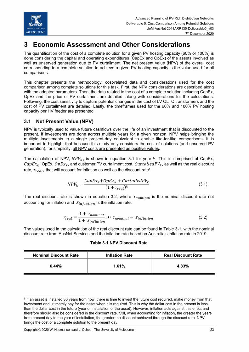


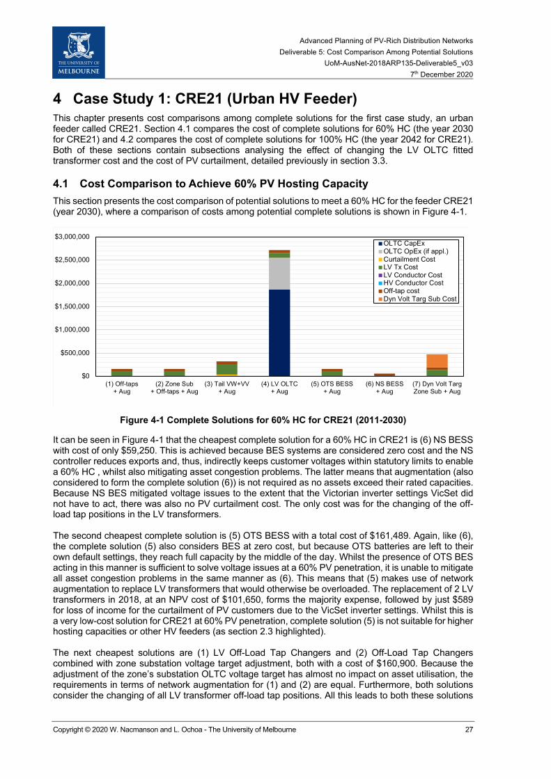
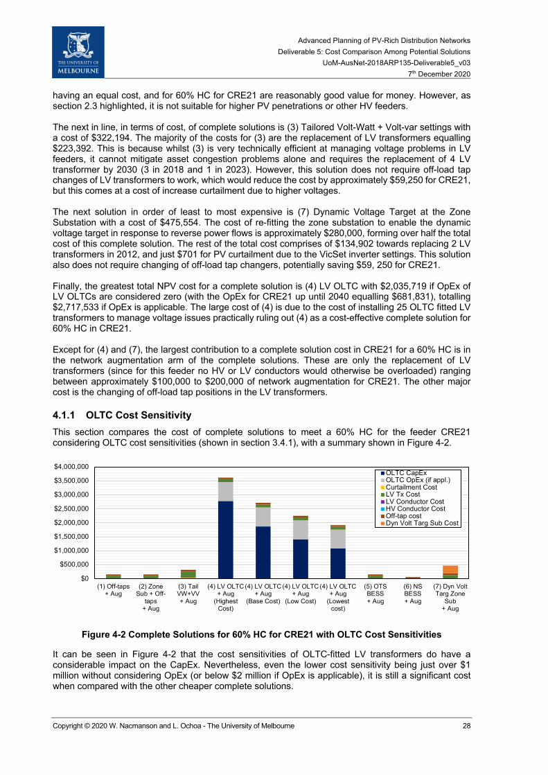


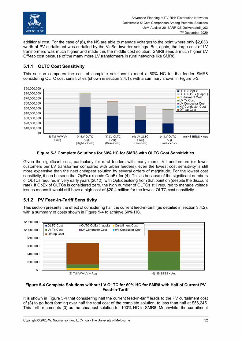


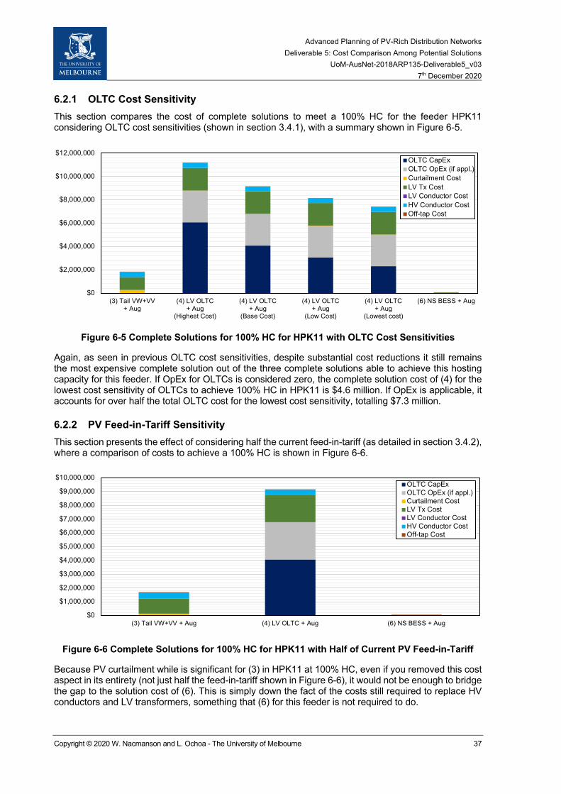


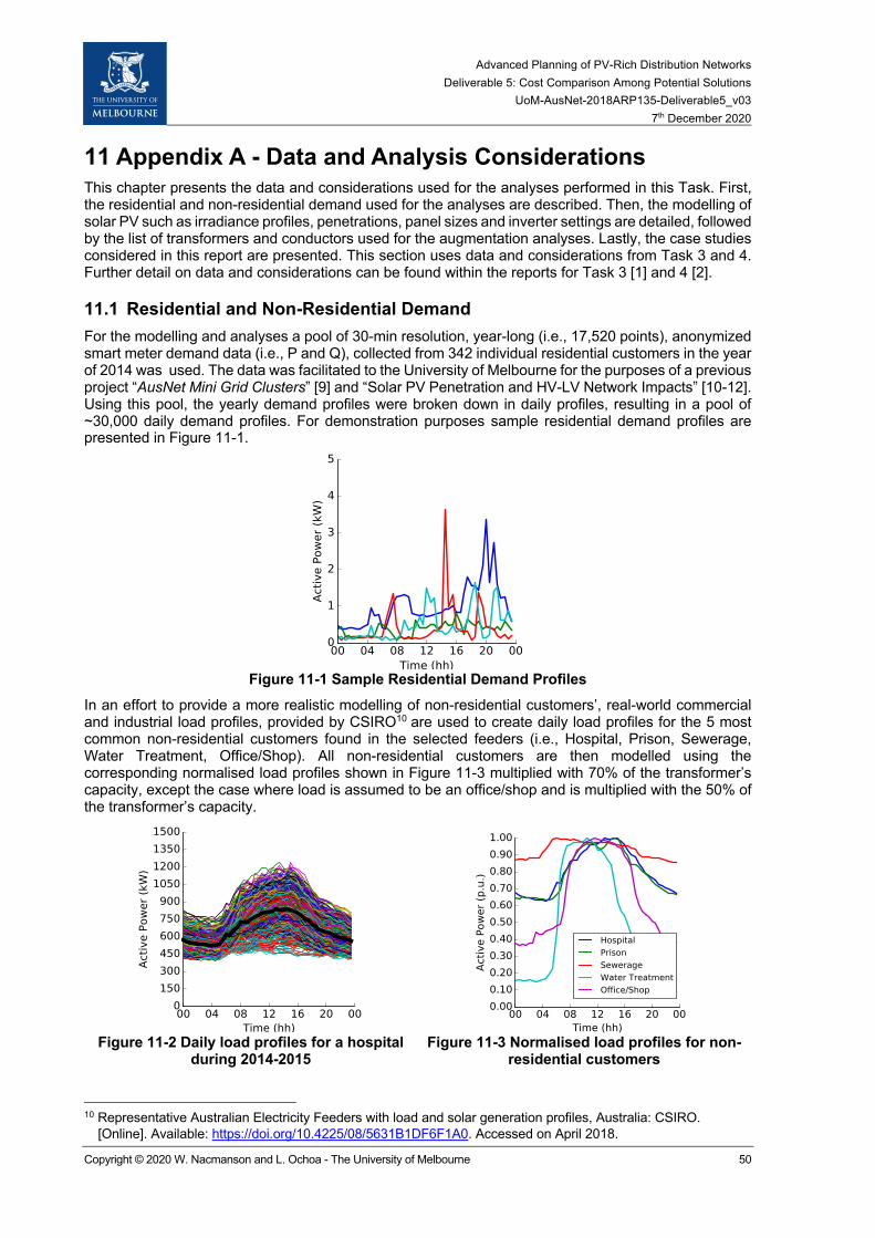


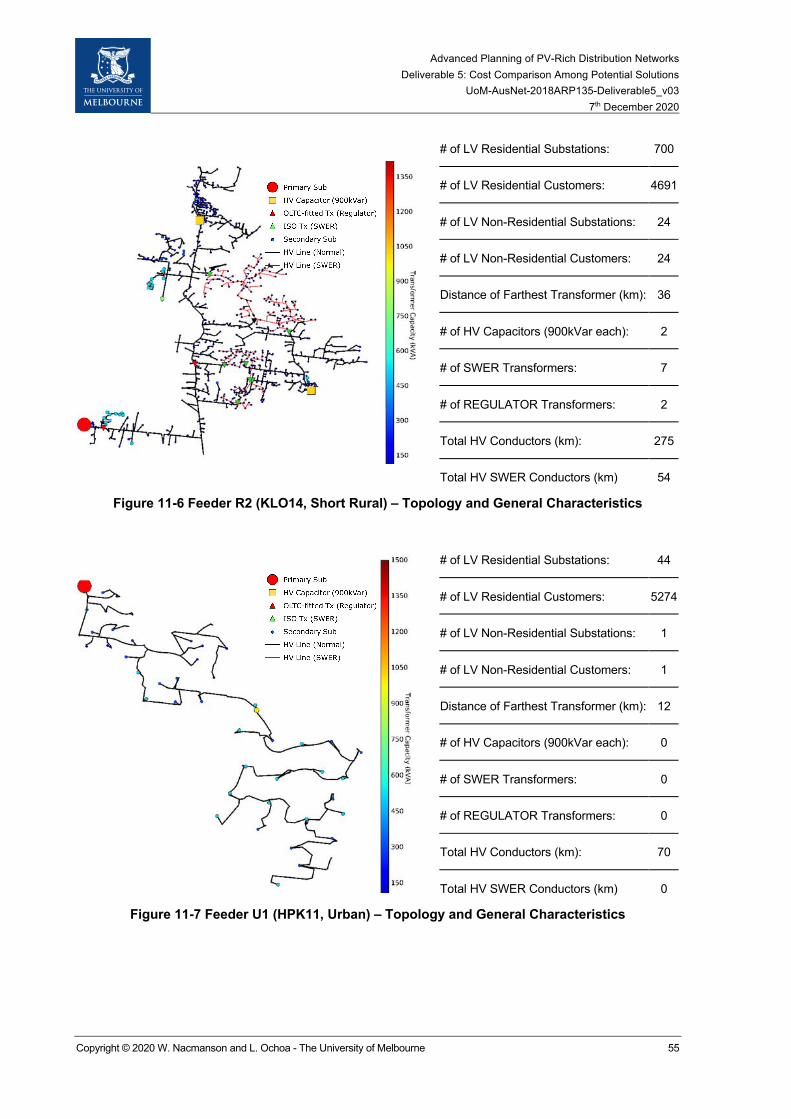


![The Calculation and Analysis of Distribution Network Loss ...distribution network [2]. A method suitable for distribution network line loss analysis with PV power connected is crucial.](https://static.documents.pub/doc/80x56/61150c87b2cda758f4003145/the-calculation-and-analysis-of-distribution-network-loss-distribution-network.jpg)