Advanced Ramsey-based Buchi Automata Inclusion Testing

Parosh Aziz Abdulla1, Yu-Fang Chen2, Lorenzo Clemente3, Lukas Holık1,4,Chih-Duo Hong2, Richard Mayr3, and Tomas Vojnar4

1Uppsala University 2Academia Sinica 3University of Edinburgh4Brno University of Technology

Abstract. Checking language inclusion between two nondeterministic Buchi au-tomata A and B is computationally hard (PSPACE-complete). However, severalapproaches which are efficient in many practical cases have been proposed. Webuild on one of these, which is known as the Ramsey-based approach. It hasrecently been shown that the basic Ramsey-based approach can be drasticallyoptimized by using powerful subsumption techniques, which allow one to prunethe search-space when looking for counterexamples to inclusion. While previousworks only used subsumption based on set inclusion or forward simulation on Aand B , we propose the following new techniques: (1) A larger subsumption rela-tion based on a combination of backward and forward simulations on A and B .(2) A method to additionally use forward simulation between A and B . (3) Ab-straction techniques that can speed up the computation and lead to early detectionof counterexamples. The new algorithm was implemented and tested on automataderived from real-world model checking benchmarks, and on the Tabakov-Vardirandom model, thus showing the usefulness of the proposed techniques.

1 Introduction

Checking inclusion between finite-state models is a central problem in automata theory.First, it is an intriguing theoretical problem. Second, it has many practical applications.For example, in the automata-based approach to model-checking [18], both the systemand the specification are represented as finite-state automata, and the model-checkingproblem reduces to testing whether any behavior of the system is allowed by the speci-fication, i.e., to a language inclusion problem.

We consider language inclusion for Buchi automata (BA), i.e., automata over infi-nite words. While checking language inclusion between nondeterministic BA is com-putationally hard (PSPACE-complete [12]), much effort has been devoted to devisingapproaches that can solve as many practical cases as possible. A naıve approach to lan-guage inclusion between BA A and B would first complement the latter into a BA Bc,and then check emptiness of L(A)∩L(Bc). The problem is that Bc is in general ex-ponentially larger than B . Yet, one can determine whether L(A)∩L(Bc) 6= /0 by onlylooking at some “small” portion of Bc. The Ramsey-based approach [15, 8, 9] gives arecipe for doing this. It is a descendant of Buchi’s original BA complementation proce-dure, which uses the infinite Ramsey theorem in its correctness proof.

The essence of the Ramsey-based approach for checking language inclusion be-tween A and B lies in the notion of supergraph, which is a data-structure representing

a class of finite words sharing similar behavior in the two automata. Ramsey-basedalgorithms contain (i) an initialization phase where a set of supergraph seeds are iden-tified, (ii) a search loop in which supergraphs are iteratively generated by compositionwith seeds, and (iii) a test operation where pairs of supergraphs are inspected for the ex-istence of a counterexample. Intuitively, this counterexample has the form of an infiniteultimately periodic word w1(w2)

ω ∈L(A)∩L(Bc), where one supergraph witnessesthe prefix and the other the loop. While supergraphs themselves are small, and the testin (iii) can be done efficiently, the limiting factor in the basic algorithm lies in theexponential number of supergraphs that need to be generated. Therefore, a crucial chal-lenge in the design of Ramsey-based algorithms is to limit the supergraphs explosionproblem. This can be achieved by carefully designing certain subsumption relations [9,1], which allow one to safely discard subsumed supergraphs, thus reducing the searchspace. Moreover, methods based on minimizing supergraphs [1] by pruning their struc-ture can further reduce the search space, and improve the complexity of (iii) above.

This paper contributes to the Ramsey-based approach to language inclusion in sev-eral ways. (1) We define a new subsumption relation based on both forward and back-ward simulation within the two automata. Our notion generalizes the subset-based sub-sumption of [9] and the forward simulation-based subsumption of [1]. (2) On a similarvein, we improve minimization of supergraphs by employing forward and backwardsimulation for minimizing supergraphs. (3) We introduce a method of exploiting for-ward simulation between the two automata, while previously only simulations internalto each automaton have been considered. (4) Finally, we provide a method to speed upthe tests performed on supergraphs by grouping similar supergraphs together in a com-bined representation and extracting more abstract test-relevant information from it.

The correctness of the combined use of forward and backward simulation turns outto be far from trivial, requiring suitable generalizations of the basic notions of compo-sition and test. Technically, we consider generalized composition and test operationswhere jumps are allowed—a jump occurring between states related by backward sim-ulation. The proofs justifying the use of jumping composition and test are much moreinvolved than in previous works.

We have implemented our techniques and tested them on BA derived from a setof real-world model checking benchmarks [14], and from the Tabakov-Vardi randommodel [17]. The new technique is able to finish many of the difficult problem instancesin minutes, while the algorithm of [1] cannot finish them even in one day. The concretenumbers of our experimental results can be found in Section 8 and also in Appendix H.All the benchmarks we used, the source code, and the executable of our implementationare available at http://www.languageinclusion.org/CONCUR2011.

Related work. An alternative approach to language inclusion for BA is given by rank-based methods [13], which provide a different complementation procedure based ona rank-based analysis of rejecting runs. This approach is orthogonal to Ramsey-basedalgorithms. In fact, while rank-based approaches have a better worst-case complexity,Ramsey-based approaches can still perform better on many examples [9]. A subsumption-based algorithm for the rank-based approach has been given in [4]. Subsumption tech-niques have recently been considered also for automata over finite words [19, 2].

2

2 Preliminaries

A Buchi Automaton (BA) A is a tuple (Σ,Q, I,F,δ) where Σ is a finite alphabet, Q isa finite set of states, I ⊆Q is a non-empty set of initial states, F ⊆Q is a set of acceptingstates, and δ⊆Q×Σ×Q is the transition relation. A run of A on a word w = σ1σ2 . . .∈Σω starting in a state q0 ∈ Q is an infinite sequence q0q1 . . . s.t. (q j−1,σ j,q j) ∈ δ forall j > 0. The run is accepting iff qi ∈ F for infinitely many i. The language of A isL(A) = {w | A has an accepting run on w starting from some q0 ∈ I}.

A path in A on a finite word w = σ1 . . .σn ∈ Σ+ is a finite sequence q0q1 . . .qn s.t.∀0 < j ≤ n : (q j−1,σ j,q j) ∈ δ. The path is accepting iff ∃0 ≤ i ≤ n : qi ∈ F . For anyp,q ∈ Q, let p w

F q iff there is an accepting path on w from p to q, and p w q iff there

is a (not necessarily accepting) path on w from p to q.A forward simulation [3] on A is a relation R ⊆ Q×Q such that pRr only if

p ∈ F =⇒ r ∈ F , and for every transition (p,σ, p′) ∈ δ, there exists a transition(r,σ,r′)∈ δ s.t. p′Rr′. A backward simulation on A ([16], where it is called reverse sim-ulation) is a relation R⊆Q×Q s.t. p′Rr′ only if p′ ∈ F =⇒ r′ ∈ F , p′ ∈ I =⇒ r′ ∈ I,and for every (p,σ, p′) ∈ δ, there exists (r,σ,r′) ∈ δ s.t. pRr. Note that this notion ofbackward simulation is stronger than the usual finite-word automata version, as werequire not only compatibility w.r.t. initial states, but also w.r.t. final states. It can beshown that there exists a unique maximal forward simulation denoted by �A

f and alsoa unique maximal backward simulation denoted by �A

b , which are both polynomial-time computable preorders [10]. We drop the superscripts when no confusion can arise.

In the rest of the paper, we fix two BA A = (Σ,QA , IA ,FA ,δA) and B = (Σ,QB , IB ,FB ,δB). The language inclusion problem consists in deciding whether L(A) ⊆ L(B).It is well known that deciding language inclusion is PSPACE-complete [12], and thatforward simulations [3] can be used as an underapproximation thereof. Here, we focuson deciding language inclusion precisely, by giving a complete algorithm.

3 Ramsey-Based Language Inclusion TestingAbstractly, the Ramsey-based approach for checking L(A)⊆L(B) consists in buildinga finite set X ⊆ 2L(A) of fragments of L(A) satisfying the following two properties:α (covering)

⋃X = L(A).

β (dichotomy) For all X ∈ X , either X ⊆ L(B) or X ∩L(B) = /0.

The covering property ensures that the considered fragments cover L(A), and the di-chotomy property states that the fragments are either entirely in L(B) or disjoint fromL(B). Moreover, the fragments are chosen such that they can be effectively generatedand such that their inclusion in L(B) is easy to test. During the generation of the frag-ments, it then suffices to test each of them for inclusion in L(B). If this is the case, theinclusion L(A) ⊆ L(B) holds. Otherwise, there is a fragment X ⊆ L(A) \L(B) s.t.every ω-word w ∈ X is a counterexample to the inclusion of L(A) in L(B).

We now instantiate the above described abstract algorithm by giving primitives forrepresenting fragments of L(A) satisfying the conditions of covering and dichotomy.Much like in [8], we introduce the notion of arcs for satisfying Condition α, the notionof graphs for Condition β, and then we put them together in the notion of supergraphsas to satisfy α+β. Then, we explain that supergraphs can be effectively generated andthat the fragment languages they represent can be easily tested for inclusion in L(B).

3

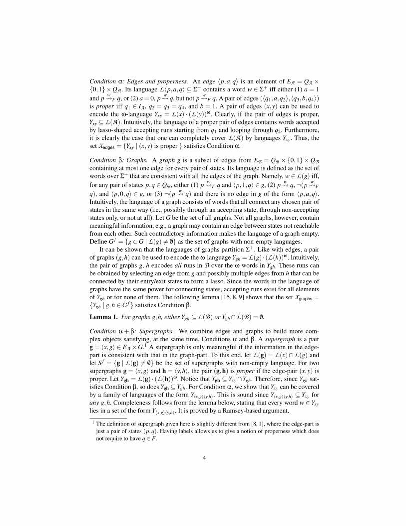
Condition α: Edges and properness. An edge 〈p,a,q〉 is an element of EA = QA ×{0,1}×QA . Its language L〈p,a,q〉 ⊆ Σ+ contains a word w ∈ Σ+ iff either (1) a = 1and p w

F q, or (2) a = 0, p w q, but not p w

F q. A pair of edges (〈q1,a,q2〉,〈q3,b,q4〉)is proper iff q1 ∈ IA , q2 = q3 = q4, and b = 1. A pair of edges (x,y) can be used toencode the ω-language Yxy = L(x) · (L(y))ω. Clearly, if the pair of edges is proper,Yxy ⊆ L(A). Intuitively, the language of a proper pair of edges contains words acceptedby lasso-shaped accepting runs starting from q1 and looping through q2. Furthermore,it is clearly the case that one can completely cover L(A) by languages Yxy. Thus, theset Xedges = {Yxy | (x,y) is proper } satisfies Condition α.

Condition β: Graphs. A graph g is a subset of edges from EB = QB ×{0,1}×QBcontaining at most one edge for every pair of states. Its language is defined as the set ofwords over Σ+ that are consistent with all the edges of the graph. Namely, w ∈ L(g) iff,for any pair of states p,q ∈QB , either (1) p w

F q and 〈p,1,q〉 ∈ g, (2) p w q, ¬(p w

F

q), and 〈p,0,q〉 ∈ g, or (3) ¬(p w q) and there is no edge in g of the form 〈p,a,q〉.

Intuitively, the language of a graph consists of words that all connect any chosen pair ofstates in the same way (i.e., possibly through an accepting state, through non-acceptingstates only, or not at all). Let G be the set of all graphs. Not all graphs, however, containmeaningful information, e.g., a graph may contain an edge between states not reachablefrom each other. Such contradictory information makes the language of a graph empty.Define G f = {g ∈ G | L(g) 6= /0} as the set of graphs with non-empty languages.

It can be shown that the languages of graphs partition Σ+. Like with edges, a pairof graphs (g,h) can be used to encode the ω-language Ygh = L(g) · (L(h))ω. Intuitively,the pair of graphs g, h encodes all runs in B over the ω-words in Ygh. These runs canbe obtained by selecting an edge from g and possibly multiple edges from h that can beconnected by their entry/exit states to form a lasso. Since the words in the language ofgraphs have the same power for connecting states, accepting runs exist for all elementsof Ygh or for none of them. The following lemma [15, 8, 9] shows that the set Xgraphs ={Ygh | g,h ∈ G f } satisfies Condition β.

Lemma 1. For graphs g,h, either Ygh ⊆ L(B) or Ygh∩L(B) = /0.

Condition α + β: Supergraphs. We combine edges and graphs to build more com-plex objects satisfying, at the same time, Conditions α and β. A supergraph is a pairg = 〈x,g〉 ∈ EA ×G.1 A supergraph is only meaningful if the information in the edge-part is consistent with that in the graph-part. To this end, let L(g) = L(x)∩L(g) andlet S f = {g | L(g) 6= /0} be the set of supergraphs with non-empty language. For twosupergraphs g = 〈x,g〉 and h = 〈y,h〉, the pair (g,h) is proper if the edge-pair (x,y) isproper. Let Ygh = L(g) · (L(h))ω. Notice that Ygh ⊆ Yxy∩Ygh. Therefore, since Ygh sat-isfies Condition β, so does Ygh ⊆Ygh. For Condition α, we show that Yxy can be coveredby a family of languages of the form Y〈x,g〉〈y,h〉. This is sound since Y〈x,g〉〈y,h〉 ⊆ Yxy forany g,h. Completeness follows from the lemma below, stating that every word w ∈ Yxylies in a set of the form Y〈x,g〉〈y,h〉. It is proved by a Ramsey-based argument.

1 The definition of supergraph given here is slightly different from [8, 1], where the edge-part isjust a pair of states (p,q). Having labels allows us to give a notion of properness which doesnot require to have q ∈ F .

4

Lemma 2. For proper edges (x,y) and w∈Yxy, there exist graphs g,h s.t. w∈Y〈x,g〉〈y,h〉.

Thus, Yxy can be covered by Xxy = {Ygh | g,h ∈ G f ,g = 〈x,g〉,h = 〈y,h〉}. SinceXedges covers L(A), and each Yxy ∈ Xedges can be covered by Xxy, it follows that X ={Ygh | g,h ∈ S f ,(g,h) is proper} covers L(A). Thus, X fulfills α+β.

Generating and Testing Supergraphs. While supergraphs in S f are a convenient syn-tactic object for manipulating languages in X , testing that a given supergraph has non-empty language is expensive (PSPACE-complete). In [11], this problem is elegantlysolved by introducing a natural notion of composition of supergraphs, which preservesnon-emptiness: The idea is to start with a (small) set of supergraphs which have non-empty language by construction, and then to obtain S f by composing supergraphs untilno more supergraphs can be generated.

For a BA C and a symbol σ∈ Σ, let Eσ

C = {〈p,a,q〉 | (p,σ,q)∈ δC ,(a = 1 ⇐⇒ p∈F ∨q ∈ F)} be the set of edges induced by σ. The initial seed for the procedure is givenby one-letter supergraphs in S1 =

⋃σ∈Σ{(x,Eσ

B) | x ∈ Eσ

A}. Notice that S1 ⊆ S f by con-struction. Next, two edges x = 〈p,a,q〉 and y = 〈q′,b,r〉 are composable iff q = q′. Forcomposable edges x and y, let x;y = 〈p,max(a,b),r〉. Further, the composition g;h ofgraphs g and h is defined as follows: 〈p,c,r〉 ∈ g;h iff there is a state q s.t. 〈p,a,q〉 ∈ gand 〈q,b,r〉 ∈ h, and c = maxq∈Q{max(a,b) | 〈p,a,q〉 ∈ g,〈q,b,r〉 ∈ h}. Then, super-graphs g = 〈x,g〉 and h = 〈y,h〉 are composable iff 〈x,y〉 are composable, and theircomposition is the supergraph g;h = 〈x;y,g;h〉. Notice that S f is closed under compo-sition, i.e., g,h∈S f =⇒ g;h∈S f . Composition is also complete for generating S f :

Lemma 3. [1] A supergraph g is in S f iff ∃g1, . . . ,gn ∈ S1 such that g = g1; . . . ;gn.

Now that we have a method for generating all relevant supergraphs, we need a wayof checking inclusion of (supergraphs representing) fragments of L(A) in L(B). Let(g,h) be a (proper) pair of supergraphs. By the dichotomy property, Ygh ⊆ L(B) iffYgh∩L(B) 6= /0. We test the latter condition by the so-called double graph test: For a pairof supergraphs (g,h), DGT(g,h) iff, whenever (g,h) is proper, then LFT(g,h). Here,LFT is the so-called lasso-finding test: Intuitively, LFT checks for a lasso with a handlein g and an accepting loop in h. Formally, LFT(g,h) iff there is an edge 〈p,a0,q0〉 ∈ gand an infinite sequence of edges 〈q0,a1,q1〉, 〈q1,a2,q2〉, . . . ∈ h s.t. p ∈ I and a j = 1for infinitely many j’s.

Lemma 4. [1] L(A)⊆ L(B) iff for all g,h ∈ S f , DGT(g,h).

Basic Algorithm [8]. The basic algorithm for checking inclusion enumerates all super-graphs from S f by extending supergraphs on the right by one-letter supergraphs fromS1; that is, a supergraph g generates new supergraphs by selecting some h ∈ S1 andbuilding g;h. Then, L(A)⊆ L(B) holds iff all the generated pairs pass the DGT.

Intuitively, the algorithm processes all lasso-shaped runs that can be used to acceptsome words in A . These runs are represented by the edge-parts of proper pairs of gen-erated supergraphs. For each such run of A , the algorithm uses LFT to test whetherthere is a corresponding accepting run of B among all the possible runs of B on thewords represented by the given pair of supergraphs. These latter runs are encoded bythe graph-parts of the respective supergraphs.

5

4 Optimized Language Inclusion Testing

The basic algorithm of Section 3 is wasteful for two reasons. First, not all edges in thegraph component of a supergraph are needed to witness a counterexample to inclusion:Hence, we can reduce a graph by keeping only a certain subset of its edges (Optimiza-tion 1). Second, not all supergraphs need to be generated and tested: We show a methodwhich safely allows the algorithm to discard certain supergraphs (Optimization 2). Bothoptimizations rely on various notions of subsumption, which we introduce next.

Given two edges x = 〈p,a,q〉 and y = 〈r,b,s〉, we say that y subsumes x, writtenx v y, if p = r, a ≤ b, and q = s; that x forward-subsumes y, written x vf y, if p = r,a ≤ b, and q �f s; that x backward-subsumes y, written x vb y, if p �b r, a ≤ b, andq = s; and that x forward-backward-subsumes y, written x vfb y, if p �b r, a ≤ b, andq�f s. We lift all the notions of subsumption to graphs: For any z ∈ {f,b, fb, } and forgraphs g and h, let gvz h iff, for every edge x ∈ g, there exists an edge y ∈ h s.t. xvz y.Since the simulations �f and �b are preorders, all subsumptions are preorders. Wedefine backward and forward-backward subsumption equivalence as 'b = vb ∩v−1

b

and 'fb =vfb∩v−1fb , respectively.

4.1 Optimization 1: Minimization of SupergraphsThe first optimization concerns the structure of individual supergraphs. Let g = 〈x,g〉 ∈S be a supergraph, with g its graph-component. We minimize g by deleting edges thereinwhich are subsumed byvfb-larger ones. That is, whenever we have xvfb y for two edgesx,y ∈ g, we remove x and keep y. Intuitively, subsumption-larger arcs contribute moreto the capability of representing lassoes since their right and left endpoints are �f /�b-larger, respectively, and have therefore a richer choice of possible futures and pasts.Subsumption smaller arcs are thus redundant, and removing them does not change thecapability of g to represent lassoes in B . Formally, we define a minimization operationMin mapping a supergraph g = 〈x,g〉 to its minimized version Min(g) = 〈x,Min(g)〉where Min(g) is the minimization applied to the graph-component.2

Definition 1. For two graphs g and h, let g 6 h iff (1) g v h and (2) h vfb g. Forsupergraphs g = 〈x,g〉 and h = 〈y,h〉, let g 6 h iff x = y and g 6 h. A minimization ofgraphs is any function Min such that, for any graph h, Min(h)6 h.

Point 1 in the definition of6 allows some edges to be erased or their label decreased.Point 2 states that only subsumed arcs can be removed or have their label decreased.Note also that, clearly, Min(h)6 h holds for any supergraph h. Finally, note that Min isnot uniquely determined: First, there are many candidates satisfying Min(h) 6 h. Yet,an implementation will usually remove a maximal number of edges to keep the size ofgraphs to a minimum. Second, even if we required Min(h) to be a 6-smallest element(i.e., no further edge can be removed), the minimization process might encounter vfb-equivalent edges, and in this case, we do not specify which ones get removed. Therefore,we prove correctness for any minimization satisfying Min(h)6 h.

Intuitively, a minimized supergraph g can be seen as a small representative of allsupergraphs h ∈ G f with g 6 h, and of all the fragments of L(A) encoded by them.

2 In [1], we used vf for minimization. The theory allowing the use of vfb is significantly moreinvolved, but as as shown in Section 8, the use ofvfb turns out to be much more advantageous.

6

Using representatives allows us to deal with a smaller number of smaller supergraphs.We now explain how (sufficiently many) representatives encoding fragments of L(A)can be generated and tested for inclusion in L(B).

Generating representatives of supergraphs. We need to create a representative of eachsupergraph in S f by composing representatives only. Let g= 〈x,g〉 and h= 〈y,h〉 be twocomposable supergraphs, representing g′ = 〈x,g′〉 and h′ = 〈y,h′〉, respectively. If graphcomposition were 6-monotone, i.e., g;h 6 g′;h′, then we would be done. However,graph composition is not monotone: The reason is that some composable edges e ∈ g′

and f ∈ h′ may be erased by minimization, and be represented by some e ∈ g and f ∈ hinstead, with e vfb e and f vfb f . But now, e and f are not necessarily composableanymore. Thus, g;h 66 g′;h′. We solve this problem in two steps: We allow compositionto jump to �b-larger states (Def. 2), and relax the notion of representative (Def. 3).

Definition 2. Given graphs g,h ∈ G, their jumping composition g #b h contains anedge 〈p,c,r〉 ∈ g #b h iff there are edges 〈p,a,q〉 ∈ g, 〈q′,b,r〉 ∈ h s.t. q �b q′, andc = maxq,q′{max(a,b) | 〈p,a,q〉 ∈ g,〈q′,b,r〉 ∈ h,q�b q′}. For two composable super-graphs g = 〈x,g〉 and h = 〈y,h〉, let g #b h = 〈x;y,g #b h〉.

Jumping composition alone does not yet give the required monotonicity property.The problem is that g #b h is not necessarily a minimized version of g′;h′, but it is only aminimized version of something 'b-equivalent to g′;h′. This leads us to the followingmore liberal notion of representatives, which is based on6modulo the equivalence'b,and for which Lemma 5 proves the required monotonicity property.

Definition 3. A graph g ∈ G is a representative of a graph h ∈ G f , denoted g E h, iffthere exists h ∈ G such that g 6 h 'b h. For supergraphs g = 〈x,g〉,h = 〈y,h〉 ∈ S, wesay that g is a representative of h, written gE h, iff x = y and gE h. Let SR = {g | ∃h ∈S f . gE h} be the set of representatives of supergraphs.

Lemma 5. For supergraphs g,h ∈ SR and g′,h′ ∈ S f , if g E g′, h E h′ and g′,h′ arecomposable, then g,h are composable and g #b hE g′;h′ and g #b h ∈ SR.

Lemma 6. Let f∈ S, g∈ SR, and h∈ S f . If f6 g and gE h, then fE h (and thus f∈ SR).In particular, the statement holds when f = Min(g).

Lemmas 5, 6, and 3 imply that creating supergraphs by #b-composing represen-tatives, followed by further minimization, suffices to create a representative of eachsupergraph in S f . This solves the problem of generating representatives of supergraphs.

Weak properness and Relaxed DGT. We now present a relaxed DGT proposed in [1],which we further improve below. The idea is to weaken the properness condition inorder to allow more pairs of supergraphs to be eligible for LFT on their graph part. Thismay lead to a quicker detection of a counterexample. Weak properness is sound sinceit still produces fragments Ygh ⊆ L(A) as required by Condition α. Completeness isguaranteed since properness implies weak properness.

Definition 4. (adapted from [1]) A pair of edges (〈p,a,q〉,〈r,b,s〉) is weakly proper iffp ∈ IA , r �f q, r �f s, and b = 1,3 and a pair of supergraphs (g = 〈x,g〉,h = 〈y,h〉) is3 We note that instead of testing r �f q, testing inclusion of the languages of the states is suf-

ficient. Furthermore, instead of testing r �f s, one can test for delayed simulation, but not forlanguage inclusion. See Lemma 34 in Appendix C.

7

weakly proper when (x,y) is weakly proper. Supergraphs g,h pass the relaxed doublegraph test, denoted RDGT(g,h), iff whenever (g,h) is weakly proper, then LFT(g,h).

Lemma 7. [1] L(A)⊆ L(B) iff for all g,h ∈ S f , RDGT(g,h).

Testing representatives of supergraphs. We need a method for testing inclusion in L(B)of the fragments of L(A) encoded by representatives of supergraphs that is equivalentto testing inclusion of fragments of L(A) encoded by the represented supergraphs. Aswith composition, minimization is not compatible with such testing since edges neededto find loops may be erased during the minimization process. Technically, this resultsin the LFT (and therefore RDGT) not being E-monotone. Therefore, we generalizethe LFT by allowing jumps to �b-larger states, in a similar way as with #b. Lemma 8establishes the required monotonicity property.

Definition 5. A pair of graphs (g,h) passes the jumping lasso-finding test, denotedLFTb(g,h), iff there is an edge 〈p,a0,q0〉 in g and an infinite sequence of edges 〈q′0,a1,q1〉,〈q′1,a2,q2〉, . . . in h s.t. p ∈ I, qi �b q′i for all i ≥ 0, and a j = 1 for infinitely many j’s.A pair of supergraphs (g,h) passes the jumping relaxed double graph test, denotedRDGTb(g,h), iff whenever (g,h) is weakly proper, then LFTb(g,h).

Lemma 8. For any g,h ∈ SR and g′,h′ ∈ S f such that g E g′ and h E h′, it holds thatRDGTb(g,h)⇐⇒ RDGT(g′,h′).

Algorithm with minimization. By Lemma 8, RDGTb on representatives is equivalentto RDGT on the represented supergraphs. Together with Lemma 7, this means that itis enough to generate a representative of each supergraph from S f , and test all pairsof the generated supergraphs with RDGTb. Thus, we have obtained a modification ofthe basic algorithm which starts from minimized 1-letter supergraphs in Min(S1) ={Min(g) | g ∈ S1}, and constructs new supergraphs by #b-composing already generatedsupergraphs with Min(S1) on the right. New supergraphs are further minimized withMin. Inclusion holds iff all pairs of generated supergraphs pass RDGTb.

4.2 Optimization 2: Discarding Subsumed Supergraphs

The second optimization gives a rule for discarding supergraphs subsumed by someother supergraph. This is safe in the sense that if a subsumed supergraph can yielda counterexample to language inclusion, then also the subsuming one can yield a coun-terexample. We present an improved version of the subsumption from [1]. The newversion uses both �f and �b on the B part of supergraphs instead of �f only. This al-lows us to discard significantly more supergraphs than in [1], as illustrated in Section 8.

Definition 6. We say that a supergraph g = 〈x,g〉 subsumes a supergraph g′ = 〈y,g′〉,written gvfb g′, iff yvf x and gvfb g′.

Intuitively, if y vf x, then x has more power for representing lassoes in A than ysince, by the properties of forward simulation, it has a richer choice of possible for-ward continuations in A . On the other hand, gvfb g′ means that g′ has more chance ofrepresenting lassoes in B than g: In fact, g′ contains edges that have a richer choice ofbackward continuations (due to the �b on the left endpoints of the edges) as well as

8

a richer choice of forward continuations (due to the �f on the right endpoints). Thus, itis more likely for g than for g′ to lead to a counterexample to language inclusion. Thisintuition is confirmed by the lemma below, stating the vfb-monotonicity of RDGTb.

Lemma 9. For supergraphs g,h ∈ SR and g′,h′ ∈ S, if g vfb g′ and h vfb h′, thenRDGTb(g,h)⇒ RDGTb(g′,h′).

Therefore, no counterexample is lost by testing only vfb-smaller supergraphs. Toshow that we can completely discardvfb-larger supergraphs, we need to show that sub-sumption is compatible with composition, i.e., that descendants of larger supergraphsare (eventually) subsumed by descendants of smaller ones. Ideally, we would achievethis by showing the following more general fact: For two composable representativesg′,h′ ∈ SR that are subsumed by supergraphs g and h, respectively, the composite su-pergraph g #b h subsumes g′ #b h′. The problem is that subsumption does not preservecomposability: Even if g′,h′ are composable, this needs not to hold for g,h.

We overcome this difficulty by taking into account the specific way supergraphsare generated by the algorithm. Since we only generate new supergraphs by composingold ones on the right with 1-letter minimized supergraphs, we do not need to showthat arbitrary composition is vfb-monotone. Instead, we show that, for representativesg,g′ ∈ SR and a 1-letter minimized supergraph h′ ∈ Min(S1), if g subsumes g′, thenthere will always be a supergraph h available which is composable with g such thatg #b h subsumes g′ #b h′. Thus, we can safely discard g′ from the rest of the computation.

Lemma 10. For any g,g′ ∈ SR with g vfb g′ and h′ ∈ Min(S1) such that g′ and h′are composable, there exists h ∈ Min(S1) such that for all h ∈ SR with h vfb h, g iscomposable with h and g #b hvfb g′ #b h′.

Algorithm with minimization and subsumption. We have obtained a modification ofthe algorithm with minimization. It starts with a subset Init⊆Min(S1) of vfb-smallestminimized one-letter supergraphs. New supergraphs are generated by #b-compositionon the right with supergraphs in Init, followed by minimization with Min. Generatedsupergraphs that are vfb-larger than other generated supergraphs are discarded. Theinclusion holds iff all pairs of generated supergraphs that are not discarded pass RDGTb.(An illustration of a run of the algorithm can be found in Appendix D.)

5 Using Forward Simulation Between A and BPreviously, we showed that some supergraphs can safely be discarded because somevfb-smaller ones are retained, which preserves the chance to find a counterexample tolanguage inclusion. Our subsumption relation vfb is based on forward/backward simu-lation on A and B . In order to use forward simulation between A and B , we describea different reason to discard supergraphs. Generally, supergraphs can be discarded be-cause they can neither find a counterexample to inclusion (i.e., always pass the RDGT)nor generate any supergraph that can find a counterexample. However, the RDGT isasymmetric w.r.t. the left and right supergraph. Thus, a supergraph that is useless (i.e.,not counterexample-finding) in the left role is not necessarily useless in the right role(and vice-versa). The following condition C is sufficient for a supergraph to be uselesson the left. Moreover, C is efficiently computable and compatible with subsumption.Therefore, its use preserves the soundness and completeness of our algorithm.

9

Definition 7. For g=〈〈p,a,q〉,g〉 ∈ S, C(g) iff p /∈ IA ∨(∃〈r,b,s〉 ∈ g. r ∈ IB ∧q�ABf s).

The first part p /∈ IA of the condition is obvious because paths witnessing coun-terexamples to inclusion must start in an initial state. The second part (∃〈r,b,s〉 ∈ g. r ∈IB ,q�AB

f s) uses forward-simulation�ABf between A and B to witness that neither this

supergraph nor any other supergraph generated from it will find a counterexample whenused on the left side of the RDGT. It might still be needed for tests on the right side ofthe RDGT though. Instead of �AB

f , every relation implying language inclusion wouldsuffice, but (as mentioned earlier) simulation preorder is efficiently computable whileinclusion is PSPACE-complete. The following lemma shows the correctness of C.

Lemma 11. ∀g,h ∈ SR. C(g)⇒ RDGTb(g,h).

C is vfb-upward-closed and closed w.r.t. right extensions. Hence, it is compatiblewith subsumption-based pruning of the search space and with the employed incremen-tal construction of supergraphs (namely, satisfaction of the condition is inherited tosupergraphs newly generated by right extension with one-letter supergraphs).

Lemma 12. Let g,h ∈ S s.t. gvfb h. Then C(g)⇒ C(h).

Lemma 13. Let g ∈ SR, h ∈Min(S1) be composable. Then C(g)⇒ C(g #b h).

In principle, one could store separate sets of supergraphs for use on the left/rightin the RDGT, respectively. However, since all supergraphs need to be used on the rightanyway, a simple flag is more efficient. We assign the label L to a supergraph to indi-cate that it is still useful on the left in the RDGT. If a supergraph satisfies condition C,then the L-label is removed. The algorithm counts the number of stored supergraphsthat still carry the L-label. If this number drops to zero, then (1) it will remain zero(by Lemma 13), and (2) no RDGT will ever find a counterexample: In this case, thealgorithm can terminate early and report inclusion. In the special case where forward-simulation holds even between the initial states of A and B , condition C is true for everygenerated supergraph. Thus, all L-labels are removed and the algorithm terminates im-mediately, reporting inclusion. Of course, condition C can also help in other cases wheresimulation does not hold between initial states but “more deeply” inside the automata.

The following lemma shows that if some supergraph g can find a counterexamplewhen used on the left in the RDGT, then at least one of its 1-letter right-extensionscan also find a counterexample. Intuitively, the counterexample has the form of a prefixfollowed by an infinite loop, and the prefix can always be extended by one step. E.g., theinfinite words xy(abc)ω and xya(bca)ω are equivalent. This justifies the optimization inline 15 of our algorithm (see Appendix G).

Lemma 14. Let g,h ∈ SR. If ¬RDGTb(g,h), then there exists a vfb-minimal super-graph f in Min(S1) and e ∈ SR s.t. ¬RDGTb(g #b f,e).4

4 A slightly modified version, Lemma 37 in Appendix E, holds for the version of the RDGTmentioned in the footnote on Definition 4.

10

6 Metagraphs and a New RDGT

Since many supergraphs share the same graph for B , they can be more efficiently repre-sented by a combined structure that we call a metagraph. Moreover, metagraphs allowto define a new RDGT where several A-edges jointly witness a counterexample to in-clusion, so that counterexamples can be found earlier than with individual supergraphs.

A metagraph is a structure (X ,g) where X ⊆ EA is a set of A-edges and g∈GB . Themetagraph (X ,g) represents the set of all supergraphs 〈x,g〉 with x ∈ X . The L-labels ofsupergraphs then become labels of the elements of X since the graph g is the same.

We lift basic concepts from supergraphs to metagraphs. For every character σ ∈ Σ,there is exactly one single-letter metagraph (Eσ

A ,Eσ

B). Let M1 = {(Eσ

A ,Eσ

B)| σ ∈ Σ}.Thus, the set of single-letter metagraphs M1 represents all single-letter supergraphsin S1. The function RightExtend defines the composition of two metagraphs such thatRightExtend((X ,g),(Y,h))= (X ;Y,g#bh), which is the metagraph containing the super-graphs that are #b-right extensions of supergraphs contained in (X ,g) by supergraphscontained in (Y,h). The L-labels of the elements z ∈ X ;Y are assigned after testingcondition C. The function Minf is defined on sets X ⊆ EA s.t. Minf(X) contains the vf -minimal edges of X . If some edges are vf -equivalent, then Minf(X) contains just anyof them. Let MinM(X ,g) = (Minf(X),Min(g)). Thus, MinM(X ,g) contains exactly onerepresentative of every 'fb equivalence class of the vfb-minimal supergraphs in (X ,g).

It is not meaningful to define subsumption for metagraphs. Instead, we need to re-move certain supergraphs (i.e., A-edges) from some metagraph if another metagraphcontains avfb-smaller supergraph. If no A-edge remains, i.e., X = /0 in (X ,g), then thismetagraph can be discarded. This is the purpose of introducing the function Clean: Ittakes two metagraphs (X ,g) and (Y,h), and it returns a metagraph (Z,g) that describesall supergraphs from (X ,g) for which there is no vfb-smaller supergraph in (Y,h). For-mally, if hvfb g, then x ∈ Z iff x ∈ X and 6 ∃y ∈Y s.t. xvf y. Otherwise, if h 6vfb g, thenZ = X . Now we define a generalized RDGT on metagraphs.

Definition 8. A pair of sets of A-edges X ,Y ⊆ EA passes the forward-downward jump-ing lasso-finding test, denoted LFTf(X ,Y ), iff there is an arc 〈p,a0,q0〉 in X (with theL-label) and an infinite sequence of arcs 〈q′0,a1,q1〉,〈q′1,a2,q2〉, . . . in Y s.t. p ∈ IA ,q′i �f qi for all i≥ 0, and a j = 1 for infinitely many j’s.

Definition 9. RDGTMb ((X,g),(Y,h)) iff, whenever LFTf(X ,Y ), then LFTb(g,h).

The following lemma shows the soundness of the new RDGT.

Lemma 15. Let (X ,g),(Y,h) be metagraphs where all contained supergraphs are inSR. If ¬RDGTM

b ((X,g),(Y,h)), then L(A) 6⊆ L(B).

If there are x ∈ X ,y ∈ Y s.t. ¬RDGTb(〈x,g〉,〈y,h〉), then ¬RDGTMb ((X,g),(Y,h)),

by Definitions 4, 8, and 9. Thus the completeness of the new RDGT follows alreadyfrom Lemmas 7 and 8. Checking RDGTM

b ((X,g),(Y,h)) can be done very efficientlyfor large numbers of metagraphs, by using an abstraction technique that extracts test-relevant information from the metagraphs and stores it separately (see Appendix G).

11

7 The Main AlgorithmAlgorithm 1 describes our inclusion testing algorithm. The function Clean is extendedto sets of metagraphs in the standard way and implemented in procedures Clean1 andClean3 in which the result overwrites the first argument (the two procedures differ in therole of the first argument, and Clean3 in addition discards empty metagraphs). Lines 1-6compute the metagraphs which contain the subsumption-minimal 1-letter supergraphs.Lines 7-10 initialize the set Next with these metagraphs and assign the correct labelsby testing condition C. L(x) denotes that the A-arc x is labeled with L. Lines 11-21describe the main loop. It runs until Next is empty or there are no more L-labels left.In the main loop, metagraphs are tested (lines 13-14) and then moved from Next toProcessed without the L-label (line 15). Moreover, new metagraphs are created andsome parts of them discarded by the Clean operation (lines 16-21). Extra bookkeepingis needed to handle the case where L-labels are regained by supergraphs in Processedin line 19 (see Clean2 in Appendix F).

Algorithm 1: Inclusion Checking with MetagraphsInput: BA A = (Σ,QA , IA ,FA ,δA ), B = (Σ,QB , IB ,FB ,δB ), and the set M1

A ,B .Output: TRUE if L(A)⊆ L(B). Otherwise, FALSE.Next := {MinM((X ,g)) | (X ,g) ∈M1

A ,B}; Init := /0;1

while Next 6= /0 do2Pick and remove a metagraph (X ,g) from Next;3Clean1((X ,g), Init);4if X 6= /0 then5

Clean3(Init,(X ,g)); Add (X ,g) to Init;6

Processed := /0; Next := Init;7foreach (X ,g) ∈ Next do8

foreach x ∈ X do9if ¬C(〈x,g〉) then label x with L10

while Next 6= /0∧∃(X ,g) ∈ Next∪Processed. ∃x ∈ X .L(x) do11Pick a metagraph (X ,g) from Next and remove (X ,g) from Next;12

if ¬RDGTMb ((X,g),(X,g)) then return FALSE ;13

if ∃(Y,h) ∈ Processed : ¬RDGTMb ((Y,h),(X,g))∨¬RDGTM

b ((X,g),(Y,h)) then14return FALSE ;Create (X ′,g) from (X ,g) by removing the L-labels from X and add (X ′,g) to15Processed;foreach (Y,h) ∈ Init do16

(Z, f ) := MinM(RightExtend((X ,g),(Y,h)));17if Z 6= /0 then Clean1((Z, f ),Next);18if Z 6= /0 then Clean2((Z, f ),Processed);19if Z 6= /0 then20

Clean3(Next,(Z, f )); Clean3(Processed,(Z, f )); Add (Z, f ) to Next;21

return TRUE ;22

Theorem 1. Algorithm 1 terminates. It returns TRUE iff L(A)⊆ L(B).

12

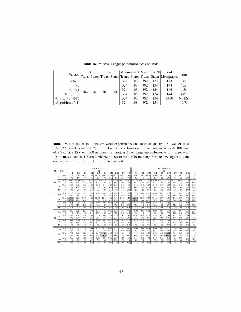
Table 1. Language inclusion checking on mutual exclusion protocols. Forward simulation holdsbetween initial states. The option -c is extremely effective in such cases.

ProtocolA B Algorithm New Algorithm

Trans. States Trans. States of [1] default -b -b -qr -b -qr -cPeterson 33 20 34 20 0.46s 0.39s 0.54 0.61s 0.03sPhils 49 23 482 161 12h36m 11h3m 7h21m 7h23m 0.1sMcs 3222 1408 21503 7963 >24h 2m43s 2m32s 2m49s 1m24sBakery 2703 1510 2702 1509 >24h >24h >24h >24h 12sFischer 1395 634 3850 1532 4h50m 2m38s 2m50s 27s 3.6sFischerV2 147 56 147 56 13m15s 5m14s 1m26s 1m1s 0.1s

Table 2. Language inclusion checking on mutual exclusion protocols. Language inclusion holds,but forward simulation does not hold between initial states (we call this category “inclusion”).The new alg. is much better in FischerV3, due to metagraphs. Option -b is effective in FischerV4.BakeryV2 is a case where -c is useful even if simulation does not hold between initial states.

ProtocolA B Algorithm New Algorithm

Trans. States Trans. States of [1] default -b -b -qr -b -qr -cFischerV3 1400 637 1401 638 3h6m 45s 10s 11s 7sFischerV4 147 56 1506 526 >24h >24h 1h31m 2h12m 2h12mBakeryV2 2090 1149 2091 1150 >24h >24h >24h >24h 18s

8 Experimental ResultsWe have implemented the proposed inclusion-checking algorithm in Java (the imple-mentation is available at http://www.languageinclusion.org/CONCUR2011) andtested it on automata derived from (1) mutual exclusion protocols [14] and (2) theTabakov-Vardi model [17]. We have compared the performance of the new algorithmwith the one in [1] (which only uses supergraphs, not metagraphs, and subsumptionand minimization based on forward simulation on A and on B), and found it better onaverage, and, in particular, on difficult instances where the inclusion holds. Below, wepresent a condensed version of the results. Full details can be found in Appendix H.

In the first experiment, we inject artificial errors into models of several mutual ex-clusion protocols from [14]5, translate the modified versions into BA, and comparethe sequences of program states (w.r.t. occupation of the critical section) of the twoversions. For each protocol, we test language inclusion L(A) ⊆ L(B) of two variantsA and B . We use a timeout of 24 hours and a memory limit of 4GB. We record therunning time and indicate a timeout by “>24h”. We compare the algorithm from [1]against its various improvements proposed above. The basic new setting (denoted as“default” in the results) uses forward simulation as in [1] together with metagraphsfrom Section 6 (and some further small optimizations described in Appendix G). Then,we gradually add the use of backward simulation proposed in Section 4 (denoted by -bin the results) and forward simulation between A and B from Section 5 (denoted by -c,finally yielding the algorithm of Section 7). We also consider repeated quotienting w.r.t.forward/backward-simulation-equivalence before starting the actual inclusion checking(denoted by -qr), while the default does quotienting w.r.t. forward simulation only. Inorder to better show the capability of the new techniques, the results are categorized into

5 The models in [14] are based on guarded commands. We derive variants from them by ran-domly weakening or strengthening the guard of some commands.

13

Table 3. Language inclusion checking on mutual exclusion protocols. Language inclusion doesnot hold. Note that the new algorithm uses a different search strategy (BFS) than the alg. in [1].

ProtocolA B Algorithm New Algorithm

Trans. States Trans. States of [1] default -b -b -qr -b -qr -cBakeryV3 2090 1149 2697 1506 12m19s 5s 6s 16s 15sFischerV5 3850 1532 1420 643 7h28m 1m6s 1m47s 39s 36sPhilsV2 482 161 212 80 1.1s 0.7s 0.8s 1s 1sPhilsV3 464 161 212 80 1s 0.7s 0.8s 1.2s 1.1sPhilsV4 482 161 464 161 10.7s 3.8s 4.5s 4.8s 4.8s

Table 4. Results of the Tabakov-Vardi experiments on two selected configurations. In each case,we generated 100 random automata and set the timeout to one hour. The new algorithm foundmore cases with simulation between initial states because the option -qr (do fw/bw quotientingrepeatedly) may change the forward simulation in each iteration. In the “Hard” case, most of thetimeout instances probably belong to the category “inclusion” (Inc).

Hard: td=2, ad=0.1, size=30 Easy, but nontrivial: td=3, ad=0.6, size=50The Algorithm of [1] New Algorithm The Algorithm of [1] New Algorithm

Sim 1%, 32m42s 2%, 0.025s 13%, 2m5s 21%, 0.14sInc 16%, 43m 20%, 30m42s 68%, 26m14s 64%, 6m12s

nInc 49%, 0.17s 49%, 0.2s 15%, 0.3s 15%, 0.3sTO 34% 29% 4% 0%

three classes, according to whether (1) simulation holds, (2) inclusion holds (but notsimulation), and (3) inclusion does not hold. See, resp., Tables 1, 2, and 3. On average,the newly proposed approach using all the mentioned options produces the best result.

In the second experiment, we use the Tabakov-Vardi random model6 with fixedalphabet size 2. There are two parameters, transition density (td; average number oftransitions per state and alphabet symbol) and acceptance density (ad; percentage ofaccepting states). The results of a complete test for many parameter combinations andautomata of size 15 can be found in Table 19 in Appendix H. Its results can be summa-rized as follows. In those cases where simulation holds between initial states, the timeneeded is negligible. Also the time needed to find counterexamples is very small. Onlythe “inclusion” cases are interesting. Based on the results in Table 19, we picked twoconfigurations (Hard: td=2, ad=0.1, size=30) and (Easy, but nontrivial: td=3, ad=0.6,size=50) for an experiment with larger automata. Both configurations have a substan-tial percentage of the interesting “inclusion” cases. The results can be found in Table 4.

9 ConclusionsWe have presented an efficient method for checking language inclusion for Buchi au-tomata. It augments the basic Ramsey-based algorithm with several new techniquessuch as the use of weak subsumption relations based on combinations of forward and

6 Note that automata generated by the Tabakov-Vardi model are very different from a control-flow graph of a program. They are almost unstructured, and thus on average the density of sim-ulation is much lower. Hence, we believe it is not a fair evaluation benchmark for algorithmsaimed at program verification. However, since it was used in the evaluation of most previousworks on language inclusion testing, we also include it as one of the evaluation benchmarks.

14

backward simulation, the use of simulation relations between automata in order to limitthe search space, and methods for eliminating redundant tests in the search procedure.We have performed a wide set of experiments to evaluate our approach, showing itspractical usefulness. An interesting direction for future work is to characterize the rolesof the different optimizations in different application domains. Although their overalleffect is to achieve a much better performance compared to existing methods, the con-tribution of each optimization will obviously vary from one application to another. Sucha characterization would allow a portfolio approach in which one can predict which op-timization would be the dominant factor on a given problem. In the future, we also planto implement both the latest rank-based and Ramsey-based approaches in a uniformway and thoroughly investigate how they behave on different classes of automata.

References1. P. A. Abdulla, Y.-F. Chen, L. Clemente, L. Holık, C. D. Hong, R. Mayr, and T. Vojnar. Sim-

ulation Subsumption in Ramsey-Based Buchi Automata Universality and Inclusion Testing,In Proc. of CAV’10, LNCS, volume 6174, Springer, 2010.

2. P. A. Abdulla, Y.-F. Chen, L. Holık, R. Mayr, and T. Vojnar. When Simulation Meets An-tichains: On Checking Language Inclusion of Nondeterministic Finite (Tree) Automata. InProc. of TACAS’10, LNCS 6015. Springer, 2010.

3. D. Dill, A. Hu and H. Wong-Toi. Checking for language inclusion using simulation pre-orders. In Proc. of CAV’92, LNCS 575. Springer, 1992.

4. L. Doyen and J.-F. Raskin. Improved Algorithms for the Automata-based Approach to ModelChecking. In Proc. of TACAS’07, LNCS 4424. Springer, 2007.

5. K. Etessami. A Hierarchy of Polynomial-Time Computable Simulations for Automata. InProc. of CONCUR’02, LNCS 2421. Springer, 2002.

6. K. Etessami, T. Wilke, and R.A. Schuller. Fair Simulation Relations, Parity Games, and StateSpace Reduction for Buchi Automata. SIAM J. Comp., 34(5), 2005.

7. S. Fogarty. Buchi Containment and Size-Change Termination. Master’s Thesis, 2008.8. S. Fogarty and M. Y. Vardi. Buchi Complementation and Size-Change Termination. In Proc.

of TACAS’09, LNCS 5505, 2009.9. S. Fogarty and M.Y. Vardi. Efficient Buchi Universality Checking. In Proc. of TACAS’10,

LNCS 6015. Springer, 2010.10. M.R. Henzinger and T.A. Henzinger and P.W. Kopke. Computing Simulations on Finite and

Infinite Graphs. In Proc. FOCS’95. IEEE CS, 1995.11. N. D. Jones, C. S. Lee, and A. M. Ben-Amram. The Size-Change Principle for Program

Termination. In Proc. of POPL’01. ACM SIGPLAN, 2001.12. O. Kupferman, M.Y. Vardi. Verification of fair transition systems. In Proc. of CAV’96, 1996.13. O. Kupferman and M.Y. Vardi. Weak Alternating Automata Are Not That Weak. ACM

Transactions on Computational Logic, 2(2):408-29, 2001.14. R. Pelanek. BEEM: Benchmarks for Explicit Model Checkers. In Proc. of SPIN’07, LNCS

4595. Springer, 2007.15. A. P. Sistla, M. Y. Vardi, and P. Wolper. The Complementation Problem for Buchi Automata

with Applications to Temporal Logic. In Proc. of ICALP’85, LNCS 194. Springer, 1985.16. F. Somenzi and R. Bloem. Efficient Buchi Automata from LTL Formulae. In Proc. of

CAV’00, LNCS 1855. Springer, 2000.17. D. Tabakov, M.Y. Vardi. Model Checking Buchi Specifications. In Proc. of LATA’07, 2007.18. M. Y. Vardi and P. Wolper, An automata-theoretic approach to automatic program verifica-

tion. In Proc. of LICS’86, IEEE Comp. Soc. Press, 1986.19. M. D. Wulf, L. Doyen, T. A. Henzinger, and J.-F. Raskin. Antichains: A New Algorithm for

Checking Universality of Finite Automata. In Proc. of CAV’06, LNCS 4144. Springer, 2006.

15

A Proofs for Section 3

In this appendix, we provide some more basic facts about the principles of Ramsey-based inclusion checking.

Lemma 16. For proper edges x and y, L(x) ·L(y)⊆ L(x) and L(y) ·L(y)⊆ L(y).

Proof. Immediate from the definition.

For a countably infinite set A, let H (A) be the set of unordered pairs of elementsfrom A, i.e., H (A) = {{x,y} | x,y ∈ A∧ x 6= y}. The following is a suitable version ofthe infinite Ramsey theorem. It says that for any finite coloring (partitioning) of H (A),there exists a complete and infinite monochromatic subset of H (A).

Lemma 17 (Infinite Ramsey Theorem). Let A be a countably infinite set, and let B =H (A). For any partitioning of B into finitely many classes B1, . . . ,Bm, there exists aninfinite subset A′ of A s.t. H (A′)⊆ Bk, for some k.

Lemma 18. Let v0v1 · · · ∈ Σω, where each vi is in Σ+. Then, there exist graphs g,h s.t.v0v1 · · ·vi0−1 ∈ L(g), and vik vik+1 · · ·vik+1−1 ∈ L(h) for any k ≥ 0.

Proof. Let w = v0v1 · · · be an ω-word, where vi is in Σ+ for any i ≥ 0. We have toshow that it is possible to represent w as z0z1 · · · , with z0 = v0v1 · · ·vi0−1 and zk+1 =vik vik+1 · · ·vik+1−1 for any k ≥ 0, s.t. z0 ∈ L(g) and zk+1 ∈ L(h) for any k ≥ 0, for somegraphs g,h.

Consider prefixes wi = v0 . . .vi of w. Let A = {wi | i ≥ 0}. For any wi,w j ∈ A withi≤ j, let w jwi = vi+1 . . .v j (and define w jwi as wiw j if i > j), and let B = H (A)be the set of unordered pairs of strings from A. Each wiw j belongs to the language ofexactly one graph (since the languages of graphs partition Σ+) and there are only finitelymany graphs. Therefore, we can define the partitioning of B =

⋃h∈G Bh into finitely

many classes, where each class Bh is defined as: {wi,w j} ∈ Bh iff w jwi ∈ L(h).By the infinite-Ramsey theorem, there exists a graph h and an infinite subset A′ of

A s.t. H (A′) ⊆ Bh, i.e., for every wi,w j in A′, w j wi belongs to L(h). That is, it ispossible to split the word w as follows:

w = v0 . . .vi0−1 vi0 . . .vi1−1 vi1 . . .vi2−1 vi2 . . .

where z0 := v0 . . .vi0−1 is in L(g) for some graph g (which exists since graphs partitionΣ+), and zk+1 := vik . . .vik+1−1 is in L(h) for k ≥ 0.

Lemma 2. For proper edges (x,y) and w ∈Yxy, there exist graphs g,h s.t. w ∈Y〈x,g〉〈y,h〉.

Proof. Let w∈Yxy. Therefore, it is possible to write w as v0v1v2 · · · , where v0 ∈L(x) andvi+1 ∈L(y) for any i≥ 0. By Lemma 18, there exist graphs g,h s.t. v0v1 · · ·vi0−1 ∈L(g),and vik vik+1 · · ·vik−1 ∈ L(h) for any k ≥ 0. By Lemma 16, v0v1 · · ·vi0−1 ∈ L(x) andvik vik+1 · · ·vik−1 ∈ L(y) for any k ≥ 0. Therefore, w ∈ (L(x)∩L(g)) · (L(y)∩L(h))ω.Let g = 〈x,g〉 and h = 〈y,h〉. By the definition of Ygh, w ∈ Ygh.

Lemma 19 (Lemma 14 in [1]). For g,h ∈ G f , LFT(g,h) iff Ygh∩L(B) 6= /0.

Lemma 19 gives the basis for proving correctness of using DGT for testing languageinclusion, which is stated by Lemma 4.

16

B Properties of graphs

The following auxiliary lemma has been proved in [7]. It is used in the proof of Lemma 5.

Lemma 20. (Lemma 3.1.1 in [7]) ∀g,h ∈ G : L(g) ·L(h)⊆ L(g;h).

Lemma 21. For any f ,g ∈ G, f 6 g =⇒ f 'fb g and f E g =⇒ f 'fb g (or, equiva-lently, 6⊆'fb and E⊆'fb).

Proof. The first implication follows directly from the definition of 6, since v ⊆ vfb.To show the second implication, let f ∈ G with f 6 f 'b g be a witness for f E g.From the previous point, f 'fb f . By the transitivity of 'fb and 'b ⊆ 'fb, we havef 'fb g.

Lemma 22. Given g ∈ G f , 〈p,a,q〉 ∈ g, and r ∈ Q, it holds that

1. if p�f r then there is 〈r,a′,q′〉 ∈ g such that q�f q′ and a≤ a′,2. if q�b r then there is 〈p′,a′,r〉 ∈ g such that p�b p′ and a≤ a′.

Proof. Point (1) of the lemma was shown in [1]. Point (2) can be proved analogously.

The following lemma states that jumping composition is v-monotone.

Lemma 23. For graphs f , f ′,g,g′ ∈ G, if f v f ′ and gv g′, then f #b gv f ′ #b g′.

Proof. Let 〈p,x,r〉 ∈ f #b g. By the definition of composition, there exist arcs 〈p,a,q〉 ∈f and 〈q′,b,r〉 ∈ g with x = max(a,b) and q �b q′. Since f v f ′, there exists an arc〈p,a′,q〉 ∈ f ′ with a≤ a′, and similarly, as gv g′, there exists an arc 〈q′,b′,r〉 ∈ g′ withb≤ b′. Take y = max(a′,b′). Clearly, x≤ y. By the def. of composition, there exists anarc 〈p,y′,r〉 ∈ f ′ #b g′ with x≤ y≤ y′.

The following lemma states that jumping composition is vb-monotone.

Lemma 24. For graphs f , f ′,g,g′ ∈ G, if f vb f ′ and g vb g′, then f #b g vb f ′ #b g′.Moreover, if f ′ ∈ G f has non-empty language, then f #b gvb f ′;g′.

Proof. Let 〈p,x,r〉 ∈ f #b g. By the definition of composition, there exist arcs 〈p,a,q〉 ∈f and 〈q′,b,r〉 ∈ g with x = max(a,b) and q �b q′. Since f vb f ′, there exists an arc〈p′,a′,q〉 ∈ f ′ with a ≤ a′ and p �b p′. Similarly, since g vb g′, there exists an arc〈q′′,b′,r〉 ∈ g′ with b ≤ b′ and q �b q′ �b q′′. Consequently, by the definition of com-position, there exists an arc 〈p′,y,r〉 ∈ f ′ #b g′ with x≤max(a′,b′)≤ y.

For the second part, further assume f ′ ∈G f and recall 〈p′,a′,q〉 ∈ f ′, 〈q′′,b′,r〉 ∈ g′

and q�b q′′. Then, by Lemma 22 (2), there exists an arc 〈p′′,a′′,q′′〉 ∈ f ′ with p′ �b p′′

and a′ ≤ a′′. Thus, by the definition of composition, it follows that there exists an arc〈p′′,y′,r〉 ∈ f ′;g′ (i.e., no jumps), with x≤max(a′,b′)≤max(a′′,b′)≤ y′.

Finally, the following lemma states a limited form of vfb-monotonicity of compo-sition.

17

Lemma 25. For f , f ′,g ∈G and g′ ∈G f , if f ′ vfb f and g′ vfb g, then f ′;g′ vfb f #b g.

Proof. Let 〈p,x,r〉 ∈ f ′;g′. By the definition of composition, there exist arcs 〈p,a,q〉 ∈f ′ and 〈q,b,r〉 ∈ g′, with x =max(a,b). Since f ′ vfb f , there exists an arc 〈p′,a′,q′〉 ∈ fs.t. p�b p′, a≤ a′ and q�f q′. Since g′ ∈G f has non-empty language, by Lemma 22 (1)there exists an arc 〈q′,b′,r′〉 ∈ g′ s.t. b ≤ b′ and r �f r′. Since g′ vfb g, there exists anarc 〈q′′,b′′,r′′〉 ∈ g s.t. q�b q′ �b q′′, b≤ b′ ≤ b′′ and r�f r′ �f r′′. By the definition ofcomposition, there exists an arc 〈p′,y,r′′〉 ∈ f #b g, with x≤max(a′,b′′)≤ y.

We are now ready to prove a kind of monotonicity of composition w.r.t. E.

Lemma 26. For graphs f ,g ∈ GR and f ′,g′ ∈ G f , if f E f ′ and g E g′, then f #b g Ef ′;g′.

Proof. Assume f E f ′, g E g′, with f ′,g′ ∈ G f . By the definition of E, there are wit-nesses f and g such that f 6 f 'b f ′ and g6 g'b g′. We prove the lemma by showingthat f #b g is a witness for f #b gE f ′;g′, i.e., that f #b g6 f #b g'b f ′;g′.

The equivalence f #b g'b f ′;g′ is immediate by a double application of Lemma 24:f #b gvb f ′;g′ v f ′ #b g′ vb f #b g.

To show f #b g6 f #b g, we apply the definition of 6, and we verify a) f #b gv f #b gand b) f #b gvfb f #b g. We first prove Point a): From g6 g and f 6 f we have, by thedefinition of 6, g v g and f v f . Then, f #b g v f #b g follows by the v-monotonicityof composition (by Lemma 23).

We now prove Point b). In the first part, we have already proved the equivalencef #b g 'b f ′;g′. Since vb ⊆ vfb, it suffices to show f ′;g′ vfb f #b g. The latter claimfollows from Lemma 25, since f ′ vfb f and g′ vfb g by Lemma 21.

Lemma 27. For any graphs f ∈ G, g ∈ GR, and h ∈ G f such that f 6 g and g E h, itholds that f E h.

Proof. By the definition of E, there is g ∈ G with g6 g'b h. Since 6 is transitive, wehave f 6 g'b h, that is, f E h.

The following lemma states that the jumping lasso finding test is vb-monotone.

Lemma 28. For graphs f ,g, f ′,g′ ∈ G with f vb f ′ and g vb g′, LFTb( f ,g) =⇒LFTb( f ′,g′).

Proof. Let 〈p,a0,q0〉 ∈ f ,〈q′0,a1,q1〉 ∈ g,〈q′1,a2,q2〉 ∈ g, . . . be the sequence of arcswitnessing LFTb( f ,g), where, in particular, qi �b q′i for any i ≥ 0 and p ∈ IB . Sincef vb f ′, there exists an arc 〈p′,a′0,q0〉 ∈ f ′ with a0 ≤ a′0, p�b p′ and p′ ∈ IB by the def.of�b. Since gvb g′, for any i≥ 0, there exists an arc 〈q′′i ,a′i+1,qi+1〉with qi�b q′i�b q′′iand ai+1 ≤ a′i+1. Therefore, the sequence 〈p′,a′0,q0〉 ∈ f ′,〈q′′0 ,a′1,q1〉 ∈ g′,〈q′′1 ,a′2,q2〉 ∈g′, . . . is a witness for LFTb( f ′,g′).

The following lemma states that the jumping lasso finding test is redundant ongraphs with non-empty language.

Lemma 29. For graphs f ′,g′ ∈G f with non-empty language, LFTb( f ′,g′) =⇒ LFT( f ′,g′).

18

Proof. Let 〈p,a0,q0〉 ∈ f ′,〈q′0,a1,q1〉 ∈ g′,〈q′1,a2,q2〉 ∈ g′, . . . be the sequence of arcswitnessing LFTb( f ′,g′), i.e., p ∈ I, qi �b q′i and a j = 1 for infinitely many j’s. Weproceed in two steps: (1) we show that there are longer and longer finite paths witharbitrarily many occurrences of 1-arcs, and (2) we show the existence of a single infinitepath infinitely many 1-arcs.

For Step 1, we proceed by induction, using the properties of backward simulation.We prove the following claim: For every n≥ 0 and every sn with qn �b sn, there existsa sequence of arcs

〈r,b0,s0〉 ∈ f ′,〈s0,b1,s1〉 ∈ g′,〈s1,b2,s2〉 ∈ g′, . . . ,〈sn−1,bn,sn〉 ∈ g′

where p�b r (thus r ∈ I), ai ≤ bi, and qi �b si for all i.Let n = 0. Since 〈p,a0,q0〉 ∈ f ′ and q0 �b s0 by assumption, by Lemma 22 (2),

there is 〈r,b0,s0〉 ∈ f ′ with p�b r and a0 ≤ b0. For n > 0, we proceed similarly. Since〈qn−1,an,qn〉 ∈ g′ and qn�b sn by assumption, by Lemma 22 (2), there is 〈sn−1,bn,sn〉 ∈g′ with qn−1 �b sn−1 and an ≤ bn. By induction hypothesis, there exists a sequence ofarcs

〈r,b0,s0〉 ∈ f ′,〈s0,b1,s1〉 ∈ g′,〈s1,b2,s2〉 ∈ g′, . . . ,〈sn−2,bn−1,sn−1〉 ∈ g′

where p�b r (thus r ∈ I), ai ≤ bi, and qi �b si. By extending this sequence with the arc〈sn−1,bn,sn〉 ∈ g′ found above, we have shown the claim.

For Step 2, it is enough to notice that there are only finitely many different arcsin g′. Therefore, there exists n sufficiently large s.t. an arc 〈si,bi+1,si+1〉 ∈ g′ in thesequence above repeats twice (and it can be chosen with bi+1 = 1). Thus, the requiredinfinite path may be obtained by repeating infinitely often the appropriate sequence ofarcs. This shows LFT( f ′,g′).

The following lemma states a limited form of vfb-monotonicity of the jumpinglasso finding test.

Lemma 30. For graphs f ′,g′ ∈G f and f , g∈G s.t. f ′vfb f and g′vfb g, LFT( f ′,g′) =⇒LFTb( f , g).

Proof. Let 〈p,a0,q0〉 ∈ f ′,〈q0,a1,q1〉 ∈ g′,〈q1,a2,q2〉 ∈ g′, . . . be a sequence of arcswitnessing LFT( f ′,g′), i.e., p∈ I and a j = 1 for infinitely many j’s. We show that thereexists a sequence 〈r,b0,s0〉 ∈ f ,〈s′0,b1,s1〉 ∈ g,〈s′1,b2,s2〉 ∈ g, . . . witnessing LFTb( f , g),s.t. p �b r (implying r ∈ I), ai ≤ bi, and si �b s′i, with the additional property qi �f sineeded within the induction argument. Since f ′ vfb f , there exists an arc 〈r,b0,s0〉 ∈ fs.t. p �b r, a0 ≤ b0, and q0 �f s0 starting the sequence. We show that for any n ≥ 0,if the prefix 〈r,b0,s0〉 ∈ f ,〈s′0,b1,s1〉 ∈ g, . . . ,〈s′n−1,bn,sn〉 ∈ g of the sequence exists,then it can be extended by one arc.

By Lemma 22 (1) and the assumptions qn �f sn and 〈qn,an+1,qn+1〉 ∈ g′, there is〈sn, an+1, qn+1〉 ∈ g′ with an+1 ≤ an+1 and qn+1 �f qn+1. Then, since g′ vfb g, thereis 〈s′n,bn+1,sn+1〉 ∈ g such that sn �b s′n, an+1 ≤ bn+1, and qn+1 �f sn+1. We obtainan+1 ≤ bn+1 and qn+1 �f sn+1 by transitivity, which concludes the proof.

Lemma 31. For any f ,g∈GR and f ′,g′ ∈G f such that f E f ′ and gE g′, LFTb( f ,g) ⇐⇒LFT( f ′,g′).

19

Proof. The “only if” direction follows from Lemmas 28 and 29, by recalling that E⊆vb. The “if” direction follows from Lemma 30, since E⊆'fb (by Lemma 21).

Lemma 32. Given f ,g ∈ GR and f , g ∈ G where f vfb f and g vfb g, it holds thatLFTb( f ,g) =⇒ LFTb( f , g).

Proof. By the definition of GR, there are f ′,g′ ∈ G f with f E f ′ and g E g′. FromLemma 31, we obtain LFT( f ′,g′). Since E ⊆ 'fb and f vfb f ,g vfb g, by transitivity,we get f ′ vfb f and g′ vfb g. Thus, LFTb( f , g) by Lemma 30.

Lemma 33. Given graphs f ,g∈GR and f , g∈G such that f vfb f and gvfb g, it holdsthat f #b gvfb f #b g.

Proof. Since f ,g∈GR, there exist graphs f ′,g′ ∈G f s.t. f E f ′ and gE g′. By Lemma 21,f E f ′ vfb f and g E g′ vfb g. Then, f #b g E f ′;g′ vfb f #b g, where the former rela-tion follows from Lemma 26 and the latter from Lemma 25. Therefore, by Lemma 21,f #b gvfb f #b g.

C Proofs for Section 4

The lemma below is used to show correctness of weak properness even when de-layed simulation is used. For the notion of delayed simulation used in the lemma be-low, please refer to [6]. As usual, for a state q, define its language L(q) = {w ∈ Σω |there exists an accepting run on w starting from q}.

Lemma 34. If q1w F q2 for some w ∈ Σ+, and q2 �de

A q1 then wω ∈ L(q1)∩L(q2).7

Proof. We assume without loss of generality that q1 ∈ F . Indeed, if q1 6∈ F , then, byq1

w F q2, there exists q′1 ∈ F s.t. q1

u q′1

v q2, with w = uv and u 6= ε. Then, since

q2 �deA q1, there exists q′2 s.t. q2

u q′2 �de

A q′1. Thus, if we let w′ = vu, we have q′1w′ q′2

and q′2 �deA q′1 ∈ F . Now, by invoking the lemma we have w′ω ∈ L(q′1)∩ L(q′2). But

wω = (uv)(uv)(uv) · · ·= u(vu)(vu) · · ·= uw′ω, therefore, w ∈ L(q1)∩L(q2).Now, let q1

w q2, with q1 ∈ F and q2 �de

A q1. We explain the intuition behind theproof by using the metaphor of simulation games. In the simulation game between q1and q2 there are two players, the attacker (moving from q1) and the defender (movingfrom q2). Intuitively, the attacker and the defender alternate in choosing successors, andthey build two infinite paths: The attacker chooses successors starting from q1 (result-ing in the infinite path πA), while the defender replies by choosing successors startingfrom q2 (resulting in the infinite path πD). In delayed simulation the winning conditionrequires that whenever a state in π is accepting (say at round k), then it is the case thatthere exists a round k′ ≥ k s.t. the state in π′ at round k′ is accepting as well. Sinceq2 �de

A q1, then (by definition) the defender has a winning strategy in the simulation

7 It is possible to generalize the lemma by replacing delayed simulation with k-pebble delayedsimulation [5].

20

game between q1 and q2, i.e., a strategy which is winning against any attacker’s strat-egy. Throughout the rest of the proof, we therefore assume that the defender is usingsuch a winning strategy.

The simulation game is actually played as follows. The attacker first plays q1w q2,

and the defender responds by q2w q3, for some q3 �de

A q2, Then, the attacker playsq2

w q3, imitating the defender’s previous moves, and the defender responds by q3

w

q4, for some q4 �deA q3, and so on. On “doomsday”, the attacker builds the infinite

sequence πA = q1w q2

w q3

w q4 · · · , and the defender builds the infinite sequence

πD = q2w q3

w q4

w q5 · · · . If w = a1a1 · · ·ah, then we can rewrite πA as πA = q1

a1

q11

a2 q21

a3 · · · ah q2 a1 q12 · · · , for some intermediate states q1

1,q21, . . . , and by renaming

states sequentially as s1,s2,s3, . . . , and the input symbols as wω = b1b2b3 · · · , we obtain:

πA = s1

b1 s2b2 s3 · · · (1)

πD = sh

bh+1 sh+2bh+2 sh+3 · · · (2)

Since s1 (= q1) is accepting (in πA) at round 1, and the defender is playing accordingto a winning strategy, it is the case that there exists k1 ≥ 0 s.t. sh+k1 is accepting (inπD) at round k1. But now sh+k1 is also accepting (in πA) at a later round h+ k1 > k1.Therefore, there exists k2 ≥ 0 s.t. sh+k1+k2 is accepting (in πD) at round k1 + k2, and soon. It is easy to see that this mechanism guarantees that infinitely many si are accepting.Therefore, the sequence s1s2s3 · · · is an accepting run over wω from q1 (= s1), andthe sequence shsh+1sh+2 · · · is an accepting run over wω from q2 (= sh). Therefore,wω ∈ L(q1)∩L(q2).

A variant of Lemma 7 was shown in [1]. In our setting, however, the edge-part ofa supergraph carries a label, while this was not the case in [1]. We prove that weakproperness is sound even in our more general setting. The proof of Lemma 7 relies onLemma 34, which allows us to prove that weak properness is sound even when basedon delayed simulation.

Lemma 7. L(A)⊆ L(B) iff for all g,h ∈ S f , RDGT(g,h).

Proof. We show instead that there is a pair of supergraphs g,h in S f that fails RDGT iffL(A)* L(B). In the following, let g = 〈〈pg, lg,qg〉,g〉 and h = 〈〈ph, lh,qh〉,h〉.

First, assume that 〈g,h〉 fails the relaxed double-graph test for some g,h ∈ S f . Thismeans that 〈g,h〉 is weakly proper (in the sense of Definition 4), and that 〈g,h〉 failsthe lasso finding test. Let Ygh be the ω-regular language L(g) ·L(h)ω. Ygh is non-emptybecause g,h ∈ S f .

By the definition of being weakly proper, we have lh = 1. Since L(h) 6= /0, thereis some w ∈ L(h) s.t. ph

w qh, and at least one accepting state from FA is visited

on the path. Since we also have qh �Af ph, Lemma 34 yields that wω ∈ L(ph). From

qg �Af ph we obtain that wω ∈ L(qg). Since L(g) 6= /0, there is some w′ ∈ L(g) s.t.

pgw′ qg. Therefore w′wω ∈ L(pg). Since pg ∈ IA we have w′wω ∈ L(A). Furthermore,

w′wω ∈ Ygh and thus Ygh∩L(A) 6= /0.

21

Since ¬LFT(g,h), by Lemma 19, we obtain Ygh ∩L(B) = /0 and thus, by the defi-nition of the languages of supergraphs, Ygh∩L(B) = /0. Since Ygh 6= /0, we finally haveL(A)* L(B).

For the other direction assume L(A) 6⊆ L(B). Then, by Lemma 4, there is a pair ofsupergraphs g, h in S f s.t.¬DGT(g,h). This implies that (g,h) is proper and¬LFT(g,h).Since properness implies weak properness (by Definition 4), (g,h) is weakly proper.Therefore, we obtain ¬RDGT(g,h).

Lemma 8. For any g,h ∈ SR and g′,h′ ∈ S f such that g E g′ and h E h′, it holds thatRDGTb(g,h)⇐⇒ RDGT(g′,h′).

Proof. Let g = 〈x,g〉,h = 〈y,h〉,g′ = 〈x′,g′〉,h′ = 〈y′,h′〉 with g E g′ and h E h′. Bythe definition of E, we have x = x′, y = y′, g E g′, h E h′. Therefore, (g,h) is weaklyproper iff (g′,h′) is weakly proper. Lemma 31 says that LFTb(g,h) iff LFT(g′,h′). Thestatement of the lemma thus follows immediately.

In the subsequent proofs, we use the following immediate consequence of Lemma 7and Lemma 8.

Lemma 35. L(A)⊆ L(B) iff RDGTb(g,h) for all g,h ∈ S f .

Lemma 5. For supergraphs g,h ∈ SR and g′,h′ ∈ S f , if g E g′, h E h′ and g′,h′ arecomposable, then g,h are composable and g #b hE g′;h′ and g #b h ∈ SR.

Proof. Let g = 〈x,g〉 with x = 〈p,a,q〉, and h = 〈y,h〉 with y = 〈q′,b,r〉. By the defi-nition of E, we have g′ = 〈x,g′〉 and h′ = 〈y,h′〉, where g′,h′ ∈ G f and g E g′, h E h′.Since g′,h′ are composable, we have q = q′. Clearly, g and h are composable as well.We now show g #b h E g′;h′. By the definitions of #b and ; on supergraphs, we haveg #b h = 〈x;y,g #b h〉 and g′;h′ = 〈x;y,g′;h′〉. Therefore, by the definition of E, it suf-fices to show g #b hE g′;h′. But this follows from the assumptions and by Lemma 26.

For completeness, we show that g′;h′ ∈ S f , so that g #b h ∈ SR. By the definition ofS f and as g′,h′ ∈ S f , there are words w1 ∈ L(x)∩L(g′) and w2 ∈ L(y)∩L(h′). Theword w1 ·w2 must also be in L(x;y), and, by Lemma 20, the word w1 ·w2 is in L(g′;h′)as well. This means that L(g′;h′)∩L(x;y) 6= /0, and thus g′;h′ ∈ S f .

Lemma 6. Let f∈ S, g∈ SR, and h∈ S f . If f6 g and gE h, then fE h (and thus f∈ SR).In particular, the statement holds when f = Min(g).

Proof. The statement follows directly from the definition ofE and transitivity of6.

Lemma 36. For any f,g∈ S, f6 g =⇒ f'fb g and fE g =⇒ f'fb g (or, equivalently,6⊆'fb and E⊆'fb when interpreted on supergraphs).

Proof. Immediate from Lemma 21 and the definition of 6.

22

Lemma 9. For supergraphs g,h ∈ SR and g′,h′ ∈ S, if g vfb g′ and h vfb h′, thenRDGTb(g,h)⇒ RDGTb(g′,h′).

Proof. We equivalently show that if (g′,h′) fails the relaxed double-graph test, then(g,h) fails the relaxed double-graph test as well. In the following, let g′= 〈〈p,a′,q′〉,g′〉and h = 〈〈r,b′,s′〉,h′〉. Assume that 〈g′,h′〉 fails the relaxed double-graph test. Then,(g′,h′) is weakly proper, i.e., q′ �f r, s′ �f r, p ∈ IA and b′ = 1, and ¬LFTb(g′,h′).

From gvfb g′ and hvfb h′, we have that g = 〈〈p,a,q〉,g〉 and f = 〈〈r,b,s〉,h〉 wherea≥ a′, q�f q′, and b≥ b′, s�f s′.

Since b′= 1, we obtain b= 1. Furthermore, p�f p′�f r and s�f s′�f r. This meansexactly that the pair (g,h) is weakly proper. It remains to show that ¬LFTb(g,h).

Since g,h ∈ SR we have g,h ∈ GR, and since g vfb g′ and h vfb h′, we have havegvfb g′ and hvfb h′. Thus, from ¬LFTb(g′,h′) and Lemma 32, we obtain ¬LFTb(g,h).Hence, (g,h) fails the relaxed double-graph test, which concludes the proof.

Lemma 10. For any g,g′ ∈ SR with g vfb g′ and h′ ∈ Min(S1) such that g′ and h′are composable, there exists h ∈ Min(S1) such that for all h ∈ SR with h vfb h, g iscomposable with h and g #b hvfb g′ #b h′.

Proof. Let g = 〈x,g〉,g′ = 〈x′,g′〉 ∈ SR, and h′ = 〈y′,h′〉 ∈Min(S1). Let g′,h′ compos-able and gvfb g′. Therefore, gvfb g′, and the arcs x, x′ and y′ take the following form:x = 〈p,a,q〉, x′ = 〈p,a′,q′〉 and y′ = 〈q′,b′,r′〉, with x′ vf x, i.e., a′ ≤ a and q′ �f q. Weprove that 1) there exists h∈ S1 s.t. g, h are composable and g #b hvfb g′ #b h′, and 2) thesame is true for any representative h subsuming h, that is, for every h ∈ SR s.t. hvfb h,g,h are composable and g #b hvfb g′ #b h′.

We first show Point 1). Since h′ is in Min(S1), there exists h′′ ∈ S1 s.t. h′ E h′′. Bythe definition of E, we have h′′ = 〈y′, h〉 where h′ E h. Since q′ �f q, by a reasoninganalogous to Lemma 22 (1), there is an arc y = 〈q, b, r〉 ∈ EA , with b′ ≤ b and r′ �f r,s.t. the supergraph h = 〈y, h〉 has non-empty language. Clearly, g, h are composable,and their composition is g #b h = 〈x; y,g #b h〉. Since g′ #b h′ = 〈x′;y′,g′ #b h′〉 and clearlyx′;y′ vf x; y, it remains to prove g #b hvfb g′ #b h′. From gvfb g′, we have gvfb g′. Sinceh′ E h, we have h vfb h′ by Lemma 21. Since E is reflexive, we have h ∈ GR, and sog #b h vfb g′ #b h′ by Lemma 33. Therefore, g #b h vfb g′ #b h′ holds by the definition ofvfb.

For Point 2), let h∈ SR be any representative s.t. hvfb h. Then, h= 〈y,h〉with yvf yand hvfb h, where h∈GR. Thus, y has the form y= 〈q,b,r〉, with b≤ b and r′ �f r�f r.Clearly, g,h are still composable, and g #b h = 〈x;y,g #b h〉. Notice that x; yvf x;y. Sinceg #b h vfb g #b h by Lemma 33, we have g #b h vfb g #b h vfb g′ #b h′ by the definition ofvfb. By transitivity, we finally obtain g #b hvfb g′ #b h′.

23

a, b, c, d

p0 p1

a, b, c

b, d

c

a, b, c, d

q0 q1

a

a, b, c, d

a, c, d

A B

Fig. 1. A running example

D A Running Example

Below, we illustrate on an example the notions of minimization and subsumption dis-cussed in the paper. We consider the BA from Figure 1. The following forward simula-tion relations hold in the given automata (we do not list the relations corresponding tothe identity): p0 �f q0, p1 �f p0, p1 �f q0, q0 �f p0, q1 �f p0, and q1 �f q0. The back-ward simulation relations are then the following (again ignoring the identity): p0 �b q0,p1 �b p0, p1 �b q0, q0 �b p0, q1 �b p0, q1 �b p1, and q1 �b q0.

We first consider using only forward simulation for minimization (denoted Min f )and subsumption as proposed in [1]. The following one-letter supergraphs are gener-ated:

– Using letter a: The corresponding non-minimized one-letter graph over B is ga ={(q1,0,q1),(q1,1,q0),(q0,1,q1),(q0,1,q0)}. The first edge is vf -subsumed by thesecond, and the third by the fourth. Hence, Min f (ga) = {(q1,1,q0),(q0,1,q0)}.Based on ga

m =Min f (ga), two one-letter supergraphs are obtained: ga1 =((p0,1, p1),

gam) and ga

2 = ((p0,1, p0),gam). However, since ga

2 vf ga1, we may discard ga

1.– Using letter b: The corresponding non-minimized one-letter graph over B is gb ={(q1,0,q1), (q0,1,q0)}. Minimization will not help here, and we can notice thatgb vf ga

m. Based on gb, three one-letter supergraphs are obtained: gb1 = ((p1,1, p1),

gb), gb2 = ((p0,1, p1),gb), and gb

3 = ((p0,1, p0),gb). Since gb3vf gb

2, we may discardgb

2. Moreover, since gb3 vf ga

2, we may discard ga2 too.

– Using letter c: The corresponding non-minimized one-letter graph over B is gc ={(q1,0,q1),(q1,1,q0),(q0,1,q0)}. Here, the first edge is vf -subsumed by the sec-ond, and hence, Min f (gc) = gc

m = gam. Based on gc

m, three one-letter supergraphsare obtained: gc

1 = ((p1,1, p0), gcm), gc

2 = ((p0,1, p1),gc), and gc3 = ((p0,1, p0),gc).

However, since gb3 vf gc

3 vf gc2, we retain gc

1 only.– Using letter d: The corresponding non-minimized one-letter graph over B is gd ={(q1,0,q1),(q1,1,q0),(q0,1,q0)}. Here, the first edge is vf -subsumed by the sec-ond, and hence, Min f (gd) = gd

m = gam. Based on gd

m, two one-letter supergraphs areobtained: gd

1 = ((p1,1, p1), gdm) and gd

2 = ((p0,1, p0),gdm). However, since gb

1 vf gd1

and gb3 vf gd

2 , we may discard both gd1 and gd

2 .

24

Hence, the main loop of the inclusion checking is started with the set of supergraphs{gb

1,gb3,g

c1}. These supergraphs will be used for generating new supergraphs by right

extension. In the main loop, assume we start by processing gb1. It is clearly the case that

RDGT (gb1,g

b1) passes since p1 is not an initial state. It is then possible to extend gb

1 bygb

1 and gc1. However, since gb

1;gb1 = gb

1 and gb1;gc

1 = gc1, no new supergraph is generated.

In a similar manner, the main loop will process the two other supergraphs. All RDGTtests (testing the supergraphs being processed against themselves as well as against thepreviously processed supergraphs) will pass, and no new supergraph will be generated.Hence, the algorithm will terminate with the result that the conclusion holds.

Next, we illustrate the effect of using both forward and backward simulation forminimization and subsumption as proposed in this paper. The following one-letter su-pergraphs are generated this time:

– Using letter a: The corresponding non-minimized one-letter graph over B is ga ={(q1,0,q1),(q1,1,q0),(q0,1,q1),(q0,1,q0)} as before. However, now, all the firstthree edges are vfb-subsumed by the last one, and hence, Min(ga) = {(q0,1,q0)}.Based on ha = Min(ga), two one-letter supergraphs are obtained: ha

1 = ((p0,1, p1),ha) and ha

2 = ((p0,1, p0),ha). However, since ha2 vfb ha

1, we may discard ha1.

– Using letter b: The corresponding non-minimized one-letter graph over B is gb ={(q1,0,q1), (q0,1,q0)}. Since the first edge is vfb-subsumed by the second one,hb =Min(gb)= {(q0,1,q0)}= ha. Based on hb, three one-letter supergraphs are ob-tained: hb

1 = ((p1,1, p1),hb), hb2 = ((p0,1, p1),hb), and hb

3 = ((p0,1, p0),hb). Sincehb

3 vfb hb2, we may discard hb

2. Moreover, we have that hb3 = ha

2.– Using letter c: The corresponding non-minimized one-letter graph over B is gc ={(q1,0,q1),(q1,1,q0),(q0,1,q0)}. Here, the first edge is vfb-subsumed by the sec-ond, the second by the third, and hence, Min(gc) = hc = ha. Based on hc, threeone-letter supergraphs are obtained: hc

1 = ((p1,1, p0),hc), hc2 = ((p0,1, p1),hc),

and hc3 = ((p0,1, p0),hc). However, since hc

3 vfb hc2, hc

2 can be discarded. More-over, hc

3 = ha2. Further, hc

1 vfb hb1, and so hb

1 can be discarded too.– Using letter d: The corresponding non-minimized one-letter graph over B is gd ={(q1,0,q1),(q1,1,q0),(q0,1,q0)}. Here, the first edge is vfb-subsumed by the sec-ond, the second by the third, and hence, Min(gd) = hd = ha. Based on hd , two one-letter supergraphs are obtained: hd

1 = ((p1,1, p1), hd) and hd2 = ((p0,1, p0),hd).

However, since hc1 vfb hd

1 , hd1 can be discarded. Moreover, hd

2 = ha2.

Hence, the main loop of the inclusion checking is started with the set of supergraphs{ha

2,hc1}. The main loop will process the two supergraphs, all tests on them will pass,

and no new supergraph will be generated. Hence, the algorithm terminates with theconclusion that the inclusion holds. Note that, even in this simple example, one lesssupergraph is generated compared to the approach above, and, moreover, there is onlya single minimized graph component used that is smaller than the graph componentsused before.

25

E Proofs for Sections 5 and 6

Lemma 11. ∀g,h ∈ SR. C(g)⇒ RDGTb(g,h).

Proof. To show the correctness of C, we assume the contrary and derive a contradiction.Let g = 〈〈pg, lg,qg〉,g〉 and h = 〈〈ph, lh,qh〉,h〉, and assume C(g) and ¬RDGTb(g,h).From ¬RDGTb(g,h), we obtain pg ∈ IA , and thus, by C(g), there exists some edge〈x,a,y〉 ∈ g s.t. x ∈ IB , a≥ 0 and qg �AB

f y. Furthermore, ¬RDGTb(g,h) implies ph �Af

qg, and thus ph �ABf y. In particular, L(ph)⊆ L(y). (This inclusion is all we need here,

and thus �ABf ,�A

f could be replaced by any relation implying ω-language inclusion.)Since g,h ∈ SR, there exist supergraphs g′,h′ ∈ S f s.t. g E g′ and h E h′. We haveg′= 〈〈pg, lg,qg〉,g′〉 ∈ S f s.t. gE g′ and g′ ∈G f , and h′= 〈〈ph, lh,qh〉,h′〉 ∈ S f s.t. hE h′

and h′ ∈G f . Now ¬RDGTb(g,h) implies lh = 1 and qh �Af ph (even delayed simulation

would suffice here). Thus, since L(h′) 6= /0, there exists some w ∈ Σ+∩L(h′) s.t. phw

qh, and at least one accepting state from FA is visited on the path. By Lemma 34, wehave wω ∈ L(ph). Since L(ph) ⊆ L(y), we obtain wω ∈ L(y). Thus, there exists aninfinite sequence of states yi (i = 0,1,2, . . . ) s.t. y0 = y and yi

w yi+1 for every i, and

an accepting state from FB is visited in infinitely many (but not necessarily all) of thesesequences yi

w yi+1. Since h′ ∈ G f , there exist arcs 〈yi, li,yi+1〉 ∈ h′ with li ≥ 0 for

every i, and li = 1 for infinitely many i. Furthermore, 〈x,a,y〉 ∈ g with a ≥ 0, x ∈ IBand gE g′, i.e., there exists a witness g s.t. g6 g'b g′. By Definition 1, there exists anarc 〈x,a′,y〉 ∈ g with a′ ≥ a≥ 0. By the definition of 'b, there is an arc 〈x′,a′′,y〉 ∈ g′

with a′′ ≥ a′ ≥ 0 and x′ �Bb x ∈ IB , and thus x′ ∈ IB . So, we have proved LFT(g′,h′).

Finally, Lemma 31 implies LFTb(g,h), which implies RDGTb(g,h), contradicting ourassumption.

Lemma 12. Let g,h ∈ S s.t. gvfb h. Then C(g)⇒ C(h).

Proof. Let g = 〈〈pg, lg,qg〉,g〉 and h = 〈〈ph, lh,qh〉,h〉. Since gvfb h, we have pg = ph.If C(g), then there are two cases. If pg /∈ IA , then ph /∈ IA , and thus C(h). Otherwise,

pg ∈ IA and there is some arc 〈x,a,y〉 ∈ g s.t. x ∈ IB and qg �ABf y. Since g vfb h, we

have gvfb h, and thus there exists some 〈x′,a′,y′〉 ∈ h s.t. x�Bb x′ ∈ IB , a′ ≥ a≥ 0 and

qh �Af qg �AB

f y�Bf y′, which implies C(h).

Lemma 13. Let g ∈ SR and h ∈Min(S1) be composable. Then C(g)⇒ C(g #b h).

Proof. Let g = 〈〈pg, lg,qg〉,g〉 ∈ SR and h = 〈〈ph, lh,qh〉,h〉 ∈ Min(S1) be two com-posable supergraphs. In particular this implies that qg = ph. Let f := g #b h, with f =〈〈pf, lf,qf〉, f 〉. Then, by Definition 2, we have pf = pg, lf = max{lg, lh}, qf = qh andf = g #b h. If C(g), then there are two cases.

– If pg /∈ IA , then pf /∈ IA , and thus C(f) because pf = pg.– Otherwise, we have pg ∈ IA and there is some 〈x,a,y〉 ∈ g s.t. x ∈ IB and qg �AB

f y.Since h ∈ Min(S1) is single-letter supergraph, there exists some letter e ∈ Σ s.t.qh ∈ δA(ph,e). Since ph = qg �AB

f y, there exists some state z s.t. z ∈ δB(y,e) andqh �AB

f z. Since h ∈Min(S1), there exists some supergraph h′ = 〈〈ph, lh,qh〉,h′〉 ∈S1 with h6 h′ ∈G f . It follows that 〈y, l,z〉 ∈ h′ for some l≥ 0. By Definition 1, there

26

is some 〈y′, l′,z′〉 ∈ h s.t. y′ �Bb y, l′ ≥ l and z′ �B

f z. Therefore, 〈x,max{a, l′},z′〉 ∈g #b h = f , where x∈ IB and qf = qh �AB

f z�Bf z′. This implies C(f), as needed.

Lemma 14. Let g,h∈ SR. If ¬RDGTb(g,h), then there exists avfb-minimal supergraphf in Min(S1

A ,B) and e ∈ SR s.t. ¬RDGTb(g #b f,e).

Proof. Let g = 〈〈pg, lg,qg〉,g〉 and h = 〈〈ph, lh,qh〉,h〉 in SR. Then, there exist super-graphs g′,h′ ∈ S f s.t. g E g′ and h E h′. So, we get g′ = 〈〈pg, lg,qg〉,g′〉 and h′ =〈〈ph, lh,qh〉,h′〉, with gE g′ and hE h′.

From¬RDGTb(g,h), we obtain pg ∈ IA , qg�Af ph, qh�A

f ph, lh = 1 and¬LFTb(g,h).By Lemma 31, we have ¬LFT(g′,h′).

By Lemma 3, ∃g1, . . . ,gn ∈ S1A ,B : g′ = g1; . . . ;gn and ∃h1, . . . ,hm ∈ S1

A ,B : h′ =h1; . . . ;hm. Let ai ∈ Σ be the letter associated with the single-letter supergraph gi, let b jbe the letter associated with the single-letter supergraph h j, and let w1 = a1 . . .an andw2 = b1 . . .bm. Notice that pg

w1 qg and phw2 qh. By Lemma 34, we get wω

2 ∈ L(ph).Since qg �A

f ph, we have L(ph)⊆ L(qg), and thus we obtain wω2 ∈ L(qg) and w1wω

2 ∈L(pg)⊆ L(A). However, w1wω

2 /∈ L(B) because ¬LFT(g′,h′).Let h j = 〈〈p j

h, ljh,q

jh〉,hb j〉 where hb j is the single-letter graph for letter b j. In par-

ticular, q jh = p j+1

h , since the supergraphs are composable. Since qmh = qh �A

f ph = p1h

and p1h

b1 q1h = p2

h, there exists a state qe s.t. qh = qmh

b1 qe �Af p2

h. Thus, there is asingle-letter supergraph h′1 = 〈〈qh, l,qe〉,hb1〉 ∈ S1

A ,B s.t. l ≥ l1h. Let e = h2; . . . ;hm;h′1 =

〈〈pe, le,qe〉,e〉 with e = hb2 ; . . .hbm ;hb1 ∈ G f , pe = p2h, le ≥ lh = 1 and qe �A

f pe.

Similarly, since qg �Af ph = p1

hb1 q1

h = p2h = pe, there exists a state q′f s.t. qg

b1 q′f �A

f pe. Thus, there is a single-letter supergraph f′ = 〈〈p′f, l′f,q′f〉, f ′〉 ∈ S1A ,B , where

f ′ = hb1 , p′f = qg and l′f ≥ 0.We get g′; f′ = 〈〈pg, l′,q′f〉,g′; f ′〉, and the pair 〈g′; f′,e〉 satisfies the weak proper-

ness condition because pg ∈ IA , q′f �Af pe, le = 1 and qe �A

f pe. Furthermore, we knowthat w1wω

2 /∈ L(B). Since w1b1(b2 . . .bnb1)ω = w1wω

2 , we obtain w1b1(b2 . . .bnb1)ω /∈

L(B), and thus ¬LFT(g′; f ′,e). By Lemma 31, we get ¬LFTb(g′; f ′,e). Therefore,¬RDGTb(g′; f′,e). Since g′, f ′ ∈ G f and E is reflexive and implies 'fb, Lemma 26yields g′; f ′ 'fb g′ #b f ′. Thus, we get g′; f′ 'fb g′ #b f′.

Now, choose as f= 〈〈pf, lf,qf〉, f 〉 a supergraph in Min(S1A ,B) which is minimal w.r.t.

vfb and fvfb f′. (This exists because f′ ∈ S1A ,B and Min preserves'fb.) By the definition

of vfb, we have pf = p′f = qg, and thus g and f are composable. Since also gvfb g′, weget g #b fvfb g′ #b f′ 'fb g′; f′ by Lemma 10.

Finally, by Lemma 9, we obtain ¬RDGTb(g #b f,e), which concludes the proof.

The following lemma is a slightly modified version of Lemma 14. Like Lemma 14,it justifies the optimization of removing L-labels from supergraphs in the set Processed.However, it works even under the weaker assumptions on the RDGT, as mentioned inthe footnote on Def. 4.

Lemma 37. Let g,h ∈ SR. If ¬RDGTb(g,h), then there exist supergraphs f,e ∈ S f s.t.¬RDGTb(g #b f,e).

27

Proof. Let g = 〈〈pg, lg,qg〉,g〉 and h = 〈〈ph, lh,qh〉,h〉 in SR. Then, there exist super-graphs g′,h′ ∈ S f s.t. g E g′ and h E h′. So, we get g′ = 〈〈pg, lg,qg〉,g′〉 and h′ =〈〈ph, lh,qh〉,h′〉, with gE g′ and hE h′.

Using only the weak version of the RDGT (i.e., with inclusion and delayed simula-tion instead of direct simulation, as explained in the footnote on Def. 4) it follows from¬RDGTb(g,h) that pg ∈ IA , L(qg) ⊇ L(ph), qh �de

A ph, lh = 1 and ¬LFTb(g,h). ByLemma 31, we have ¬LFT(g′,h′).

Since g′,h′ ∈ S f , there exist words w1,w2 ∈ Σ+ s.t. pgw1 qg and ph

w2 qh. ByLemma 34, we get wω

2 ∈ L(ph). Since L(ph) ⊆ L(qg), we obtain wω2 ∈ L(qg) and

w1wω2 ∈ L(pg)⊆ L(A). However, w1wω

2 /∈ L(B) because ¬LFT(g′,h′).Since wω

2 ∈ L(qg), there exists an infinite sequence of states x1,x2, . . . in A s.t.qg

w2 x1, and xiw2 xi+1 for every i≥ 0, and for infinitely many such i an accepting state

from FA is visited between xi and xi+1. Since the number of states of A is finite, there

exists a j ≥ 1 and a k ≥ 1 s.t. x jwk

2 x j, and an accepting state from FA is visited onthe way. Let x = x j. Then, there exists a supergraph e = 〈〈x, le,x〉,e〉 ∈ S f with le = 1and e = h; . . . (k times) . . . ;h. Moreover, there exists a supergraph f = 〈〈qg, lf,x〉, f 〉 ∈ S f

with lf ≥ 0 and f = h; . . . ( j times) . . . ;h.We get g′; f= 〈〈pg, l′,x〉,g′; f 〉with l′≥ 0, and the pair 〈g′; f,e〉 satisfies the modified

weak properness condition because pg ∈ IA , L(x)⊆ L(x), le = 1 and x�deA x.

Furthermore, we know that w1wω2 /∈ L(B). Since w1w j

2(wk2)

ω = w1wω2 , we obtain

w1w j2(w

k2)

ω /∈ L(B), and thus ¬LFT(g′; f ,e). By Lemma 31, we have ¬LFTb(g′; f ,e).Therefore, ¬RDGTb(g′; f,e). Since g′, f ′ ∈ G f and E is reflexive and implies 'fb,Lemma 26 yields g′; f ′ 'fb g′ #b f ′. Thus, we get g′; f′ 'fb g′ #b f′.

Since g vfb g′, then, by Lemma 10, we get g #b f vfb g′ #b f′ 'fb g′; f′. Finally, byLemma 9, we obtain ¬RDGTb(g #b f,e).

Lemma 15 Let (X ,g),(Y,h) be metagraphs where all contained supergraphs are in SR.If ¬RDGTM

b ((X,g),(Y,h)) then L(A) 6⊆ L(B).

Proof. Let (X ,g),(Y,h) be two metagraphs where all contained supergraphs are in SR

s.t. ¬RDGTMb ((X,g),(Y,h)).

We show that L(A) 6⊆ L(B) by assuming the contrary and deriving a contradiction.So now we assume that L(A)⊆ L(B).

Since g,h ∈ GR there exist graphs g′,h′ ∈ G f s.t. gE g′ and hE h′.Since ¬RDGTM

b ((X,g),(Y,h)) we have ¬LFTb(g,h) by Definition 9. By Lemma 31we obtain ¬LFT(g′,h′).

Let Zg′h′ be the ω-regular language L(g′) ·L(h′)ω. The language Zg′h′ is non-emptybecause g′,h′ ∈ G f .

Since ¬RDGTMb ((X,g),(Y,h)) we have LFTf(X ,Y ) by Definition 9.

By Definition 8, there is an arc 〈p,a0,q0〉 in X and an infinite sequence of arcs〈q′0,a1,q1〉,〈q′1,a2,q2〉, . . . in Y s.t. p∈ IA , q′i �f qi for all i∈N, and a j = 1 for infinitelymany j ∈ N.

Since the number of states in automaton A is finite, we obtain that there exists afinite sequence of arcs 〈q′0,a1,q1〉,〈q′1,a2,q2〉, . . .〈q′k,ak,qk〉 in Y s.t. q′0 �f qk, q′i �f qifor all 0≤ i≤ k, and a j = 1 for at least one j ∈ {1, . . . ,k}.

28

By the condition that all supergraphs contained in (X ,g),(Y,h) are in SR, we obtain〈〈p,a0,q0〉,g〉 ∈ SR and 〈〈q′i−1,ai,qi〉,h〉 ∈ SR for 1 ≤ i ≤ k. Thus 〈〈p,a0,q0〉,g′〉 ∈ S f

and 〈〈q′i−1,ai,qi〉,h′〉 ∈ S f for 1≤ i≤ k. Therefore, there exists a word w ∈ L(g′) withp w−→ q0, and words w1, . . . ,wk ∈ L(h′) with q′i−1

wi−→ qi for 1 ≤ i ≤ k s.t. at least one

accepting state is visited in the computation q′j−1w j−→ q j.

Thus there exists some state q′k with q′0 �f qk �f q′k s.t. q′0w1...wk F q′k. By Lemma 34

we obtain (w1w2 . . .wk)ω ∈ L(q′0) ⊆ L(q0) (and this is even true when using delayed

simulation�de instead of direct simulation�f ). So we obtain w(w1w2 . . .wk)ω ∈L(p)⊆

L(A), because p∈ IA . Furthermore, w(w1w2 . . .wk)ω ∈ Zg′h′ and thus Zg′h′ ∩L(A) 6= /0.

Since we have ¬LFT(g′,h′), by Lemma 19, we obtain Zg′h′ ∩L(B) = /0. However,since Zg′h′ ∩L(A) 6= /0, this is a contradiction to our assumption L(A)⊆ L(B).

F Auxiliary Procedures and Proof of Correctness of the Algorithm

Here we describe the auxiliary procedures Clean1, Clean2,Clean3 which are used inAlgorithm 1. They perform the operation of function Clean (described in Section 6),plus some extra bookkeeping and optimizations described below.

Algorithm 2: Procedure Clean1

Input: A minimized metagraph (X ,g) and a set of minimized metagraphs M.Output: Those parts of X for which there exist vfb-smaller supergraphs in M are

discarded.foreach (Y,h) ∈M and while X 6= /0 do1

if hv∀∃ g then2foreach 〈p,a,q〉 ∈ X do3

if ∃〈p,a′,q′〉 ∈ Y.a′ ≥ a∧q′ �Af q then Remove 〈p,a,q〉 from X4

The procedure Clean3 is similar to Clean1, except that the roles of the arguments isreversed.

The procedure Clean2 is similar to Clean1, but does some extra bookkeeping tohandle the case where supergraphs in Processed regain the L-label.

29

Algorithm 3: Procedure Clean3

Input: A set of minimized metagraphs M and a minimized metagraph (X ,g).Output: Those parts of the metagraphs in M for which there exist vfb-smaller

supergraphs in (X ,g) are discarded. Empty metagraphs are discarded.foreach (Y,h) ∈M do1

if gv∀∃ h then2foreach 〈p,a,q〉 ∈ Y do3

if ∃〈p,a′,q′〉 ∈ X .a′ ≥ a∧q′ �Af q then Remove 〈p,a,q〉 from Y4

if Y = /0 then Remove (Y,h) from M5

Algorithm 4: Procedure Clean2

Input: A minimized metagraph (X ,g) and the set Processed.Output: Those parts of X for which there exist vfb-smaller supergraphs in Processed are

discarded. Certain A-arcs in Processed may regain the L-label if they causeL-labeled arcs in X to be discarded. This then requires some extra RDGT.

foreach (Y,h) ∈ Processed and while X 6= /0 do1

if hv∀∃ g then2regained := /0;3foreach 〈p,a,q〉 ∈ X do4

if ∃〈p,a′,q′〉 ∈ Y.a′ ≥ a∧q′ �Af q then5

Remove 〈p,a,q〉 from X ;6if L(〈p,a,q〉)∧¬L(〈p,a′,q′〉) then7

Label 〈p,a′,q′〉 with L;8regained := regained∪{〈p,a′,q′〉}9

if regained 6= /0 then10if ∃(Z, f ) ∈ Processed : ¬RDGTM

b ((regained,h),(Z, f )) then return FALSE ;11

30

Theorem 1. Algorithm 1 terminates. It returns TRUE iff L(A)⊆ L(B).

Proof. Termination. First we show that all the auxiliary procedures used in Algo-rithm 1 always terminate. The functions C and RDGTb are simple tests on finite meta-graphs which always terminate. The functions MinM and RightExtend are simple op-erations on finite metagraphs which always terminate. The operations Clean1, Clean2and Clean3 always terminate because their loops are just simple iterations through finitesets.

Now we consider the termination of Algorithm 1. First, the set M1 of single lettermetagraphs is finite and thus Next is finite on line 1. The loop of lines 2–6 succes-sively removes elements from Next until it is empty and thus terminates. Parts of Nextare added to the set Init which is therefore also finite, and thus Next is finite on line7. The loop of lines 8–10 just iterates through finite sets and thus terminates. Now weconsider the main loop of lines 11–21. All operations inside this main loop are just it-erations through finite sets and thus terminate. The main loop itself removes elementsfrom Next (line 12) and adds them to Processed (line 15; with the L-labels removed,but this does not matter here), but it also possibly adds new elements to Next (line 21).By contraposition, assume that the main loop does not terminate. Then, since the num-ber of supergraphs is finite, some supergraph must be added to Next twice (as part ofsome metagraph). However, this is impossible, because newly created metagraphs aresubjected to the Clean operation (lines 18-19) w.r.t. Next and Processed, and thus ev-ery already existing supergraph would be removed. Contradiction. Therefore, the mainloop terminates. By combining the termination properties proved above, we obtain thatAlgorithm 1 terminates.Correctness; First implication. We prove that if Algorithm 1 returns FALSE thenL(A) 6⊆ L(B). If the algorithm returns FALSE (either on lines 13–14, or on line 11 inprocedure Clean2), then there exist metagraphs (X ,g),(Y,h) s.t.¬RDGTM

b ((X,g),(Y,h)).Since we obtained these metagraphs from M1 by applying the operations RightExtend,MinM and Clean1, Clean2, Clean3, it follows from Lemma 5 and Lemma 6 that allsupergraphs contained in (X ,g) and (Y,h) are in SR. Thus, by Lemma 15, we obtainL(A) 6⊆ L(B).Correctness; Reverse implication. We prove that if L(A) 6⊆ L(B) then Algorithm 1returns FALSE. If L(A) 6⊆ L(B) then, by Lemma 35, there exist supergraphs g′,h′ ∈ S f

s.t. ¬RDGTb(g′,h′).By Lemma 3, all supergraphs from S f (and thus in particular g′,h′) can be generated

by composing (w.r.t. ;) single letter supergraphs from S1.However, Algorithm 1 does not necessarily generate g′,h′ because it uses Min-

minimization, #b-composition and vfb-subsumption. If the algorithm would not dis-card any supergraphs because of vfb-subsumption, then, by Lemma 5 and Lemma 6,it would generate a representative supergraph in SR for every supergraph in S f , i.e., itwould generate supergraphs g,h ∈ SR s.t. gE g′ and hE h′.

Algorithm 1 does not necessarily generate g,h because it discards supergraphswhich are vfb-larger than others (in the Clean-operations). However, in these cases thealgorithm always retains the vfb-smaller supergraphs. Since we generate new super-graphs by right-extension with single-letter supergraphs, by Lemma 10, the algorithmwill generate supergraphs e, f ∈ SR s.t. evfb g and fvfb h.

31

Since¬RDGTb(g′,h′) and evfb gvfb g′ and fvfb hvfb h′, we obtain¬RDGTb(e, f)by Lemma 9.

If the optimization on line 15 of removing L-labels from supergraphs in Processedwere not used then we would have the following situation. (The correctness of line 15will be discussed below.) Since ¬RDGTb(e, f) we have ¬C(e) by Lemma 11 and thusL(e) because the L-label is assigned after testing condition C in line 10 and in functionRightExtend in line 17. The supergraphs e, f will be created as parts of some metagraphs(X ,e),(Y, f ). Since ¬RDGTb(e, f) and L(e), it follows from Definitions 4, 8 and 9, that¬RDGTM

b ((X,e),(Y, f )). Thus Algorithm 1 will return FALSE on lines 13-14.Finally, we prove the correctness of the optimization of line 15. The problematic

case is the following. Since we remove the L-label from supergraphs in Processed, itcould happen that e is in Processed and ¬L(e) in spite of the fact that ¬C(e). Thus wemight not get¬RDGTM

b ((X,e),(Y, f )) as required, if e in (X ,e). However, by Lemma 14,other supergraphs e′, f′ ∈ SR will be generated where e′ is a single-letter right-extensionof e and ¬RDGTb(e′, f′). If e′ (as part of some metagraph) is still in Next when it isRDGT tested with f′ (as part of another metagraph) then the counterexample will befound here (by Definitions 4, 8 and 9 as above). Otherwise, we apply Lemma 14 againend expect the counterexample from another right-extension of e′, and so on. This chaincannot go on indefinitely because we use subsumption. There are three ways how it canend.

1. Some multi-step extension of e eventually finds the counterexample and the algo-rithm returns FALSE.

2. The (multi-step)extension of e will be discarded because there is a vfb-smallersupergraph e in Next. This case can happen only finitely often, because there areno infinite decreasing vfb-chains. In this case e or one of its (multi-step) right-extensions can find the counterexample (by monotonicity of RDGT w.r.t. vfb) andthe algorithm correctly returns FALSE.

3. The extension of e will be discarded because there is a vfb-smaller e in Processed.In this case e will regain the L-label by line 8 of procedure Clean2. Furthermore,it will recover the skipped RDGT against elements of Processed in line 11 of pro-cedure Clean2. If f is in Processed by this time then the counterexample will befound here. Otherwise, if f is still in Next or if f will be generated later and then bein Next, then the counterexample will be found in the regular RDGT in line 14 ofAlgorithm 1. In every case the algorithm correctly returns FALSE.

By combining the two correctness implications shown above with the fact that Al-gorithm 1 terminates and returns TRUE iff it does not return FALSE, the result fol-lows.

32

G Further Optimizations and Implementation Details

Here we describe some optimizations used in our implementation and the commandline options used to activate them.

Removing dead states. The option -rd removes dead states (and their transitions) fromthe input automata. Dead states are states that cannot be reached from any initial state,or states from which no accepting loop is reachable. Note that even reachable accept-ing states can be dead, because they might not be able to reach any accepting loop.Removing dead states preserves the language of Buchi automata, as required.

Using backward simulation. The option -b activates the use of backward-simulation forsubsumption, as described in the paper. (Forward-simulation is always used.) This leadsto a larger subsumption relation and thus to fewer generated supergraphs/metagraphs.On average, this makes the algorithm faster. However, it cannot be guaranteed that everysingle instance is solved more quickly, for several reasons. First, computing backwardsimulation has a small overhead. Second, a different subsumption relation can influencethe search order, and thus a counterexample might be found only later. Finally, in somerare cases, implementation details of the used data-structures cause paradoxical results.E.g., the data-structure for storing sets of arcs controlled by the -l option (see below)works better if the backward simulation relation is small.

Quotienting. The option -q reduces the size of the input-automata by quotienting themw.r.t. forward-simulation, i.e., by collapsing forward-simulation equivalent states into asingle state. This operation preserves the language (and even forward-simulation itself).Quotienting w.r.t. forward-simulation is almost always beneficial.

If additionally the option -qr is used, then the automata are repeatedly quotientedw.r.t. forward-simulation and backward-simulation until either a fixpoint is reachedor the number of such operations exceeds a given threshold (currently 10). Quotient-ing w.r.t. forward-simulation/backward-simulation preserves the language. However,quotienting w.r.t. forward-simulation does not preserve backward-simulation, and vice-versa; thus the need for repeated quotienting. In most practical examples, the fixpoint isreached after 3-4 quotienting iterations. However, in the worst case the number of quo-tienting iterations could be very high, and thus we impose this limit of 10. The smallerautomata obtained by repeated quotienting can make the algorithm faster, but this isnot certain in every case. Since quotienting w.r.t. forward-simulation does not preservebackward-simulation (and vice-versa), this option yields a different subsumption on theobtained automaton, and this might unpredictably work either better or worse.

Using Forward-simulation between A and B . The option -c activates the use of forward-simulation between the automata A and B , as described in Section 5.

In the special case where forward-simulation holds even between the initial statesof A and B , condition C is true for every generated supergraph. Thus all L-labels areremoved and the algorithm terminates immediately, reporting inclusion.

33

However, condition C can also help in other cases where simulation does not holdbetween the initial states but “more deeply” inside the automata. In such cases the num-ber of L-labeled supergraphs drops to zero long before the set Next gets empty, and thealgorithm reports language inclusion.

In order to maximize the chance of this early termination, we make another op-timization: Our Algorithm (Section 7) maintains two sets of supergraphs/metagraphscalled Next and Processed, where Next contains supergraphs that will generate new su-pergraphs by right extension, while the supergraphs in Processed have already donethis.

By Lemma 14, if some supergraph f can find a counterexample (to inclusion) whenused on the left in the RDGT, then at least one of its children (i.e., 1-letter right-extensions) can also find such a counterexample. Thus a supergraph f in Processeddoes not need to have the L-label (even if it does not satisfy C) because there is stillsome L-labeled child (i.e., right-extension) of f in Next which can find the counterex-ample instead (provided that any counterexample exists). I.e., the role of a supergraphf on the left side of the RDGT can be assumed by one of its own children. Therefore,the algorithm (in line 15) removes the L-label from all supergraphs that are moved fromNext to Processed.

The only problematic case is when saturation occurs. Some supergraph f in Processed(now without the L-label) might bevfb-smaller than another supergraph f′ ∈Next whichhas the L-label, causing f′ to be discarded. This discarded supergraph f′ might be thechild (or descendent) of f which is needed to find the counterexample. (Another sce-nario is that f′ was vfb-smaller than this descendent of f and thus took its place.) So bydiscarding f′ we might lose our chance to find the counterexample. We fix this problemin the following way. In this described case, the old supergraph f in Processed must re-gain the L-label, and some skipped RDGT-tests must be recovered. This is implementedin the procedure Clean2 (Appendix F).

a

a

b,cb

c1A

a2A 1B

2B

3B

1C 1C

A BC C

. . . . . .

Fig. 2. Using condition C can help even if simulation does not hold between the initial states.

Example: Consider the example in Figure 2. C is a large automaton with initial state1C and the automata A and B are very similar.

We have L(A)⊆ L(B), but 1B cannot simulate 1A. The single-letter supergraph forletter ‘a’ has the form 〈〈1A,0,2A〉,{〈1B,0,2B〉,〈1B,0,3B〉}〉. Since it does not satisfycondition C, it retains the L-label. However, it cannot witness any counterexample, andgets moved from Next to Processed. Crucially, it loses the L-label when it moves to

34

Processed (line 15 in the algorithm) because its children in Next would be sufficient tofind the counterexample (if any existed). The two children supergraphs in Next, corre-sponding to strings ‘ab’ and ‘ac’ respectively, are in this case identical and have theform 〈〈1A,0,1C〉,{〈1B,0,1C〉}〉. This supergraph in Next does satisfy the condition Cand thus loses the L-label. Then there are no more supergraphs with the L-label andthe algorithm reports inclusion. Note that this only works because the first supergraphlost the L-label when it moved to Processed because otherwise the number of L-labeledsupergraphs would always have stayed ≥ 1.

Extended Forward-Simulation. The option -fplus activates the use of extended for-ward simulation, both inside automata A and B and between A and B . The extendedforward simulation relation �+

f is defined as follows. We have p �+f q iff p �f q or

p ∈ F and q /∈ F and for every transition p σ−→ p′, σ ∈ Σ, there exists a transition q σ−→ q′

s.t. q′ ∈ F and p′ �f q′.The extended forward simulation �+

f is larger than the standard direct forward-simulation�f , and can replace�f for all different applications in our algorithm, namelyquotienting, subsumption and condition C. Furthermore, �+

f is very easy to compute,once �f is given.

Intuitively, the relation �+f allows to delay the acceptance condition by one step

only. This is compatible with our subsumption relations on arcs and graphs because foran arc 〈p,a,q〉 to have label a = 1 it is sufficient (though not necessary) that p ∈ For q ∈ F . So delaying the acceptance condition by one step never changes the label.(This would not be true any more if one allowed a delay of 2 or more, because thecomputation witnessing the arc 〈p,a,q〉 might only be one step long.)

On the other hand, �+f is still smaller than delayed simulation [6]. However, we do

not use delayed simulation for several reasons:

– While delayed simulation can be used for quotienting and condition C, it cannot beused for subsumption on graphs. Intuitively, the 0/1-labels of arcs in graphs recordthe fact that some accepting state has been visited in a given finite computationbetween two states. While the relations �f and �+

f preserve this property, delayedsimulation does not because it just expresses the obligation to visit some acceptingstate in the indefinite future (without any fixed bound). There are simple counterex-amples that show that replacing direct simulation with delayed simulation in thesubsumption would yield incorrect results.

– Unlike �f and �+f , delayed simulation is not very efficiently computable in prac-

tice.

The overhead for computing �+f is negligible. On most examples, the effect of -fplus

is small, but it can help in some cases (where many states, but not all, are accepting).

The new RDGT. The RDGT on metagraphs, as described in Def. 9, took about 1/3 ofthe total runtime of the algorithm in its first implementation. (The number of performedRDGT is proportional to the square of the number of generated metagraphs.) Thus weoptimized the RDGT by using an abstraction of the metagraphs. Due to this optimiza-tion, the contribution of the RDGT to the total runtime is now almost negligible. In

35

order to test RDGTMb ((X,g),(Y,h)), it is not necessary to know the metagraphs (X ,g)

and (Y,h) exactly. Instead, it suffices to know an abstraction of the test-relevant infor-mation in them, which depends on whether the metagraph is used on the left side orthe right side of the RDGT. About X it is sufficient to know which states in A can bereached from an initial state by some single arc in X . Let XL be this set of states andXL ↓ f its downward-closure w.r.t. forward-simulation. (If some arc in X does not havethe L-label, then its target state does not need to be considered because it will certainlynot be part of any counterexample.) About Y it is sufficient to know from which statesin A infinite accepting sequences start, where these sequences consist of Y -arcs andforward-simulation downward-jumps, as in the definition of LFTf in Def. 8. Let YR bethis set of states and YR ↑ f its upward-closure w.r.t. forward-simulation. Then, we haveLFTf(X ,Y ) ⇔ XL ↓ f ∩YR ↑ f 6= /0.

Similarly, about g it is sufficient to know which states in B can be reached from aninitial state by some single arc in g. Let gL be this set of states and gL ↑b its upward-closure w.r.t. backward-simulation. About h it is sufficient to know from which statesin B infinite accepting sequences start, where these sequences consist of h-arcs andbackward-simulation upward-jumps, as in the definition of LFTb in Def. 5. Let hR bethis set of states and hR ↓b its downward-closure w.r.t. backward-simulation. Then wehave LFTb(g,h) ⇔ gL ↑b ∩hR ↓b 6= /0. For each metagraph these respective sets ofstates (for left and right roles) are computed only once when the metagraph is created,and then stored separately (as bitvectors). Since the RDGT now only needs to checkthe non-emptiness of the intersection of sets of states, it can be done very efficiently byoperations on bitvectors.

Moreover, a separate subsumption relation is applied to this test-relevant informa-tion. Consider two metagraphs (X1,g1) and (X2,g2) and their test-relevant informationfor the left role (X1

L ↓ f ,g1L ↑b) and (X2

L ↓ f ,g2L ↑b). If X1

L ↓ f⊇X2L ↓ f and g1

L ↑b⊆ g2L ↑b then

the information (X2L ↓ f ,g2

L ↑b) can be discarded. (Similarly for the right roles.) Indeedin most examples the number of different combinations of test-relevant information (forleft and right) is much lower than the number of generated metagraphs.

Note that the test-relevant information (XL ↓ f ,gL ↑b) and (XR ↑ f ,gR ↓b) for a meta-graph (X ,g) cannot completely replace this metagraph itself. This is because it does notencode enough information to generate new metagraphs by right-extension. Intuitively,the property that a state is part of a loop of the form (ab)ω gives no information aboutloops of the form (abc)ω, or vice-versa.

The option -v (verbose) displays more information about the current status of thealgorithm. It shows the number of metagraphs in Next and Processed, as well as thenumber of different test-relevant information (for left and right) derived from meta-graphs in Processed.

Layered Arc Sets. The option -l (layered arc sets) activates a different internal data-structure for storing sets of arcs. It happens very often that the algorithm searches a setof arcs for an arc with a particular left end point. This data-structure makes it very easyto access the subset of arcs with a given left end point, which increases the speed of thealgorithm significantly for larger automata.

36

BFS vs. DFS vs. SFS The default search strategy is breadth-first search (BFS). Herethe set Next behaves as a queue where metagraphs are added at the end and removedfrom the front. The option -DFS switches the strategy to depth-first search, where Nextbehaves as a stack and metagraphs are added and removed at the front. In most caseswhere language inclusion holds, BFS performs slightly better than DFS. In those caseswhere there is a counterexample, BFS and DFS are incomparable, i.e., one could findthe counterexample much earlier than the other, or vice-versa. It would be possible totry various other search heuristics here. We consider another heuristic -SFS (smallest-first search), which picks the metagraph from Next that has the ⊆-smallest graph. Itoften performs better than BFS, but not uniformly.

Summary.

– In general, the best performance is achieved with the options-q -rd -fplus -l -b -qr -c.

– If this fails, then one might try running it without the -qr option, or change thesearch strategy with the -DFS or -SFS option.

– By using the verbose option -v, one can track the progress of the algorithm. If thesize of the set Next (first column) is large, then the algorithm is unlikely to reportthe result ‘Inclusion’ soon. However, it could still report ‘Non-inclusion’ at anymoment.

37

Table 5. Peterson. Simulation holds between initial states. One may find that with the option-c (using the simulation between automata), the algorithm may detect simulation between theinitial states while doing repeated quotienting w.r.t. forward/backward simulation (option -qr)and terminate before the repeated quotienting is done. This also happens in many other tables.

VersionA B Minimized A Minimized B # of

TimeTrans. States Trans. States Trans. States Trans. States Metagraphs

default

33 20 34 20

22 14 13 9 126 0.39s-b 22 14 13 9 126 0.54s

-b -qr 22 14 10 7 126 0.61s-b -qr -c 29 18 34 20 0 0.3s

-b -qr -c -DFS 29 18 34 20 0 0.2sAlgorithm of [1] 22 14 13 9 - 0.46s

Table 6. Phils. Simulation holds between initial states.

VersionA B Minimized A Minimized B # of

TimeTrans. States Trans. States Trans. States Trans. States Metagraphs

default

49 23 482 161

48 22 324 108 49964 11h3m-b 48 22 324 108 43301 7h21m

-b -qr 48 22 324 108 43301 7h23m-b -qr -c 48 22 482 161 0 0.1s

-b -qr -c -DFS 29 18 482 161 0 0.12sAlgorithm of [1] 48 22 324 108 - 12h36m

H Further Details of the Experiments

For the experiments on models from [14], we provide further data in this section, e.g,the size of the automata after minimization (dead state removal and quotienting) andthe number of metagraphs added to the set Next. In Table 5-18, we present the resultsof several different versions of the algorithm and also the algorithm of [1]. The defaultoptions are -q -rd -fplus -l, and for a row that begins with -b -qr, we mean thatthe options -q -rd -fplus -l -b -qr are enabled.

The results of the pretest on the Tabakov-Vardi random can be found in Table 19.Here one can observe that for cases where simulation holds between initial states, thetime needed is negligible. Also the time needed to find counterexamples is very small.Only the “inclusion” cases are interesting. Based on the above observation, we pickedtwo important configurations (highlighted in the table) (Hard: td=2, ad=0.1, size=30)and (Easy, but nontrivial: td=3, ad=0.6, size=50) for larger experiments. In both theabove two configurations, the percentage of the “inclusion” cases are close to 50% andthe time needed is not negligible.

38

Table 7. Mcs. Simulation holds between initial states.

VersionA B Minimized A Minimized B # of

TimeTrans. States Trans. States Trans. States Trans. States Metagraphs

default

3222 1408 21503 7963

19 12 213 94 2172 2m43s-b 19 12 213 94 2052 2m32s

-b -qr 17 11 211 93 2021 2m49s-b -qr -c 48 22 482 161 0 1m24s

-b -qr -c -DFS 29 18 482 161 0 1m25sAlgorithm of [1] 48 22 324 108 - >24h

Table 8. Bakery. Simulation holds between initial states.

VersionA B Minimized A Minimized B # of

TimeTrans. States Trans. States Trans. States Trans. States Metagraphs

default

2703 1510 2702 1509

1364 766 1365 767 - >24h-b 1364 766 1365 767 - >24h

-b -qr 826 497 827 498 - >24h-b -qr -c 2633 1468 2632 1467 0 12s

-b -qr -c -DFS 2633 1468 2632 1467 0 12sAlgorithm of [1] 1364 766 1365 767 - >24h

Table 9. Fischer. Simulation holds between initial states. Here the option -b (using backwardsimulation) helps to reduces the number of metagraphs added to Next by almost 50%. However,the run time is still longer than the default version. We did some further experiments and findthat this is caused by using the option -l (layered arc sets). The option -l works better whenbackward simulation is smaller. We tried to disable the -l option and again compare the twoversions. The version without -b needs 12m37s while the one with -b uses only 4m1s.

VersionA B Minimized A Minimized B # of

TimeTrans. States Trans. States Trans. States Trans. States Metagraphs

default

1395 634 3850 1532

60 28 1176 426 1075 2m38s-b 60 28 1176 426 596 2m50s

-b -qr 40 16 774 219 323 27s-b -qr -c 1395 634 3850 1532 0 3.6s

-b -qr -c -DFS 1395 634 3850 1532 0 3.7sAlgorithm of [1] 60 28 1176 426 - 4h50m

39

Table 10. FischerV2. Simulation holds between initial states. Here one finds that -b helps alot, even though the number of metagraphs is not much lower. This is because in this examplebackward simulation helps a lot in reducing the size (number of arcs) of each metagraph. Werecord the sum of the numbers of arcs of all the generated metagraphs after minimization. Theversion without -b generates 771783 arcs while the one with -b generates only 196143 arcs.

VersionA B Minimized A Minimized B # of

TimeTrans. States Trans. States Trans. States Trans. States Metagraphs

default

147 56 147 56

147 56 147 56 1534 5m14s-b 147 56 147 56 1361 1m26s

-b -qr 147 56 147 56 1361 1m1s-b -qr -c 147 56 147 56 0 0.1s

-b -qr -c -DFS 147 56 147 56 0 0.1sAlgorithm of [1] 147 56 147 56 - 13m15s

Table 11. FischerV3. Language inclusion holds, but simulation does not hold between initialstates.

VersionA B Minimized A Minimized B # of

TimeTrans. States Trans. States Trans. States Trans. States Metagraphs

default

1400 637 1401 638

127 59 126 58 961 45s-b 127 59 126 58 431 10s

-b -qr 97 40 95 37 653 11s-b -qr -c 97 40 95 37 0 7s

-b -qr -c -DFS 97 40 95 37 0 9sAlgorithm of [1] 127 59 126 58 - 3h6m

Table 12. FischerV4. Language inclusion holds, but simulation does not hold between initialstates.

VersionA B Minimized A Minimized B # of

TimeTrans. States Trans. States Trans. States Trans. States Metagraphs

default

147 56 1506 526

147 56 1381 451 - >24h-b 147 56 1381 451 4631 1h31m

-b -qr 147 56 1375 449 5091 2h12m-b -qr -c 147 56 1375 449 5091 2h12m

-b -qr -c -DFS 147 56 1375 449 6665 1h37mAlgorithm of [1] 147 56 1381 451 - >24h

Table 13. BakeryV2. Language inclusion holds, but simulation does not hold between the initialstates. Note that option -c helps a lot here.

VersionA B Minimized A Minimized B # of

TimeTrans. States Trans. States Trans. States Trans. States Metagraphs

default

2090 1149 2091 1150

1241 674 1240 673 - >24h-b 1241 674 1240 673 - >24h

-b -qr 1241 674 1240 673 - >24h-b -qr -c 1241 674 1240 673 4 18s

-b -qr -c -DFS 1241 674 1240 673 - >24hAlgorithm of [1] 1241 674 1240 673 - >24h

40

Table 14. BakeryV3. Language inclusion does not hold.

VersionA B Minimized A Minimized B # of

TimeTrans. States Trans. States Trans. States Trans. States Metagraphs

default

2090 1149 2697 1506

1241 674 1517 853 0 5s-b 1241 674 1517 853 0 6s

-b -qr 1241 674 1052 620 0 16s-b -qr -c 1241 674 1052 620 0 15s

-b -qr -c -DFS 1241 674 1052 620 0 16sAlgorithm of [1] 1241 674 1517 853 - 12m19s

Table 15. FischerV5. Language inclusion does not hold.

VersionA B Minimized A Minimized B # of

TimeTrans. States Trans. States Trans. States Trans. States Metagraphs

default

3850 1532 1420 643

1176 426 64 29 988 1m6s-b 1176 426 64 29 852 1m47s

-b -qr 774 219 42 16 702 39s-b -qr -c 774 219 42 16 702 36s

-b -qr -c -DFS 774 219 42 16 1686 49sAlgorithm of [1] 1176 426 64 29 - 7h28m

Table 16. PhilsV2. Language inclusion does not hold.

VersionA B Minimized A Minimized B # of

TimeTrans. States Trans. States Trans. States Trans. States Metagraphs

default

482 161 212 80

324 108 48 22 30 0.7s-b 324 108 48 22 30 0.8s

-b -qr 324 108 48 22 30 1s-b -qr -c 324 108 48 22 30 1s

-b -qr -c -DFS 324 108 48 22 1120 11.5sAlgorithm of [1] 324 108 48 22 - 1.1s

Table 17. PhilsV3. Language inclusion does not hold.

VersionA B Minimized A Minimized B # of

TimeTrans. States Trans. States Trans. States Trans. States Metagraphs

default

464 161 212 80

392 134 48 22 30 0.7s-b 392 134 48 22 30 0.8s

-b -qr 392 134 48 22 30 1.2s-b -qr -c 392 134 48 22 30 1.1s

-b -qr -c -DFS 392 134 48 22 1875 25.7sAlgorithm of [1] 392 134 48 22 - 1s

41

Table 18. PhilsV4. Language inclusion does not hold.

VersionA B Minimized A Minimized B # of

TimeTrans. States Trans. States Trans. States Trans. States Metagraphs

default

482 161 464 161

324 108 392 134 144 3.8s-b 324 108 392 134 144 4.5s

-b -qr 324 108 392 134 144 4.8s-b -qr -c 324 108 392 134 144 4.8s

-b -qr -c -DFS 324 108 392 134 5460 6m12sAlgorithm of [1] 324 108 392 134 - 10.7s

Table 19. Results of the Tabakov-Vardi experiments on automata of size 15. We let td =1.5,2,2.5,3 and ad = 0.1,0.2, . . . ,1.0. For each combination of td and ad, we generate 100 pairsof BA of size 15 (i.e., 4000 automata in total), and test language inclusion with a timeout of10 minutes on an Intel Xeon 2.66GHz processor with 4GB memory. For the new algorithm, theoptions -q -rd -l -fplus -b -qr -c are enabled.

td typeAlgorithm of [1] New Algorithm

ad ad0.1 0.2 0.3 0.4 0.5 0.6 0.7 0.8 0.9 1 0.1 0.2 0.3 0.4 0.5 0.6 0.7 0.8 0.9 1

1.5

Sim Time 87.3 34.58 15.75 117.38 159.14 43.61 28.48 46.53 26.57 7.15 0.01 0.02 0.01 0.02 0.02 0.01 0.02 0.03 0.02 0.02% 3% 1% 3% 4% 8% 7% 5% 6% 11% 7% 3% 1% 3% 4% 8% 7% 5% 6% 11% 7%

Inc Time 183.42 149.46 102.55 107.52 109.75 131.76 92.07 76.93 112.91 94.45 177.19 124.95 125.6 124.36 121.37 172.28 106.98 84.54 129.02 108.97% 10% 13% 16% 16% 17% 17% 16% 11% 10% 14% 10% 13% 16% 16% 17% 17% 16% 11% 10% 14%

nInc Time 0.06 0.08 0.06 0.06 0.12 0.11 0.08 0.09 0.13 0.09 0.13 0.15 0.13 0.13 0.19 0.17 0.15 0.16 0.2 0.17% 85% 84% 81% 78% 72% 76% 76% 79% 74% 77% 85% 84% 81% 78% 72% 76% 76% 79% 74% 77%

TO % 2% 2% 0% 2% 3% 0% 3% 4% 5% 2% 2% 2% 0% 2% 3% 0% 3% 4% 5% 2%

2

Sim Time 0 35.53 6.27 4.93 0.59 3.06 1.42 0.82 0.59 0.27 0 0.02 0.02 0.03 0.03 0.02 0.03 0.03 0.04 0.04% 0% 1% 4% 9% 2% 7% 15% 19% 45% 53% 0% 1% 4% 9% 2% 7% 15% 19% 45% 53%

Inc Time 45.04 28.9 20.47 19.29 18.33 18.13 13.9 15.91 10.43 7.16 46.15 28.39 18.13 17.16 15.75 17.75 11.62 15.07 9.7 6.22% 47% 48% 48% 51% 55% 51% 54% 45% 21% 12% 47% 48% 48% 51% 55% 51% 54% 45% 21% 12%

nInc Time 0.08 0.08 0.07 0.08 0.06 0.08 0.08 0.06 0.06 0.07 0.14 0.16 0.14 0.15 0.13 0.16 0.14 0.12 0.1 0.11% 53% 51% 48% 40% 43% 42% 31% 36% 34% 35% 53% 51% 48% 40% 43% 42% 31% 36% 34% 35%

TO % 0% 0% 0% 0% 0% 0% 0% 0% 0% 0% 0% 0% 0% 0% 0% 0% 0% 0% 0% 0%

2.5

Sim Time 0.67 0.43 1.21 0.43 0.31 0.5 0.25 0.16 0.17 0.1 0.04 0.03 0.04 0.03 0.04 0.04 0.03 0.04 0.04 0.04% 1% 1% 5% 8% 13% 19% 44% 61% 69% 74% 1% 1% 5% 8% 13% 19% 44% 61% 69% 74%

Inc Time 14.23 9.62 6.59 6.11 5.13 4.05 2.34 1.33 0.61 1.16 10.91 6.86 4.72 4.22 3.83 2.88 1.68 0.91 0.41 0.87% 79% 83% 78% 72% 70% 64% 44% 27% 13% 3% 79% 83% 78% 72% 70% 64% 44% 27% 13% 3%

nInc Time 0.11 0.06 0.07 0.07 0.09 0.07 0.06 0.08 0.07 0.08 0.15 0.11 0.12 0.12 0.14 0.14 0.1 0.11 0.08 0.09% 20% 16% 17% 20% 17% 17% 12% 12% 18% 23% 20% 16% 17% 20% 17% 17% 12% 12% 18% 23%

TO % 0% 0% 0% 0% 0% 0% 0% 0% 0% 0% 0% 0% 0% 0% 0% 0% 0% 0% 0% 0%

3

Sim Time 0.67 0.62 0.38 0.44 0.27 0.19 0.13 0.12 0.1 0.1 0.03 0.04 0.04 0.03 0.03 0.03 0.04 0.04 0.04 0.04% 2% 2% 6% 18% 33% 34% 66% 72% 91% 95% 2% 2% 6% 18% 33% 34% 66% 72% 91% 95%

Inc Time 7.47 5.23 3.58 3.1 2.17 1.5 0.65 0.5 0.1 0 4.99 3.38 2.27 2.03 1.55 1.02 0.41 0.33 0.06 0% 89% 91% 89% 76% 60% 56% 25% 18% 2% 0% 89% 91% 89% 76% 60% 56% 25% 18% 2% 0%

nInc Time 0.07 0.07 0.06 0.07 0.06 0.07 0.08 0.07 0.08 0.08 0.11 0.15 0.1 0.17 0.13 0.1 0.1 0.09 0.08 0.07% 9% 7% 5% 6% 7% 10% 9% 10% 7% 5% 9% 7% 5% 6% 7% 10% 9% 10% 7% 5%

TO % 0% 0% 0% 0% 0% 0% 0% 0% 0% 0% 0% 0% 0% 0% 0% 0% 0% 0% 0% 0%

42