November 2005 NASA/TM-2005-213908 Advanced Small Perturbation Potential Flow Theory for Unsteady Aerodynamic and Aeroelastic Analyses John T. Batina Langley Research Center, Hampton, Virginia https://ntrs.nasa.gov/search.jsp?R=20050245109 2020-04-21T10:11:11+00:00Z
Transcript
November 2005
NASA/TM-2005-213908
Advanced Small Perturbation Potential Flow Theory for Unsteady Aerodynamic and Aeroelastic Analyses John T. Batina Langley Research Center, Hampton, Virginia
Since its founding, NASA has been dedicated to the advancement of aeronautics and space science. The NASA Scientific and Technical Information (STI) Program Office plays a key part in helping NASA maintain this important role.
The NASA STI Program Office is operated by Langley Research Center, the lead center for NASA’s scientific and technical information. The NASA STI Program Office provides access to the NASA STI Database, the largest collection of aeronautical and space science STI in the world. The Program Office is also NASA’s institutional mechanism for disseminating the results of its research and development activities. These results are published by NASA in the NASA STI Report Series, which includes the following report types:
• TECHNICAL PUBLICATION. Reports of
completed research or a major significant phase of research that present the results of NASA programs and include extensive data or theoretical analysis. Includes compilations of significant scientific and technical data and information deemed to be of continuing reference value. NASA counterpart of peer-reviewed formal professional papers, but having less stringent limitations on manuscript length and extent of graphic presentations.
• TECHNICAL MEMORANDUM. Scientific
and technical findings that are preliminary or of specialized interest, e.g., quick release reports, working papers, and bibliographies that contain minimal annotation. Does not contain extensive analysis.
• CONTRACTOR REPORT. Scientific and
technical findings by NASA-sponsored contractors and grantees.
• CONFERENCE PUBLICATION. Collected
papers from scientific and technical conferences, symposia, seminars, or other meetings sponsored or co-sponsored by NASA.
• SPECIAL PUBLICATION. Scientific,
technical, or historical information from NASA programs, projects, and missions, often concerned with subjects having substantial public interest.
• TECHNICAL TRANSLATION. English-
language translations of foreign scientific and technical material pertinent to NASA’s mission.
Specialized services that complement the STI Program Office’s diverse offerings include creating custom thesauri, building customized databases, organizing and publishing research results ... even providing videos. For more information about the NASA STI Program Office, see the following: • Access the NASA STI Program Home Page at
http://www.sti.nasa.gov • E-mail your question via the Internet to
at (301) 621-0134 • Phone the NASA STI Help Desk at
(301) 621-0390 • Write to:
NASA STI Help Desk NASA Center for AeroSpace Information 7121 Standard Drive Hanover, MD 21076-1320
National Aeronautics and Space Administration Langley Research Center Hampton, Virginia 23681-2199
November 2005
NASA/TM-2005-213908
Advanced Small Perturbation Potential Flow Theory for Unsteady Aerodynamic and Aeroelastic Analyses John T. Batina Langley Research Center, Hampton, Virginia
Available from: NASA Center for AeroSpace Information (CASI) National Technical Information Service (NTIS) 7121 Standard Drive 5285 Port Royal Road Hanover, MD 21076-1320 Springfield, VA 22161-2171 (301) 621-0390 (703) 605-6000
Advanced Small Perturbation Potential Flow Theory for Unsteady Aerodynamic and Aeroelastic Analyses
John T. Batinaφ
NASA Langley Research Center Hampton, Virginia 23681
Abstract
An advanced small perturbation (ASP) potential flow theory has been developed to
improve upon the classical transonic small perturbation (TSP) theories that have been used in various computer codes. These computer codes are typically used for unsteady aerodynamic and aeroelastic analyses in the nonlinear transonic flight regime. The codes exploit the simplicity of stationary Cartesian meshes with the movement or deformation of the configuration under consideration incorporated into the solution algorithm through a planar surface boundary condition. The new ASP theory was developed methodically by first determining the essential elements required to produce full-potential-like solutions with a small perturbation approach on the requisite Cartesian grid. This level of accuracy required a higher-order streamwise mass flux and a mass conserving surface boundary condition. The ASP theory was further developed by determining the essential elements required to produce results that agreed well with Euler solutions. This level of accuracy required mass conserving entropy and vorticity effects, and second-order terms in the trailing wake boundary condition. Finally, an integral boundary layer procedure, applicable to both attached and shock-induced separated flows, was incorporated for viscous effects. The resulting ASP potential flow theory, including entropy, vorticity, and viscous effects, is shown to be mathematically more appropriate and computationally more accurate than the classical TSP theories. The formulaic details of the ASP theory are described fully and the improvements are demonstrated through careful comparisons with accepted alternative results and experimental data. The new theory has been used as the basis for a new computer code called ASP3D (Advanced Small Perturbation – 3D), which also is briefly described with representative results.
Introduction
Classical transonic small perturbation (TSP) potential flow theories have been used over the past three decades or so in the development of computer programs for unsteady aerodynamic and aeroelastic analyses.1-3 Notable efforts in this regard are the XTRAN3S4 code developed by Boeing under United States Air Force sponsorship and the CAP-TSD5 code developed at the NASA Langley Research Center. These codes were developed primarily for the investigation of aeroelastic phenomena in the nonlinear transonic flight regime such as flutter and divergence. The codes exploit the simplicity of stationary Cartesian meshes with the movement or deformation of the configuration
φ Retired Research Consultant; Associate Fellow, American Institute of Aeronautics and
Astronautics; formerly employed as a Senior Research Scientist, Configuration Aerodynamics Branch, NASA Langley Research Center, Hampton, Virginia.
2
under consideration incorporated into the solution algorithm through the surface boundary condition. This approach is in contrast to the more sophisticated modeling incorporated into advanced computer codes developed to solve the full potential, Euler, and Navier-Stokes equations, wherein the body-fitted mesh deforms locally to the instantaneous shape or position of the configuration.6 However, the latter approach is computationally more expensive, and when added to the generally much higher cost of solving the higher-order equations (Euler and Navier-Stokes) themselves, it is cost prohibitive for routine aeroelastic application. Therefore, the small perturbation approach is preferred because of the multitude of cases that typically need to be considered for aeroelasticity.
Over the years research has been conducted by several organizations including the NASA Langley Research Center to assess the general applicability and accuracy of the TSP codes in numerous unsteady aerodynamic and aeroelastic applications.7-10 These applications have revealed various inaccuracies inherent in the underlying small perturbation theories11 including accuracy limitations near the leading edge and wing tip regions,7 shock waves that are inaccurately captured in terms of strength or location,10 and convergence difficulties attributable to certain computational and mathematical complications such as non-uniqueness of the potential flow equation.12 Consequently, the author conducted research over the last decade to examine the applicability of the small perturbation concept in general and the accuracy of the CAP-TSD code in specific. The author is the principal developer13-15 of the CAP-TSD code and is therefore in a unique position to make a critical assessment of the methodology contained therein. The objective of the present effort was to identify the sources of the inaccuracies and determine if improvements could be made to alleviate or eliminate them.
The first step in this effort was to determine the accuracy of the CAP-TSD code for the inviscid flow about a basic two-dimensional airfoil configuration. The NACA 0012 airfoil was selected because the shape is analytically defined and calculations could be performed first for non-lifting cases to eliminate any potential inaccuracies due to the modeling of the trailing wake. There are standard cases16 for the NACA 0012 airfoil whereby accurate solutions, obtained using computer codes that solve the full potential (FP), Euler, and Navier-Stokes equations, have been published. These solutions were used for comparison purposes. The inviscid CAP-TSD calculations differed substantially from the accepted FP and Euler solutions. For transonic cases, the shockwaves were poorly predicted in terms of strength and location. This was the case even when the shock-induced entropy and vorticity effects15 were included in the CAP-TSD calculation and comparisons were made with accepted Euler solutions. For subcritical cases where such effects are unnecessary, the pressure levels were poorly predicted in comparison with accepted full-potential solutions even when the complete pressure coefficient formula was selected within the code. This suggests that the underlying TSP potential flow theory in CAP-TSD is deficient in some respect, and the inclusion of entropy, vorticity, and even viscous effects is then only an academic exercise.
The next step in this effort was to determine the source of the inaccuracies and develop modifications to hopefully improve the accuracy of the resulting capability. As a
3
result, a new so-called advanced small perturbation (ASP) theory was developed methodically by first determining the essential elements required to produce FP-like solutions with a small perturbation approach on the requisite Cartesian grid. This level of accuracy was obtained by using a higher-order streamwise mass flux and a mass conserving surface boundary condition. Subsequent applications with these improvements showed very good agreement with all of the full potential cases considered. This was true even for cases at freestream Mach numbers as low as 0.3 and angles of attack as high as ten degrees, conditions that are normally considered to be outside the range of applicability of classical small perturbation theories. It was then discovered that when the CAP-TSD entropy/vorticity modeling15 was added to the ASP modifications, the resulting shock waves did not have the correct strength and location in comparison with accepted Euler solutions. Further research indicated that an essential element to ASP theory (and the correct approach for any small perturbation theory for that matter) to produce Euler-like results is a mass conserving implementation of the entropy effects. In CAP-TSD the Rankine-Hugoniot (R-H) shock jump relation17 is used to calculate the entropy jump across the shock. However, this approach does not conserve mass because it is not consistent with the small perturbation governing equation. (The R-H calculation is mass conserving only if the governing equation is the FP equation.) Thus a mass conserving calculation of the entropy jump across of the shock wave was derived based on the higher-order streamwise mass flux of the ASP theory. Second-order terms in the trailing wake boundary condition were also found to be not insignificant for lifting cases and thus were incorporated. Subsequent calculations with these modifications showed very good agreement with all of the Euler cases considered.
The final step of the effort was to implement viscous effects by coupling an integral boundary layer procedure to the outer inviscid flow calculation. The dissipation integral method18-20 was implemented to model attached or shock-induced separated boundary layers. The capability involves solving the unsteady boundary layer equations simultaneously with the outer potential flow solution, so that no interaction law coupling the inner and outer solutions is required. The combined solution procedure involves an implicit block tridiagonal inversion for all of the cells along the surface and its trailing wake. Unlike the CAP-TSD viscous capability,21 exact formulas for edge quantities and exact boundary conditions are used along surfaces and wakes. Smoothing of edge quantities and limiters are not required for stability, and no arbitrary or free parameters are necessary to tune the procedure. Calculations performed with the complete ASP capability including entropy, vorticity, and viscous effects showed good agreement with experimental data.
Formulaic details of the newly developed ASP potential flow theory including entropy, vorticity, and viscous effects are described fully. The ASP concepts are demonstrated through careful comparisons with accepted alternative results and experimental data for the NACA 64A410, NACA 0012, and RAE 2822 airfoils. Most of the results are for steady flow applications to prove the ASP concept. A separate publication will report unsteady calculations. The ASP theory is shown to be mathematically more appropriate and computationally more accurate than the classical
4
TSP theories. Consequently, the new theory has been used as the basis for a new computer code called ASP3D (Advanced Small Perturbation – 3D), which involves either AF1- or AF2-type approximate factorization algorithms and a FAS (full approximation scheme) multigrid procedure for the solution of the ASP potential flow equation. The ASP3D code can treat aircraft configurations involving multiple lifting surfaces with leading and trailing edge control surfaces and a fuselage. The new code is briefly described and some representative results are presented. Detailed descriptions of the ASP3D capability and comprehensive results and comparisons are reported in a companion publication.22
Advanced Small Perturbation Theory
In this section the essential elements of the ASP theory are described, along with mathematical and computational comparisons with various TSP theories, selected alternative results, and experimental data. - Governing Equation
It is first instructive to examine in detail the general small perturbation equation that
is presented here in two dimensions for simplicity as
!
"f0
"t+"f1
"x+"f3
"z= 0
The fluxes are defined as
!
f0
= "A#t " B#x
!
f1
= C + D"x + E"x2
+ F"x3
!
f3
= "z
The constant coefficients are defined as
!
A = M"2
!
B = 2M"2
!
C =1
!
D =1"M#2
The remaining coefficients E and F are somewhat arbitrary depending upon the assumptions used in deriving the governing equation. When the equation is derived to match a small perturbation form of the shock condition the so-called NASA Ames coefficients result, given by
!
E = "1
2(# +1)M$
2
!
F = 0
The so-called NLR coefficients, derived by taking a small perturbation approximation of a series expansion of the density, are defined by
5
!
E = "1
23" (2 " #)M$
2[ ]M$2
!
F = 0
And the newly defined ASP (Advanced Small Perturbation) coefficients, derived by matching the exact sonic and stagnation conditions, are defined by
!
E = "1
2(# +1)M$
2
!
F = "1
6(# +1)M$
2
An alternative streamwise flux f1 was derived by an asymptotic expansion of the
Euler equations by Williams.23 This alternative flux is defined by
!
f1 = (" +1)M#21+ ($x )sonic[ ] VVsonic %
V2
2
&
' (
)
* +
where
!
V ="x
1+"x
2 + ("x)sonic
and
!
Vsonic
=1+ ("
x)sonic[ ]
2#1
2 1+ ("x)sonic[ ]
By design, Williams’ flux has the exact sonic velocity and the correct shock jump condition. Therefore it is a good alternative to the TSP mass flux evaluated using the NLR or NASA Ames coefficients for cases involving shock waves. However as discussed below, Williams’ flux is inaccurate near stagnation, which results in numerical difficulties near the leading edge. The formulas for the streamwise mass fluxes and associated coefficients and parameters from the various small perturbation theories are tabulated in the upper part of Table 1 for easy reference and direct comparison.
To compare and contrast the various small perturbation formulations graphically, Figure 1 shows flux quantities as functions of streamwise velocity (u = 1 + φx) for the ASP theory, the TSP theories with NLR and NASA Ames coefficients, and Williams’ asymptotic expansion. The flux quantities were computed at a freestream Mach number of M∞ = 0.72. Figure 1(a) shows the streamwise mass flux f1 and Figure 1(b) shows the derivative of the streamwise mass flux ∂f1/∂φx. The derivative of the mass flux is important because it is related to the product of the local wave speeds given by
!
"f1"#x
= M$2(a % u)(a + u) = M$
2(a2 % u2)
where a is the speed of sound. The sign of the derivative ∂f1/∂φx indicates whether the local flow is subsonic (positive because u < a) or supersonic (negative because u > a). And hence, the sonic point is the velocity by which ∂f1/∂φx = 0.
At u = 1, which corresponds to the undisturbed or freestream flow of φx = 0, the four small perturbation theories have identical values of the flux and its derivative, as
6
expected. Near u = 1, which corresponds to small perturbations φx << 1 where classical small perturbation theory is mathematically valid, the flux quantities are similar between the various theories with the greatest similarity occurring between the TSP theories with the NLR and NASA Ames coefficients. For larger perturbations corresponding to approximately u < 0.8 or u > 1.2, there are larger differences between the flux quantities of the small perturbation theories, especially for slower speeds u → 0 corresponding to stagnation, and even more so for reverse flows u < 0. Formulas for the derivatives of the mass fluxes and associated sonic velocities from the various small perturbation theories are tabulated in the lower part of Table 1 for easy reference and direct comparison. Table 1 emphasizes that the sonic velocity is exact for the ASP theory and Williams’ asymptotic expansion theory.
Of the various small perturbation formulations shown in Figure 1, the ASP theory is the only formulation that has the correct form for the mass flux and its derivative across the entire velocity range. The correct form for the mass flux is an asymmetric function about u = 0 (stagnation) because the mass flux physically should have a similar magnitude but a negative sign for reverse flow as shown by the ASP theory curve in Figure 1(a). The TSP theories with the NLR or NASA Ames coefficients and Williams’ formulation do not satisfy the above property, and hence, they are not applicable for cases involving reverse flow. Furthermore, they are inaccurate near stagnation, because those formulations have negative values for the mass flux at small positive values of u, with the greatest deviation from zero given by the Williams’ flux.
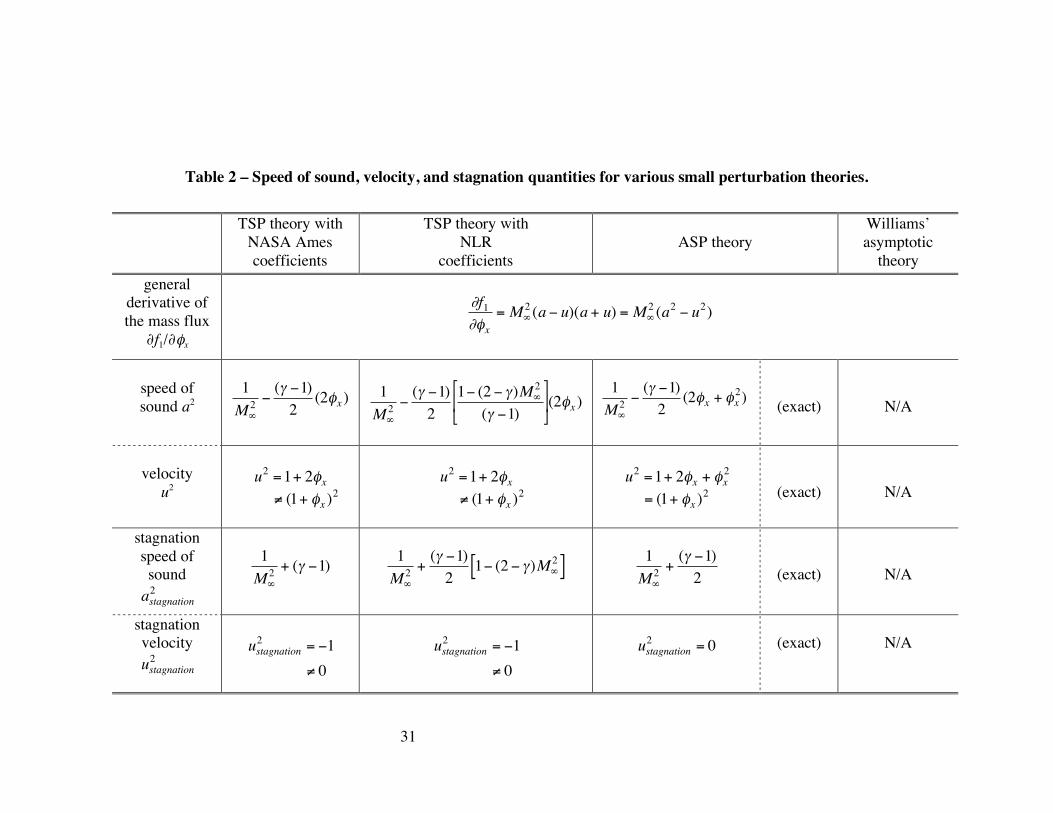
The correct form for the derivative of the mass flux is a symmetric function about u = 0 (stagnation), as shown by the ASP curve in Figure 1(b). This is because the derivative should be positive for subsonic flow, corresponding to u < a, which includes reverse subsonic flow, and the derivative should be negative for supersonic flow, corresponding to u > a, including reverse supersonic flow. When the derivative of the mass flux is positive, the governing equation is of elliptic type, correctly describing subsonic flow. When the derivative is negative, the governing equation is hyperbolic, physically corresponding to supersonic flow. For the ASP theory this is true, independent of the direction of the flow. The other theories not only have the wrong form but they are inaccurate near stagnation and inaccurate for stronger supersonic flows. In fact the worst formulation in this regard is the William’s flux, which explains why applications of CAP-TSD using the William’s flux (default formulation) encounter convergence difficulties, especially on finer meshes. The formulas for the speed of sound, velocity, and stagnation quantities, derived from the derivatives of the mass flux for the various small perturbation theories, are included in Table 2. The entries for Williams’ theory are marked “not available” because the quantities cannot be derived easily from the asymptotic mass flux. All of the quantities tabulated for the ASP theory are exact because the derivative of the mass flux ∂f1/∂φx is exact. Hence, applications of the ASP theory are expected to be accurate for conditions ranging from stagnation to sonic to strong supersonic, including any reverse flow that might occur.
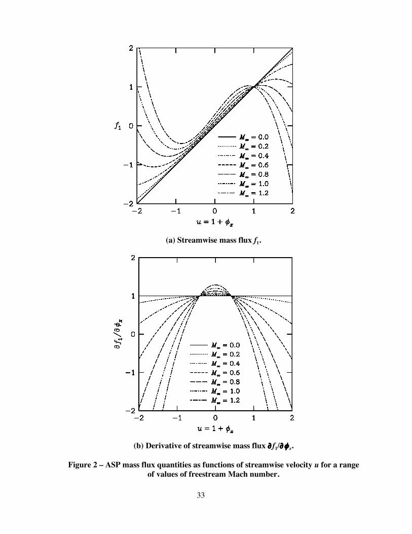
Figure 2 shows flux quantities as functions of streamwise velocity (u = 1 + φx) for the ASP theory computed for freestream Mach numbers ranging from M∞ = 0.0 to 1.2.
7
Figure 2(a) shows the streamwise mass flux f1 and Figure 2(b) shows the derivative of the streamwise mass flux ∂f1/∂φx. Figure 2(a) emphasizes that the ASP mass flux is an asymmetric function about u = 0 (stagnation) and the M∞ = 0.0 result is a line with a slope of unity. If desired the positive offset in f1 can be removed by replacing the constant C = 1 in the ASP mass flux by the constant C = D – E + F, although this modification was not investigated. Of course the derivative is independent of the constant C. Figure 2(b) emphasizes that the derivative of the ASP flux is a symmetric function about u = 0 (stagnation) at any freestream Mach number.
Figure 3 shows an expanded view of the derivative of the mass flux as a function of the streamwise velocity for the M∞ = 0.72 case of Figure 1 to illustrate the differences in sonic points predicted by the various small perturbation formulations. The sonic point is the velocity by which ∂f1/∂φx = 0. As discussed before, the ASP and Williams’ flux formulations possess the exact sonic point by design as shown in Figure 3. The TSP theories with the NLR and NASA Ames coefficients predict values of the sonic velocity that are too high, with the highest value of the sonic velocity corresponding to the NASA Ames formulation. The TSP theory with the NASA Ames coefficients will consequently produce transonic solutions with the smallest supersonic zones and weakest shock waves in comparison with the other formulations. This is due to the flow remaining subsonic until the local velocity exceeds the higher predicted value of the sonic velocity. The TSP theory with the NLR coefficients will generally produce transonic solutions with larger supersonic regions and stronger shocks in comparison with the TSP-NASA Ames theory, but the shock waves will not be as strong as those predicted correctly by either the ASP or Williams’ formulations.
Flow calculations were performed with the small perturbation theories using a 257 x 129 Cartesian finite volume mesh that had a fifty chord extent as shown in Figure 4. The spacing at the leading and trailing edges is Δx = 0.005c, as shown in Figures 5(a) and 5(b), respectively, which is generally considered small for transonic small perturbation applications. All of the solutions were converged at least seven orders of magnitude in the reduction of the L2-norm of the residual. The effects of the streamwise flux on the pressure coefficient distribution for a typical transonic case are shown in Figure 6 for the ASP theory and the TSP theories with the NLR and NASA Ames coefficients. Results were not obtained using Williams’ asymptotic flux because of numerical difficulties in the leading edge region that inhibited convergence. The case considered is that of the NACA 64A410 airfoil at an angle of attack of α = 0° and M∞ = 0.72, the same freestream Mach number used in Figures 1 and 3. As shown in Figure 6, the solution obtained using the TSP theory with the NASA Ames coefficients indicates that there is a smaller supersonic region and a weaker shock wave on the upper surface of the airfoil in comparison with the other two solutions as predicted by the theoretical analysis discussed earlier. The solution obtained using the TSP theory with the NLR coefficients has a slightly stronger shock wave, but the strongest shock wave is predicted by the ASP theory, also consistent with the theoretical analysis. The ASP pressure distribution is in very good agreement with a conservative full-potential (FP) calculation shown in Figure 7, reported by Jameson24 for this case. A comparison of the ASP (Figure 6) and FP (Figure 7) pressure distributions demonstrates that the strength and position of the shock
8
wave near approximately 63% chord on the upper surface of the airfoil are predicted accurately by the ASP formulation. Hence, the ASP mass flux is an essential element in obtaining FP-like solutions with a small perturbation formulation. - Inviscid Irrotational Surface Boundary Conditions
The CAP-TSD code and other small perturbation codes typically use the lowest order
classical small disturbance boundary condition to impose surface tangency given by
!
"z = bx #$ where
!
b(x) " x# = 0 represents the surface. With this boundary condition the velocity and mass flux vectors do not generally coincide, and neither vector is tangent to the surface.
Use of this boundary condition generally results in shock waves that are too weak and located forward in comparison with full potential results. Furthermore such solutions can be shown to be dependent on the local mesh density. Specifically, if the mesh is changed, such as using a finer or coarser mesh, the shock strength and location will be materially changed.
Requiring that the velocity vector be tangent to the surface results in
!
"z = (1+ "x )(bx #$) which may be referred to as a “full potential” surface boundary condition, similar to what is imposed in full potential codes albeit on a body-fitted mesh. However this boundary condition is not consistent with the governing equation and generally leads to solutions involving shock waves that are too strong and located too far aft.
Requiring that the mass flux be tangent to the surface results in
!
"z = f1(bx #$) where f1 is the streamwise mass flux. This boundary condition is consistent with the governing equation (mass consistent) and its use produces solutions that are relatively mesh independent, meaning that the local mesh density does not appreciably affect the shock strength and location.
The ASP capability uses a higher-order mass conserving boundary condition to impose surface tangency given by
!
"z =f1
gbx #$( )
where
9
!
g =1+ H"x +H
2"x2 and
!
H = "(# "1)M$2
Note that
!
g = M"2a2 . This boundary condition was found to be more accurate than the
simpler one above, although the inclusion of the complete vertical flux g in the governing equation had a negligible effect on the solution.
The effects of surface boundary condition (BC) on pressure coefficient distribution are shown in Figure 8 for three forms of the surface BC including the lowest order form used in CAP-TSD labeled “slopes”, the full potential BC where the slopes are scaled by the streamwise velocity (u = 1 + φx), and the mass consistent BC used in the ASP formulation. The calculations were performed for the same NACA 64A410 case presented in Figure 6 and the ASP streamwise flux was used throughout. Figure 8 shows that the use of the lowest order “slopes” BC produces a solution that has a shock wave that is too weak located forward of the correct position. Although not shown here, solutions obtained with the lowest order BC tend to be mesh-dependent because the BC is not mass conserving. Use of the FP BC produces a shock wave that is too strong and located too far aft. In contrast, the mass consistent BC (with the ASP mass flux) leads to the correct shock strength and location, as compared with the Jameson24 FP solution of Figure 9 (same as Figure 7; repeated for direct comparison). Hence, the mass consistent surface boundary condition is an essential element in obtaining FP-like solutions with a small perturbation formulation. - Inviscid Irrotational Wake Boundary Condition
The wake is modeled in all of the small perturbation theories as a planar shear layer
emanating from the trailing edge of the wing. The circulation in the wake is first computed at the trailing edge by
!
"trailingedge
= #$trailingedge
= $upper %$lower
From this starting value the circulation is convected along grid lines downstream of the trailing edge by
!
"t+ "
x= 0
The circulation is incorporated within the solution algorithm using the boundary condition
!
"#z
= 0
which is imposed numerically using
!
"z( )upper
="k # "k#1 + $( )
zk # zk#1 and
!
"z( )lower
="k #$( ) #"k#1zk # zk#1
10
To further demonstrate the accuracy of the ASP capability in producing solutions of similar accuracy to full potential solutions, two additional cases are presented for the NACA 0012 airfoil. The first case is a transonic application of the NACA 0012 airfoil at M∞ = 0.7 and α = 2°. The ASP pressure coefficient distribution is presented in Figure 10 and two full potential solutions for this case reported by Wedan and South25 are presented in Figure 11. Comparisons of the two figures indicate that the strength and location of the shock wave near 28% chord on the upper surface of the airfoil in the ASP result are in very good agreement with the FP results. Also, the ASP pressure distribution near the leading edge where stagnation occurs is smooth and well predicted in comparison with the FP pressure distributions.
The second case is a high lift application of the NACA 0012 airfoil at M∞ = 0.3 and α = 10°. This case is generally regarded as being outside the range of applicability of small perturbation theory, and it is impossible computationally to obtain a converged solution with most small perturbation codes. The ASP pressure coefficient distribution is presented in Figure 12 and two full potential solutions reported by Wedan and South25 are presented in Figure 13. Near the leading edge there is a rapid flow expansion about the upper surface and a small amount of reverse flow (u < 0) on the lower surface due to the relatively high angle of attack. The rapid expansion of the flow produces pressure coefficients close to the value of the sonic pressure coefficient near
!
CP" #7 . The ASP
pressure distribution is in very good agreement with the FP pressure distributions overall, including the prediction of the relatively large values of the pressure coefficients on the upper surface near the leading edge.
- Second-Order Accurate Supersonic Differencing
Most small perturbation codes use first-order accurate differencing at supersonic
points because of difficulty in constructing backward-biased second-order accurate difference stencils. The CAP-TSD code has an option for second-order accurate supersonic differencing but it does not work correctly because of a conceptual error in implementation. Therefore the first-order accurate differencing is used typically and shock waves are generally captured that are slightly weaker and located forward of their correct strength and location. In the ASP capability, a second-order accurate backward (upwind) calculation of the mass flux is achieved at cell interfaces for supersonic points. Similar to reconstruction of flow variables in advanced Euler and Navier-Stokes codes involving Riemann solvers, a flux limiter is required at the shock wave to prevent overshoots or oscillations in the solution because of the change in the solution there. Across the shock wave, although the potential φ is continuous, the velocity u is discontinuous. The flux limiter allows the solution to be second-order accurate in smooth regions, and near the shock wave, the solution is formally first-order accurate.
The effects of order of accuracy of supersonic differencing are demonstrated in Figure 14 for a case involving a strong shock wave. The case considered is a transonic application of the NACA 0012 airfoil at M∞ = 0.75 and α = 2°. Two sets of pressure coefficient distributions are presented corresponding to ASP calculations performed with first- and second-order accurate supersonic differencing. The two sets of pressures are in
11
very close agreement with each other with the only differences in the region of the shock wave on the upper surface of the airfoil. The strong shock in the first-order accurate solution is located near approximately 57% chord and the shock in the second-order solution is of similar strength and located near 60% chord. Figure 15 shows a full potential pressure distribution computed by Hafez26 for this case using an accurate flux-biased method on a reasonably fine mesh. The FP distribution indicates that the strong shock wave is located correctly at approximately 60% chord on the upper surface of the airfoil. Thus, the ASP solution with second-order accurate supersonic differencing accurately predicts the shock location as well as the shock strength. - Entropy and Vorticity Effects
Shock-generated entropy effects are incorporated within small perturbation codes
such as CAP-TSD by first using the Prandtl relation17 (shock jump condition) to determine the velocity downstream of the shock wave from the upstream and sonic velocities. The upstream and downstream velocities are then used in the Rankine-Hugoniot (R-H) relation17 to determine the change in entropy across the shock wave.27 The resulting change in entropy is subsequently used in a Clebsch formulation28 to determine the vorticity downstream of the shock wave.29,30 The vorticity modifies the calculation of the velocity field in the downstream region. This is a common procedure that has been used in various computer codes especially at the full-potential equation level. However, the approach as applied to the small perturbation equation, with any of the fluxes defined above including that of Williams, does not conserve mass.
In contrast, the approach developed for the ASP capability conserves mass by using a ratio of the streamwise fluxes evaluated using the upstream and downstream velocities. Specifically, the downstream perturbation velocity is first computed using the Prandtl relation (shock jump relation) given by
!
"x( )2
=1+ "
x( )sonic
[ ]2
1+ "x( )1
#1
where the subscripts 1 and 2 represent stations that are upstream and downstream of the shock wave, respectively. The change in entropy across the shock is then computed using
!
"s = (# $1) 1$ f1 %x( )1[ ] f1 %x( )
2[ ]{ } For steady flows the entropy is held constant along gridlines downstream of shock waves. For unsteady flows the entropy is convected downstream using
!
"
"t#s+
"
"x#s = 0
The fluxes downstream of the shock are subsequently modified according to
12
!
f1( )nonisentropic
= 1"#s
($ "1)
%
& '
(
) * f1( )
isentropic
which conserves mass across the shock wave by design.
Similar to the CAP-TSD code, the ASP capability uses a Clebsch formulation28 to compute the shock-generated vorticity. In brief, the streamwise velocities downstream of shocks are computed using
!
"x( )rotational
= "x( )irrotational
#$s
%(% #1)M&2
In the CAP-TSD code, when entropy and vorticity effects are included in the
solution procedure no changes are made to the wake modeling because the first order term due to vorticity exactly cancels the first-order entropy term.15 However, the second- order terms were found to be not insignificant, and thus, they were incorporated into the ASP solution procedure. Hence when entropy and vorticity are included, the circulation is convected using
!
"t + "x =(# $1)M%
2 +1
#(# +1)M%2
&s( ) 'x( )[ ]upper
$ &s( ) 'x( )[ ]lower{ }
!
"1
21"
#s( )upper
($ "1)
%
& ' '
(
) * * 1"M+
2( ) ,x2( )upper
!
+1
21"
#s( )lower
($ "1)
%
& '
(
) * 1"M+
2( ) ,x2( )lower
where the subscripts “upper” and “lower” correspond to the values on the upper and lower surfaces of the trailing wake.
The effects of entropy and vorticity modeling are demonstrated in Figure 16. The case considered is the NACA 0012 airfoil at M∞ = 0.75 and α = 2°, the same case presented in Figures 14 and 15. Here, three sets of ASP calculations were performed with the second-order accurate supersonic differencing including: (1) the isentropic capability (the same result shown in Figure 14 with the shock wave located at 60% chord), (2) the Rankine-Hugoniot shock jump relation to calculate the entropy change across the shock, and (3) the mass conserving calculation of the entropy change. When the R-H relation is used to calculate the entropy change the shock wave is weakened and located forward of the isentropic solution. However, when compared to the Euler calculation performed by Hafez26 for this case shown in Figure 17, the R-H shock wave is not located far enough forward on the upper surface of the airfoil. Alternatively when the mass conserving calculation was used to determine the entropy change, a weaker shock
13
located near 46% chord was predicted, which is in very good agreement with the Euler result. Hence, the mass conserving calculation of the entropy change across the shock wave and the inclusion of the second-order terms in the trailing wake are essential elements in producing Euler-like accuracy with the ASP formulation.
To further demonstrate the accuracy of the ASP capability in producing solutions of similar accuracy to Euler solutions, two additional cases are presented for the NACA 0012 airfoil. The first case is a transonic application of the NACA 0012 airfoil at M∞ = 0.6 and α = 5°. This is a difficult case for a small perturbation method because of the higher angle of attack. The ASP pressure coefficient distribution is presented in Figure 18 and several solutions for this case reported by Klopfer and Nixon31 are presented in Figure 19. The latter solutions include calculations involving FP, modified-FP, and Euler codes, the last of which is most relevant. Comparisons of the two figures indicate that the strength and location of the shock wave near 16% chord on the upper surface of the airfoil in the ASP result are in very good agreement with the Euler result. Also, the ASP pressure levels forward of the shock wave are well predicted in comparison with the Euler calculation.
The second case is another transonic application of the NACA 0012 airfoil, this time at M∞ = 0.8 and α = 1.25°. The ASP pressure coefficient distribution is presented in Figure 20 and an Euler solution computed by Anderson, et al.32 with the CFL3D code is presented in Figure 21. The case involves a strong shock wave on the upper surface of the airfoil at approximately 64% chord and a weak shock wave on the lower surface near 34% chord. The difficulty of this case involves the difference in strength of the two shock waves. Comparisons of the two pressure distributions indicate that the ASP formulation including entropy and vorticity accurately predicts the strength and location of both of the shock waves, even though the shocks have disparate strengths. - Viscous Effects
The dissipation integral method developed by Whitfield and coworkers18,19 was
implemented within the ASP3D code to model attached or shock-induced separated boundary layers. The dissipation integral approach represents a significant improvement over the Green’s lag entrainment method such as that in CAP-TSD21 because the closure relations are derived by a detailed fitting of velocity profiles obtained through experiments for both attached and separated flows. Hence, the closure relations are continuous functions applicable to either attached or separated flows, and there is no need for any nonphysical interpolation between disparate sets of closure relations as done by Edwards.21 Drela20 has refined the dissipation integral method, wherein the closure relations depend not only upon the local Mach number and shape factor, but also on the momentum thickness Reynolds number.
The ASP viscous method involves solving the unsteady boundary layer equations simultaneously with the outer potential flow solution so that no interaction law coupling the inner and outer solutions is required. The combined solution procedure involves an implicit block tridiagonal inversion for all of the cells along the surface and trailing wake.
14
Unlike the CAP-TSD viscous capability,21 the ASP capability uses exact formulas for edge quantities and exact boundary conditions are used along surfaces and wakes. Smoothing of edge quantities and limiters are not required for stability, and no arbitrary or free parameters are necessary to tune the procedure.
Specifically in the ASP capability, the exact edge quantities are used for the calculation of velocity ue, density ρe, temperature Te, local Mach number Me, and the coefficient of viscosity µe given by
!
ue
=1+ "x
!
"e
= 1#$ #1
2M%22&
x+ &
x
2( )'
( ) *
+ ,
1
$ #1
!
Te
= 1"# "1
2M$22%
x+ %
x
2( )&
' ( )
* +
!
Me
=M" 1+ #
x( )
1$% $1
2M"22#
x+ #
x
2( )&
' ( )
* +
1 2
!
µe
= Te( )3 2 1+ S T"( )
Te( ) + S T"( )
where S is Sutherland’s coefficient and T∞ is the freestream temperature. These equations are in contrast with the edge quantities contained within CAP-TSD wherein the density, temperature, and local Mach number relations were linearized as
!
"e
=1#M$2%
x
!
Te
=1" # "1( )M$2%
x
!
Me
= M" 1+ 1+# $1
2M"2
%
& '
(
) * +x
,
- .
/
0 1
For the ASP capability, the time-dependent integral boundary layer (IBL) and lag
equations may be written as a system of equations in the form
!
A[ ]"
"t
#
Hk
c$1 2
%
& '
( '
)
* '
+ '
+ B[ ]"
"x
#
Hk
c$1 2
%
& '
( '
)
* '
+ '
+ C[ ],xx
,xt
,tt
%
& '
( '
)
* '
+ '
+ S{ } = 0{ }
15
where the independent variables are the momentum thickness θ, the incompressible shape parameter Hk, and the square root of the shear stress coefficient cτ. The matrix [B] has three eigenvalues that indicate the nature of the boundary layer. For attached boundary layers (Hk < H0) all three eigenvalues are positive, as shown in Figure 22, indicating that all of the characteristics are in the downstream or positive direction. The shape parameter H0 is defined as20
!
H0
= 3+ 400 /Re" if
!
Re" > 400
!
H0
= 4 if
!
Re" # 400 At separation (Hk = H0) one of the eigenvalues becomes zero. And for separated flows (Hk > H0), one of the eigenvalues becomes negative, mathematically reflecting the fact that within the boundary layer there is some reverse flow (in the negative streamwise direction).
For solution, the integral boundary layer and lag equations are first premultiplied by [A]-1 to diagonalize the time term as
!
"
"t
#
Hk
c$1 2
%
& '
( '
)
* '
+ '
+ D[ ]"
"x
#
Hk
c$1 2
%
& '
( '
)
* '
+ '
+ E[ ],xx
,xt
,tt
%
& '
( '
)
* '
+ '
+ F{ } = 0{ }
The resulting IBL system is then linearized in a simple way and cast into the so-called delta-form for implicit solution as
!
"x
"#
"Hk
"c$1 2
%
& '
( '
)
* '
+ '
+ "t G[ ]"#
"Hk
"c$1 2
%
& '
( '
)
* '
+ '
= ,"x"t R{ }
where the viscous residual is defined as
!
R{ } = D[ ]"
"x
#
Hk
c$1 2
%
& '
( '
)
* '
+ '
+ E[ ],xx
,xt
,tt
%
& '
( '
)
* '
+ '
+ F{ }
The system of equations is directly coupled with the ASP equation for the outer
potential flow for simultaneous implicit solution using a block tridiagonal matrix inversion procedure. This is done for the cells adjacent to the upper and lower sides of the lifting surfaces and their wakes. All other cells do not involve the boundary layer, and hence, only the ASP equation is solved in those cells. Dissipation integral relations are used for turbulent closure, similar to those reported by Drela.20
where
!
Re" =#eue"
µe
Re
16
- Surface Boundary Condition Including Entropy, Vorticity, and Viscous Effects
In CAP-TSD the lowest order linear surface tangency condition is used including
entropy, vorticity, and viscous effects. In ASP3D the complete mass-consistent surface boundary condition including entropy, vorticity, and viscous effects is given by
!
"z =f1
gbx #$( ) ±
1
gf1%&( )
x+ bt + %t
*
where
!
f1
= C + D "x( )rotational
+ E "x2( )rotational
+ F "x3( )rotational
and
!
g =1+ H "x( )rotational
+H
2"x2( )rotational
The surface is represented by
!
b(x, t) ± "#(x, t) $ x% = 0
where the ± is for the upper and lower surfaces, respectively, since the boundary layer displacement thickness δ* is defined as a positive quantity on both surfaces. - Wake Boundary Condition Including Entropy, Vorticity, and Viscous Effects
Viscous effects are included in the wake modeling in the ASP capability through the
boundary condition
!
"#z = ±1
gf1$%( )
x+ $t
%
across the wake where f1 and g were defined previously. The boundary condition is incorporated numerically using
!
"z( )upper
="k # "k#1 + $( )
zk # zk#1+1
2
1
gf1%&( )
x+ %t
&'
( )
*
+ ,
and
!
"z( )lower
="k #$( ) #"k#1zk # zk#1
#1
2
1
gf1%&( )
x+ %t
&'
( )
*
+ ,
Three cases were considered to demonstrate the ASP viscous capability
corresponding to an attached boundary layer, a shock-induced flow separation, and a naturally unsteady flow where the boundary layer periodically separates and reattaches. The attached flow case33 is the RAE 2822 airfoil at M∞ = 0.676, α = -2.25°, and Re = 5.7 x 10⁶, where the calculations were performed using a CFL number of thirty for five hundred time steps, and the results are presented in Figure 23. Figure 23(a) shows the convergence histories of the residuals for the outer potential flow Rφ and the inner IBL
17
equations Rθ,
!
RH
k
and
!
Rc"
on the upper surface of the airfoil. The residuals indicate that the solutions for both the outer ASP potential flow and the inner IBL indeed converge. The corresponding ASP pressure coefficient distribution is compared with the experimental pressure data33 in Figure 23(b). These comparisons show very good agreement between the ASP pressures and the data, thus demonstrating the accuracy of the ASP viscous capability.
The second case34 corresponds to separated flow on the upper surface of the NACA 0012 airfoil at M∞ = 0.775, α = 2.05°, and Re = 107. The calculations were performed with a CFL number of fifteen for a total of one thousand time steps and the results are presented in Figure 24. The CFL number for the separated flow case was half of that used in the attached flow case, although it is still a relatively large value. Figure 24(a) shows the convergence history in the more conventional form of the residual of the ASP potential equation. The convergence history indicates that the solution has converged approximately five orders of magnitude for the separated flow case. The corresponding ASP pressure coefficient distribution is shown in Figure 24(b), which is in good agreement with the experimental data,34 especially in the strength and location of the upper surface shock wave. The shock induced separation along the upper surface of the airfoil ranges from the foot of the shock near 53% chord to the reattachment point at approximately 67% chord.
The third case33 that was considered to demonstrate the ASP viscous capability was the periodic flow separation about the RAE 2822 airfoil at M∞ = 0.75, α = 2.81°, and Re = 6.5 x 10⁶. The calculations were performed using a CFL number of twenty and the resulting lift and moment coefficient time histories are shown in Figure 25(a) for a total of three thousand time steps. The calculations were run much longer than the previous two cases to demonstrate clearly the periodicity of the coefficients as a function of time. In this case the flow on the upper surface of the airfoil periodically separates and later reattaches through each of the cycles shown. The instantaneous ASP pressure coefficient distribution at t = 3000Δt is shown in Figure 24(b). The pressure distribution is smooth near the shock and the trailing edge, which are the two regions of strongest interaction between the boundary layer and the outer potential flow. Although not obvious from the figure, the flow is separated from the shock wave near 64% chord to the trailing edge.
Introduction of the ASP3D Computer Program
The ASP theory has been used as the basis for a new computer code called ASP3D
(Advanced Small Perturbation – 3D), which involves either AF1- or AF2-type approximate factorization algorithms and a FAS (full approximation scheme) multigrid procedure for the solution of the ASP potential flow equation and associated boundary conditions. The ASP3D code can treat aircraft configurations involving multiple lifting surfaces with leading and trailing edge control surfaces and a fuselage. The new code is briefly described here and some representative results are presented in the following section.
18
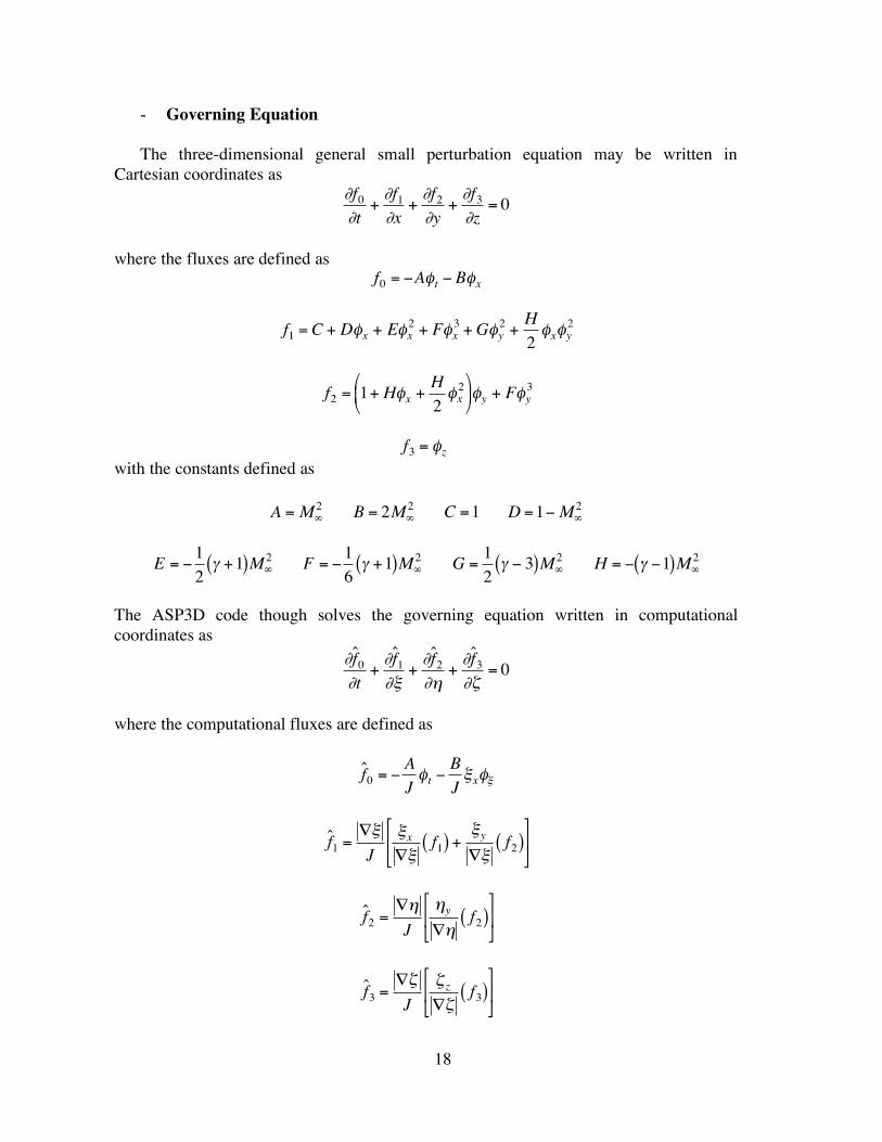
- Governing Equation
The three-dimensional general small perturbation equation may be written in Cartesian coordinates as
!
"f0
"t+"f1
"x+"f2
"y+"f3
"z= 0
where the fluxes are defined as
!
f0
= "A#t " B#x
!
f1
= C + D"x + E"x2
+ F"x3
+G"y2
+H
2"x"y
2
!
f2
= 1+ H"x +H
2"x2
#
$ %
&
' ( "y + F"y
3
!
f3
= "z with the constants defined as
!
A = M"2
!
B = 2M"2
!
C =1
!
D =1"M#2
!
E = "1
2# +1( )M$
2
!
F = "1
6# +1( )M$
2
!
G =1
2" # 3( )M$
2
!
H = " # "1( )M$2
The ASP3D code though solves the governing equation written in computational coordinates as
!
"ˆ f 0
"t+"ˆ f
1
"#+"ˆ f
2
"$+"ˆ f
3
"%= 0
where the computational fluxes are defined as
!
ˆ f 0
= "A
J#t "
B
J$x#$
!
ˆ f 1
="#
J
#x
"#f1( ) +
#y
"#f
2( )$
% &
'
( )
!
ˆ f 2
="#
J
#y
"#f
2( )$
% &
'
( )
!
ˆ f 3
="#
J
# z
"#f
3( )$
% &
'
( )
19
The various geometric quantities used in these equations such as the cell volume, areas of the cell interfaces, and direction cosines are defined elsewhere.22 All of these quantities are computed using formulas that are exact. - Entropy, Vorticity, and Viscous Effects
Shock-generated entropy and vorticity effects are incorporated within the ASP3D
code using the mass consistent modeling as described earlier. Viscous effects are included through a simultaneous implicit solution of the integral boundary layer and lag equations with the outer ASP potential flow as also described earlier. The ASP3D capability does not require the use of an interaction law because the equations are solved simultaneously. This is a stable approach that also does not require any smoothing or limiters. Turbulent closure is through the use of the dissipation integral relations of Drela,20 which is applicable to attached and separated flows. - Surface Boundary Condition
In CAP-TSD the lowest order linear surface tangency condition is used including
entropy, vorticity, and viscous effects. In ASP3D the complete mass-consistent surface boundary condition including entropy, vorticity, and viscous effects is given by
!
"z =f
gbx #$( ) + "yby ±
1
gf%&( )
x+ bt + %t
*
where
!
f = C + D "x( )rotational
+ E "x2( )rotational
+ F "x3( )rotational
!
"A#y2 +
H
2#y2 #x( )
rotational
and
!
g =1+ H "x( )rotational
+H
2"x2( )rotational
+H
2"y2( )
The surface is represented by
!
b(x,y,t) ± "#(x,t) $ x% = 0
where the ± is for the upper and lower surfaces, respectively, since the boundary layer displacement thickness δ* is defined as a positive quantity on both surfaces.
Note that the spanwise slopes by are included in the complete surface boundary condition for three-dimensional applications, which may be important for swept wings near the leading edge and also in the wing tip region. Furthermore, the streamwise and spanwise slopes are computed internal to ASP3D from the ordinates of the wing geometry by simple second-order accurate central finite differences, effectively the same as is done in advanced codes with body fitted meshes. This eliminates the differentiation of the spline of the wing geometry normally performed as a preprocessing step to
20
determine the airfoil slopes. It thus makes the input to the ASP3D code simpler than most other small perturbation codes such as CAP-TSD.
- Wake Boundary Condition
Viscous effects are included in the wake modeling in the ASP capability through the
boundary condition
!
"#z = ±1
gf$%( )
x+ $t
%
across the wake where f and g were defined previously. The boundary condition is incorporated numerically using
!
"z( )upper
="k # "k#1 + $( )
zk # zk#1+1
2
1
gf%&( )
x+ %t
&'
( )
*
+ ,
and
!
"z( )lower
="k #$( ) #"k#1zk # zk#1
#1
2
1
gf%&( )
x+ %t
&'
( )
*
+ ,
- Shock Capturing
The AF1 and AF2 algorithms of the ASP3D code use one of three approaches to
model supersonic regions of the flow including: 1) Godunov,35 2) Engquist-Osher36 (E-O), and 3) Murman-Cole37 (M-C) type-dependent switches. The first two switches satisfy an entropy inequality by design. This means that their use precludes the possibility of computing nonphysical expansion shocks that can occur with the Murman-Cole switch, especially in two-dimensional applications. With Godunov35 switching, shocks are captured sharply, with only one interior state. Therefore, the Godunov switch is preferable over the E-O and M-C switches, and it is the default switch within the ASP3D code. The E-O switch is available for comparisons with CAP-TSD, and the M-C switch was included for completeness and historical reasons. The details of the ASP3D implementation of the shock capturing options are reported by Batina.22 - Solution Algorithm
The ASP3D code involves a modern cell-centered finite-volume discretization, which
allows exact planform treatment including leading edges, wing tips, and control surface edges. The advanced small perturbation equation is solved using either an AF1 approximate factorization algorithm or an AF2-type algorithm. The AF1 algorithm within the ASP3D code is the cell-centered finite-volume version of the AF1 algorithm13 developed for CAP-TSD, which may be written as
!
L" L#L$%& = 'R &( )
21
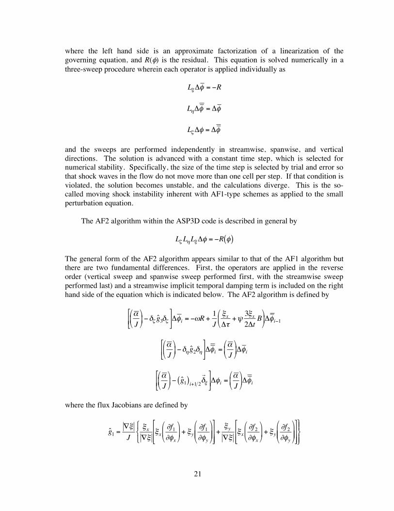
where the left hand side is an approximate factorization of a linearization of the governing equation, and R(φ) is the residual. This equation is solved numerically in a three-sweep procedure wherein each operator is applied individually as
!
L"#$ = %R
!
L"#$ = #$
!
L"#$ = #$ and the sweeps are performed independently in streamwise, spanwise, and vertical directions. The solution is advanced with a constant time step, which is selected for numerical stability. Specifically, the size of the time step is selected by trial and error so that shock waves in the flow do not move more than one cell per step. If that condition is violated, the solution becomes unstable, and the calculations diverge. This is the so-called moving shock instability inherent with AF1-type schemes as applied to the small perturbation equation.
The AF2 algorithm within the ASP3D code is described in general by
!
L" L#L$%& = 'R &( ) The general form of the AF2 algorithm appears similar to that of the AF1 algorithm but there are two fundamental differences. First, the operators are applied in the reverse order (vertical sweep and spanwise sweep performed first, with the streamwise sweep performed last) and a streamwise implicit temporal damping term is included on the right hand side of the equation which is indicated below. The AF2 algorithm is defined by
!
"
J
#
$ %
&
' ( )*+ ˆ g
3*+
,
- .
/
0 1 23 i = )4R +
1
J
5x
26+7
35x
22tB
#
$ %
&
' ( 23 i)1
!
"
J
#
$ %
&
' ( )*+ ˆ g
2*+
,
- .
/
0 1 23 i =
"
J
#
$ %
&
' ( 23 i
!
"
J
#
$ %
&
' ( ) ˆ g
1( )i+1 2
r * +
,
- .
/
0 1 23i =
"
J
#
$ %
&
' ( 23 i
where the flux Jacobians are defined by
!
ˆ g 1
="#
J
#x
"#
$ % &
#x
'f1
'(x
)
* +
,
- . + #y
'f1
'(y
)
* + +
,
- . .
/
0 1 1
2
3 4 4
!
+"y#"
"x$f2
$%x
&
' (
)
* + + "y
$f2
$%y
&
' ( (
)
* + +
,
- . .
/
0 1 1
2
3 4
5 4
22
!
ˆ g 2
="#
J
#y
"##y
$f2
$%y
&
' ( (
)
* + +
,
- . .
/
0 1 1
2
3 4
5 4
6
7 4
8 4
!
ˆ g 3
="#
J
# z
"## z
$ % &
' ( )
In the first sweep, the temporal damping term is treated implicitly since it involves information from the second intermediate sweep but at the previous grid plane i - 1, and
!
" =#x
$%+&
2
$t2A +
3#x
2$tB
'
( )
*
+ ,
The parameter ψ is set equal to zero for steady applications and set equal to unity for unsteady applications. The parameter ω is an over-relaxation factor. The algorithm involves both physical (Δt) and computational (Δτ) time steps. The computational step is selected for rapid convergence and it is usually assigned a large value. Hence the solution can be advanced using either a constant computational time step or a constant CFL number. The physical time step is used only for unsteady applications, and it is selected based on the physics of the problem being considered.
The AF2 approach is the preferred algorithm. The AF2 scheme is more robust than the AF1 scheme since it cannot fail due to the moving shock instability by design. The temporal damping term eliminates the moving shock instability. Hence convergence to steady state is achieved with large time steps or large CFL numbers, independent of the moving shock instability that plagues the AF1 algorithm. The AF2 scheme may also be used for unsteady calculations when local iteration is applied. Therefore, the physical time step may be selected based on the physics of the problem being solved, rather than on numerical stability considerations. For either steady or unsteady applications, the temporal damping term vanishes in the steady-state limit or within the convergence process of performing subiterations for unsteady calculations. - Multigrid Implementation
The AF1 algorithm is not appropriate for multigrid implementation because the rapid
rate of convergence of the multigrid procedure would result in the moving shock instability. The AF2 algorithm of the ASP3D code is amenable to multigrid implementation because the temporal damping term prevents the moving shock instability from occurring. Therefore the multigrid procedure38 may be used for steady or iterative unsteady applications with ASP3D. The procedure is implemented in FAS (Full Approximation Scheme) form,39 which is applicable to nonlinear governing equations. As with any multigrid procedure, high-frequency errors are damped on the fine mesh and low-frequency errors are damped on the coarser meshes. Either V- or W-cycles may be selected and full multigrid is available. W-cycles have been found to be slightly more
23
effective for solution convergence, although W-cycles are slightly more expensive than V-cycles.40
Specifically, the calculation on the finest mesh (N) smoothes high frequency errors using the AF2 algorithm written in general form
!
LN"N( ) = R
N
Subsequent calculations on the next coarser mesh (N-1) involve fine mesh residual injection
!
LN"1 #N"1( ) = R
N"1 "ˆ I
N
N"1R
N( ) + LN"1IN
N"1 #N( )
where the I functions are restriction operators for transferring the velocity potential and residual from the fine mesh to the coarse mesh. The procedure is generally repeated for additional coarse meshes (N-2, N-3, …).
The restriction operator40 for potential is a volume weighted operator defined by
!
"N#1 = I
N
N#1"N
=$V"
N
$V
and the restriction operator40 for residuals is defined by
!
ˆ I N
N"1R
N=#R
N
where the summations above are taken over all of the fine mesh cells that make up the coarse mesh cell. The interpolation operator for the velocity potential that is required to transfer information back from coarse to fine mesh is a trilinear interpolation operator defined symbolically by
!
"N#"
N+ I
N$1N "
N$1
ASP3D Results and Discussion
Representative ASP3D results are presented briefly to demonstrate application of the ASP theory to more practical problems. Two cases were considered including: (1) inviscid and viscous calculations for the F-5 fighter wing41 and (2) viscous calculations for the NACA RM L51F07 wing-fuselage configuration.42 All of the results are compared with experimental data to assess the accuracy of the ASP3D computations. - F-5 Fighter Wing Results
The F-5 fighter wing41 has a leading edge sweep of 31.92 degrees, an aspect ratio of
1.578, and a taper ratio of 0.283. The wing has a NACA 65A004.8 airfoil section that has a drooped leading edge. The wing was modeled for ASP3D applications using a 97 x
24
25 x 65 finite volume mesh as shown in Figure 26. A near field view of the 97 x 25 planform mesh is shown in Figure 26(a) and a view of the 97 x 65 root sectional mesh is shown in Figure 26(b). The meshes were generated using a program that was created to construct meshes specifically for use by the ASP3D code, and as such, it can generate meshes for aircraft configurations with multiple lifting surfaces, with multiple leading and trailing edge controls, and a fuselage. The mesh generator automatically creates the input file for ASP3D, which makes it user friendly.
Inviscid and viscous calculations were performed both using the entropy and vorticity effects for the F-5 wing at M∞ = 0.946, α = -0.004°, and Re = 5.89 x 10⁶. These results are presented in Figure 27, with the inviscid pressure distributions shown in Figure 27(a) and the viscous pressure distributions shown in Figure 27(b). The ASP3D pressure distributions were interpolated to the eight span stations where the NLR experimental data41 were measured ranging from η = 0.174 in the inboard region of the wing to η = 0.939 near the wing tip. The inviscid pressure distributions (Figure 27(a)) show generally good agreement with the experimental pressure data except in the shock region on the upper and lower surfaces of the wing. This is expected because of the neglect of viscous effects. The viscous pressure distributions (Figure 27(b)) are similar to the inviscid pressures and thus also agree well with the data, although the shock waves are slightly weaker and located more forward, and hence, they are in better agreement with the experimental shock results. - NACA RM L51F07 Wing-Fuselage Results
The geometry of the NACA RM L51F07 wing-fuselage configuration42 is defined in
Figure 28. The wing has a leading edge sweep of 46.76 degrees (quarter chord sweep of 45 degrees), an aspect ratio of 4.0, and a taper ratio of 0.6. The wing has a NACA 65A006 airfoil section. The fuselage is an axisymmetric body with fineness ratio of 12. The model was sting mounted for testing and pressures were measured along five chords of the wing as well as on the fuselage. The NACA RM L51F07 configuration was modeled for ASP3D applications using a 129 x 29 x 75 finite volume mesh. A near field view of the 129 x 29 planform mesh is shown in Figure 29. The mesh was generated in the streamwise direction by clustering points near the wing, and there is a slight clustering near the fuselage nose and where the fuselage is attached to the sting. The mesh was generated in the spanwise direction by clustering cells near the fuselage and near the wing tip.
Viscous calculations were performed using the entropy and vorticity effects for the NACA RM L51F07 configuration at M∞ = 0.93, α = 2.0°, and Re = 107. These results are presented in Figure 30 including comparisons with experiment data,42 with the wing pressure comparisons shown in Figure 30(a) and the fuselage pressure comparisons shown in Figure 30(b). The ASP3D pressure distributions on the wing were interpolated to the five span stations where experimental data42 were measured ranging from η = 0.2 near the wing fuselage junction to η = 0.95 near the wing tip. The ASP3D pressure distributions on the fuselage were directly computed along the fuselage centerline for comparison with the experimental data measured at η = 0.0. The wing pressure
25
comparisons of Figure 30(a) show good overall agreement in pressure levels and in the prediction of the strength and location of the upper surface shock wave. The largest differences between computation and experiment are in the inboard region at η = 0.2, which may be the case because there is no boundary layer on the fuselage (only on the wing). The fuselage pressure comparisons of Figure 30(b) also show good agreement although the calculated shock wave is a little sharper than the wing shock wave due to the neglect of viscous effects on the fuselage.
Conclusions
A new advanced small perturbation (ASP) potential flow theory was developed by first determining the essential elements required to produce solutions as accurate as a full potential code with the small perturbation approach on a Cartesian grid. This level of accuracy was obtained by using a higher-order streamwise mass flux and a mass conserving surface boundary condition. Subsequent applications with these improvements showed very good agreement with all of the full potential cases considered. This was true even for cases at freestream Mach numbers as low as 0.3 and angles of attack as high as ten degrees, conditions that are normally considered to be outside the range of applicability of classical small perturbation theories.
The ASP theory was further developed to produce Euler-like solutions by incorporating a mass conserving calculation of the entropy jump across of the shock wave based on the higher-order streamwise mass flux of the ASP theory. Second-order terms in the trailing wake boundary condition were found to be not insignificant for lifting cases and were also incorporated. Subsequent calculations with these modifications showed very good agreement with all of the Euler cases that were considered. This was true for cases involving strong shock waves and multiple shock waves of disparate strengths.
Viscous effects were incorporated within the ASP formulation by coupling an integral boundary layer procedure to the outer inviscid flow calculation. The dissipation integral method was implemented to model attached or shock-induced separated boundary layers. The capability involves solving the unsteady boundary layer and lag equations simultaneously with the outer potential flow solution, so that no interaction law coupling the inner and outer solutions is required. The combined solution procedure involves an implicit block tridiagonal inversion for all of the cells along the surface and its trailing wake. Exact formulas for edge quantities and exact boundary conditions are used along surfaces and wakes. Smoothing of edge quantities and limiters are not required for stability, and no arbitrary or free parameters are necessary to tune the procedure. Calculations performed with the complete ASP capability including entropy, vorticity, and viscous effects showed good agreement with experimental data.
The ASP theory was shown to be mathematically more appropriate and computationally more accurate than the classical TSP theories. Consequently, the new theory has been used as the basis for a new computer code called ASP3D (Advanced Small Perturbation – 3D), which involves either AF1- or AF2-type approximate
26
factorization algorithms and a FAS (full approximation scheme) multigrid procedure for the solution of the ASP potential flow equation. The ASP3D code can treat aircraft configurations involving multiple lifting surfaces with leading and trailing edge control surfaces and a fuselage. The new code was briefly described and some representative results were presented. Detailed descriptions of the ASP3D capability and comprehensive results and comparisons are reported in a companion publication.22
Acknowledgement
The NASA Langley Research Center supported the work contained herein while the author was employed as a Senior Research Scientist in the Configuration Aerodynamics Branch.
References
1. Edwards, J. W.; and Thomas, J. L.: Computational Methods for Unsteady Transonic Flows, AIAA Paper No. 87-0107, January 1987.
2. Edwards, J. W.; and Malone, J. M.: Current Status of Computational Methods for
Transonic Unsteady Aerodynamics and Aeroelastic Applications, AGARD CP-507, March 1992, pp. 1-1 to 1-24.
3. Schuster, D. M.; Liu, D. D.; and Huttsell, L. J.: Computational Aeroelasticity:
Success, Progress, Challenge, AIAA Paper No. 2003-1725, April 2003. 4. Borland, C. J.; and Rizzetta, D. P.: Nonlinear Transonic Flutter Analysis, AIAA
Journal, Vol. 20, November 1982, pp. 1606-1615. 5. Batina, J. T.; Seidel, D. A.; Bland, S. R.; and Bennett, R. M.: Unsteady Transonic
Flow Calculations for Realistic Aircraft Configurations, AIAA Paper No. 87-0850, April 1987; also Journal of Aircraft, Vol. 26, January 1989, pp. 21-28.
6. Batina, J. T.: Unsteady Euler Algorithm with Unstructured Dynamic Mesh for
Complex-Aircraft Aerodynamic Analysis, AIAA Paper No. 89-1189, April 1989; also AIAA Journal, Vol. 29, No. 3, March 1991, pp. 327-333.
7. Bennett, R. M.; Bland, S. R.; Batina, J. T.; Gibbons, M. D.; and Mabey, D. G.:
Calculation of Steady and Unsteady Pressures on Wings at Supersonic Speeds with a Transonic Small-Disturbance Code, AIAA Paper 87-0851, April 1987.
8. Cunningham, H. J.; Batina, J. T.; and Bennett, R. M.: Modern Wing Flutter
Analysis by Computational Fluid Dynamics Methods, ASME Paper No. 87-WA/Aero-9, December 13-18, 1987; also Journal of Aircraft, Vol. 25, October 1988, pp. 962-968.
27
9. Bennett, R. M.; Batina, J. T.; and Bland, S. R.: Wing-Flutter Calculations with the CAP-TSD Unsteady Transonic Small-Disturbance Program, AIAA Paper No. 88-2347, April 1988; also Journal of Aircraft, Vol. 26, September 1989, pp. 876-882.
10. Gibbons, M. D.: Aeroelastic Calculations using CFD for a Typical Business Jet
Model, NASA CR-4753, September 1996.
11. Gibbons, M. D.: personal communication, October 20, 1994.
12. Steinhoff, J.; and Jameson, A.: Multiple Solutions of the Transonic Potential Flow Equation, AIAA Paper No. 81-1019, June 1981.
13. Batina, J. T.: An Efficient Algorithm for Solution of the Transonic Small-
Disturbance Equation, AIAA Paper No. 87-0109, January 1987; also Journal of Aircraft, Vol. 25, July 1988, pp. 598-605.
14. Batina, J. T.: Unsteady Transonic Algorithm Improvements for Realistic Aircraft
Applications, AIAA Paper No. 88-0105, January 1988; also Journal of Aircraft, Vol. 26, February 1989, pp. 131-139.
15. Batina, J. T.: Unsteady Transonic Small-Disturbance Theory Including Entropy
and Vorticity Effects, AIAA Paper No. 88-2278, April 1988; also Journal of Aircraft, Vol. 26, June 1989, pp. 531-538.
16. Jones, D. J.: Reference Test Cases and Contributors, Test Cases for Inviscid Flow
Field Methods, AGARD-AR-211, May 1985.
17. Kuethe, A. M.; and Chow, C.-Y.: Foundations of Aerodynamics: Bases of Aerodynamic Design, John Wiley and Sons, New York, Third Edition, 1976.
18. Whitfield, D. L.: Analytical Description of the Complete Two-Dimensional
Turbulent Boundary-Layer Velocity Profile, AEDC-TR-77-79, September 1977; also AIAA Paper No. 78-1158, July 1978.
19. Swafford, T. W.: Analytical Approximation of Two-Dimensional Separated
Turbulent Boundary-Layer Velocity Profiles, AEDC-TR-79-99, October 1980.
20. Drela, M.: Two-Dimensional Transonic Aerodynamic Design and Analysis Using the Euler Equations, GTL Report No. 187, February 1986.
21. Edwards, J. W.: Transonic Shock Oscillations Calculated with a New Interactive
Boundary Layer Coupling Method, AIAA Paper No. 93-0777, January 1993.
28
22. Batina, J. T.: Introduction to the ASP3D Computer Program for Transonic Unsteady Aerodynamic and Aeroelastic Analysis, NASA/TM-2005-213909, 2005.
23. Fuglsang, D. F.; and Williams, M. H.: Non-Isentropic Unsteady Transonic Small
Disturbance Theory, AIAA Paper 85-0600, April 1985.
24. Jameson, A.: Transonic Flow Calculations, Lecture Series 87, Computational Fluid Dynamics, von Karman Institute for Fluid Dynamics, March 15-19, 1976.
25. Wedan, B.; and South, J. C.: A Method for Solving the Transonic Full-Potential
Equation for General Configurations, AIAA Paper No. 83-1889, July, 1983.
26. Hafez, M. M.: Numerical Algorithms for Transonic Inviscid Flow Calculations, Advances in Computational Transonics, Volume 4 in the Series, Recent Advances in Numerical Methods in Fluids, Ed. W. G. Habashi, Pineridge Press, Swansea, UK, 1985.
27. Hafez, M.; and Lovell, D.: Entropy and Vorticity Corrections for Transonic
Flows, AIAA Paper No. 83-1926, July 1983.
28. Clebsch, A.: Uber die Integration der Hydrodynamischen Gleichungen, J. Reine Angew. Math., Vol. 57, 1959, pp. 1-10.
29. Grossman, B.: The Computation of Inviscid Rotational Gasdynamic Flows Using
an Alternate Velocity Decomposition, AIAA Paper No. 83-1900, July 1983.
30. Dang, T. Q.; and Chen, L. T.: An Euler Correction Method for Two- and Three-Dimensional Transonic Flows, AIAA Paper No. 87-0522, January 1987.
31. Klopfer, G. H.; and Nixon, D.: Nonisentropic Potential Formulation for
Transonic Flows, AIAA Journal, Vol. 22, No. 6, June 1984, pp. 770-776.
32. Anderson, W. K.; Thomas, J. L.; and van Leer, B.: Comparison of Finite-Volume Flux-Vector Splittings for the Euler Equations, AIAA Paper No. 85-0122, January 1985.
33. Cook, P. H.; McDonald, M. A.; and Firmin, M. C. P.: Aerofoil RAE 2822 –
Pressure Distribution, and Boundary Layer and Wake Measurements, Experimental Data Base for Computer Program Assessment, AGARD-AR-138, May 1979.
34. McDevitt, J. B.; and Okuno, A. F.: Static and Dynamic Pressure Measurements
on a NACA 0012 Airfoil in the Ames High Reynolds Number Facility, NASA TP-2485, June 1985.
29
35. Godunov, S.: A Finite Difference Method for the Numerical Computation of Discontinuous Solutions of the Equations of Fluid Dynamics, Mathematics of the USSR, Sbornik, Vol. 47, 1959.
36. Engquist, B. E.; and Osher, S. J.: Stable and Entropy Satisfying Approximations
for Transonic Flow Calculations, Mathematics of Computation, Vol. 34, No. 149, January 1980, pp. 45-75.
37. Murman, E. M.: Analysis of Embedded Shock Waves Calculated by Relaxation
Methods, Proceeds of the AIAA Computational Fluid Dynamics Conference, July 1973, pp. 27-40.
38. Jameson, A.: Acceleration of Transonic Potential Flow Calculations on Arbitrary
Meshes by the Multiple Grid Method, AIAA Paper No. 79-1458, July 1979.
39. Brandt, A.: Multi-Level Adaptive Solutions to Boundary-Value Problems, Mathematics of Computation, Vol. 31, April 1977, pp. 333-390.
40. Anderson, W. K.: Implicit Multigrid Algorithms for the Three-Dimensional Flux
Split Euler Equations, Doctoral Thesis, Mississippi State University, Mississippi, August 1986.
41. Tijdeman, H.; Van Nunen, J. W. G.; Kraan, A. N.; Persoon, A. J.; Poestkoke, R.;
Roos, R.; Schippers, P.; and Siebert, C. M.: Transonic Wind Tunnel Tests on an Oscillating Wing with External Stores, AFFDL-TR-78-194, December 1978.
42. Loving, D. L.; and Estabrooks, B. B.: Transonic-Wing Investigation in the
Langley 8-Foot High-Speed Tunnel at High Subsonic Mach Numbers and at a Mach Number of 1.2, Analysis of Pressure Distribution of Wing-Fuselage Configuration Having a Wing of 45° Sweepback, Aspect Ratio 4, Taper Ratio 0.6, and NACA 65A006 Airfoil Section, NACA RM L51F07, September 1951.
30
Table 1 - Mass flux, derivative of mass flux, and sonic velocity for various small perturbation theories.
TSP theory with NASA Ames coefficients
TSP theory with NLR
coefficients
ASP theory
Williams’ asymptotic expansion theory
small perturbation mass flux f1
!
f1
= C + D"x + E"x2
+ F"x3
!
f1 = (" +1)M#21+ ($x )sonic[ ] VVsonic %
V2
2
&
' (
)
* +
!
C =1
!
D =1"M#2
!
E = "1
2(# +1)M$
2
!
E = "1
23" (2 " #)M$
2[ ]M$2
!
E = "1
2(# +1)M$
2
associated
coefficients or parameters
!
F = 0
!
F = 0
!
F = "1
6(# +1)M$
2
!
V ="x
1+"x
2 + ("x)sonic
!
Vsonic
=1+ ("
x)sonic[ ]
2#1
2 1+ ("x)sonic[ ]
derivative of the mass flux
∂f1/∂φx
!
"f1
"#x= D+ 2E#x + 3F#x
2
!
"f1"#x
= ($ +1)M%21+ (#x )sonic[ ] Vsonic &V( )
dV
d#x
sonic velocity
usonic = 1 + (φx)sonic
!
1+(1"M#
2)
($ +1)M#2
!
1+(1"M#
2)
3" (2 " $)M#2[ ]M#
2
!
1+2(1"M#
2)
($ +1)M#2
%
& '
(
) *
1/ 2
(exact)
!
1+2(1"M#
2)
($ +1)M#2
%
& '
(
) *
1/ 2
(exact)
31
Table 2 – Speed of sound, velocity, and stagnation quantities for various small perturbation theories.
TSP theory with
NASA Ames coefficients
TSP theory with NLR
coefficients
ASP theory
Williams’ asymptotic
theory general
derivative of the mass flux
∂f1/∂φx
!
"f1"#x
= M$2(a % u)(a + u) = M$
2(a2 % u2)
speed of sound a2
!
1
M"2#($ #1)
2(2%
x)
!
1
M"2#($ #1)
2
1# (2 # $)M"2
($ #1)
%
& '
(
) * (2+x )
!
1
M"2#($ #1)
2(2%
x+ %
x
2)
(exact)
N/A
velocity u2
!
u2
=1+ 2"x
!
" (1+ #x)2
!
u2
=1+ 2"x
!
" (1+ #x)2
!
u2
=1+ 2"x
+ "x
2
!
= (1+ "x)2
(exact)
N/A
stagnation speed of sound
!
astagnation2
!
1
M"2
+ (# $1)
!
1
M"2
+(# $1)
21$ (2 $ #)M"
2[ ]
!
1
M"2
+(# $1)
2
(exact)
N/A
stagnation velocity
!
ustagnation2
!
ustagnation2
= "1
!
" 0
!
ustagnation2
= "1
!
" 0
!
ustagnation2
= 0
(exact)
N/A
32
(a) Streamwise mass flux f1.
(b) Derivative of streamwise mass flux ∂f1/∂φx.
Figure 1 - Mass flux quantities as functions of streamwise velocity u for various
small perturbation theories at M∞ = 0.72.
33
(a) Streamwise mass flux f1.
(b) Derivative of streamwise mass flux ∂f1/∂φx.
Figure 2 – ASP mass flux quantities as functions of streamwise velocity u for a range of values of freestream Mach number.
34
Figure 3 - Sonic point (∂f1/∂φx = 0) as a function of streamwise velocity u for various small perturbation theories at M∞ = 0.72.
35
Figure 4 – Cartesian finite volume mesh (257 x 129) with fifty chord extent for airfoil applications using the various small perturbation theories.
(a) Leading edge region. (b) Trailing edge region.
Figure 5 – Near field views of the finite volume mesh for airfoil applications using the various small perturbation theories.
trailing edge
leading edge
airfoil slit
airfoil slit
36
Figure 6 - Effects of small perturbation streamwise flux on pressure coefficient distribution for the NACA 64A410 airfoil at M∞ = 0.72 and α = 0° .
Figure 7 – Full potential pressure coefficient distribution computed by Jameson24 for the NACA 64A410 airfoil at M∞ = 0.72 and α = 0° .
shock location
37
Figure 8 - Effects of small perturbation surface boundary condition on pressure coefficient distribution for the NACA 64A410 airfoil at M∞ = 0.72 and α = 0° .
Figure 9 – Full potential pressure coefficient distribution computed by Jameson24 for the NACA 64A410 airfoil at M∞ = 0.72 and α = 0° (same as Figure 7).
shock location
38
Figure 10 – ASP pressure coefficient distribution for the NACA 0012 airfoil at
M∞ = 0.7 and α = 2° .
Figure 11 – Full potential pressure coefficient distributions reported by Wedan and South25 for the NACA 0012 airfoil at M∞ = 0.7 and α = 2° .
shock location
39
Figure 12 – ASP pressure coefficient distribution for the NACA 0012 airfoil at M∞ = 0.3 and α = 10° .
Figure 13 – Full potential pressure coefficient distributions reported by Wedan and South25 for the NACA 0012 airfoil at M∞ = 0.3 and α = 10° .
!
Cp"
40
Figure 14 - Effects of order of accuracy of supersonic differencing on pressure coefficient distribution for the NACA 0012 airfoil at M∞ = 0.75 and α = 2°.
Figure 15 – Full potential pressure coefficient distribution computed by Hafez26 for the NACA 0012 airfoil at M∞ = 0.75 and α = 2° .
shock location
41
Figure 16 - Effects of small perturbation entropy and vorticity modeling on pressure coefficient distribution for the NACA 0012 airfoil at M∞ = 0.75 and α = 2°.
Figure 17 – Euler pressure coefficient distribution computed by Hafez26 for the NACA 0012 airfoil at M∞ = 0.75 and α = 2°.
shock location
42
Figure 18 - Pressure coefficient distribution for the NACA 0012 airfoil at M∞ = 0.6 and α = 5° computed using ASP theory including entropy and vorticity.
Figure 19 – Euler and FP pressure coefficient distributions reported by Klopfer and Nixon31 for the NACA 0012 airfoil at M∞ = 0.6 and α = 5° .
shock location
43
Figure 20 - Pressure coefficient distribution for the NACA 0012 airfoil at M∞ = 0.8
and α = 1.25° computed using ASP theory including entropy and vorticity.
Figure 21 – Euler (CFL3D) pressure coefficient distribution computed by Anderson, et al.32 for the NACA 0012 airfoil at M∞ = 0.8 and α = 1.25° .
lower surface shock location
upper surface shock location
44
Figure 22 – Normalized eigenvalues of the integral boundary layer and lag equations as functions of the incompressible shape parameter Hk for Reθ = 400
and M∞ = 1.0.
separated flow (Hk > H0)
attached flow (Hk < H0)
!
Hk
!
" /ue
(with Reθ = 400 and M∞ = 1.0)
45
(a) Convergence histories for outer potential flow and inner IBL solutions.
(b) ASP pressure coefficient comparisons with experimental data.33
Figure 23 – ASP viscous calculations with CFL = 30 for the RAE 2822 airfoil at M∞ = 0.676, α = -2.25° , and Re = 5.7 x 10⁶ (attached flow case).
upper surface values
46
(a) Convergence history for the outer potential flow solution.
(b) ASP pressure coefficient comparisons with experimental data.34
Figure 24 – ASP viscous calculations with CFL = 15 for the NACA 0012 airfoil at M∞ = 0.775, α = 2.05° , and Re = 107 (separated flow case).
47
(a) Lift and moment coefficient time histories with CFL = 20.
(b) Instantaneous pressure coefficient distribution at t = 3000Δt.
Figure 25 – ASP viscous calculations for the RAE 2822 airfoil at M∞ = 0.75, α = 2.81°, and Re = 6.5 x 10⁶ (periodic flow case).
48
(a) Near field view of 97 x 25 planform mesh.
(b) Near field view of 97 x 65 root sectional mesh.
Figure 26 – Finite volume meshes for the F-5 fighter wing.41
49
(a) Inviscid calculation.
(b) Viscous calculation.
Figure 27 – ASP3D pressure coefficient comparisons with NLR experimental data41 for the F-5 fighter wing at M∞ = 0.946, α = -0.004° , and Re = 5.89 x 10⁶.
F-5 wing
F-5 wing
M∞ = 0.946
M∞ = 0.946
ASP3D inviscid solution NLR data - upper surface NLR data - lower surface
ASP3D viscous solution NLR data - upper surface NLR data - lower surface
50
Figure 28 – Geometrical definition of the NACA RM L51F07 wing-fuselage configuration.42
Figure 29 – Near field view of 129 x 29 planform mesh of the 129 x 29 x 75 total finite volume mesh for the NACA RM L51F07 wing-fuselage configuration.
Fuselage definition: - axisymmetric body - fineness ratio = 12 - sting mounted
51
(a) Comparisons on the wing.
(b) Comparisons on the fuselage.
Figure 30 – ASP3D pressure coefficient comparisons with experimental data for the NACA RM L51F07 wing-fuselage configuration at M∞ = 0.93, α = 2.0° , and Re = 107.
REPORT DOCUMENTATION PAGE Form ApprovedOMB No. 0704-0188
2. REPORT TYPE Technical Memorandum
4. TITLE AND SUBTITLE
Advanced Small Perturbation Potential Flow Theory for UnsteadyAerodynamic and Aeroelastic Analyses
5a. CONTRACT NUMBER
6. AUTHOR(S)
Batina, John T.
7. PERFORMING ORGANIZATION NAME(S) AND ADDRESS(ES)
NASA Langley Research CenterHampton, VA 23681-2199
9. SPONSORING/MONITORING AGENCY NAME(S) AND ADDRESS(ES)
National Aeronautics and Space AdministrationWashington, DC 20546-0001
8. PERFORMING ORGANIZATION REPORT NUMBER
L-19158
10. SPONSOR/MONITOR'S ACRONYM(S)
NASA
13. SUPPLEMENTARY NOTESAn electronic version can be found at http://ntrs.nasa.gov
12. DISTRIBUTION/AVAILABILITY STATEMENTUnclassified - UnlimitedSubject Category 02Availability: NASA CASI (301) 621-0390
14. ABSTRACTAn advanced small perturbation (ASP) potential flow theory has been developed to improve upon the classical transonic small perturbation (TSP) theories thathave been used in various computer codes. These computer codes are typically used for unsteady aerodynamic and aeroelastic analyses in the nonlineartransonic flight regime. The codes exploit the simplicity of stationary Cartesian meshes with the movement or deformation of the configuration underconsideration incorporated into the solution algorithm through a planar surface boundary condition. The new ASP theory was developed methodically by firstdetermining the essential elements required to produce full-potential-like solutions with a small perturbation approach on the requisite Cartesian grid. Thislevel of accuracy required a higher-order streamwise mass flux and a mass conserving surface boundary condition. The ASP theory was further developed bydetermining the essential elements required to produce results that agreed well with Euler solutions. This level of accuracy required mass conserving entropyand vorticity effects, and second-order terms in the trailing wake boundary condition. Finally, an integral boundary layer procedure, applicable to bothattached and shock-induced separated flows, was incorporated for viscous effects. The resulting ASP potential flow theory, including entropy, vorticity, andviscous effects, is shown to be mathematically more appropriate and computationally more accurate than the classical TSP theories.
15. SUBJECT TERMSAdvanced small perturbation (ASP) theory; Transonic small perturbation (TSP) theory; Unsteady aerodynamics;Aeroelasticity
18. NUMBER OF PAGES
5619b. TELEPHONE NUMBER (Include area code)
(301) 621-0390
a. REPORT
U
c. THIS PAGE
U
b. ABSTRACT
U
17. LIMITATION OF ABSTRACT
UU
Prescribed by ANSI Std. Z39.18Standard Form 298 (Rev. 8-98)
3. DATES COVERED (From - To)
5b. GRANT NUMBER
5c. PROGRAM ELEMENT NUMBER
5d. PROJECT NUMBER
5e. TASK NUMBER
5f. WORK UNIT NUMBER
23-090-50-70
11. SPONSOR/MONITOR'S REPORT NUMBER(S)
NASA/TM-2005-213908
16. SECURITY CLASSIFICATION OF:
The public reporting burden for this collection of information is estimated to average 1 hour per response, including the time for reviewing instructions, searching existing data sources, gathering and maintaining the data needed, and completing and reviewing the collection of information. Send comments regarding this burden estimate or any other aspect of this collection of information, including suggestions for reducing this burden, to Department of Defense, Washington Headquarters Services, Directorate for Information Operations and Reports (0704-0188), 1215 Jefferson Davis Highway, Suite 1204, Arlington, VA 22202-4302. Respondents should be aware that notwithstanding any other provision of law, no person shall be subject to any penalty for failing to comply with a collection of information if it does not display a currently valid OMB control number.PLEASE DO NOT RETURN YOUR FORM TO THE ABOVE ADDRESS.