ADVANCED THERMODYNAMICS Handout III Behavior of Gases ...

1

Univ. of Cincinnati MTSC-7035 Fall 2015 © D. Kundrat

ADVANCED THERMODYNAMICS

Handout III – Behavior of Gases, Solution

Thermodynamics and the Single-Component Phase

Diagram

(Gaskell Chapters 7, 8 & 9)

BACKGROUND

This Handout is primarily concerned with the behavior of gases, leading to solution

thermodynamics of the solid and liquid phases, whose link with gases is through the

vapor pressure of components in these condensed phases. It begins with a brief review of

ideal versus real gases, then onto ideal and real solutions. Also included is the single-

component phase diagram, where regions of stability for all three phases are identified,

depending on temperature and pressure. The multi-component phase diagrams (Gaskell

Chapters 10 and 15) are left to the subsequent handout.

BEHAVIOR OF GASES

As discussed at length in HI, the modern understanding of a gas – leading to the equation

of state – first began with Boyle (1660), who observed, at constant T:

If pressure was held constant, the volume of a gas was found to be a function of

temperature alone:

Here, T is some arbitrary scale, such as Celcius) so that, by definition at, say, 0 °C,

volume is taken to be (Charles, 1787). Gay-Lussac observed α to be a constant for

most gases, and in 1802 decided on a value of 1/267 at 0 °C. Regnault (1847) with

greater experimental precision settled on 1/273, so:

2


Clearly, the quantity , found to not be a function of anything else for constant

P and V, was defined as the Ideal Gas Temperature, which is consistent with the Kelvin

scale for temperature coming from the SL.

The constant clearly depended on V at constant P, so for P measured in atm,

V was measured in liters. Later, a more significant refinement was due to Avogadro, who

hypothesized that one mole of any ideal gas occupies the same volume at 273 °K: 22.414

liters.

So, now:

In the above equation, R in equivalent units is:

Gases are important in materials – first, it is the simplest of the three phases (the others

being liquids and solids) and secondly, most gases at pressures and temperatures

normally encountered in materials extraction and processing are close to ideal.

With use of the Ideal Gas Law, the chemical potential of a single-component gas can be

expressed as follows:

But since :

For a finite change in state:

Since we have no means to compute an absolute value for the free energy corresponding

to a particular state, it is customary to choose a particular state, known as the standard

state, where the free energy is relative to that state.

3


For ideal gases, the standard state is chosen as the pure gas at 1 atm at the temperature in

question (in Kelvin):

We can write, since this is a single-component system:

Thus, the chemical potential of a one-component ideal gas becomes:

Ideal Gas Mixtures

Dalton stated that each component species of an ideal gas mixture behaves as though it

alone occupies the volume containing the mixture. Thus, for i species:

In the above equation is the number of molar species i, and is the partial pressure

of i. The total pressure is, of course:

Since the Ideal Gas Law is valid for a mixture if:

Then, we have:

The partial pressure of i is given as:

4


In the above equation: .

If we consider a closed system containing one mole of an ideal gas mixture at constant T,

we may write:

In the above equation:

Thus, we may substitute in for :

Finally, we have:

The LHS of the above equation is just the variation per mole of the Gibbs Free Energy

attributable to component i; i.e., the chemical potential of i:

As with the pure-component gas, it is convenient to define a standard state of a gas

mixture so as to express the chemical potential of each component relative to that

standard state. This is chosen as the pure species i at 1 atm and temperature of the

mixture, thus:

From this equation, we may write:

5


This can be rewritten as:

In the above equation is the partial molar Gibbs Free Energy of component i, and

is its standard state.

If we differentiate and employ the Gibbs-Helmholtz equation:

(where and are the partial molar enthalpy of specie i in the mixture and in the

standard state, respectively), and since:

Then, we have:

Thus:

6


Here is the total enthalpy of the gas mixture, whereas

is that for the

constituent gas species in their respective standard states (i.e., pure gases).

For the mixing of ideal gases, is zero; viz.:

We can write for the Gibbs Free Energy of the mixture:

Similarly, for the Gibbs Free Energy of the component gases before mixing:

Thus, we may write:

If the mixing process is conducted at constant volume, then:

Thus, we have:

This is equivalent to:

7


Or, if per mole for the ideal gas:

Finally, since:

We find for constant volume for the ideal gas (where ) :

Note that for an ideal gas, is a negative quantity; this corresponds with the fact

that mixing of gases is generally a spontaneous process.

Imperfect Gases – Van der Waals and Joule-Thomson Effects

Real gases are not ideal, but approximately ideal under most experimental conditions. An

important way to model any deviation is to modify the ideal gas equation of state by

introducing two empirical parameters. Van der Waals (1823) proposed:

These parameters a and b have been evaluated for a number of gases.

By multiplying through, it is seen that this equation is, in fact, cubic in V, with three

roots:

It has been found that these three roots are real under certain conditions of temperature

and pressure. This represents liquefaction of the gas (Zone B-C in Figure HIII.1 (a),

where two phases (liquid and vapor) co-exist.

8


Figure HIII.1 – (a) P-V isotherms for a typical gas. (b) Fields of stability for the gas,

vapor and liquid phases. The gas below the critical temperature is technically called a

vapor, because, on isothermal compression the vapor can be condensed.

At temperatures above the critical temperature, all three roots are identical, representing

the limit of liquefaction. Corresponding to the critical temperature is a critical pressure.

It may be shown that:

This represents an inflection of the pressure versus volume curve.

At in terms of the Van deer Waals gas, we have:

9


By defining a reduced pressure, volume and temperature, we have:

Substituting for P, V and T into the Van der Waals equation, we find:

This equation is referred to as the reduced equation of state. It is noted that this resulting

equation, neither involves empirical constant a or b, nor the Universal Gas Constant R;

thus, it is independent of the substance to which it refers. This means two different gases,

which obey the original Van der Waals equation of equal molar volume have the same

reduced pressure and volume, therefore, reduced temperature. Such gases are said to be in

corresponding states.

It is desirable to characterize the degree of deviation of a real gas from ideal behavior by

a single parameter. For this, the compressibility is chosen (where V is per mole):

The above parameter is unity for the ideal gas.

In terms of reduced properties, we have:

In the above equation:

10


Thus, we may write:

Another means of characterizing deviation from ideality for gases is called the Joule-

Thomson Effect, which is based on experiments run between 1852 and 1862. The Joule-

Thomson coefficient is defined as the change of temperature with respect to pressure at a

constant enthalpy:

This coefficient refers specifically to the temperature change experienced by the gas as it

passes through a porous plug, which reduces its pressure ( not to be confused with the

symbol for chemical potential µ).

If this experiment is conducted either rapidly, or the system is insulated, virtually no heat

is exchanged between the gas and its surroundings, and . Here, the work done on

the gas in forcing it through the plug is , so that the net work done is:

On re-arranging, this becomes:

This is equivalent to:

Applying calculus, we may re-write as:

11


On a molar basis, this becomes (where H is per mole):

In turn, we have (where H, S and V are all per mole):

Thus, we have:

Moreover, we have:

So, we have:

12


Here, we define:

This is the (volume) coefficient of thermal expansion.

Finally, we have:

This expression reverts to zero for the ideal gas.

Following the simplicity of the chemical potential for the ideal gas, we have:

Or

It is consistent to define a new function called the fugacity (which literally means the

escaping tendency) of a gas, such that:

13


The above equation has the following limit:

For a real gas, we have:

This has the accompanying limit:

Obviously: for the ideal gas.

The relationship between the fugacity of a gas and the compressibility factor is:

But, we also have (where V is molar volume):

14


At constant temperature:

If we subtract from both sides of the above equation, we get:

On re-arranging this equation, we have:

This is:

Integration of the above equation between the limits of (where

) and

(where

) we have:

The above equation is for a real, single-component gas. For a real gas mixture, we have:

15


BEHAVIOR OF SOLUTIONS

Ideal Solutions

KTG (HI) and statistical thermodynamics (HII) allow for a useful, albeit, simplistic

visualization of equilibrium, as well as temperature and pressure. In KTG, temperature is

seen as a measure of the potential or intensity of heat in a system, and a measure of the

tendency for heat to leave a system not in thermal equilibrium; pressure is seen as a

measure of the potential for massive movement by expansion or contraction if the system

is not in mechanical equilibrium. Finally, the chemical potential of a species i in a phase

is a measure of the tendency of it to leave the phase – it is a measure of the chemical

pressure exerted by i in the phase as seen when the system is not in chemical equilibrium.

Consider a pure liquid or solid phase in equilibrium with its own vapor. The interface

between these two phases is seen as a continuous flux of those molecules from the

condensed phase that have sufficient kinetic energy to escape into the vapor phase, and

those molecules in the vapor phase that collide with the condensed phase and are trapped

through a loss of kinetic energy.

At equilibrium, these two fluxes are equal but opposite in magnitude.

If the vapor pressure is less than equilibrium, the rate of condensation will

become less than the rate of evaporation, creating a net flux into the vapor phase,

and vice versa.

If the condensed phase of Species A is diluted with another Species B, to a first

approximation, the rate at which A escapes into the vapor phase is reduced in proportion

to the degree by which their access to the interface is diminished.

If Species A and B are inert to each other (i.e., in a mechanical mixture) this will

be proportional to the relative number of A molecules, or mole fraction of A in

the condensed phase .

From KTG, as the rate of collisions of gas molecules with a surface is

proportional to the (partial) pressure of those molecules, the partial pressure of

gaseous A in equilibrium with the molecules of B in A must be proportionally

reduced:

16


In the limit of (i.e., no B), the partial pressure is that over the pure

substance, which can be written as (where is the vapor pressure of the pure

substance):

Real Solutions – Raoult and Henry’s Laws

Raoult defined the concept of the ideal solution in terms of the relationship between the

partial pressure of a component in a solution relative to the vapor pressure of the pure

substance.

In the ideal solution, we have:

The ratio of these partial pressures is called the activity of Specie i:

(It is to be noted that, more rigorously, if the gas is non-ideal, the ratio of partial pressures

is replaced by the corresponding ratio of fugacities: .)

It is intuitive to say see that as: , since at , the substance is

pure.

On the other extreme, such as a solution that is dilute in i in a solvent, experiments

reveal:

17


The above equation is a statement of Henry’s Law of dilute solutions.

These two very important laws in materials thermodynamics are illustrated schematically

in Figure HIII.2

Figure HIII.2 – Illustration of Raoult’s and Henry’s Laws in terms of behavior of vapor

pressure of a component in a condensed solution versus mole fraction of the component.

(a) Showing positive deviation from ideal behavior; and (b) Showing negative deviation

from ideal behavior.

Analysis of Figure HIII.2 reveals three possible cases.

Case I – The ideal (Raoultian) solution, where the actual vapor pressure traces the ideal

line from to .

Case II – The actual vapor pressure deviates positively from the line of ideality, towards

a greater, positive slope.

Case III – The actual vapor pressure deviated negatively from the line of ideality,

towards a lower, positive slope.

For Case I – The ideal solution, the attraction or repulsion of A and B atoms is no

greater than between like atoms. In terms on bond energies, we have for the

attractive force between atoms:

18


For Case II – Positive departure from ideality, the attraction of A and B atoms is

less than between like atoms. In terms on bond energies, we have for the

attractive force between atoms:

Here, the mixture of B and A acts as if the concentration of B in A is greater that

it actually is, giving a greater than expected vapor pressure of B from the solution

than an equivalent concentration in an ideal solution. This can be interpreted as a

tendency towards repulsion. In a sense, dissimilar atoms – not so attractive to

each other – show a tendency to escaping.

In the extreme – towards total repulsion of B to A - there is complete separation

of A and B into separate phases (as in a mechanical mixture of pure A and pure

B) at equilibrium, with complete immiscibility!

For Case III – Negative departure from ideality, the effective concentration is less

than that of an ideal solution at an equivalent concentration. In terms on bond

energies, we have for the attractive force between atoms:

This case represents a tendency toward mutual solubility, leading, in the extreme,

to compound formation, the complete opposite to Case II.

The Thermodynamic Activity

If the vapor pressure is approximately ideal (as is typically the case in most materials

applications) we have:

If the solution is also ideal:

19


Thus, we have for the ideal solution:

For a real solutions (including ideal solutions), at high concentrations of i:

For real solutions at extreme dilution of solute i in a solvent, the activity of i is

proportional to the concentration of i:

Unlike the earlier plots, we replace vapor pressure with the activity to show departure

from ideality, as shown in Figure HIII.3 below.

20


Figure HIII.3 – Plot of the activity of component i in solution as a function of

concentration, showing a positive deviation, no deviation and negative deviation from

ideality. (Note that in all cases, slope k is positive, equaling unity if the solution is ideal.)

Partial Molar Quantities and The Gibbs-Duhem Equation (GDE)

The total free energy of a multi-component solution, consisting of i components is:

Note that in the above equation, the prime refers to the extensive quantity.

When a tiny quantity of component i is added to the system (holding P and T

constant) the total free energy changes by the amount . As in the limit, we

have:

More formally, the variation of with a variation of each component i in the solution is:

21


The above equation is equivalent to:

Thus, if is the value of G per mole of i as it occurs in solution, the value of for a

solution of is:

Now, the complete differential of is:

It is now apparent (and this applies to any extensive state property ) that:

More generally, we can state:

22


If we divide through by , we get the famous Gibbs-Duhem Equation:

The Gibbs-Duhem Equation (GDE) is of immense importance in determining the

behavior of one component from the measurements of the behavior of the other (s) in

non-ideal systems.

Relation between the Integral Moalr Free and the Partial Molar Free Energies

We already know how to express the extensive free energy of a solution in terms of the

(intensive) partial molar free energies:

For a system of two components A and B, we have , so we have

the intensive statement of the free energy of the system as:

Where

The complete differential of the above equation is:

23


From the GDE, we have:

Thus:

It is noted that that :

So, we have:

If the above equation is multiplied through by , this gives:

Now, we add the following equation to both sides:

This gives (noting that ):

24


Thus, we get a symmetric pair of equations involving only intensive properties:

And

In the above equations, it is noted that: .

This relationship –between integral and partial molar free energies – can be readily

understood graphically by the use of tangential intercept. This is illustrated in Figure

III.4.

Figure III.4 – Illustration of the relationship between the integral and partial free energies

by the use of the tangent and its intercepts in a binary system.

25


Why is this so important? Because – as we will see in the following handout – the

equilibrium composition of two or more phases is located at the minimum positions of

the integral molar free energy by a common tangent (a line in the binary system) thus

expressing the equilibrium condition of equal partial molar free energies (or, chemical

potentials) of all of the phases participating in the equilibrium.

For a ternary system A-B-C, where , composition is represented by an

equilateral triangle. The intercept of a tangential plane to the integral molar free energy

surface with the pure component axes of the compositional triangle gives the three partial

molar free energies of the three components. This is illustrated in figure HII.5.

Figure HIII.5– Illustration of the relationship between the integral and partial free

energies by the use of the tangent and its intercepts in a ternary system.

26


Relationship Between Partial Molar Free Energy and Activity

First, we need to review the free energy change due to a change in pressure:

For an ideal gas, where V is molar:

Thus, we have:

Then, we have, on integration:

The above equation applies in the case of vapor pressure – exerted by a component in a

condensed mixture compared to that exerted by the pure condensed substance – all

at constant temperature:

27


But, we also know that:

Since, we already defined the activity in terms of the ratio of these partial pressures; viz.:

Hence, we arrive at the following important equation:

Or, in terms of the chemical potential

The following notation is now introduced:

The partial molar free energy of mixing (M) relative to a standard state:

The chemical potential relative to a standard state:

28


The chemical potential can also be referred to as the relative partial molar free energy.

Partial Molar Free Energy of the Ideal Solution

The ideal (or Raoultian) solution obeys a simple relationship with composition:

Also, we have:

The above equation becomes on substation in for the activity:

It is noted that the above equation is always a negative number for because of the

logarithm of a number less than unity is negative. Employing the notation of M for

mixing, we have for the ideal solution:

And

29


From this equation, we can deduce the molar enthalpy and entropy of mixing for the

solution relative to the pure components. Recall earlier the Gibbs-Helmholtz equation:

This relation also applies to the integral, as well as the partial molar properties; viz.:

For an ideal solution:

But, we know:

Thus, we conclude for the ideal solution:

30


Since: , or , then we have for the ideal solution:

With

And

The above expressions for for the ideal liquid or solid solution is due sole to

configurational entropy – this is a measure of the increase in the number of

configurations which are available to the system as a result of the mixing process (see

HII).

This calculation – first encountered in HI - is reviewed below. The configurational

entropy can be calculated by examining the number of distinguishing ways in which

discrete particles (here, atoms) of a system can be arranged or mixed over a fixed number

of positions (here, lattice sites). Consider particles of A and particles of B:

This leads to the following equation for one mole total of atoms (where is

Avogadro’s Number):

Figure HIII.6 shows schematically the variation of with composition, with a

maximum at 50% of Component B when the solution is ideal. Figure HIII.7 shows the

effect of temperature on , due solely to the entropy component when the solution

is ideal.

31


Figure HIII.6 – Plot of ideal entropy in the A-B binary system.

Figure HIII.7 – Plot of ideal free energy in the A-B binary system at two temperatures.

Real (Non-Ideal) Solutions

Departure from ideality was introduced earlier in the discussion of Henry’s Law. In

general, the departure of the chemical potential from ideality is quantified by the activity

coefficient γ:

32


where:

When Positive Departure is +

When Ideal Solution is 0

When Negative Dep. is -

We invoke the same interpretation in term of bond strength as before to understand the

activity coefficient. First, we employ the Gibbs-Helmholtz equation:

Since , we have:

Since , we have:

33


What does this equation say mathematically? This is answered in Figure HIII.8.

Figure HIII.8 – Logarithm of activity coefficient versus 1/T.

The foregoing can be summarized as:

A positive slope corresponds to . This means that is positive;

A negative slope corresponds to . This means that is negative;

No slope corresponds to . This means that is zero;

We can interpret the sign of in terms of the relative bond energies, and the

tendency toward repulsion or attraction.

Generally, bond energies are negative numbers. What determines repulsion or attraction

is the relative difference on forming a solution, where, now, the difference can be

positive, negative or none at all.

Case for :

This is the case corresponding to a positive departure, so that both and are

positive:

34


Tendency toward repulsion.

The attractive force is the absolute value of the bond energy . Here, the A-A and B-B

bonds ‘s attractive forces are a larger (negative) number than the A-B attractive force. As

a result, the change is a positive number.

Case for :

This is the case corresponding to a negative departure, so that both and are

negative:

Tendency toward attraction.

The attractive force is the absolute value of the bond energy . Here, the A-A and B-B

bonds ‘s attractive forces are a smaller (negative) number than the A-B attractive force.

As a result, the change is a negative number.

We have examined what determines , but the equilibrium lattice configuration will

also depend on . We will now see that reflects a tendency toward or away from

ordering, whereas reflects a tendency towards or away from random mixing.

35


In an absence currently of a mathematical model to describe the behavior of the solution

(to be developed soon) the Gibbs-Duhem Equation (GDE) allows for determining γ for

one component, based on a measures value of another (others). In this case, a

mathematical model is not needed. On the other hand, with a model that describes

mathematically the solution behavior, all values for γ can be calculated. Thus, a

mathematical model is more powerful in that it can be used to interpolate/extrapolate

among data points, once it is confirmed to adequately represent the data.

As just discussed, no assumptions are needed for application of the GDE, short of activity

data for the remaining components. This involves a graphical method that employs the

data directly.

In recent years much effort has been focused on developing solution models to represent

the data. These can be totally empirical, semi-empirical or fundamentally based, the latter

derived from statistical mechanics, but with still some adjustable parameters. In this

handout, we will here develop an important, but simple fundamental model the Quasi-

chemical Model (QCM).

First, however, we introduce the empirical Regular Solution Model.

The Regular Solution Model

This is technically a classification of a specific type of behavior. Its roots are empirical; it

is a one-parameter model, but it is consistent with the more sophisticated QCM, and

ascribes meaning to the one parameter of the model. Margules (1835) decided to express

as a function of composition employing a power-series expansion (here for binary

system A-B, where :

He showed by application of the GDE:

36


that . This is an example of the power of the GDE, which imposes an

internal thermodynamic consistency on the model, because the GDE it itself

thermodynamic.

On limiting the power series to the first two terms (with little loss of accuracy) he found

. Then, Hildebrand (1929) assigned the term regular solution to one which

obeys the simple quadratic form:

Unlike the ideal solution, . In the so-called strictly regular solution, the entropy

of mixing remains ideal:

That is, the departure from ideality in the model occurs only in the enthalpy, not the

entropy of the solution.

This analytical treatment, though simple, is applicable across many systems, particular

over limited composition domains within a given system. This is because in many

materials systems, there is little departure in the entropy of mixing from ideality. In the

absence of a validated mathematical model or data, choosing the behavior of a phase to

be regular is a much better choice than choosing ideality. (Of course, at least one data

point is needed to determine the value for α, or some knowledge of how a given system

has similar characteristics to other systems for which this is known or, if the phase

diagram within which the phase is stable is known, then if other critical parameters are

known, α may be back-calculated from details of the equilibria in the phase diagram.)

The properties of the strictly regular solution model are best examined by removing the

ideal (entropy) contribution to the (molar) free energy of mixing for analysis:

37


On re-arrangement, this becomes:

Because , , then:

On substituting in for gamma, we have for the regular solution:

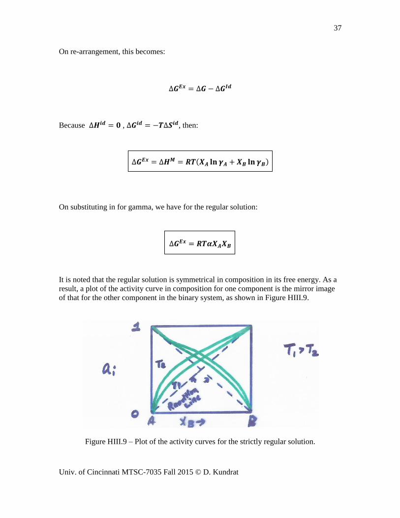
It is noted that the regular solution is symmetrical in composition in its free energy. As a

result, a plot of the activity curve in composition for one component is the mirror image

of that for the other component in the binary system, as shown in Figure HIII.9.

Figure HIII.9 – Plot of the activity curves for the strictly regular solution.

38


In case of a strictly regular solution, is not a function of temperature (note

that the temperature dependence for for a strictly regular solution is from the

(ideal) entropy portion). This means:

Note that .

Finally, we have:

Thus:

The Quasi-Chemical (QC) Model

This is the simplest fundamental model in which important atomistic factors are taken

into account. As a result, the parameters of the model have meaning.

Here, the individual atom to atom bond energies are summed as a distinct parameter. This

model not only predicts regular solution behavior under certain conditions, but the model

also anticipates both the tendency of real solutions towards ideality as , as well as

Henrian behavior as .

The energy of the solution is calculated by summing the short-range atom to atom

bonding energies. Consider one mole of A & B atoms in a crystal (noting ):

39


There are three types of bonds:

A-A bonds, each of energy ;

B-B bonds, each of energy ;

A-B bonds, each of energy .

Energies and are all negative quantities, which only approach zero when

atoms are separated by an infinite distance.

Let z be the co-ordination number, so that each atom has z nearest neighbors.

In our crystal,. there are:

number of A-A bonds;

number of B-B bonds;

number of A-B bonds.

Thus, the crystal the total energy (per mole) is:

The number of bonds P is evaluated as follows. Consider A atoms. The total number of

bonds is the number of A atoms times the number of bonds containing the A atom:

Thus, we have:

Re-arranging the above equation, we get:

40


Similarly, for the B atoms:

Or:

We now substitute for and in terms of and in our total energy:

It is clear that if A & B were un-mixed, then:

And

41


Thus, we have:

In this model, it is assumed that volume remains constant on mixing, thus:

Finally, we have for the QC model:

Obviously, the case where corresponds to the ideal solution, where:

Departure from ideality is summarized below:

42


Now, we want to calculate as a function of composition. The model assumes the

same random distribution of atoms as in an ideal solution.

Consider two neighboring lattice sites, labeled 1 and 2 in our model of the A-B crystal.

The probability that Site 1 is occupied by an atom of A is:

Similarly, the probability that Site 1 is occupied by a B atom is .

The probability that Site 1 is occupied by A when Site 2 is occupied by B is also .

The reverse – the probability that Site B is occupied by B when Site 2 is occupied by A is

also , thus the probability a neighboring pair of sites contain an A-B pair is .

In a similar fashion, that two neighboring sites contain an A-A pair is , or contain a B-

B pair is .

In total, there are

pairs of sites. Thus, the total number of A-B pairs is:

Or

Similarly, we have:

43


And

Finally, we have as a function of both bond energy differences and composition:

If we define:

Then, we have:

Where

We see that Ω from the QC model is exactly the empirical regular solution parameter

αRT, but, now, we have insight into its meaning and the compositional dependency

of .

We immediately see that the parabolic compositional term arises from the

probability of nearest neighboring sites being an A-B bond.

44


Now that we have confidence in the QC model, we want to express the partial

thermodynamic properties in terms of Ω. We already know the relationship between

molar and partial properties For enthalpy, we have (dropping notation M for molar):

And

Given the QC model, we now have:

Thus, we have:

Similarly, we have:

Finally, we have:

45


And

Also, we have:

And

Consider both Raoult’s Law and Henry’s Law for each component in solution AB in

terms of the QC model:

For component B, Raoult’s Law is satisfied by this model, since:

Henry’s Law is also satisfied as follows:

46


Generally, the equilibrium configuration of a solution is, at constant T and P, that which

minimizes , where is a measure of the effect of mixing relative to

unmixed components.

It is a compromise between and . If the latter is ideal, minimization of the term

always occurs at a 50-50 mixture, and increases to more negative values

with increasing temperature.

Enthalpy opposes this entropy effect if positive, and adds to it if negative, further

lowering free energy. This is illustrated in the following figures (HIII.10 (a) and (b)).

Figure HIII.10 (a) Enthalpy, entropy (multiplied by T) and Gibbs Free Energy changes

with composition, here for being positive. (b) Same as (a), but for being

negative. Note for both cases the symmetry about the 50-50 mixture.

For real solutions, varies in sign and magnitude, depending on the components. The

entropy change is close to ideal (within experimental verification) for many alloy systems

(for example, Sn-Ti) but departure can be rather significant in other systems, such as

oxide systems).

In the cases where there is significant departure, it is seen as a skewing of s plot of

To the right, or to the left of the 50-50 composition. If skewed by a small amount

(especially if within the experimental error), the QC model can be used to represent the

solution behavior, but, obviously, this becomes a limitation of this particular model.

In the QC model, A and B are assumed to mix randomly, yet is allowed to

accommodate a tendency to cluster, or to order. This appears to be somewhat

47


contradictory, but it is really a question of the degree of departure of from ideality!

This is discussed in greater detail below.

The critical parameters in the QC model are Ω and T, where refers to the bond energy

differences on mixing relative to un-mixing:

But, does not refer to the number of A-B pairs , which is assumed to be

random; viz.:

If is negative, this is a tendency toward ordering of A and B (ultimately leading to

compound formation, such as AB).

If is a large, negative number, the greater the tendency to ordering means the actual

should be larger than .

Because the actual is larger, the number of ways of arranging the atoms randomly on

the lattice is smaller, and decreases below the random value. Higher temperatures

help to maximize to compensate for smaller values.

If

, the model is not applicable.

If is positive – this being a tendency towards clustering of A to A and B to B – or,

phase separation. (In the extreme, this leads to complete immiscibility of A in B and B in

A.)

If is a large, positive number, this also means the actual is below , and

again, decreases because the number of ways to arrange the atoms on the lattice

decreases below the random number. To maximize , temperature again needs to be

increased. If , again, the model is not applicable.

48


Application of the GDE to Determine Activity

It is very commonly the situation that data is more easily measured for one component

than another.

However, a problem often exists when applying the GDE to activities, where it can be

asymmetric in the composition variable . This can be circumvented by working

with the activity coefficient rather than the activity:

This technique is illustrated in Figure HIII.11 (a) and (b).

Figure HIII.11 (a) Schematic of plot of log of the activity coefficient versus ratio of the

compositions – here the area under the curve is most generally finite.

(b) Illustration of the nature of log of the activity versus ratio of the components – the

area under the curve can be infinite.

A further aid in application of the GDE to obtain activity coefficient data for one

component from another is to introduce the following function:

49


This function has the benefit of being finite as when . In this application:

This function allows for evaluation of and , given and .

Note that no assumption has been made as to solution behavior, other than the fact that

is empirically the second-order term of a power series expansion, where the third

and higher-order terms are assumed to be insignificant. (The first-order terms are zero.) If

it turns out that , the solution over the composition region investigated may be

considered regular!)

The GDE provides an excellent illustration of thermodynamic consistency – of Raoult’s

and Henry’s Laws.; when the former applies for the solvent, the latter also applies for the

dilute solution for the solute.

For the Henrian solution composition range for Solute B, we have:

Thus, we have:

The GDE is for the binary system:

50


So, we have:

Integration of the above equation gives:

Since, by definition when , the constant must equal unity, regardless of

the value of near unity. Thus Raoult’s Law is obeyed for Solvent A when Henry’s Law is

obeyed for Solute B, and vice-versa.

PHASE EQUILIBRIA IN A ONE-COMPONENT SYSTEM

The remainder of this handout is devoted to phase equilibria, in the simplest – the one-

component - system. Consideration of the one-component diagram that includes pressure

stems naturally from the treatment of gases earlier in the present handout, since the

equilibria includes the gas phase as a stable phase in equilibrium with condensed phases.

Portrayal of phase equilibria for the one-component system typically employs T and P as

co-ordinates. Since there is no composition co-ordinate – the substance being pure – such

a depiction is not normally thought of as a phase diagram. This is because the two-

dimensional phase diagram normally encountered in materials involves temperature and

composition, but not pressure, as variables (pressure being constant at 1 atm for most

materials phase diagrams). But, multi-component phase diagram can also include

pressure, as is treated in Gaskell’s Chapter 14. The subsequent handout (HIV) treats two

or more components.

Variation of Gibbs Free Energy With Temperature

Consider Species A undergoing a phase change, such as melting:

51


For the system of solid and liquid A (where refers to the extensive Gibbs Free Energy:

Earlier, we had:

So that, at constant T,P:

Above the melting point of A

:

The above equation indicates the system becomes unstable, and melts, in which case:

52


Why? Because the phase with the lowest free energy is the more stable phase (for

example, the liquid phase is the more stable phase above the melting point).

Below

:

This situation is shown schematically in Figure HIII.12.

Figure HIII.12 – Schematic of molar Gibbs Free Energy of pure solid and liquid with

temperature (constant pressure).

Since we have:

And

53


The slope of the line in Figure HIII.12 corresponds to entropy.

Now consider the curvature of the line (i.e., change in slope):

If we subtract the two lines from each other, we get . This is depicted in

Figure HIII.13.

Figure HIII.13 – Schematic of Gibbs Free Energy of melting of a pure material with

temperature (constant pressure).

Figure HIII.13 can be summarized as:

54


Below

is positive Liquid is unstable

At

is zero L/S equilibrium

Above

is negative Solid is unstable

Since :

And

To know precisely , we must use enthalpy and entropy (via the Kirchoff

Square) to evaluate and

. But, if we assume

, then we have the following useful expressions:

Or

Variation of Gibbs Free Energy With Pressure

For most materials, molar volume increases on melting; not so for water, where .

From the expression , we have:

55


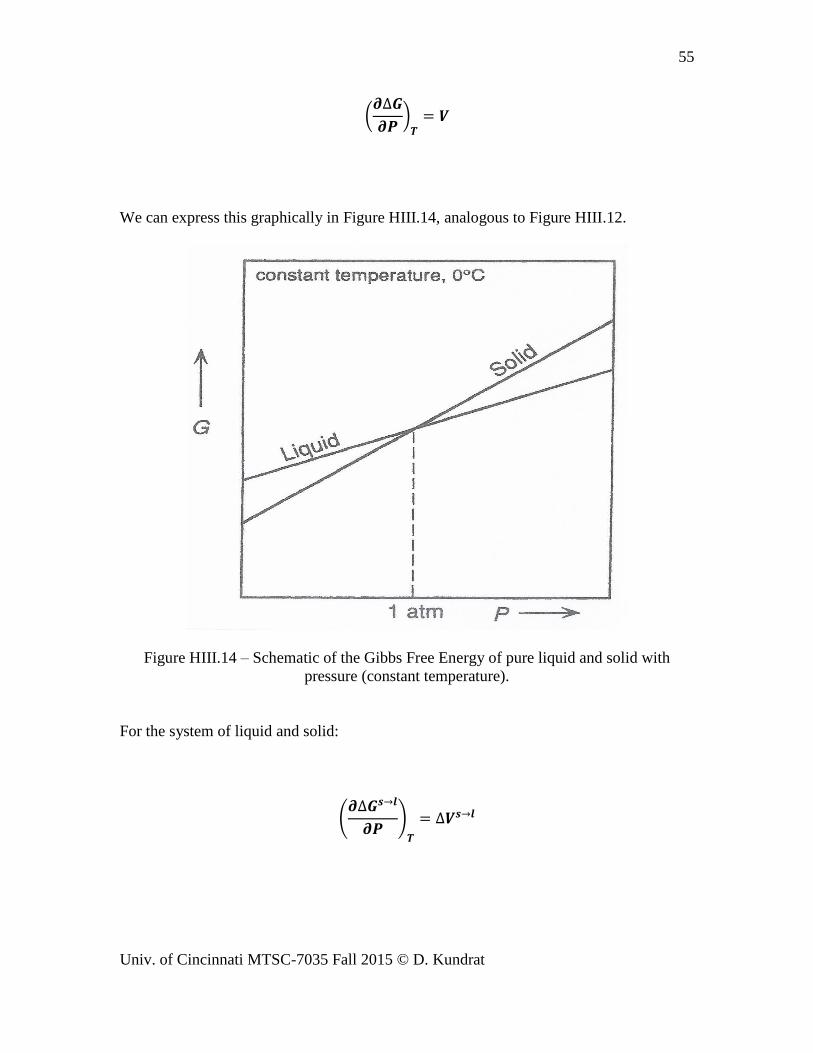
We can express this graphically in Figure HIII.14, analogous to Figure HIII.12.

Figure HIII.14 – Schematic of the Gibbs Free Energy of pure liquid and solid with

pressure (constant temperature).

For the system of liquid and solid:

56


Gibbs Free Energy As a function of Temperature and Pressure

In consideration of Figures HIII.12-14, it is clear that equilibrium between a solid and a

liquid of a pure substance could be maintained by simultaneously varying T vs. P,

keeping . The precise relationship between T and P at equilibrium can be

derived, as follows.

For any infinitesimal (i.e., reversible) change in T and P:

At equilibrium , thus, we get the Claperyon Equation:

The Claperyon Equation is not restricted to just to the liquid/solid equilibrium, but

equilibrium between any two phases.

For all materials is positive; for most materials on melting is also positive,

so generally is positive. However, for water is negative. Thus, for most

materials, as pressure is increased, the melting point increases; for water, as pressure

increases, its melting point decreases. (That is why skating on ice works – the pressure of

your body weight melts and lubricates the contact area between the blade and the ice.)

Figure HIII.15 shows the melting point range for pure water as a function of T and P

(points m-o).

57


Figure HIII.15 – Gibbs Free Energies of pure solid and liquid water as a function of T

and P.

Saturated Vapor Pressure

If the molar volume of the condensed phase (l or s) is much smaller than that of the

equilibrium vapor pressure, then, without much error, we can state:

In addition, if it can be assumed that the vapor phase behaves as an ideal gas (where

) then, the Claperyon Equation can be modified into the Clasius-Claperyon

Equation:

58


Or

Finally, if

, then , so, on integration, we have:

The value of P from this equation is the saturated vapor pressure exerted by the

condensed phase in equilibrium with the vapor phase at temperature T. In this equation,

refers to the heat of evaporation.

The Phase Diagram for the One-Component System and the Gibbs Phase Rule

The effect of T and P on the solid/liquid; solid/vapor and liquid/vapor equilibria of a pure

component when displayed in a plot constitutes a phase diagram for the one-component

system. This phase diagram for water is shown in Figure HIII.16.

59


Figure HIII.16 – Log-log schematic plot of the P-T phase diagram for H2O.

For the l/s line (i.e., the line of saturation of the l/s equilibrium) is calculated from the

Claperyon Equation of the form:

For water, is generally a function of temperature, unless it is assumed that

.

It is seen that the intersection of all three lines of saturation occurs at a precise T and P

(viz.: 0.006 atm and 0.0075 °C). This is a unique (invariant) point called the triple point

(labeled O in figure HIII.16). Obviously, if only two of the lines of saturation are

known/calculated, their intersection identifies the triple point, so that the third line of

saturation must begin there.

This figure also illustrates what is known as a guiding principle in the construction and

interpretation of phase diagrams: the Gibbs Phase Rule (GPR). The lines in this figure are

60


identified as Lines OA, OB and OC. These divide the phase diagram into three areas,

within each of which only one phase is stable. This means that within any one of these

domains, temperature and pressure can be varied independently, and the domain for the

single phase remains stable. Thus, this particular equilibrium – the single phase domain –

has two degrees of freedom, which means that the two variables of P and T can be varied

independently. The lines OA, OB and OC delineate the boundaries of the single-phase

domain. On any of these three boundary lines, if T or P is varied, the other must follow

suit. This means that there is now only one degree of freedom. Finally, at the unique

(invariant) triple point, there is no single variable (T or P) to be varied; it occurs at a

unique value of T and P, corresponding to zero degrees of freedom.

The GPR can be stated as:

In the above equation, is the degrees of freedom; is the number of components (here,

equal to one) and is the number of phases participating in the equilibrium.

As an example, for the single phase region in the one-component system, , thus

; for the boundary lines, ; finally, for the triple

point, .

Solid/Solid Equilibria in the One-Component System

Elements that exhibit one or more crystal structures are called alloptropic (for

compounds, it is called polymorphic). Figure HIII.17 shows the variation of the vapor

pressure of pure iron with temperature, where there are three triple points: α (BCC)/ γ

(FCC)/v; γ (FCC)/δ (BCC)/v and δ (BCC)/l/v. Note the slope of the α/γ equilibrium line,

which is negative. This means that a decrease of compared to . Likewise, the line

for the γ/δ equilibrium is positive, indicating is greater than .

61


Figure HIII.17 – The phase diagram for pure iron

In the following figure (HIII.18), the variation of the molar Gibbs Free Energy for the

BCC, FCC, liquid and vapor phases of iron are shown as a function of T, P. Here, it is

seen that the slope corresponding to each phase progressively increase

with T. This indicates that the entropy of the solid phase at higher temperatures is larger

than at lower temperatures.

62


Figure HIII.18 – Schematic representation of the variation of the molar Gibbs Free

Energy of the BCC, FCC, liquid and vapor phases of iron with temperature at constant

pressure.

Finally, back to water, the phase diagram at very high pressures and a range of

temperatures from -60 to 40 °C is given in Figure HIII.19. Clearly, there are five different

crystal structures for ice!

Figure HIII.19 – The P-T phase diagram for water, showing five crystal structures for ice.

63


The P-T-V Phase Diagram for the One-Component System

The phase diagram for any one-component system need not be restricted to just P and T

as variables, but also may include molar volume V.

Earlier, we illustrated (Figure HIII.1) a version of this, showing the existence of a region

of liquefaction for a gas. The critical temperature represents the limit of liquefaction in

this diagram, and it is actually a phase diagram.

In point of fact, any pure substance exhibits such behavior as shown in this phase

diagram for a gas, albeit, at, possibly extreme temperatures, extreme pressures, or both!

So, Figure HIII.1 is reproduced here as Figure HIII.20 to represent any pure substance on

a P-V plot with isotherms.

Figure HIII.20 – Isotherms in a P-V phase diagram of a pure substance.

So, the P-T phase diagrams shown earlier can be expanded to include V as a third

variable, producing a 3-D phase diagram as P-T-V space.

Volume →

64


Figure (HIII.21) shows such a plot (here, schematically) for a substance that contracts on

melting (such as water). Also, note that the original P-T plot for water (Figure HIII.15) is

log-log.

Figure HIII.21 – A schematic P-V-T phase diagram for a pure substance that contracts on

melting, where is temperature.

The final figure (HIII.22) shows the actual 3-D plot for water, with the various differing

structural form of ice, and corresponding triple points. Note that the scale here is not log-

log, thus Figure HIII.16 does not directly correspond.

65


Figure HIII.22 – The actual P-V-T phase diagram for water.

66


Date post:	02-Apr-2022
Category:	Documents
Upload:	others
View:	12 times
Download:	0 times

ADVANCED THERMODYNAMICS Handout III Behavior of Gases ...

Documents