Advanced Topics in Numerical Analysis: High Performance Computing More distributed memory algorithms Georg Stadler, Dhairya Malhotra Courant Institute, NYU Spring 2019, Monday, 5:10–7:00PM, WWH #1302 May 6, 2019 1 / 27
Transcript
Advanced Topics in Numerical Analysis:High Performance Computing
More distributed memory algorithms
Georg Stadler, Dhairya MalhotraCourant Institute, NYU
Spring 2019, Monday, 5:10–7:00PM, WWH #1302
May 6, 2019
1 / 27
Outline
Organization issues
Summary of previous class
Multigrid
2 / 27
Organization
Scheduling:I Homework assignment #6 posted last week, due next Monday.I How are your final projects coming along? Special office hours
for final project this week: Wednesday 1-2pm and Thursdaynoon-1pm in office #1111. Come by!
Topics today:I Partitioning and balancing: space filling curvesI Multigrid
3 / 27
Outline
Organization issues
Summary of previous class
Multigrid
4 / 27
Partitioning and Load Balancing
Thanks to Marsha Berger for letting me use many of her slides. Thanksto the Schloegel, Karypis and Kumar survey paper and the Zoltan
website for many of these slides and pictures.
5 / 27
Partitioning
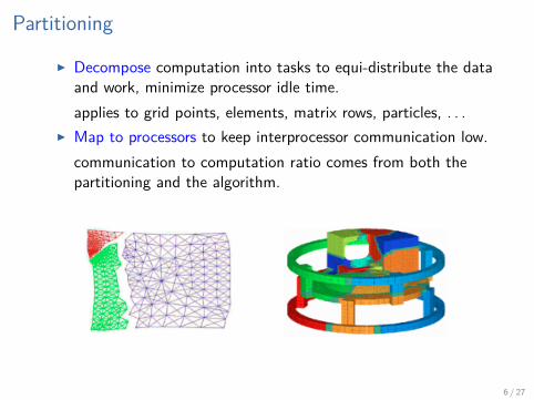
I Decompose computation into tasks to equi-distribute the dataand work, minimize processor idle time.applies to grid points, elements, matrix rows, particles, . . .
I Map to processors to keep interprocessor communication low.communication to computation ratio comes from both thepartitioning and the algorithm.
I Data distributed among the processorsI Data distribution defines work assignmentI Owner performs all computations on its data.I Data dependencies for data items owned by different
processors incur communication
7 / 27
Partitioning
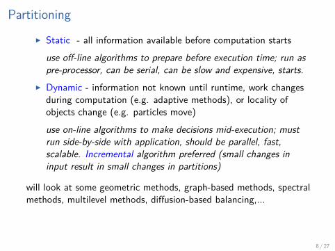
I Static - all information available before computation starts
use off-line algorithms to prepare before execution time; run aspre-processor, can be serial, can be slow and expensive, starts.
I Dynamic - information not known until runtime, work changesduring computation (e.g. adaptive methods), or locality ofobjects change (e.g. particles move)
use on-line algorithms to make decisions mid-execution; mustrun side-by-side with application, should be parallel, fast,scalable. Incremental algorithm preferred (small changes ininput result in small changes in partitions)
will look at some geometric methods, graph-based methods, spectralmethods, multilevel methods, diffusion-based balancing,...
8 / 27
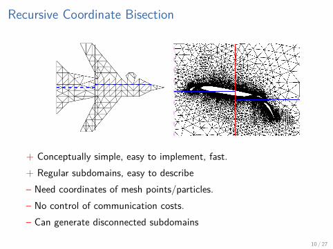
Recursive Coordinate Bisection
Divide work into two equal parts using cutting plane orthogonal tocoordinate axis For good aspect ratios cut in longest dimension.
1st cut
2nd
2nd
3rd
3rd 3rd
3rd
Geometric Partitioning
Applications of Geometric Methods
Parallel Volume Rendering
Crash Simulations and Contact Detection
Adaptive Mesh Refinement Particle Simulations
Can generalize to k-way partitions. Finding optimal partitions isNP hard. (There are optimality results for a class of graphs as agraph partitioning problem.)
9 / 27
Recursive Coordinate Bisection
+ Conceptually simple, easy to implement, fast.+ Regular subdomains, easy to describe– Need coordinates of mesh points/particles.– No control of communication costs.– Can generate disconnected subdomains
10 / 27
Recursive Coordinate Bisection
Implicitly incremental - small changes in data result in smallmovement of cuts
11 / 27
Recursive Inertial Bisection
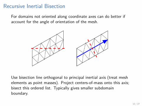
For domains not oriented along coordinate axes can do better ifaccount for the angle of orientation of the mesh.
Use bisection line orthogonal to principal inertial axis (treat meshelements as point masses). Project centers-of-mass onto this axis;bisect this ordered list. Typically gives smaller subdomainboundary.
12 / 27
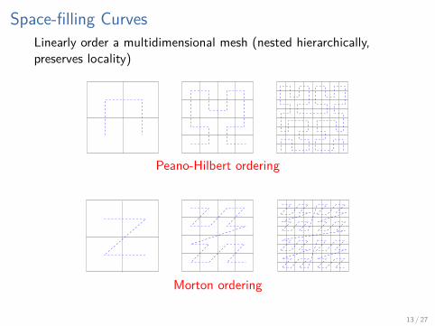
Space-filling CurvesLinearly order a multidimensional mesh (nested hierarchically,preserves locality)
Peano-Hilbert ordering
Morton ordering
13 / 27
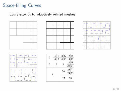
Space-filling Curves
Easily extends to adaptively refined meshes
1
3
2827
26 2524 23222120
19 18171615
13 141211
10
98
765
4
2
14 / 27
Space-filling Curves
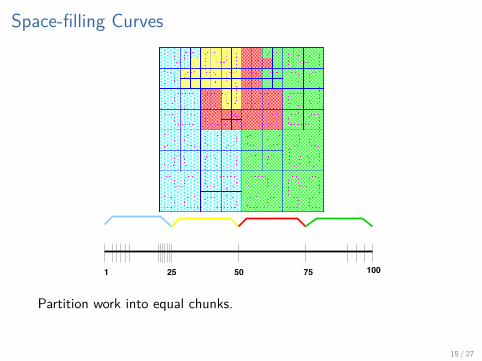
1 25 50 75 100
Partition work into equal chunks.
15 / 27
Space-filling Curves
+ Generalizes to uneven work loads - incorporate weights.+ Dynamic on-the-fly partitioning for any number of nodes.+ Good for cache performance
16 / 27
Space-filling Curves
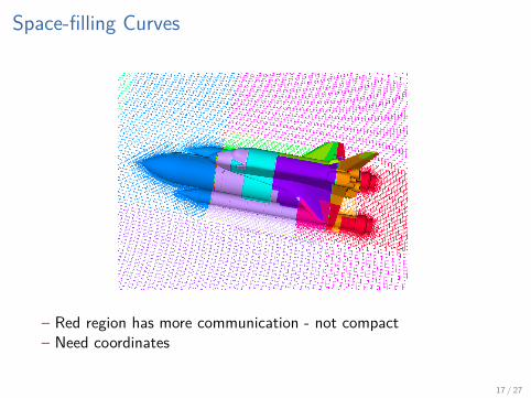
– Red region has more communication - not compact– Need coordinates
17 / 27
Space-filling Curves
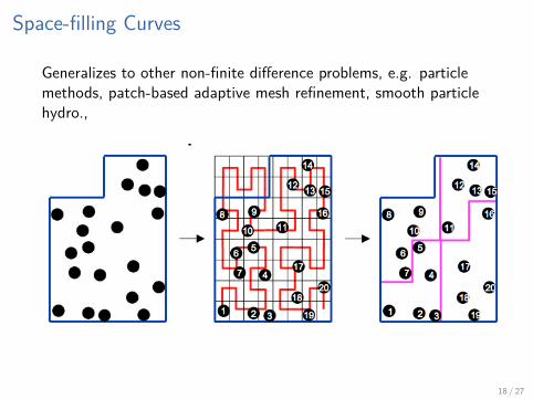
Generalizes to other non-finite difference problems, e.g. particlemethods, patch-based adaptive mesh refinement, smooth particlehydro.,
18 / 27
Space-filling Curves
Implicitly incremental - small changes in data results in smallmovement of cuts in linear ordering
19 / 27
Morton Ordering
Computing Morton Indedx:I convert coordinate to integersI interleave the bits to generate a new integerI works for arbitrary dimension (1D, 2D, 3D, 4D, ...)
20 / 27
Application to N-body codes
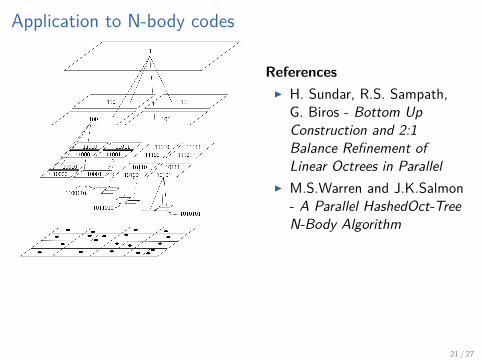
ReferencesI H. Sundar, R.S. Sampath,
G. Biros - Bottom UpConstruction and 2:1Balance Refinement ofLinear Octrees in Parallel
I M.S.Warren and J.K.Salmon- A Parallel HashedOct-TreeN-Body Algorithm
21 / 27
Application to N-body codes
Parallel Tree ConstructionI compute Morton Ids of
particles;I parallel sort and partition
across processesI construct local tree on each
processI adjust for overlapping tree
nodes at process boundaries.
21 / 27
Application to N-body codes
CommunicationI all processes store the
starting Morton IDs of eachpartition
I to fetch a data element withgiven coordinates, we candetermine the process ID tocommunicate with using abinary search in the list ofstarting Morton IDs(O(log p) cost).
21 / 27
Visualization
I Useful for interpreting results.I Can also be helpful for debugging!
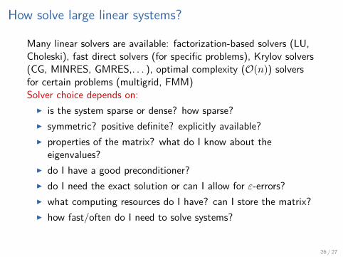
Many linear solvers are available: factorization-based solvers (LU,Choleski), fast direct solvers (for specific problems), Krylov solvers(CG, MINRES, GMRES,. . . ), optimal complexity (O(n)) solversfor certain problems (multigrid, FMM)Solver choice depends on:
I is the system sparse or dense? how sparse?I symmetric? positive definite? explicitly available?I properties of the matrix? what do I know about the
eigenvalues?I do I have a good preconditioner?I do I need the exact solution or can I allow for ε-errors?I what computing resources do I have? can I store the matrix?I how fast/often do I need to solve systems?
26 / 27
Reading/Sources
Why Multigrid Methods are so efficient:http://www.cs.technion.ac.il/people/irad/
Algorithms for 2D/3D Poisson Equation with n unknowns
Algorithm 2D (n= N2) 3D (n=N3) ° Dense LU n3 n3 ° Band LU n2 n7/3 ° Explicit Inv. n2 n2 ° Jacobi/GS n2 n2
° Sparse LU n 3/2 n2 ° Conj.Grad. n 3/2 n 3/2 ° RB SOR n 3/2 n 3/2 ° FFT n*log n n*log n
° Multigrid n n ° Lower bound n n
Multigrid is much more general than FFT approach (many elliptic PDE)
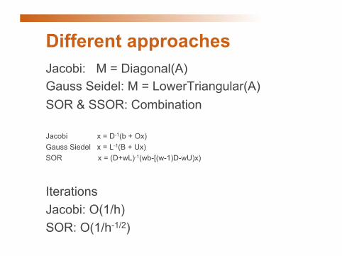
Different approaches Jacobi: M = Diagonal(A) Gauss Seidel: M = LowerTriangular(A) SOR & SSOR: Combination Jacobi x = D-1(b + Ox) Gauss Siedel x = L-1(B + Ux) SOR x = (D+wL)-1(wb-[(w-1)D-wU)x)
Iterations Jacobi: O(1/h) SOR: O(1/h-1/2)
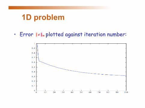
1D problem
Eigenvectors
Error /eigenvectors
Error for high frequencies
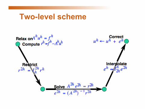
Two-level scheme
Prolongation
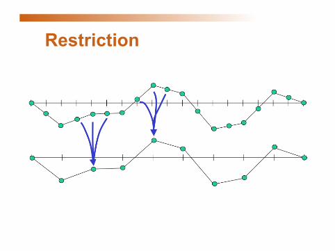
Restriction
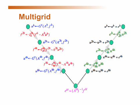
V-cycle
Multigrid
Full multigrid (O(N))
COARSE GRID
FINE GRID
Parallelizing multigrid Regular grids • grid coarsening is trivial • grid partitioning is trivial • coloring can be constructed analytically • smoother Unstructured grids/graphs • graph coarsening Multigrid for generic matrices
Algebraic multigrid Define coarse grid in terms of strengths of
connections Use MIS to define nodes No need to create new edges Interpolation and restriction operations
based on the smooth error idea Only requires matrix entries Works for graph Laplacians