Advection / Hyperbolic PDEs - Stony Brook...

PHY 688: Numerical Methods for (Astro)Physics

Advection / Hyperbolic PDEs


Notes● In addition to the slides and code examples, my notes on PDEs with

the finite-volume method are up online:– https://github.com/Open-Astrophysics-Bookshelf/numerical_exercises


Linear Advection Equation● The linear advection equation provides a simple problem to explore

methods for hyperbolic problems

– Here, u represents the speed at which information propagates● First order, linear PDE

– We'll see later that many hyperbolic systems can be written in a form that looks similar to advection, so what we learn here will apply later.


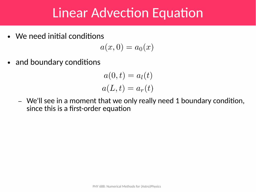
Linear Advection Equation● We need initial conditions

● and boundary conditions

– We'll see in a moment that we only really need 1 boundary condition, since this is a first-order equation


Linear Advection Equation● Solution is trivial—any initial configuration simply shifts to the right

(for u > 0 )– e.g. a(x - ut) is a solution– This demonstrates that the solution is constant on lines x = ut –these

are called the characteristics● This makes the advection problem an ideal test case

– Evolve in a periodic domain– Compare original profile with evolved profile after 1 period– Differences are your numerical error


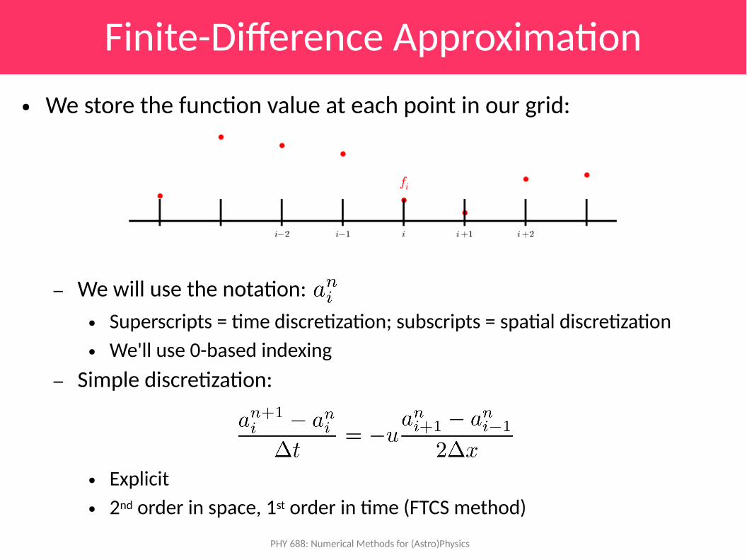
Finite-Difference Approximation● We store the function value at each point in our grid:

– We will use the notation:● Superscripts = time discretization; subscripts = spatial discretization● We'll use 0-based indexing

– Simple discretization:

● Explicit● 2nd order in space, 1st order in time (FTCS method)


Boundary Conditions● We want to be able to apply the same update equation to all the grid

points:

– Here, C = uΔt / Δx is the fraction of a zone we cross per timestep—this is called the Courant-Friedrichs-Lewy number (or CFL number)

● Notice that if we attempt to update zone i = 0 we “fall off” the grid● Solution: ghost points (for finite-volume, we'll call them ghost cells)

Grid for N points


Boundary Conditions● Before each timestep, we will the ghost points with data the

represents the boundary conditions

– Note that with this discretization, we have a point exactly on each boundary (we only really need to update one of them)

– Periodic BCs would mean:●

– Other common BCs are outflow (zero derivative at boundary)

General grid of N points


Implementation and Testing● Recall that the solution is to just propagate any initial shape to the

right:

– We'll code this up with periodic BCs and compare after 1 period– On a domain [0,1], one period is simply: 1/u

● We'll use a tophat initial profile● Let's look at the code...

code: fdadvect.py


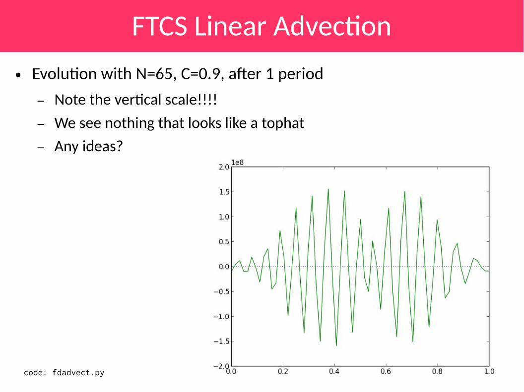
FTCS Linear Advection● Evolution with N=65, C=0.9, after 1 period

– Note the vertical scale!!!!– We see nothing that looks like a tophat– Any ideas?

code: fdadvect.py


FTCS Linear Advection● Reducing the timestep is equivalent to reducing the CFL number

– CFL = 0.1, still 1 full period– The scale is much

reduced, but it is still horrible

– Let's look how these features develop

code: fdadvect.py


FTCS Linear Advection● Here we evolve for only 1/10th of a period

– CFL = 0.1– Notice that the

oscillations are developing right near the discontinuities

– So far we've looked at timestep, what about resolution?

code: fdadvect.py


FTCS Linear Advection● This is with N = 257 points

– There is something more fundamental than resolution or CFL number going on here...

code: fdadvect.py


Stability● The problem is that FTCS is not stable● There are a lot of ways we can investigate the stability

– It is instructive to just work through an update using pencil + paper to see how things grow

– Growth of a single Fourier mode– Truncation analysis– Graphically: we can trace back the characteristics to see what

information the solution depends on.


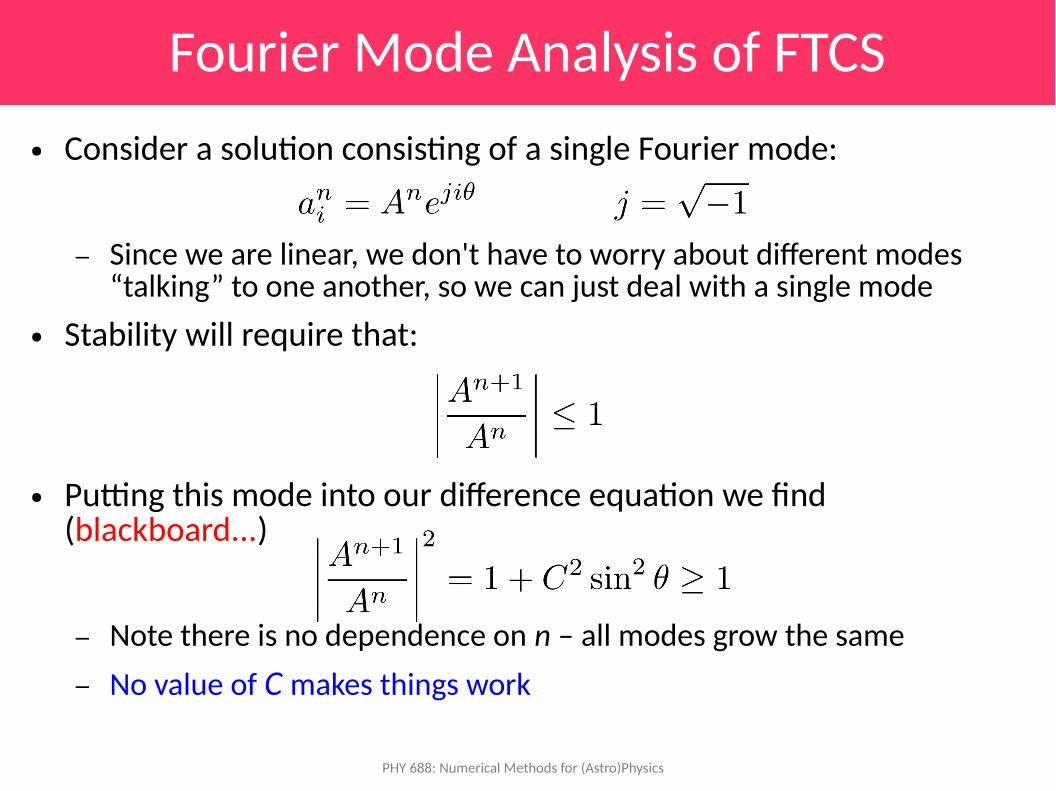
Fourier Mode Analysis of FTCS● Consider a solution consisting of a single Fourier mode:

– Since we are linear, we don't have to worry about different modes “talking” to one another, so we can just deal with a single mode

● Stability will require that:

● Putting this mode into our difference equation we find (blackboard...)

– Note there is no dependence on n – all modes grow the same– No value of C makes things work


Fourier Mode Analysis of FTCS● FTCS is unconditionally unstable● Note that although this method of stability analysis only works for

linear equations, it can still guide our insight into nonlinear equations

● This methodology was developed by von Neumann during WWII at LANL and allegedly, it was originally classified...


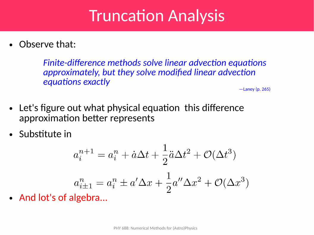
Truncation Analysis● Observe that:

● Let's figure out what physical equation this difference approximation better represents

● Substitute in

● And lot's of algebra...

Finite-difference methods solve linear advection equations approximately, but they solve modified linear advection equations exactly

—Laney (p. 265)


Truncation Analysis● We find:

– We are more accurately solving an advection/diffusion equation– But the diffusion is negative!

● This means that it acts to take smooth features and make them strongly peaked—this is unphysical!

– The presence of a numerical diffusion (or numerical viscosity) is quite common in difference schemes, but it should behave physically!

This is our original equation

This looks like diffusion, but look at the sign!


Upwinding● Let's go back to the original equation and try a different

discretization● Instead of a second-order (centered-difference) spatial difference,

let's try first order.– We have two choices:

● Let's try the upwinded difference—that gives:upwind downwind


Upwinding● Upwinding solution with N = 65, C = 0.9, after 1 period

– Much better– There still is some error, but it is not unstable– Numerical diffusion is

evident

code: fdadvect.py


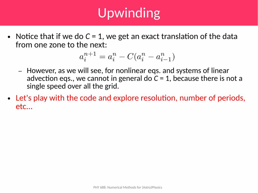
Upwinding● Notice that if we do C = 1, we get an exact translation of the data

from one zone to the next:

– However, as we will see, for nonlinear eqs. and systems of linear advection eqs., we cannot in general do C = 1, because there is not a single speed over all the grid.

● Let's play with the code and explore resolution, number of periods, etc...


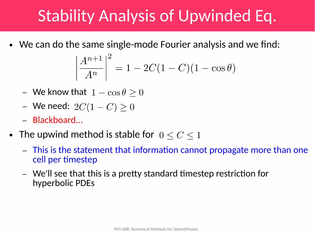
Stability Analysis of Upwinded Eq.● We can do the same single-mode Fourier analysis and we find:

– We know that – We need: – Blackboard...

● The upwind method is stable for – This is the statement that information cannot propagate more than one

cell per timestep– We'll see that this is a pretty standard timestep restriction for

hyperbolic PDEs


Stability Analysis of Upwinded Eq.● Truncation analysis would show this method is equivalent to

– Represents physical diffusion so long as 1 – C > 0– This also shows that we get the exact solution for C = 1

● Note that if we used the downwind difference, our method would be unconditionally unstable– Direction of difference based on sign of velocity

● Physically, the choice of upwinding means that we make use of the information from the direction the wind is blowing– This term originated in the weather forecasting community


Phase Error● Examining the behavior of a Fourier mode can also tell us if the

method introduces a phase lag– Look at the ratio of imaginary to real parts of the amplification factor– Some methods have severe phase lag– We won't go into this here...


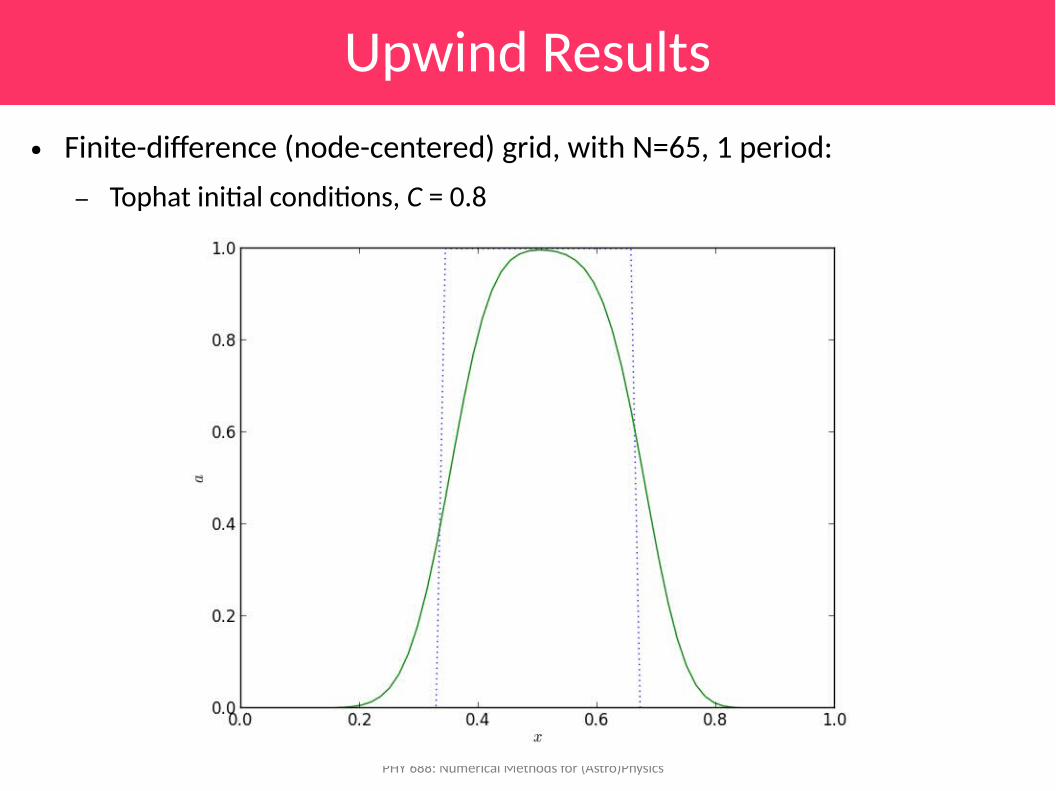
Upwind Results● Finite-difference (node-centered) grid, with N=65, 1 period:

– Tophat initial conditions, C = 0.8


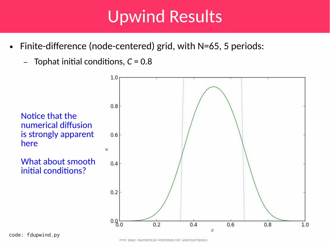
Upwind Results● Finite-difference (node-centered) grid, with N=65, 5 periods:

– Tophat initial conditions, C = 0.8

Notice that the numerical diffusion is strongly apparent here

What about smooth initial conditions?

code: fdupwind.py


Upwind Results● Finite-difference (node-centered) grid, with N=65, 1 period:

– sine wave, C = 0.8

code: fdupwind.py


Upwind Results● Finite-difference (node-centered) grid, with N=65, 5 periods

– sine wave, C = 0.8

Note that the sine wave stays in phase (that's a good thing)

Diffusion still apparent.

Just for fun, let's try a downwinded method...

code: fdupwind.py


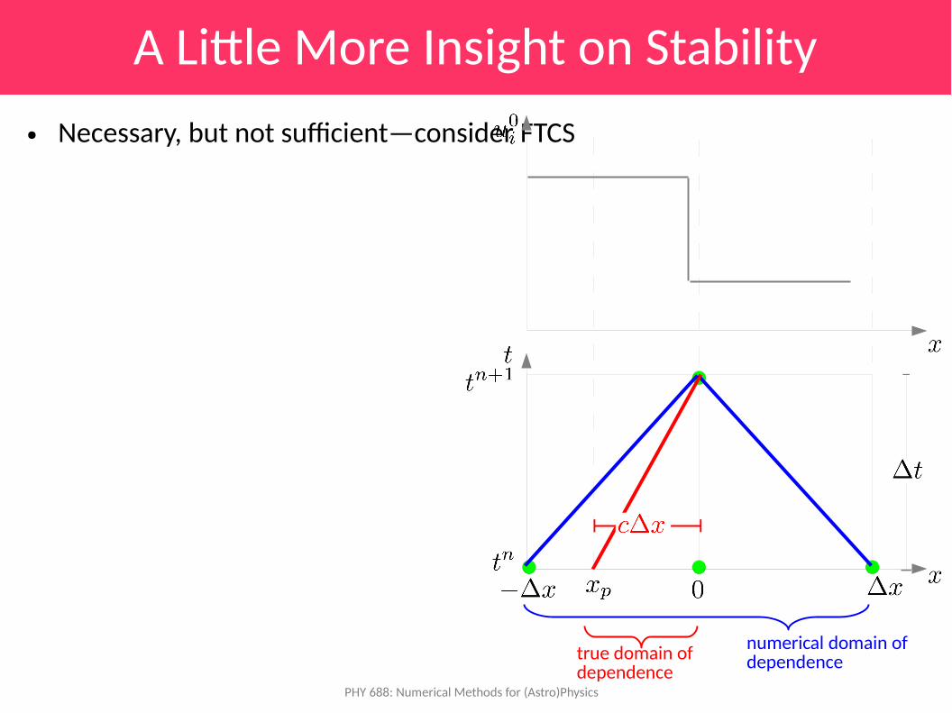
A Little More Insight on Stability● A necessary (but not sufficient) condition for stability is that the

numerical domain of dependence contain the true domain of dependence (see Lahey, Ch. 12 for a nice discussion)

– True domain of dependence is found by tracing the characteristics backwards in time

true domain of dependence

numerical domain of dependence

Upwind method ►For u > 0


A Little More Insight on Stability● The downwind method clearly

violates this● Ex from Lahey:

– Consider initially discontinuous data

– True solution at x = 0 is a01 = 1 – Downwind method:

gives:

numerical domain of dependence

true domain of dependence

The numerical domain of dependence doesn't include the true domain of dependence, and we get the wrong answer.


A Little More Insight on Stability● Necessary, but not sufficient—consider FTCS

numerical domain of dependencetrue domain of

dependence


Implicit Differencing● If we discretize the spatial derivative using information at the new

time, then we get an implicit method– Unconditionally stable– You'll explore this on your homework


Other Finite-Difference Methods● There are many other finite-difference methods that build off of what

we already saw● Lax-Friedrichs:

– Start with FTCS:– Simple change, replace:– We get:

– This is stable for C < 1, but notice that it doesn't contain the point we are updating! (Let's explore this...)

● Can suffer from odd-even decoupling● Can be more diffusive than upwinding (and gets worse for smaller C)

● You'll explore Lax-Wendroff in your homework—it is second order in space and time. Works well, but can oscillate...


Measuring Convergence● As we move to higher-order methods, we will want to measure the

convergence of our methods– We have data at N points for each time level– We need a norm that operates on the gridded data. A popular choice

is the L2 norm:

– Using the grid width ensure that this measure is resolution independent

– We can take the error of our method to be:


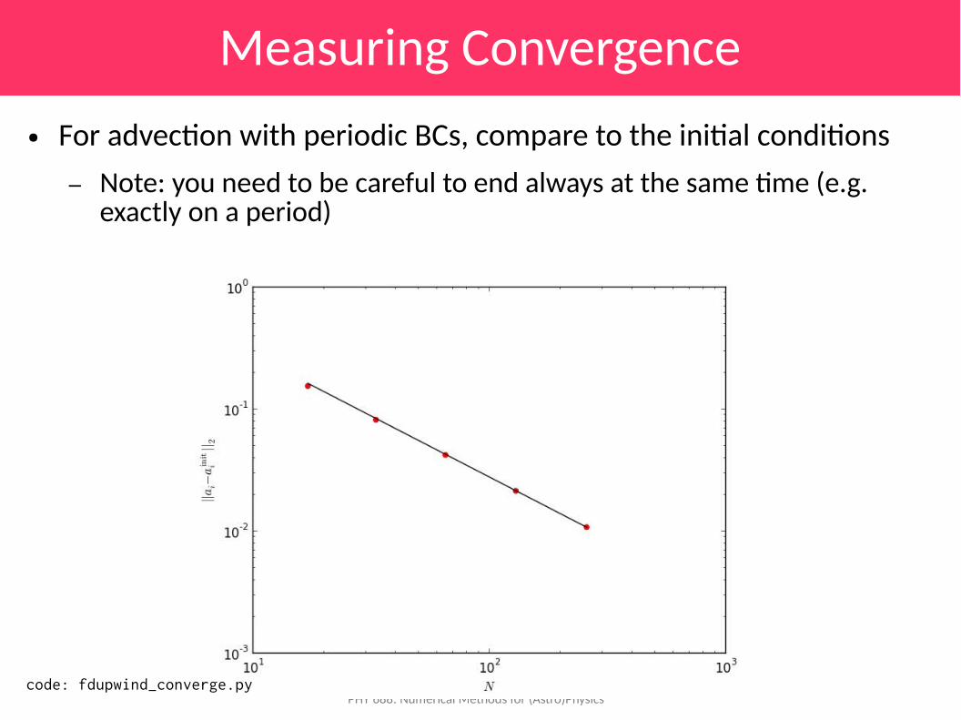
Measuring Convergence● For advection with periodic BCs, compare to the initial conditions

– Note: you need to be careful to end always at the same time (e.g. exactly on a period)

code: fdupwind_converge.py


Grid Types

“Regular” finite-difference grid. Data is associate with nodes spaced Δx apart. Note that here we can have a point exactly on the boundary

Cell-centered finite-difference grid. Here we consider cells of with Δx and associate the data with a point at the center of the cell. Note that data will be Δx/2 inside the boundary

Finite-volume grid—similar to the cell-centered grid, we divide the domain into cells/zones. Now we store the average value of the function in each zone.


Grid Types● Finite-difference

– Some methods use staggered grids: some variables are on the nodes (cell-boundaries) some are at the cell centers

– Boundary condition implementation will differ depending on the centering of the data

– For cell-centered f-d grids: ghost cells implement the boundary conditions

● Finite-volume– This is what we'll focus on going forward– Very similar in structure to cell-centered f-d, but the interpretation of

the data is different.


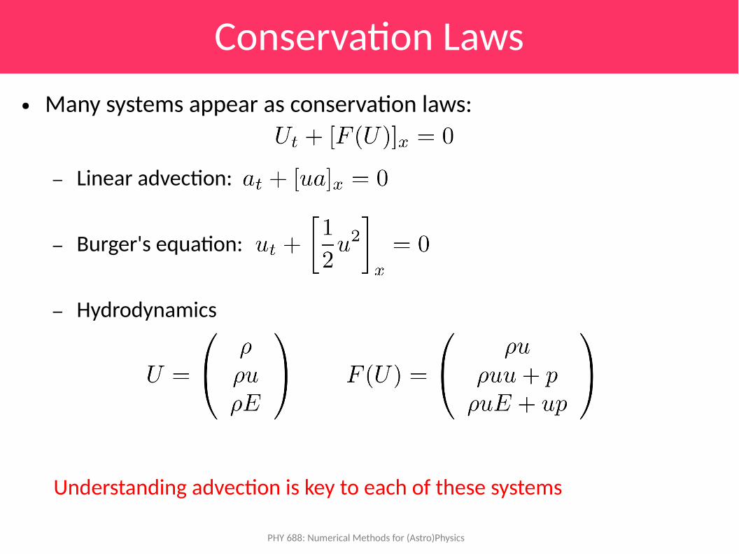
Conservation Laws● Many systems appear as conservation laws:

– Linear advection:

– Burger's equation:

– Hydrodynamics

Understanding advection is key to each of these systems


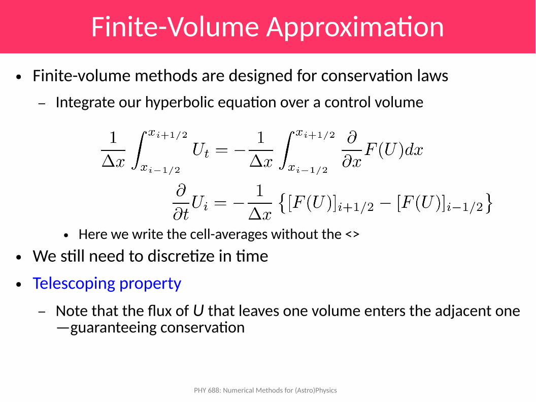
Finite-Volume Approximation● Finite-volume methods are designed for conservation laws

– Integrate our hyperbolic equation over a control volume

● Here we write the cell-averages without the <>● We still need to discretize in time● Telescoping property

– Note that the flux of U that leaves one volume enters the adjacent one—guaranteeing conservation


Finite-Volume Approximation● A second-order approximation for our advection equation is

– Notice that the RHS is centered in time● To complete this method, we need to compute the fluxes on the

edges– We can do this in terms of the interface state

– Now we need to find the interface state. There are two possibilities: coming from the left or right of the interface


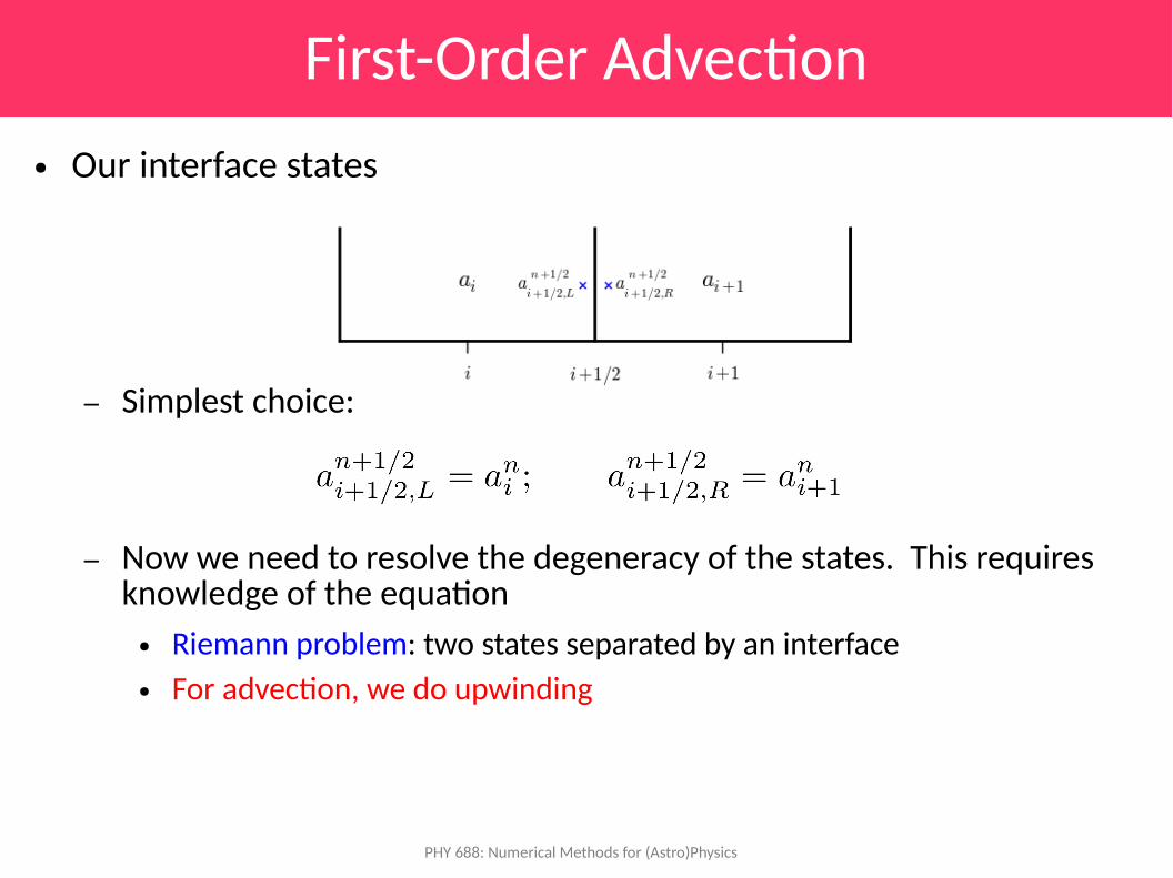
First-Order Advection● Our interface states

– Simplest choice:

– Now we need to resolve the degeneracy of the states. This requires knowledge of the equation

● Riemann problem: two states separated by an interface● For advection, we do upwinding


First-Order Advection● Riemann problem (upwinding):

– This is simple enough that we can write out the resulting update (for u > 0):

– This is identical to the first-order upwind finite-difference discretization we already studied


Second-Order Advection● Going to second-order requires making the interface states second-

order in space and time – We will use a piecewise linear reconstruction of the cell-average data

to approximate the true functional form– We Taylor expand in space and time to find the time-centered,

interface state● Let's derive this on the blackboard...


Second-Order Advection● Tophat with 64 zones, C = 0.8

Notice the oscillations—they seem to be associated with the steep jumps

code: fv_advection.py


Second-Order Advection● Gaussian with 64 zones, C = 0.8

This looks nice and smooth



Second-Order Advection● Remember—you should always look at the convergence of your code

—if you do not get what you are supposed to get, you probably have a bug (or you don't understand the method well enough...)

Convergence for the Gaussian



Second-Order Advection● General notes:

– We derived both the left and right state at each interface—for advection, we know that we are upwinding, so we only really need to do the upwinded state

– But, for a general conservation law, the upwind direction can change from zone to zone and timestep to timestep AND there can be multiple waves (e.g. systems), so for the general problem, we need to compute both states

● If you set the slopes to 0, you reduce to the first-order method


Second-Order Advection● We need 2 ghost cells on each end:

● Let's look at the code...

The state here depends on the slope in zone lo-1

This slope requires the data from the zones on either size of it


Design of a General Solver● Simulation codes for solving conservation laws generally follow the

following flow:– Set initial conditions– Main evolution loop (loop until final time reached)

● Fill boundary conditions● Get the timestep● Compute the interface states● Solve the Riemann problem● Do conservative update

● We'll see that this same procedure can be applied to nonlinear problems and systems (like the equations of hydrodynamics)


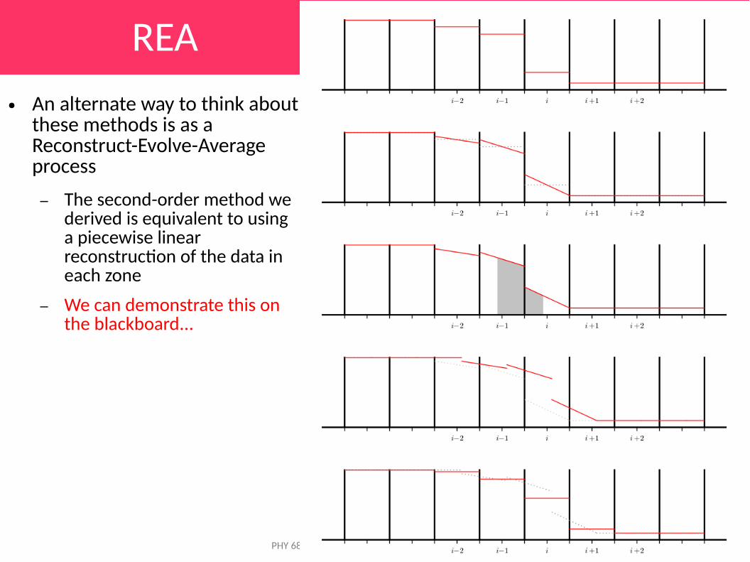
REA● An alternate way to think about

these methods is as a Reconstruct-Evolve-Average process

– The second-order method we derived is equivalent to using a piecewise linear reconstruction of the data in each zone

– We can demonstrate this on the blackboard...


No-limiting Example

Here we see an initial discontinuity advected using a 2nd-order finite-volume method, where the slopes were taken as unlimited centered differences. Note the overshoot and undershoots


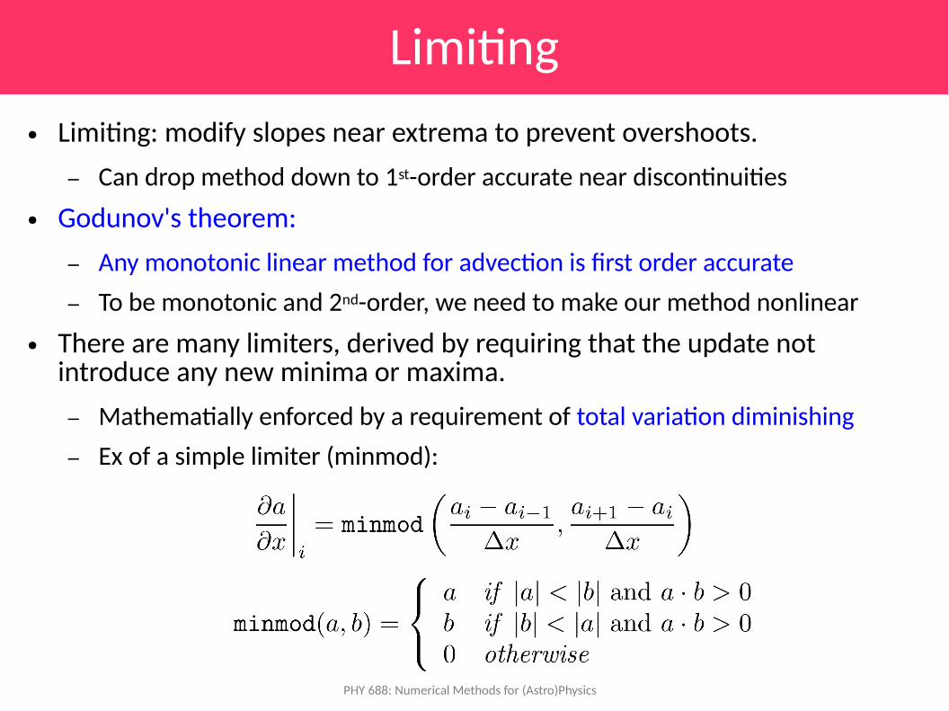
Limiting● Limiting: modify slopes near extrema to prevent overshoots.

– Can drop method down to 1st-order accurate near discontinuities● Godunov's theorem:

– Any monotonic linear method for advection is first order accurate– To be monotonic and 2nd-order, we need to make our method nonlinear

● There are many limiters, derived by requiring that the update not introduce any new minima or maxima. – Mathematially enforced by a requirement of total variation diminishing– Ex of a simple limiter (minmod):


Limiting Example

This is the same initial profile advected with limited slopes. Note that the profile remains steeper and that there are no oscillations.


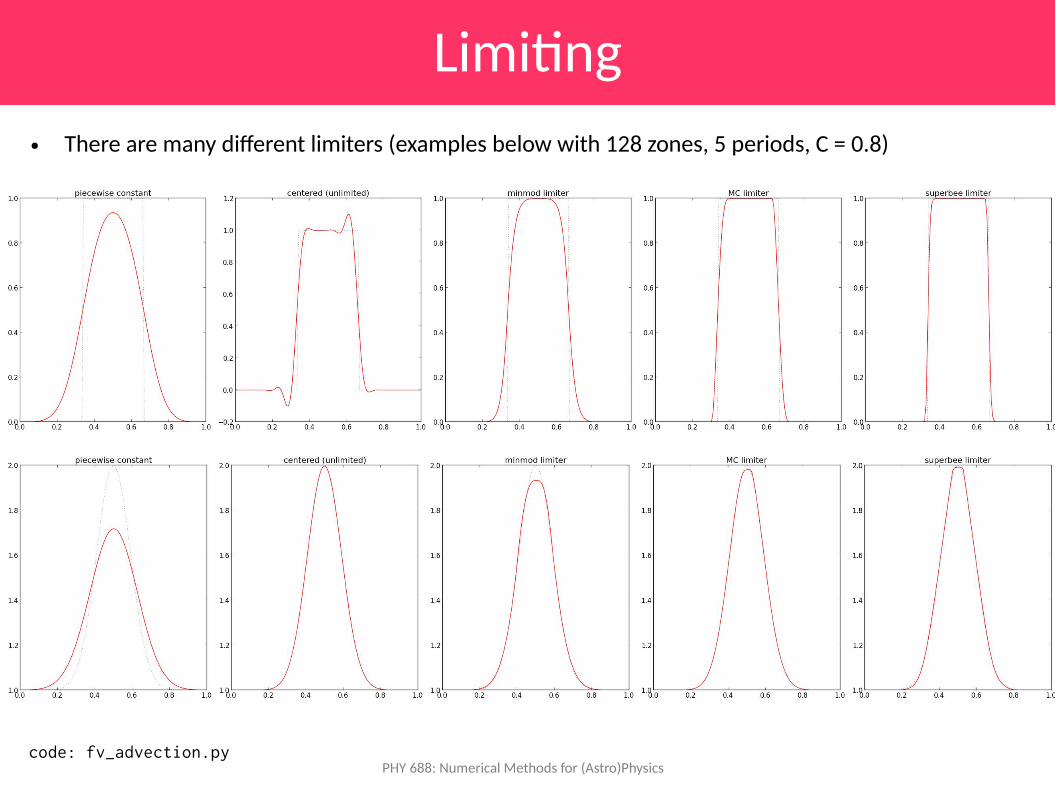
Limiting● There are many different limiters (examples below with 128 zones, 5 periods, C = 0.8)



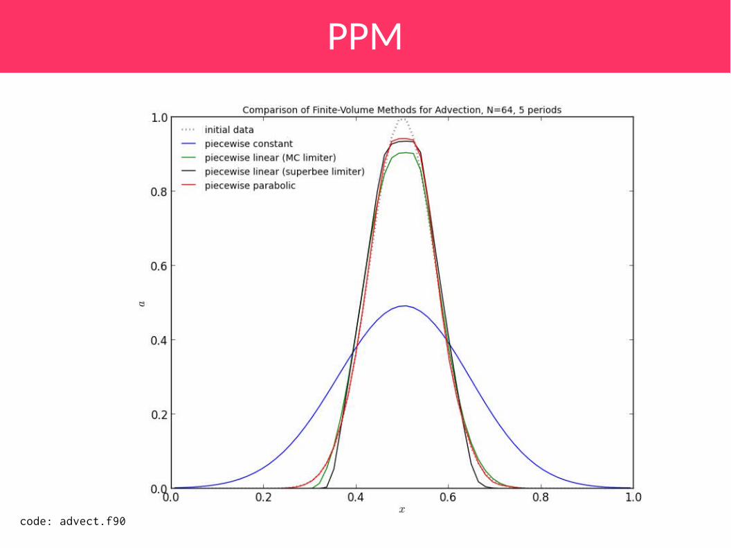
PPM● We saw that

– Piecewise constant reconstruction is first order– Piecewise linear is second order in space and time– Piecewise parabolic is the next step

● Average under parabola to find amount that can reach interface over the timestep

● In practice, the method is still second-order in time because of the centering of the fluxes, but has less dissipation

● Limiting process described in Colella & Woodward (1984)


PPM

Piecewise constant

Piecewise linear (dotted are unlimited slopes)

Piecewise parabolic (dotted are unlimited parabola)


PPM

code: advect.f90


PPM

code: advect.f90


PPM

Note: this was done with limiting on, which can reduce the ideal convergence

code: advect.f90


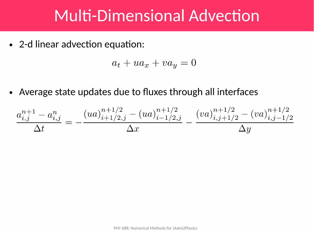
Multi-Dimensional Advection● 2-d linear advection equation:

● Average state updates due to fluxes through all interfaces


Multi-Dimensional Advection● Simplest method: dimensional splitting

– Perform the update one dimension at a time—this allows you to reuse your existing 1-d solver

● More complicated: unsplit prediction of interface states– In Taylor expansion, we now keep the transverse terms at each

interface– Difference of transverse flux terms is added to normal states– Better preserves symmetries– See Colella (1990) and PDF notes on course page for overview


Multi-Dimensional Advection

323 gaussian advected with unsplit reconstruction and C = 0.8code: https://github.com/zingale/pyro2


Burger's Equation● Recall that for the advection equation, the solution is unchanged

along lines x – ut = constant – These were called the characteristic curves

x

t

Initial point, x0

Characteristic curve, x = x0 + ût


Burger's Equation● Consider the following nonlinear hyperbolic PDE:

– This is the (inviscid) Burger's equation– We can use this as a model of the nonlinear term in the momentum

equation of hydrodynamics– The nonlinearity admits nonlinear waves like shocks and rarefactions

● Again, the characteristic curves are given as: dx/dt = u – But now u varies throughout the domain


Shocks● Shocks form when the characteristics intersect (see Toro Ch. 2 for a nice discussion)

– Solution is to put a shock at the intersection


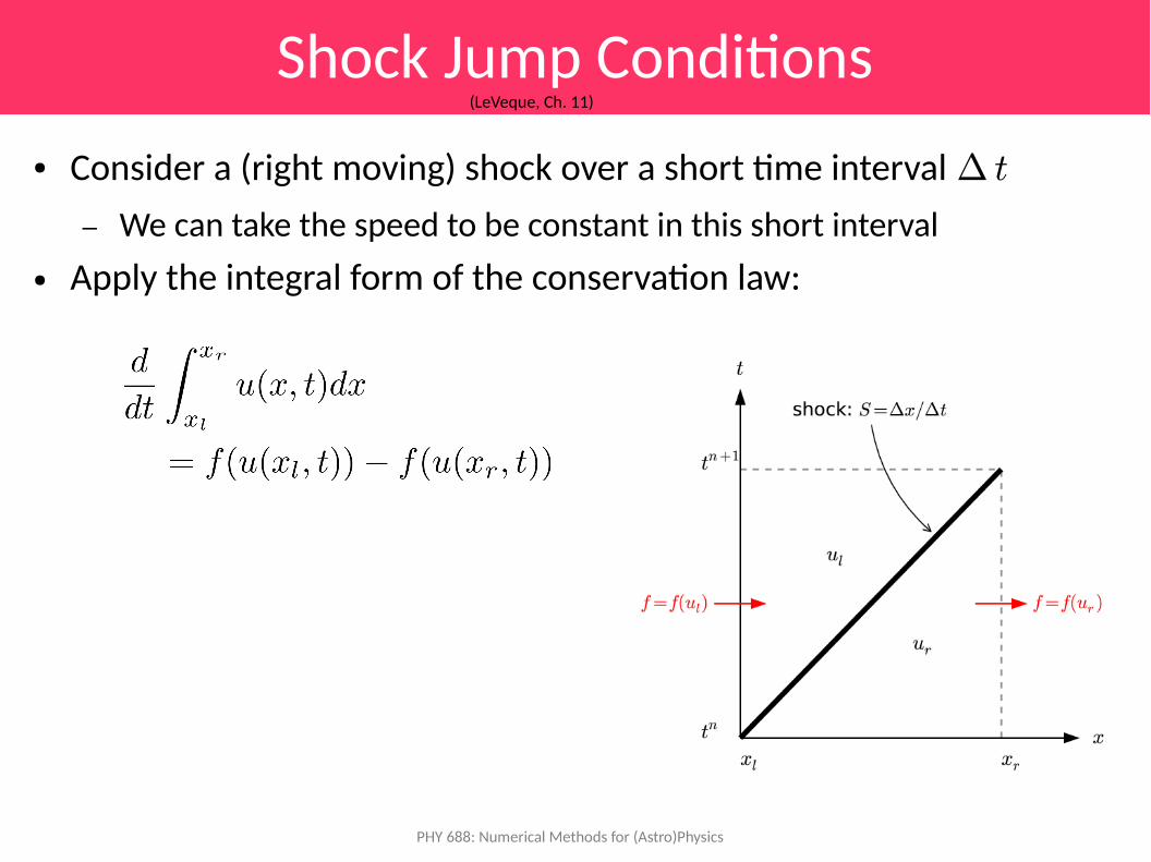
Shock Jump Conditions● Consider a (right moving) shock over a short time interval ¢ t

– We can take the speed to be constant in this short interval● Apply the integral form of the conservation law:

(LeVeque, Ch. 11)


Shock Jump Conditions● Integrating over time, we have:

– If the intervals are small, then u is roughly constant

– Taking s ≈ Δx/Δt

(LeVeque, Ch. 11)

For Burger's Eq.

This is called the Rankine-Hugoniot condition


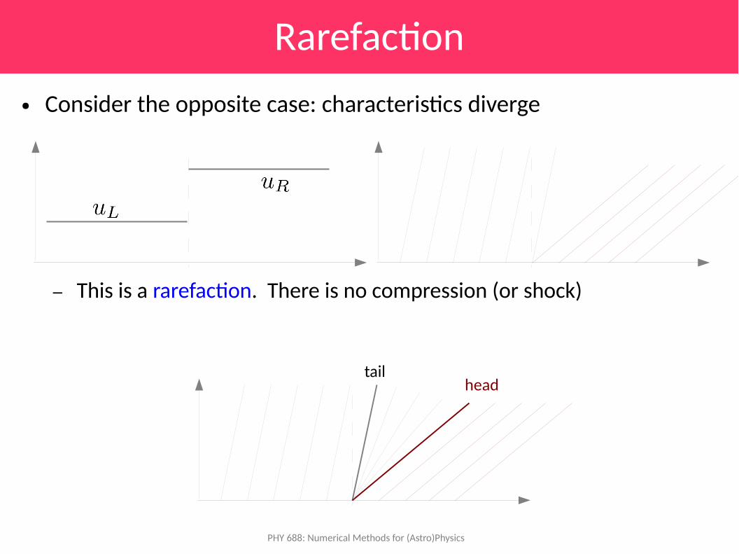
Rarefaction● Consider the opposite case: characteristics diverge

– This is a rarefaction. There is no compression (or shock)

tailhead


Burger's Equation Riemann Problem● Together, these allow us to write down the Riemann solution for

Burger's equation– We only need the solution exactly on the interface between zones– If ul > ur then we are compressing (shock):

– Otherwise: rarefaction:


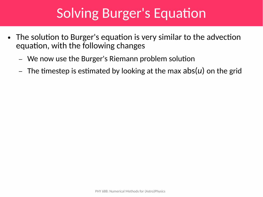
Solving Burger's Equation● The solution to Burger's equation is very similar to the advection

equation, with the following changes– We now use the Burger's Riemann problem solution– The timestep is estimated by looking at the max abs(u) on the grid


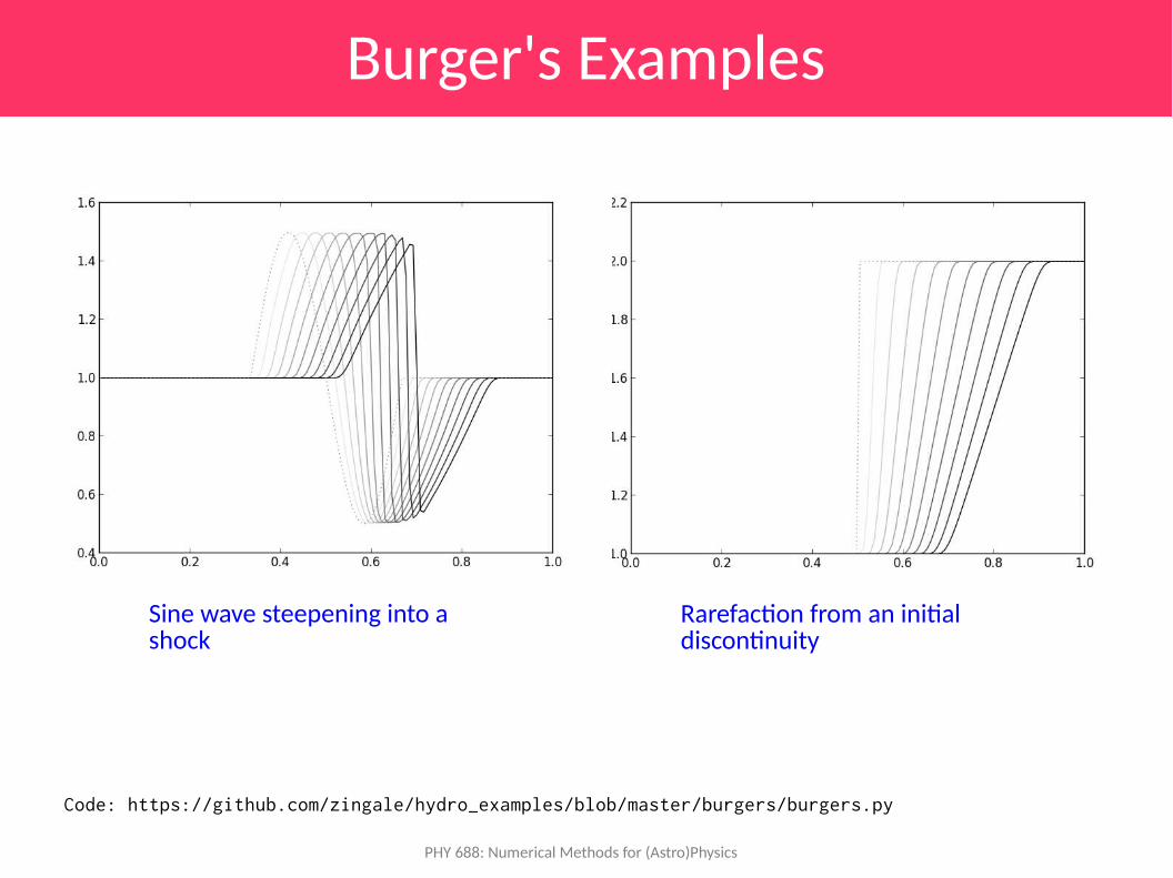
Burger's Examples

Sine wave steepening into a shock

Rarefaction from an initial discontinuity

Code: https://github.com/zingale/hydro_examples/blob/master/burgers/burgers.py


Hydrodynamics● The equations of hydrodynamics share similar ideas

– Now there are 3 waves (and three equations). We need to consider waves moving in either direction

– Shocks and rarefactions are still present– The system is nonlinear

Date post:	12-Apr-2018
Category:	Documents
Upload:	dangcong
View:	231 times
Download:	4 times

Advection / Hyperbolic PDEs - Stony Brook...

Documents