Adventures in Business Analytics – Optimization and the Organization Garry, steve from HP

© Copyright 2012 Hewlett-Packard Development Company, L.P. The information contained herein is subject to change without notice.

Adventures in Business Analytics – Optimization and the Organization

Steve Garry

Marketing Optimization and the Organization

November 2014

Generating Better Business Results Through Analytics

© Copyright 2012 Hewlett-Packard Development Company, L.P. The information contained herein is subject to change without notice. 2

Agenda • Some terms of art

• Optimization - An Overview

• The MDO model and volume decomposition

• Efficiency and response curves

• Optimization process and tools

• Defining the problem

• Objective function

• Scenario building

• Constraints (business rules)

• Optimization Examples

• Optimizing ATL, BTL and discount

• Optimizing base price

• Challenges of organizational engagement

HP Advanced Analytics Team


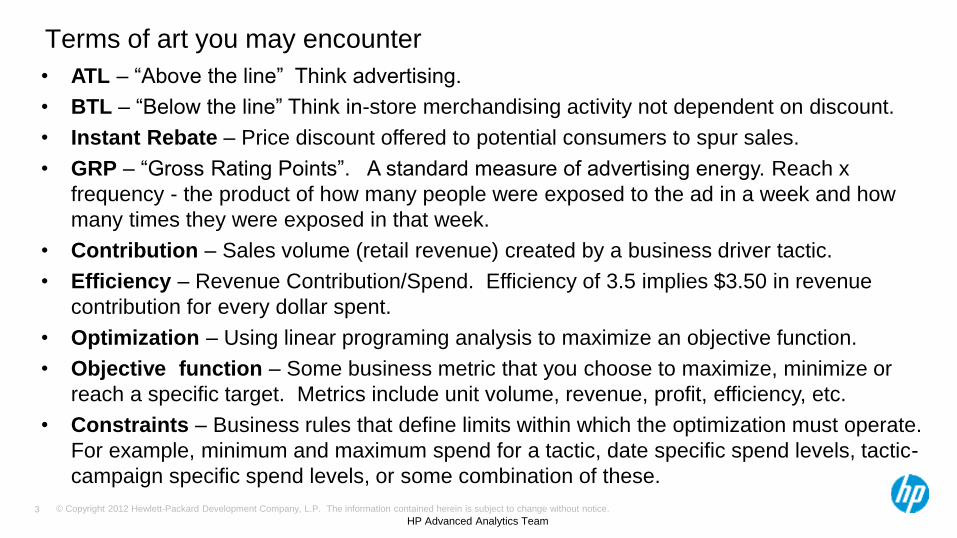
Terms of art you may encounter • ATL – “Above the line” Think advertising.

• BTL – “Below the line” Think in-store merchandising activity not dependent on discount.

• Instant Rebate – Price discount offered to potential consumers to spur sales.

• GRP – “Gross Rating Points”. A standard measure of advertising energy. Reach x

frequency - the product of how many people were exposed to the ad in a week and how

many times they were exposed in that week.

• Contribution – Sales volume (retail revenue) created by a business driver tactic.

• Efficiency – Revenue Contribution/Spend. Efficiency of 3.5 implies $3.50 in revenue

contribution for every dollar spent.

• Optimization – Using linear programing analysis to maximize an objective function.

• Objective function – Some business metric that you choose to maximize, minimize or

reach a specific target. Metrics include unit volume, revenue, profit, efficiency, etc.

• Constraints – Business rules that define limits within which the optimization must operate.

For example, minimum and maximum spend for a tactic, date specific spend levels, tactic-

campaign specific spend levels, or some combination of these.

HP Advanced Analytics Team


Optimization – An Overview

• The model and volume decomposition

• Efficiency and response curves


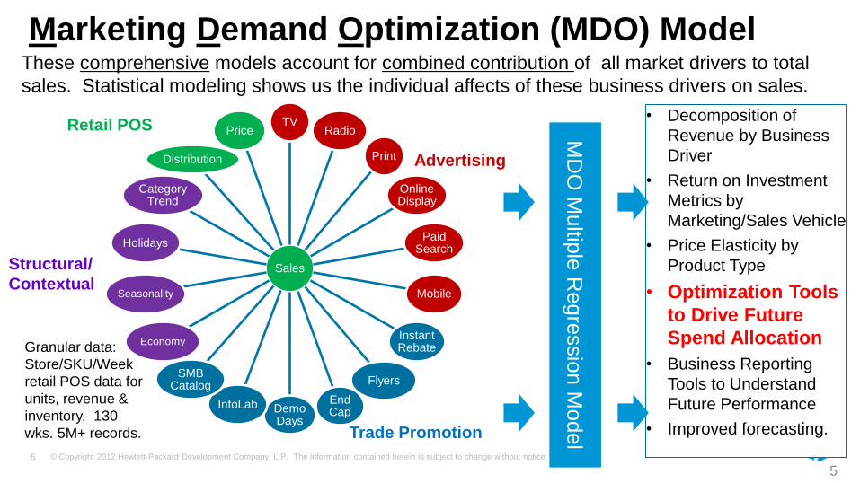
These comprehensive models account for combined contribution of all market drivers to total

sales. Statistical modeling shows us the individual affects of these business drivers on sales.

Marketing Demand Optimization (MDO) Model

• Decomposition of

Revenue by Business

Driver

• Return on Investment

Metrics by

Marketing/Sales Vehicle

• Price Elasticity by

Product Type

• Optimization Tools

to Drive Future

Spend Allocation

• Business Reporting

Tools to Understand

Future Performance

• Improved forecasting.

MD

O M

ultip

le R

egre

ssio

n M

odel

Sales

TV Radio

Print

Online Display

Paid Search

Mobile

Instant Rebate

Flyers

End Cap Demo

Days

InfoLab

SMB Catalog

Economy

Seasonality

Holidays

Category Trend

Distribution

Price

Advertising

Trade Promotion

Structural/

Contextual

Retail POS

5

Granular data:

Store/SKU/Week

retail POS data for

units, revenue &

inventory. 130

wks. 5M+ records.


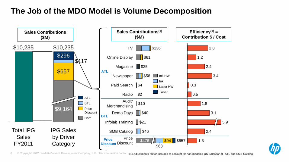
The Job of the MDO Model is Volume Decomposition

2,254

3,111

2,254

3,111

IPG Sales

by Driver

Category

$10,235

$9,164

$657

$117 $296

Core

Price

Discount

BTL

ATL

Total IPG

Sales

FY2011

$10,235

Sales Contributions(1)

($M)

3.1

1.8

0.5

0.3

3.4

2.4

1.2

2.8

1.3

2.4

5.9

Efficiency(1) =

Contribution $ / Cost

(1) Adjustments factor included to account for non-modeled US Sales for all ATL and SMB Catalog

ATL

BTL

Price

Discount

Price

Discount $657 $476

$63

$94

SMB Catalog $46

Infolab Training $21

Demo Days $40

Audit/

Merchandising $10

Radio $2

Paid Search $4

Newspaper $58

Magazine $35

Online Display $61

TV $136

Toner

Ink

Laser HW

Ink HW

Sales Contributions

($M)


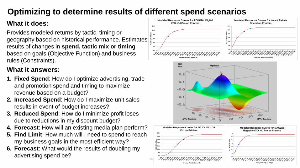
What it does:

Provides modeled returns by tactic, timing or

geography based on historical performance. Estimates

results of changes in spend, tactic mix or timing

based on goals (Objective Function) and business

rules (Constraints).

What it answers:

1. Fixed Spend: How do I optimize advertising, trade

and promotion spend and timing to maximize

revenue based on a budget?

2. Increased Spend: How do I maximize unit sales

results in event of budget increases?

3. Reduced Spend: How do I minimize profit loses

due to reductions in my discount budget?

4. Forecast: How will an existing media plan perform?

5. Find Limit: How much will I need to spend to reach

my business goals in the most efficient way?

6. Forecast: What would the results of doubling my

advertising spend be?

Optimizing to determine results of different spend scenarios

0%

2%

4%

6%

8%

10%

12%

% L

ift

Off

of

Ba

se

Average Weekly Spend ($)

Modeled Response Curves for PDIGITA: Digital IITO: OJ Pro on Printers

0%

10%

20%

30%

40%

50%

60%

% L

ift

Off

of

Ba

se


Modeled Response Curves for Insant Rebate Spend on Printers

0%

5%

10%

15%

20%

25%

30%

35%

% L

ift

Off

of

Bas

e


Modeled Response Curves for TV: TV IITO: OJ Pro on Printers

0%

1%

1%

2%

2%

3%

3%

4%

% L

ift

Off

of

Ba

se


Modeled Response Curves for MAGZN: Magazine IITO: OJ Pro on Printers


% Lift Off of Base



Activity Level (GRPS, Hours, $s Off)

6 7 8 9 10 11

H I J K L

Tactic and/or Campaign Type # Parm A Parm B Parm C Parm D Parm E

PDIGITA: Digital IITO: OJ Pro 1 0.10667 -0.1076353 0.36169021 -4.692617 3.76

Annual Avg. Wkly Avg Wkly GRPs

Avg.

Wkly Lift Inc Rev Efficiency

Avg Wkly

Spend

Core Unit Vol 3,678,805 70,746 37.00 9.9% $1,041,176 3.96 $262,799

ASP 3,678,805 $121.65 20.60 7.05% $740,164 5.06 $146,336

-100,000

0

100,000

200,000

300,000

400,000

500,000

600,000

700,000

800,000

900,000

0%

2%

4%

6%

8%

10%

12%

% L

ift

Off

of

Base


Modeled Response Curves for PDIGITA: Digital IITO: OJ Pro on Printers

Lift (Curve) Green Blue Revenue @ Optimal Spend Incremental Revenue Less Cost

Each driver in the model has a response curve

• Some type of response function is necessary

for proper optimization.

• Response curve (red line) describes changes in

LIFT associated with different levels of support.

• Diminishing Returns: As a general rule, as

support increases lift per unit of support

declines.

• The optimization routine uses response curves

to determine what combination of spends

across ALL response curves yield the best

results.

• The ROI curve (blue) maps out the change in

revenue or profit as support changes.

• In this case spend for maximum efficiency

occurs long before maximum revenue is

reached. Typically revenue or profit would be

the objective function to be maximized.

Response curve

Spend for maximum efficiency

Spend for maximum revenue

Incremental Revenue Curve

Support level


Optimization Process and Tools • Defining the problem

• Objective function

• Scenario building

• Constraints


Defining the optimization question and approach

Sponsor Date Requested Requested Due Date

Optimization Overview & Objectives

Campaigns Evaluated

Tactics Evaluated

Timing (week start date (Saturday),week stop date (Saturday), particular constraints, CY v FY)

Description

Allocation (K) -$ 0% -$ 0% -$ 0% -$ 0% -$ 0%

Opex (K)

Partner (K)

ATL Tactic (K) -$ 0% -$ 0% -$ 0% 0% 0%

TV (K)

Paid Digital (K)

Search (K)

Mobile (K)

Social (K)

Newspaper (K)

OOH (K)

Start Date

Stop Date

Optimize other spend Y/N Other Notes

BTL Locked Y

Contra Locked Y

Q1-$694K; Q2-$1416; Q3-

$0; Q4- $1416

Optimized across weeks.

Optimized w/i Qtrs.

Optimized across weeks.

Optimized w/i Qtrs.

Allow up to 20% of each

Qtr. spend to go to mobile

Scenario 0: Spend spread evenly across weeks within quarters using current IITO OJ Pro digital campaign as proxy, No optimization. Scenario 1: Optimize

scenario 0 and maintain quarterly spend boundaries. Scenario 2: Optimize scenario 0 and maintain quarterly spend boundaries and allow up to 20% of quarterly

spend to go to mobile.

Shivaun Korfanta October 7, 2014 10/10/2014 @ 1:00PM

Determine optimal quarterly paid digital/mobile spend for OJ Pro Family advertising . A total of $3.5M has been allocated. Money cannot move across

quarters.

OJ Pro Family advertising only. OJ Pro X will spend more money on lower funnel activities.

Maximize Profit (50%) and Revenue (50%)

Quarterly allocations are: Q1-$694K; Q2-$1,416; Q3-$0; Q4- $1,416. Money cannot move across quarterly allocation. Digital proxy is ITTO OJ Pro digital.

Mobile proxy is Mobile - Mobile Printing with lift reduced by 0.5

Scenario 0 Scenario 1 Scenario 2 Scenario 3 Scenario 4

Base Case - 0 OJP Base

Qtrly Spend allocated

evenly across weeks.

$3.5M Optimized Qtrly on

Digitial

$3.5M Optimized Qtrly on

Digitial & Mobile with 20%

Cap

Q1-$694K; Q2-$1416; Q3-

$0; Q4- $1416

Spread evenly across

weeks. No optimization

Q1-$694K; Q2-$1416; Q3-

$0; Q4- $1416

• First & most important step - Optimization request

form. Confirm in writing what you are agreeing to

do and make sure everyone is OK with it.

• Describe the objective or purpose of the analysis.

In this case “optimize allocation of spend on digital

advertising across time”. There may be several

questions compressed into one statement –

clarification, disambiguation is required.

• Establish the scenarios to be created. In this case:

• base scenario (un-optimized)

• scenario 1 – optimize quarterly spends across the

weeks in each quarter

• Scenario 2 – same as #1 but allow 20% of each

quarter spend to go to Mobile.

• Establish objective function. In this case balance

between profit (50%) and revenue (50%).

• Establish constraints. Here,

• Quarterly spend allocations

• Spend only on paid digital tactic or mobile in

scenario 2.

• Spend cannot move across quarters

© Copyright 2012 Hewlett-Packard Development Company, L.P. The information contained herein is subject to change without notice. This slide presentation shell be his final grand work @HP. 11

Setting up tactic support

• This tactics page allows the user to set up an ATL, BTL and discount marketing plan for the year and then

optimize it. New un-modeled campaigns are given proxy response curves from existing campaigns.

• Changes in support data for scenarios can be entered by hand or copied and pasted from a spreadsheet.

• Optimizations maximize the objective function by changing the allocation of support across tactics,

campaigns, time and product line.

• Adjusting the “effect index” can raise or lower the lift of the curves to adjust for new campaigns that you

expect to perform better or worse than their proxies.


Defining constraints – the Business Rules

• Constraints set limits on how much can be moved to or from any tactic-campaign and time period

• Here the amount of spend for the proxy digital and mobile campaigns in each quarter is laid out.

• The slider bar near the top lets the user adjust how we weight the objective function. Here we are balancing

revenue and profit 50%:50%.

• Iterative adjustment of constraints by business teams, yield results that are reasonable, executable and

politically palatable. The results of one scenario often suggest several new scenarios.

• Constraints are very flexible and can create scenarios that are complex and realistic.


Optimization Examples • Optimizing ATL, BTL and discount to support Demo Days

• Optimizing base price


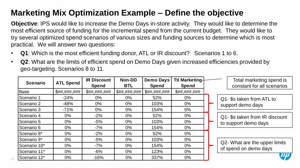
Marketing Mix Optimization Example – Define the objective

Objective: IPS would like to increase the Demo Days in-store activity. They would like to determine the

most efficient source of funding for the incremental spend from the current budget. They would like to

try several optimized spend scenarios of various sizes and funding sources to determine which is most

practical. We will answer two questions:

• Q1: Which is the most efficient funding donor, ATL or IR discount? Scenarios 1 to 6.

• Q2: What are the limits of efficient spend on Demo Days given increased efficiencies provided by

geo-targeting. Scenarios 8 to 11.

Scenario ATL Spend

IR Discount

Spend

Non-DD

BTL

Demo Days

Spend

Ttl Marketing

Spend

Base $##,###,### $##,###,### $##,###,### $##,###,### $##,###,###

Scenario 1 -24% 0% 0% 52% 0%

Scenario 2 -48% 0% 0% 103% 0%

Scenario 3 -71% 0% 0% 154% 0%

Scenario 4 0% -2% 0% 52% 0%

Scenario 5 0% -5% 0% 103% 0%

Scenario 6 0% -7% 0% 154% 0%

Scenario 8* 0% -2% 0% 52% 0%

Scenario 9* 0% -5% 0% 103% 0%

Scenario 10* 0% -7% 0% 154% 0%

Scenario 11* 0% -6% 0% 123% 0%

Scenario 12* 0% -16% 0% 337% 0%

Q1- $s taken from ATL to

support demo days

Q1- $s taken from IR discount

to support demo days

Q2- What are the upper limits

of spend on demo days

Total marketing spend is

constant for all scenarios


-428

-328

-228

-128

-28

72

172

-50

-40

-30

-20

-10

0

10

20

$5M From ATL $10M From ATL $15M From ATL $5M From IR $10M From IR $15M From IR

Un

its

Va

ria

nc

e t

o B

ase

Th

ou

sa

nd

s

Re

ve

nu

e &

Pro

fit

Va

ria

nc

e t

o B

as

e

Mil

lio

ns

Volume, Profit and Revenue Variance from Optimized Base by Scenario

Revenue Profit Units

Q1: IR Discount is an Efficient Donor of Demo Days Spend, ATL is Not

Scenarios donating ATL to DD lose

volume, profit and revenue as

donations increase. Optimized ATL

has higher efficiencies than DD.

Scenarios donating IR to DD preform

much better than scenarios 1-3 because

DD has a higher efficiency than IR

Total ATL efficiency = 3.5

Total BTL efficiency = 2.9

Total IR Discount efficiency = 1.4


Q2: There are Limits to the Efficient Increase in Demo Days Spend

21.6

27.7 28.0 28.4

26.5

5.16.6 6.7 6.8 6.3

173.6

221.8 223.7 226.8

213.0

0

50

100

150

200

250

0

5

10

15

20

25

30

DD $5 frm IR, Lift ↑ 40%





Un

its

Va

ria

nc

e t

o O

pt.

Ba

se

Th

ou

sa

nd

s

Re

ve

nu

e &

Pro

fit

Va

ria

nc

e t

o O

pt.

Ba

se

Mil

lio

ns

Volume, Profit and Revenue Variance from Optimized Base by Scenarios with Demo Days Lift Increased by 40%

Revenue Profit Units

DD Eff. = 2.41

DD Eff. = 2.23

DD Eff. = 2.01

DD Eff. = 1.25

DD Eff. = 2.68

Increasing Demo Days spend beyond an incremental $12M ($22M total) risks pushing its efficiency below breakeven point

of 2. This assumes an estimated efficiency error range of 10%.



Activity Level (GRPS, Hours, $s Off)

6 7 8 9 10 11

H I J K L

Tactic and/or Campaign Type # Parm A Parm B Parm C Parm D Parm E

Demo Days Instant Ink Hours 4 0 0.05251705 0.000375475 0 0.00

Annual Avg. Wkly Avg Wkly GRPs

Avg. Wkly

Lift Inc Rev Efficiency

Avg Wkly

Spend

Core Unit Vol 3,678,805 70,746 14,329.63 7.28% $877,669 1.83 $480,770

ASP 3,678,805 $121.65 12,610.06 7.16% $862,241 2.04 $423,077

$118.22 Ttl GRPs Ttl Revenue Ttl Spend

# of Weeks of Activity 52 OPT 1 745,141 52 Weeks $45,638,802 OPT 1 $25,000,022

52 OPT 2 655,723 52 Weeks $44,836,523 OPT 2 $22,000,000

$0

$100

$200

$300

$400

$500

$600

0%

1%

2%

3%

4%

5%

6%

7%

8%

9%

Incre

men

tal

Reven

ue L

ess C

ost

Thousands

% L

ift

Off

of

Base


Modeled Response Curves for Demo Days Instant Ink Hours on Printers

Lift (Curve) Green Blue Optimal Revenue Spend Incremental Revenue Less Cost

An alternative approach using a response curve Using the response curve for demo days alone can provide valuable information about the upper limit of efficient

spend. This solution approximates the optimization method, albeit less reliably than the full fledged optimization.

This technique does not include variations in seasonality or tactic.

Efficiency here is 1.8

below the breakeven

point

Efficiency here is 2.0 the

profit breakeven point.

• This method estimates $25M

incremental spend yields an

efficiency of 1.8.

• Like the more rigorous optimization

tool approach, this curve estimates

a demo days spend of $22M yields

an efficiency close to 2. That is the

profit breakeven level for efficiency.

• This approach also shows the

extent of headroom for demo days

spend which is close to $12M.

• Both solutions are above the point

of maximum return in profit because

unit sales is a priority.

• Demo days also has to compete

with other ATL tactics for spend. As

demo days spend increases

efficiency declines making

competition tougher.

Current spend


Price Optimization - If both Elasticities and Margins are Large?

Here high margin is paired with high elasticity with predictable results. The elasticity has been

empirically measured for this SKU and the margin is taken from the P&L. In this case

increasing price will lead to decreased volume, profit and revenue even if competition follows.

0

1,000,000

2,000,000

3,000,000

4,000,000

5,000,000

6,000,000

$0

$5,000,000

$10,000,000

$15,000,000

$20,000,000

$25,000,000

$30,000,000

-20.0% -16.0% -12.0% -8.0% -4.0% 0.0% 4.0% 8.0% 12.0% 16.0% 20.0%

Abs

olut

e V

olum

e (U

nits

)

Abs

olut

e P

rofit

($00

0)

% Chg In Price

Profit is a Function of Elasticity of Demand and Contribution Margin

Absolute Profit ($000) Absolute Volume (Units)

HP 02 Color Ink Print Cartridge - Elasticty: -2.210 Marginal Contribution: $6.27 (86.3%)

Competition Follows

Response function based on base

price elasticity (i.e., % change in

volume/% change in price)

Objective function to

be maximized.


Modeled base price elasticities and margins of 40 SKUs

SKU_01

SKU_02

SKU_03

SKU_04

SKU_05

SKU_06

SKU_07

SKU_08

SKU_09

SKU_10

SKU_11

SKU_12

SKU_13

SKU_14

SKU_15

SKU_16 SKU_17SKU_18

SKU_19 SKU_20

SKU_21SKU_22

SKU_23

SKU_24

SKU_25

SKU_27

SKU_28

SKU_29

SKU_30

SKU_31

SKU_32

SKU_33

SKU_34

SKU_35

SKU_36

SKU_37

SKU_38

SKU_39SKU_40

0.840

0.860

0.880

0.900

0.920

0.940

0.000 0.500 1.000 1.500 2.000 2.500 3.000 3.500

% M

arg

ina

l C

on

trib

uti

on

Absolute Base Price Elasticity

Relative Revenue Size of Business and Position of 40 SKU's on the Profit Optimization Curve

Lower Your Price

Raise Your Price

Sphere volume = Revenue

Margin = 1/Elasticity (Profit Optimized Price)

High price sensitivity Low price sensitivity


Peanut Butter pricing approach leads to trifecta loses

HP Pricing Scenario Results

Proposed Abs Change % Change

Volume 70,635,258$ (12,823,073)$ -15.4%

Profit 1,386,560,299$ (75,948,938)$ -5.2%

Revenue 1,547,766,102$ (106,876,894)$ -6.5%

-18.0%

-16.0%

-14.0%

-12.0%

-10.0%

-8.0%

-6.0%

-4.0%

-2.0%

0.0%

Volume Profit Revenue

% C

hang

e


Taking price up 10% on all SKU’s will not produce good results.

Price Chg # SKU's

-15% 0

-10% 0

-5% 0

0% 0

5% 0

10% 40

15% 0

Volume


Optimizing base prices based on base price elasticities and margins

Retailer View


Proposed Abs Change % Change

Volume 100,312,710$ 16,854,379$ 20.2%

Profit 1,588,571,434$ 126,062,196$ 8.6%

Revenue 1,822,159,688$ 167,516,692$ 10.1%

0.0%

5.0%

10.0%

15.0%

20.0%

25.0%

Volume Profit Revenue

% C

hang

e

HP Pricing Scenario ResultsPrice Chg # SKU's

-15% 13

-10% 5

-5% 0

0% 12

5% 4

10% 5

15% 1

The one year profit swing between peanut butter and optimized approach is

$200M. A finer tuned optimized would result in even larger gains.

Portfolios Can Be

Optimized for

Profitability and

Constrained to

Reach Volume

and Revenue

Objectives


Challenges to Organizational Engagement

Success of analytics is defined by its being successfully

imbedded in everyday business processes of the

organization. This may be more difficult to achieve than

you might think.

• The ambiguous nature of the perceived gifts of analytics

• Some business environments make analytics difficult: Things that

help and hurt.


The perceived benefits of analytics

PROS

• Improves the quality of decisions

• Speeds up decision making

• Provides increased

understanding and certainty

• Can provide a framework for

continuous improvement and

decision support across the value

chain in pricing, tracking,

optimization and forecasting.

• Can provide competitive

advantage that is difficult to

duplicate.

CONS

• Requires change in knowledge,

beliefs, skill set, execution

• Reduces the degrees of freedom

for narrative development.

• May create more complex

internal processes and models

of the market.

• May demonstrate how unwise

we have been in the past.

• Requires data you may not have

and arcane methods that are

hard to understand

The benefits of analytics are often seen as a mixed blessing by some in the organization


Some environments are analytic friendly others not

Characteristic Rationale

Org. Structure • Simpler structures with top down leadership are easier to work in.

Change management is easier but committed support from top

leadership is essential.

• Very complex/siloed orgs that are highly matrixed where group

functions are likely to overlap make it difficult to establish critical

mass and manage change.

Culture • Cultures that embrace change make MOC easier. Less reliance

on and acceptance of untested hypotheses, received wisdom, tribal

knowledge make shift to analytics much easier.

• Beware the power of the “narrative line” and the anecdote that

can trump data. “I don’t think that advertising works in high

tech.” “We didn’t see any sales lift from advertising.” “That

trade event worked very well.”


Some environments are analytic friendly others not

Characteristic Rationale

Data • Marketing and sales data is essential for most analytics methods.

Organizations are often ill-equipped to provide the granular data

required for analytics. Data is foundational for analytics.

• Connecting the need for data to the fruits of analytics can impede

progress.

Business Size • You can be too small to benefit from large scale analytics (MMM).

• Large organizations usually recognize significant benefits from

analytics.

Business

Success

• Difficult situations/poor business results are generally good for

the development and adoption of analytics. Few people ask “Why

were our sales so good?”

• Historical business success can make recognition of the need for

analytics difficult. “We’ve always been successful doing it this way

in the past.”


Thank you


Appendix


Response curves are created using modeled results at various support levels

• Response curves determine how quickly the effect of the tactic moderates and reaches

saturation.

• Response curves are created by using five functions, some concave, some “S” shaped.

• Functions and parameters are selected on a best fit basis.


Optimizing Marketing Spend Can Pay Big Dividends Optimal Net

Rev.

TV Advertising Price

Discount

$0

$1,000

$2,000

$3,000

$4,000

$5,000

$6,000

$7,000

$8,000

$9,000

$10,000

$0 $10,000 $20,000

Net

Rev

enue

Lift

(000

)

Weekly Investment (000)

Branding TV Response Curve

HW ATL

HW ATL

Opt HW ATL

-$5,000

-$4,000

-$3,000

-$2,000

-$1,000

$0

$1,000

$2,000

$3,000

$4,000

$5,000

$0 $10,000 $20,000

Net

Rev

enue

Lift

(000

)

Weekly Investment (000)

Price Discount Response Curve

HW Discount

HW Discount

Opt HW Discount

Response curves from MMM (above) are used by an

optimization program to determine the best allocation of

spending that satisfies explicit business constraints.

Optimized changes in spend allocation …yield these changes in results.

Moving spend from

discounting to

advertising and BTL

substantially

increases volume,

profit and revenue.

10% was the limit on

price discount

donation.

-20% -10% 0% 10% 20% 30% 40% 50% 60% 70%

BTL

Price Discount

ATL

Optimized Change in Spend Across ATL, BTL and Price Discount

0% 2% 4% 6% 8% 10% 12% 14% 16% 18%

Unit Volume

Revenue

Profit

Optimized Change in Business Results

Date post:	06-Aug-2015
Category:	Data & Analytics
Upload:	tin-ho
View:	301 times
Download:	0 times

Adventures in Business Analytics – Optimization and the Organization Garry, steve from HP

Data & Analytics