I AECL-7254 THERMAL-HYDRAULICS IN RECIRCULATING STEAM GENERATORS THIRST Code User's Manual Model of steam generator used for analysis THIRST code results. Prufi'es of mass flux and s'eam quality CARACTERISTIQUES THERMOHYDRAULIQUES DES GENERATEURS DE VAPEUR A RECiRCULATION Manuel de I'utilisateur du code THIRST M.B. CARVER. L.N. CARLUCCI, W.W.R. INCH April 1981 avril
Transcript
IAECL-7254
THERMAL-HYDRAULICS IN RECIRCULATINGSTEAM GENERATORS
THIRST Code User's Manual
Model of steam generator used for analysis THIRST code results. Prufi'es of mass flux and s'eamquality
CARACTERISTIQUES THERMOHYDRAULIQUESDES GENERATEURS DE VAPEUR A RECiRCULATIONManuel de I'utilisateur du code THIRST
M.B. CARVER. L.N. CARLUCCI, W.W.R. INCH
April 1981 avril
ATOMIC ENERGY OF CANADA LIMITED
THERMAL-HYDRAULICS IN RECIRCULATING STEAM GENERATORS
THIRST Code User's Manual
by
M.B. Carver, L.N. Carlucci, W.W.R. Inch
Chalk River Nuclear LaboratoriesChalk River, Ontario
1981 April
AECL-7254
L'ENERGIE ATOMIQUE DU CANADA, LIMITEE
Caractéristiques thermohydrauliques des générateurs de vapeurâ recirculation
Manuel de l'utilisateur du code THIRST
par
M.B. Carver, L.N. Carlucci et W.W.R. inch
Résumé
Ce manuel décrit le code THIRST et son utilisation pourcalculer les ëcnlaments tridimensionnels en deux phases etles transferts ae chaleur dans un générateur de vapeurfonctionnant à l'état constant. Ce manuel a principalementpour but de faciliter l'application du code.S l'analyse desgénérateurs de vapeur typiques des centrales nucléaires CANDU.Son application à d'autres concepts de générateurs de vapeurfait l'objet de commentaires. On donne le détail deshypothèses employées pour formuler le modèle et pour appliquerla solution numérique.
Laboratoires nucléaires de Chalk RiverChalk River, Ontario
KOJ 1J0
Avril 1981
AECL-7254
ATOMIC ENERGY OF CANADA LIMITED
THERMAL-HYDRAULICS IN RECIRClfLATIWG STEAM GENERATORS
THIRST CODE USER'S MANUAL
by
M.B. Carver, L.N. Carlucci, W.W.R. Inch
ABSTRACT
This manual describes the THIRST code and its use in computing
three-dimensional two-phase flow and heat transfer in a steam
generator under steady state operation. The manual is intended
primarily to facilitate the application of the code to the
analysis of steam generators typical of CANDU nuclear stations.
Application to other steam generator designs is also discussed.
Details of the assumptions used to formulate the model and to
implement the numerical solution are also included.
Chalk River Nuclear LaboratoriesChalk River, Ontario
KOJ 1J01981 April
AECL-7254
(i)
TABLE OF CONTENTS
1. INTRODUCTION 1
1.1 Steam Generator Thermal-Hydraulics 21.2 The Hypothetical Prototype Steam Generator . . . . 51.3 The THIRST Standard Code and its Intended
Application 71.4 The Use of This Manual 7
2. FOUNDATIONS OF THE MODEL 9
2.1 The Governing Equations 92.2 Modelling Assumptions 112.3 Boundary Conditions 122.A Overview of the Solution Sequence . 122.5 Thermal-Hydraulic Data 16
2.5.1 Fluic1 Properties and Parameters 16
2.5.2 Empirical Relationships 17
3. IMPLEMENTATION FUNDAMENTALS 18
3.1 The Coordinate Grid 183.2 The Control Volumes 193.3 The Control Volume Integral Approach 24
3.3.1 Integration of the Source Terms 243.3.2 Integration of the Flux Terms 25
3.4 The 'Inner' Iteration 263.5 Stability of the Solution Scheme 28
3.6 Notation used in THIRST 323.7 Formulation of the Source Terms . - 33
- ii -
TABLE OF CONTENTS (continued)
Page
4. APPLICATION OF THIRST TO ANALYSE THE PROTOTYPE DESIGN . . . 34
4.1 Design Specification 354.2 Grid Selection 35
4.2.2 Baffles 364.2.3 Partition Platfi 364 . 2 . 4 Windows 384.2.5 Axial Layout (I Plane) 384.2.6 Radial Division (J Planes) 404.2.7 Circumferential Division (K Planes) 424.2.8 Final Assessment 42
4.3 Preliminary Data Specification 434.4 Preparation of the Input Data Cards 644.5 Sample Input Data Deck 654.6 The Standard Execution Deck 694.7 Job Submission 70
5. SOME FEATURES OF THE THIRST CODE 72
5.1 The RESTART Feature 725.2 The READIN Feature 755.3 Time Limit Feature 775.4 Advanced Execution Deck 78
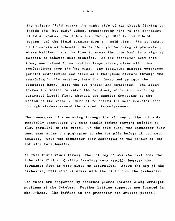
continuity- It does, however, introduce additional complexities,
as the finite difference form of each equation must be
Integrated using a control volume centered on the primary
variable concerned. Thus scalars are considered to be constant
over control volumes centered at grid points, while the axial
momentum equation is integrated over a control volume centered on
the U velocity, and the radial and azimuthal momentum equations
are centered on V and W, respectively. Typical control volumes
for each of these four cases are also shown in Figures 3.1 to
3.4.
K +1
- 20 -
K RH
K - 1
J + 1
K - J ( r - 6 ) PLANE
I x+
V(I ,J ,K)
t"-
X +
I
hU.JJQ
1 + 1
<" I.CT . M\ Iu ( I , J , K )
T
J - I K+ 1 K K - 1
I - J ( x - r ) PLANE I - K (x -9) PLANE
Figure 3.1: Clrid Layout showing Scalar and Vector Locations
- 21 -
K + 1
1
\ \
r +
r /
/ /
K -1
K) J + 1
K -J ( r -8) PLANE
R~
— —
r~
—i
/ P /
x +
—
7-r-l
ii
-f-
iii
I - 1
9
+
-
/ t
— i
X
i u(
x~
1— —
1
,J,
B
0
—1
1
I +1
i -
J - 1 J J + 1 K + 1 K K - 1
I - J ( x - r ) PLANE I -K(x - 9 ) PLANE
Figure 3.2: Control Volumes for Scalar Quantities
- 22 -
K +1K- 1
J + 1
K - J ( r ~9) PLANE
+-K)
Ir
4 - 1 - 1i
I - J (x - r ) PLflNE
I
Ir
K + 1 K
•i +
V(I ,J ,K) I
i
T~- f — 1 - 1
IK- 1
I - K ( x - 0 ) PLANE
Figure 3.3: Control Volumes for Radial Velocity Vectors
- 23 -
K + 1 K- 1
J +1
J -I
K - J (r - 8 ) PLANE
+-!•!
r -'/ W(I,J,K) |Mfv
I
J - 1 J
I -J (x - r) PLANE
I - 1
t-
+4-I-H-K + 1 K K - 1
I -K (x -6 )' PLANE
Figure 3.4: Control Volumes for Circumferential Velocitv Vectors
- 24 -
3. 3 The Control Volume Integral Approach
Although the equations to be solved are Integrated over
different control volumes, the procedure in each case Is
completely the same. Thus, each equation may be written in the
form of equation 2.1 and integrated
[7 £ I ±
-0S rdrdOdz = 0 (3.1)
Although the integration Is done formally by use of Gauss
theorem,
JJJ -<t>dv =/7"(n-<J>)ds (3.2)v JJs
the result is Intuitively obvious from first principles.
It is
r, l r II (g rpv4 i ) n - (grpvcf) I A9Az + l(Bpw<}>) - (Bpwc|>)wl ArAz
[ I rrr(6pu<( i ) , - ( 6 p u < ( ) ) . | rA<J>Az • / / / B S . d v ( 3 . 3 )
h %1 JJJ *The (quantities) obviously represent the flux through the
appropriate control volume face, and the [quantities] represent
the flux imbalance In each coordinate direction.
3.3.1 Integration of the Source Terms •
The source terms are frequently non-linear in 41 • Integration of
these terms is accomplished tsrm by term. The result can be
- 25 -
l i n e a r i z e d with respect to <b and s ta ted in general form as
S v = Su + Sp<|>p (3.4)
Here the term Sp normally contains all coefficients of (J> , and
Sy contains remaining terms which are generally (but not
always) unrelated to (|> .
Reexamining the equations in Table 2.1, it is apparent that the
greater part of the programming in the THIRST code is involved
with formulating and integrating the resistance components of
the source terms, using the appropriate empirical correlations.
This is done in subroutines with the generic name SOURC.
3.3.2 Integration of the Flux Terms
It is apparent from equation 3.3 and figure 3.2 that values at,
for example, control volume face n can be obtained to first
order accuracy by upwind approximation for any variable A, which
assumes that the velocity vector convects scalars from upwind
only. Thus if all velocities are positive, inlet flows convect
neighbouring scalars, outlet flows convect the control volume
scalar. Denoting the coefficients of <f> by C, and using the
upwind approximation, equation 3.3 is reduced to the i?orm
C <f> - C <j> + C < t > - C A = S + S < f > ( 3 . 5 )n p S3 e¥p wYw u p Y p v '
where C. is the flux evaluated at control volume face i.
_ 26 -
Collecting terms gives
i = n,s,e,w,h,£
(3.6)
A = C A = C etc.n n s s
A = £A. - SP i P
Once the coefficients A have been computed, equation 3.6 is the
standard linear equation set
A <f> =- B (3.7)
which can be readily solved
<(i - A" 1 ] ! (3.8)
Actually, the size of the matrices prohibits direct solution, so
iterative methods are used, and equation 3.8 is solved by an
'inner' iteration.
3.4 The 'Inner' Iteration
The matrices of equation (3.7) are too large to permit direct
solution of the equation set by means of (3.8) even when sparse
matrix techniques are considered, so an Iterative technique is
used. It is well known that the solution of equation sets in
which the matrix A is tridiagonal can be performed extremely
quickly as the algorithm reduces to recursive form.
- 27 -
Equation 3.7 can be converted to trldiagonal form by Including,
for example, only the coafficients along the r direction on the
left-hand side.
Vn + Vp + Vs " ~(SV.i + V(3.9)
j = e,w,5.,h
Similar expressions can be written for the 6 and z directions.
Ve + V P + Vw " "(rVj + Su}
(3.10)
j = n,s,fc,h
V h + \*P + V l " -(lAj*i + V(3.11)
j = n,s,e,w
A one-dlmenslonal problem can be solved directly by (3.9). A
two-dimensional problem Is solved by an alternating direction
Iteration ADI method. This Involves solving 3.9 and 3.10
alternately until the solutions converge. A three-dimensional
solution requires the solution of 3.11 in addition. This
creates several possibilities. For example, 3.9 and 3.10 could
be solved for a number of iterations for each time 3.11 is
solved. The most suitable strategy depends on the nature of the
flow problem. The THIRST code has a number of different
strategies designed to promote convergence in three dimensions.
These are discussed in Appendix A.
- 28 -
3. 5 Stability of the Solution Scheme
The outer iteration scheme discussed in Chapter 2 normally
proceeds to convergence in a stable manner, and converges
rapidly, providing each inner iteration is stable.
To promote stability of the iterations, three principal devices
are incorporated in THIRST. The first, that of under-relaxation,
is common to most iteration schemes. The second, upwind weighted
differencing, is frequently used to stabilize both steady state and
transient thermal-hydraulic calculations [10]. The third concerns
the formulation of the source terms to ensure stability.
.5.1 Under-Relaxation
Because the solution is obtained by iteration, there is a strong
likelihood that variable values may fluctuate unduly during the
initial stages. It is common practice to stabilize these
fluctuations using under-relaxa tion • Thus if (j)N is calculated
from 3.9 to 3.11 using previous values <j> , it is then replaced
l> - a* + ( l a H " 1 (3.12)Relax Calc. old
Relaxation factors a for each equation solution are supplied
with the THIRST code, but may be changed by data input if
necessary.
In practice, it is possible to impose under-relaxation before
attempting the linear equation solution instead of after Its
completion. This is preferable as it minimizes the chances that
the linear equation solution itself may generate unlikely
values.
- 29 -
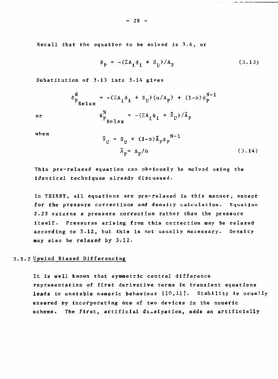
Recall that the equation to be solved is 3.6, or
(3.13)
Substitution of 3.13 into 3.14 gives
<dp = -(EA c(> + S,.)(a/A )rRelax l l u r
or *p = -(SAid)i + SRelax
when „
\ • S Nu + <Ap= Ap/a (3.14)
This pre-relaxed equation can obviously be solved using the
identical techniques already discussed.
In THIRST, all equations are pre-relaxed in this manner, except
for the pressure corrections and density calculation. Equation
2.23 returns a pressure correction rather than the pressure
itself. Pressures arising from this correction may be relaxed
according to 3.12, but this is not usually necessary. Density
may also be relaxed by 3.12.
3.5.2 Upwind Biased Differencing
It is well known that symmetric central difference
representation of first derivative terms in transient equations
leads to unstable numeric behaviour [10,11], Stability is usually
ensured by incorporating one of two devices in the numeric
scheme. The first, artificial dissipation, adds an artificially
- 30 -
large viscous term to the equations. The second, upwind
differencing uses difference formulae which are asymmetrically
weighted towards the upwind or approaching flow direction. Both
devices stabilize the computation and, in fact, it can be shown
that they are numerically equivalent [11].
Central differencing has the same destabilizing effect in steady
state, and computations can be stabilized by the same devices.
Consider, for example, a one-dimensional central difference
statement of equation 3.5.
2 - Cs 2 + S = 0 (3.15)
This can be reduced to
C'<t>r. ~ C <(>„ ~ 2 S J
As CB approaches Cn, the denominator becomes very small,
generating undue excursions in efi values. In particular if Cs
exceeds Cn very slightly, a small increase in <|>s gives a
large decrease in <);_ - an impossible situation.
However, if we add diffusion terms which involve the second
derivative, the resulting equation can be shown [13] to be
(D + C )<(>„ + (D - C )4> - 2S,, _ s s S n n TN A ,, , ,,.*P D + D + C - C ( 3 < 1 7 )
n s n s
- 31 -
Note that 3.17 will always be stable providing the diffusion
Influence Dn + Ds Is large enough.
Similarly on physical reasoning alone, one may consider that <J>
is swept primarily in the direction of flux. The simple upwind
statement of 3.16 already introduced in section 3.5 is
Cn*P " Cs*S
This r e d u c e s to
C <J> - S,t=p = - 2 - 2 * ( 3 . 1 8 )
n
which will always be stable.
Equation 3.18 is the simplest possible upwind formulation and is
equivalent to adding excess viscosity. Its use has been
criticized because it can lead to diffusion of the solution,
particularly when the flow direction is not normal to the grid
axes [14,15]- A number of higher order difference schemes which
can be used to give more accuracy may be developed [10,12] and
some of these may be implemented in schemes similar to that used
in THIRST [15].
In the THIRST code, the simple formulation is retained, however.
The large flow resistances and heat sourras due to the closely
packed tube bundles in the steam generators dominate the
computation to •rjch an extent that the differences which would
be caused by higher order methods are believed to be minor.
- 32 -
3.6 Notation used in THIRST
Finally, we have up to here been using single subscripts n, s,
etc. for simplicity. The code,however, is written in
cylindrical coordinates and uses terms such as AXM to denote
A x_. On this basis, equation 3.6 becomes
A<|> = E A < J > + S (3.19)
where:
A = A , + A + AQ, +AQ + A . + A + DIVG - SPp r+ r - 6+ 9- x+ x-
The upwind formulation can be implemented to consider flow
d i r e c t i o n au tomat ica l ly in the following manner:
r+r+2
r-2 r+
(Bpav)r+
face area
r-2
C(6pav) (3.20)
1§±2 C Q +
(@paw)0 +
etc .
t C , " mass flow through control volume face r,; depending on the
transport parameter <(>; 3> P> v ara either defined at that
face or interpolated to that face.
- 33 -
DIVG = C r + - Cr_ + C e + - Ce_ + C x + - Cx_
= net accumulation of mass in the control volume
The table below defines A^ and <P± for each i:
i „ Ai »1
A r + \ +Ar- V
6 + A 6 + *0 +
6" A9- *9-X + Ax+ *X+
x- A <(>
Note that this formulation also automatically handles possible
extreme cases In which all flow directions but one are in
towards (or out away from) a control volume.
3.7 Formulation of the Source Terms
For stability of the inner iteration, it is essential that the
coefficients remain positive after the source terms are incor-
porated. Thus, in 3.20, SP must be negative. Cases in which
SP tends to be positive are catered for by artificially2
augmenting SU . For example, if S = -KpV , one may write
SP - -2Kp|v|, SU - +KpV2; SU will then incorporate the old value
of V, and SP will ensure the formulation is both stable and
implicit.
This section completes the overall description of the model
implementation. The following chapters contain detailed instruc-
tions on how to use the code.
- 34 -
4. APPLICATION OF THIRST TO ANALYSE THE PROTOTYPE DESIGN
Specification of the three-dimensional model must include
details of all relevant geometrical, fluid flow and heat
transfer parameters. It is emphasized that the process of
modelling a steam generator relieF heavily on diligent assembly
of the specifications, optimal choice of grid layout, and of
course correct preparation of the input data. This chapter is
intended to guide the user step by step through the considerable
effort required.
By means of a detailed example, we illustrate the entire
procedure required to prepare a THIRST analysis of a particular
steam generator design. We assume the user is familiar with the
fundamentals discussed in Chapters 2 and 3, and now discuss
Design Specification - the hypothetical steam generator
Grid Selection - arrangement of optimal grid layout
Preliminary Data Specification - procedure for assembling
the data specification sheets
Preparation of Input Data Cards
Sample Input Deck
Execution Deck - assembly of a THIRST job and submission
to the C£C computer
- 35 -
4. x Design Specification
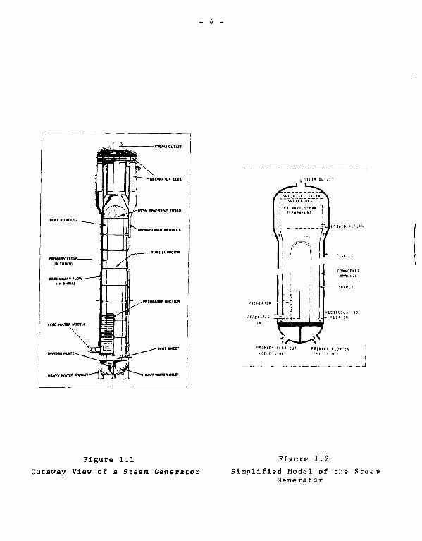
The particular case chosen for this example is the hypothetical
steam generator discussed in Chapter 1 and shown in Figure 1.2.
Design parameters used in the current example are summarized In
Table 1.2.
A large number of variations of this design can be investigated
using the standard THIRST code by specifying parameter
variation through input data.
Designs which deviate from the hypothetical model in major
aspects may require code modifications. These are considered in
Chapter 5.
4,2 Grid Selection
The first task is to describe the geometry of the design to the
computer. This is accomplished by superimposing a cylindrical
coordinate grid onto the design, and by specifying the location
of flow obstacles in terms of this grid. THIRST accepts a
maximum of 40 axial planes, 20 radial planes and 20
circumferential planes; however,due to a storage limitation, the
maximum number of nodes must not exceed 4900.
In order to appreciate the selection of grid locations, the user
should understand the staggered grid arrangement used in THIRST
described in Chapter 3. Essentially, velocities are centered
between gri<1 lines in their corresponding direction and centered
on grid lines in the other two directions, as shown in Figure 3.1
An axial velocity, for example, has a control element with
- 36 -
boundaries as shown In Figure 3.2. The cop boundary corresponds
to the I plane, the bottom to the 1-1 plane. The left side
boundary is located midway between the J and J-l planes. The
radial velocity has a control element that extends between J
planes and straddles I and K planes. And similarly, the
circumferential velocity extends between K-planes and straddles
the I and J planes.
4.2.2 Baffles
Figure 4.1 shows how the code handles flow around a typical
baffle. We observe a radial flow to the left under the baffle,
an axial flow around the baffle followed by a radial flow to the
right above the baffle. Note that the baffle lies in the middle
of the U velocity control element and the radial control
elements lie on either side of the baffle. We can see that
axial grid lines must be located such that the baffle plates lie
midway oatween them.
4.2.3 Partition Plate
Figure 4.1 also shows the code treatment of the partition plate.
The circumferential velocity W corresponding to the K plane is
blocked by this partition plate which is centered between the K
and K-l planes.
- 37 -
J +2 J +1 J - t
-example of avelocity blocked bythe baffle
TYPICAL BflFFLE^
SHROUD
"(I+1,J,K) -carries the| + | flow out radially
U(1+1,J-1,K) -carriesthe flow un past thebaffle
V(I,J,K) -carries theflow in radially
Pf lRTITION PLATE
The I-planes are located so that baffles lie midway between them. Thelocation of the J-planes matches the baffle cuts for this particularK-plane; however, the cut will not match other K-planes and the programis set up to handle this.
Figure 4 . 1 : Grid Layout at a Baffle P la te
SHELL
-downcomer velocity
-shroud windowvelocity
SHROUDJ + 2 J - I
-velocity insideshroud
TU BESHEET
The I and 1-1 planes are located so that the top of the window lieshalfway between them. The J+l and J+2 planes center the shroud.Generally, more grid would be located in the shroud window to handlethe sudden change in flow direction.
Figure 4.2: Grid Layout at a Shroud Window
- 38 -
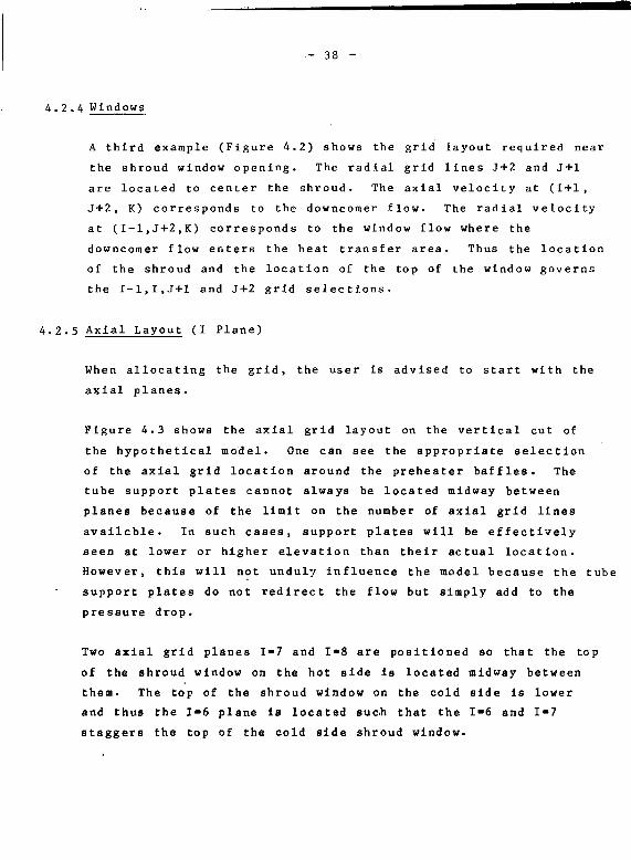
4.2.4 Windows
A third example (Figure 4.2) shows the grid layout required near
the shroud window opening. The radial grid lines J+2 and J+l
are located to center the shroud. The axial velocity at (1+1,
J+2, K) corresponds to the downcomer flow. The radial velocity
at (I-1,J+2,K) corresponds to the window flow where the
downcomer flow enters the heat transfer area. Thus the location
of the shroud and the location of the top of the window governs
the 1-1,1,J+l and J+2 grid selections.
4.2.5 Axial Layout (I Plane)
When allocating the grid, the user is advised to start with the
axial planes.
Figure 4.3 shows the axial grid layout on the vertical cut of
the hypothetical model. One can see the appropriate selection
of the axial grid location around the preheater baffles. The
tube support plates cannot always be located midway between
planes because of the limit on the number of axial grid lines
available. In such cases, support plates will be effectively
seen at lower or higher elevation than their actual location.
However, this will not unduly influence the model because the tube
support plates do not redirect the flow but simply add to the
pressure drop.
Two axial grid planes 1-7 and I«8 are positioned so that the top
of the shroud window on the hot side is located midway between
them. The top of the shroud window on the cold side is lower
and thus the 1-6 plane is located such that the 1-6 and 1-7
staggers the top of the cold side shroud window.
- 39 -
PXIOL GRID LRYOUT
BUNXE
SHROUD-
SHELL-
TUBESUPPORT-
PLOTE
PREHERTEROBFTTJE-
PLBTE
FEEDURTERINLET
SHROUD-WINDOW
1-T TI IJ.L.
TfJ-L
rr1L
-H-
D J
- Ir
±£
35,3634
33
32
COLD SIDE HOT SIDE
31
30
29
28
27
26
25
24
23
21,2220
19
18
17
16
15
14
13
1210,118,96,74,51-1,2,3
Figure 4 .3 : Axial Grid Layout
- 40 -
When the axial planes have been allocated to satisfy the axial
flow obstacles such as baffles, tube support plates, window
openings, etc., the user should then examine areas which are
critical to the analysis and ensure that a sufficient number of
grid planes are located in these areas. For instance, the
region just above the tubesheet at the shroud window is
particularly important. The 1=2 plane is located just above the
tubesheet. The 1=3 to 1=5 are added to this region to provide
more detail. The 1=22 plane is added above the preheater to
handle the migration of hot side flow to the cold side.
To enable the tracing routine used to calculate the heat
transfer in the U-bend, an axial plane must be located at the
start of the U-bend curvature. At least 3 additional axial
planes should be located in the U-bend to ensure the accuracy of
the routine which calculates the pressure drop and heat transfer
in the U-bend. linally the last plane should be located very
close to the second last plane so that the axial boundary values
which are based on the last Internal values can be calculated.
4.2.6 Radial Division (J Planes)
In our example, we have used 36 axial planes. We have now
4900/36 » 136 more nodes available to share between the radial
and circumferential directions. Figure 4.4 shows a horizontal
cross-sectional cut of our design. Note that only one half of
the steam generator is modelled as the design is symmetric about
a line dividing the hot and cold sides. The bundle boundaries
and baffle plate edges are marked as dashed lines. The shroud
and shell locations are shown as solid lines.
RRDIPL OND CIRCUriFERENTIRL GRIDK-7 K-6
K-B
K-9
FEEDUPTERBUP3LE
K-tO
K-n
K-123 4 5 6 7 B 9 10
SHELL
DOWNCOMERPNNULUS
SHROUD
TUBEBUNDLE
I
K-2
K-l
PREHEPTER BRFFLEPLRTE EDGE
Figure 4.4: Radial and Circumferential Grid
- 42 -
Figure 4.4 also shows the radial grid layout. J=l corresponds
to the center point. The second radial position, J=2, is located
very close to the J=l point because it is the first active point
in the radial grid pattern. The J=9 and J=10 points are located
so as to center the shroud inner radius, as discussed
previously. The J=3 to J=8 points are positioned at equal
intervals as specific locations are not dictated by special
geometrical features.
4.2.7 Circumferential Division (K Planes)
We have now used 36 x 10 = 360 grid planes and we have
4900/360 ~ 13 grid planes left to be allocated in the circumfer-
ential direction. To simplify the layout, we will only use 12,
with equal numbers on the hot and cold side. The code can
accept unequal numbers of grid planes on the cold and hot side
if the geometry requires it. The K=6 and K=7 planes are located
such that they straddle the partition plate. The K=2 and K=ll
planes, the first and last internal planes are located fairly
close to the boundary points as they are the first active points
inside the boundary. The remaining points are spaced equally;
however, this is not a requirement, and spacing may be adjusted
to fit particular geometrical features.
A.2.8 Final Assessment
This then completes the grid layout. One may find that the
number of planes in each direction could be juggled to better
model the design. Once the grid layout has been finalized and
the geometry of the design described to the code relative to
- 43 -
this grid, It is a major undertaking to alter the grid location.
Thus it is important at this stage to review the grid selection
carefully.
Preliminary Data Specification
Having examined the design layout and selected the optimum
grid location, we must now provide the code with the information
required to model the design. This section describes the
contents of data sheets. The specification sheets are included
In chart form to emphasize that specification must be completed
and verified before any actual input data cards are prepared.
Each chart Is divided into the following columns:
COLUMN 1: DATA SO. - for reference purposes
COLUMN 2: DESCRIPTION
COLUMN 3: DATA VALUES - to be taken from specifications
COLUMN 4: REMARKS - any manipulation of the DATA isdescribed or a summary of optionsis given
COLUMN 5: VARIABLE NAME - code name used in THIRST
COLUMN 6: FINAL VALUE - value to be used as data
The data is arranged in functional groups as follows:
GROUP 1: Preliminary Data (Items 1 - 7 )
GROUP 2: Geometric Data Entered by Grid Indices(Items 8 - 21)
GROUP 3: Geometric Data Entered by Value(Items 22 - 41)
GROUP 4: Correlations and Resistances (Items .42 - 60)
GROUP 5: Operating Conditions (Items 61 - 69)
GROUP 6: Utility Features (Items 70 - 85)
Items within each group are arranged alphabetically for ready
reference.
DATANo. DESCRIPTION
DATAVALUE REMARKS VARIABLE
NAME VALUE
ITEMS 1 - 7 PRELIMINARY DATA
1
2
3
4
5
6
7
Controls the use of the restartption (see Section 5.1)
Nuaber of axial planes
Hiwber of radial planes
Nmfcer of circumferential planes
Location of axial planes
Location of radial planes
Location of circumferential gridplanes
—
—
—
—
—
—
RESTART " 1.0 - new run, no RESTART tape usedas input
RESTART = 2.0 - continue executing from apoint reached in a previousrun
RESTART = 3.0 - attach the data stored on tapefrom a previous run and printand/or plot the data
RESTART = -(1 or 2 or 3) - proceed as abovebut write the final resultson a restart tape
Must be an integer nuntoer
Must be an integer nunfcer
Must be an integer number
Distance from the secondary side of the tube-sheet surface to each axial plane - in meters
Distance from the center point to each radialplane - in metres
The angle (In degrees) from a line passingthrough the center of the hot side to eachcircumferential plane
RESTART
NI
NJ
NK
X
Y
Z
DATANo. DESCRIPTION
DATAVALUE REMARKS VARIABLE
NAME VALUE
ITEMS 8 - 2 1 ARE GEOMETRIC DATA ENTERED ACCORDING TO GRID LOCATION USING GRID INDICES
8
9
10
Location of al l baffles, tubesupport plates and thermal plateson the cold side
Location of a l l baffles, tubesupport plates, etc. on the hotside
Shroud window height on the coldside
ee layout
See layout
This array is set up to indicate which axialvelocities are passing through a plateresistance. Each axial plane, I , must bespecified as follows*
If ICOLD (r) = 1 -f no platesICOLD (I) - 2 -*• normal tube supportICOLD (I) = 3 -*• outer baffle plate, see
data no. 23ICOLD (I) = 4 -*• inner baffle plate, see
This array is the same as data no. 8 exceptthat i t applies on the hot side.
The last axial plane lyinginside the window on thecold side n
1 1 = 1 DOMIC
ICOLD
IHOT
IDOWNC
DATANo. DESCRIPTION
DATAVALUE
REMARKS/ARIABLENAME
VALUE
. 1 1 ihroud window height on the hotside
The last axial plane lyinginside the window on Chelot side
I = ( DOWKH
DOWNH
12 Top of the feedwater distributionbubble
13 Feedwater inlet window lower l imit
14 Feedwater in le t window upper l imit
st axial plane passingthrough the distributionbubble
IFEEDB
irst axial plane lyinginside the feedwaterwindow
Last axial plane lyinginside the feedwaterwindow
I F S E D L
IFEEDU
15 Height of the preheater Last axial plane insidethe preheater
IPKHT
DATANo. DESCRIPTION
DATAVALUE REMARKS TRIABLE
NAME VALUE
17
19
;ffective elevation where the.owncomer annul us expands
starting elevation of the V-betid
The radial distance from the centerto the effective line dividing thereduced broached side from thenormal broached size for differen-t ia l ly broached plates
K-plane on the cold side noxt tothe 90° angle
K-plane on the hot side next to th90° angle
The code treats the conicalsection as a change inporosity halfway through:he expansion. DASHED I W E
INDICATES
CODE
TREATMENT
The I-plauc located a t the s t a r t of theurvature of the U-hend
n some designs the f\rst tube support platein the hot side is di f f eri'nt i a l lv hrom'hod tc.nduco flow into tin' contur>f tht; steam generator. Thelast rad ia l grid Iinv cor-responding to Lhe largerdiameter holes i s used toidt-nt i fy thi s point .
p 1 'ir.t nunr thentt r of tlit- s
-vk.K-t! r ^ i o n B u e b L EI •!' CO 1 C] S i d f
SH U L
A- 1" bur on
Angle at which the feedwaterd is t r ibu t ion bubble s t a r t s
k-pl.-inu thnt lie;: iuKt insult- t!d i s t r ibu t ion buhl-. ].-
DATANo.
23
25
DESCRIPTION DATAVALUE REMARKS
ITEMS 22 - 41 ARE GEOMETRIC DATA ENTERED AS ACTUAL NUMBERS
Mstance from the partition plate:o the edge of the inner baffle
listance from the partition plate:o the edge of the outer baffle
:•)
Distance from the partition plateto the edge of the inner baffle atthe exit of the pxeheater(a)
One half of the width of tube freelane between the hot and cold side
Ised to determine which:ontrol volumes containhe baffle plate,lontrol volumes whichxe partially exposedo the baffle (partlyilled) have a weighedjipedance.
Ised as above
•r 12)
ARIABLENAME
BP(l)
BP(2)
BP(3)
VALUE
00
I
DATANo.
, 26
27
28
29
30
31
32
DESCRIPTION
Outer diameter of the tubesCm)
Inner diameter of the tubes(m)
lydraulic equivalent diameter inthe downcomer annulus at the feed-water bubble
(m)
Hydraulic equivalent diameter forthe normal downcomer amiulus belowthe conical section
Cm)
Hydraulic equivalent diameter forthe downcomer annulus above theconical expansion zone applies atI planes greater than ISHRD (seedata no. 14)
(m)
C2>
Distance between thf, outermost tuband the shroud inner surface
(m)
DATAVALUE
h e l l i nne rlam.1*
luter bubblediam.=
Shel l i nne rd l a m - ' D S H E U
Shroud o u t e rd i a m - = DSHROU
Upper s h e l linner diam.
" DUSHELL
Upper shroutouter diam.= DUSHROUD
REMARKS
EDFEED = D S H E L L - D B U B B L E
ffY/lKX11 SHROUD
^BU BBLt
E D N 0 R M " D S H E L L - D S H R Q U D
EDSHRDX =
D USHELL " DUSHROUD
^ < 5 3 : — — S H E L L
^^/Yy^^9* SHROUD
/Q*y'~ O U T E R T U B E
JAN
VARIABLENAME
DIA
D I A I N
EDFEED
EDNORM
EDSHRDX
HTAR
OGAP
VALUE
DATANo-
.33
35
36
DESCRIPTION
'orosity in the downcomer at Che:eedvater bubble
Distance between tubes (FITCH)
Porosity in the downcoaer annulusabove the expansion region
Inner radius of the shroud
DATAVALUE
hell innerdius
ubble outeradius
ihroud outerradius
RSHROUD
inner radiusif the upperihell secti
)uter radiusupper
shroud
Lower shellLnner rad.
Lower shroudouter rad.
"SHROUD.LO
REMARKS
rroally the downcomerrosity is equal to 1idicating that theea is entirely open,r the region aroundte bubble, one has to
alculate a porosityhich when multipliedimes the regular dovn-;omer area will give thereduced area
PFWB =R " RBtfBBLE)
R RSHR0UD)
As with data no. 28, porosity is used tocorrect the flow area
PSHRDS H E L L U P SHROUD,,
R2
^ p SHROUDLQ)
'ARIABLENAME
PFWB
PITCH
VALUE
oi
DATANa
. 37
38
39
40
41
DESCRIPTION
alculated inner radius of thehell
Cm)
Height of thermal plate above levetubesheet (m)
Tubesheet thickness (m)
Height of the dovncomer waterabove the tubesheet (m)
Height at which the two-phasemixture can be assumed to beseparated (relative to tubesheet)
DATAVALUE
nner radiushell=RSHELL
uter radiushroud
R ° U T S H M
nner radiushroud
RADIUS
REMARKS
The code ignores the thickness of the shroud .'o maintain the correct downcomer area, thenner radius of the shell has to be reduced toompensate for the added area contributed bvhe shroud thickness.
"SHELL - " " " ' B ^ - ^ H E I . L - RouiqHm)71
This is used to calculate the gravity heaainside the shroud. Generally, one coula take
VARIABLENAME
RSHELL
TPLATE
TUBSHET
XDOWN
X V A N E
VALUE
5ATANo. DESCRIPTION
DATAVALUE REMARKS VARIABLE
NAME VALUE
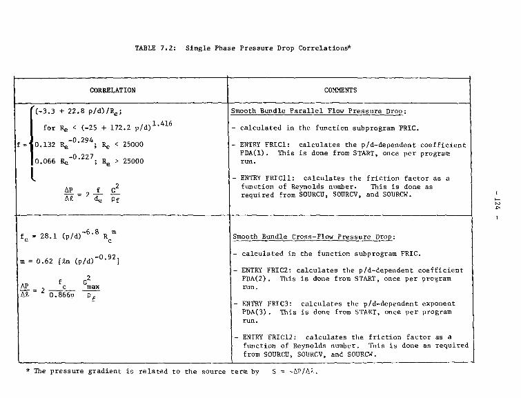
ITEMS 42 - 60 CORRELATIONS AND RESISTANCES
*2 loss factor for the centerline>etween the hot and cold side,MMV(I)
'araaeter -for selecting two-phaseMultipliers
Parameter for selecting voidfraction correlation
ee layout This array is used to indicate the location ofhe partition plate AKDIV(I) = 1.0 E+15, the-bend supports AKDIV(I) = k, or indicatehere no obstacles occur AKDIV(I) = 0. Theseoss factors are used to calculate the pressureoss relationship for the circumferential
velocity between the hot and cold sides <*se to>lates or supports; the tubes are handledndependently.
If ITPPD = 1-THOM used for parallel, cross andarea change
If ITPPD - 2-BAROCZY-CHISHOLM used for parallelcross and area change
If ITPPD = 3 - Separate correlations used
See Section 7.3
If IVF • 1, homogeneous correlationIf IVF = 2, Chisholm correlationIf IVF » 3, Smith correlation
AKDIV(I)
ITPPD
IVF
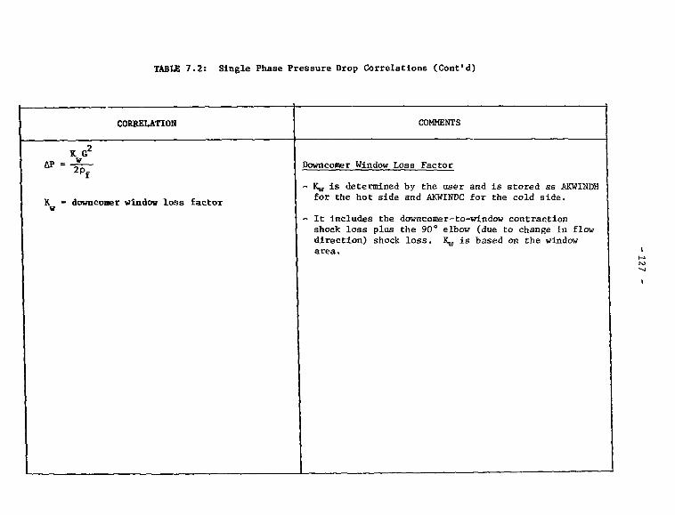
DATANo.AS
46
47
48
49
DESCRIPTION
k shock loss factor for the baffle)late resulting from area changecontraction and expansion)
k loss factor for the tube support>roached plate - based on shock
k loss factor for the largerbroached holes in a differentiallybroached plate
k loss factor for the smallerbroached holes in a differentiallybroached plate
plate
DATAVALUE
pproachre a
)evice Area
evice Lossactor
atne as datano. 45
Same as datano. 45
S&me as datano. 45
Same as datano. 45
REMARKS
ne loss for the baffle plate
(AKBL + f|) e£
This data is the AKBL portion which is theressure drop due to the contraction into thennulus between the drilled plate and the tubet is based on the approach area.
Also see data no. 58)
The tube support plates result in a pressuredrop due to an area change. This value isbased on the approach area.
In some designs, the first plate on the hotside has smaller broached holes near the shroucand larger broached holes near the center toencourage flow penetration. This factor isfor the area change in the central largerholes.
Shock loss for the outer small broached holes.See data no. 18 for the radial position wherethe hole size changes.
For some designs the tubes are not rolled intothe thermal plate and leakage through the plat
(AKTP + f ) ~~ a shock loss and a fric-
tion loss. This data ao. deals with the shock
loss. Again i t is based on the approach area
ARIABLENAME
AKBL
AKBR
AKBRL
AKBRS
AKTP
VALUE
DATANo.
<50
5 1
52
5 3
DESCRIPTION
Shock loss k factor for the shroudwindow on the cold side
Shock loss k factor for the shroudwindow on the hot side
Area ratio multiplier to determineReynold's number In gap in baffles.(See also data no. 58)
Area ratio Multiplier to determineReynold's number in gap in thermalplate
DATAVALUE
Lndov area *
mnular Area*an
0° Elbow^ s s » k90xpansionoss - kexl>
ame as datao. 50
Approacharea
" Aap
Gap area
• AgDiametricalclearance= c
See datano. 52
REMARKS
This pressure loss relationship i s based on a0° flow direction change and an expansionrom the downcomer annulus into the shroud
window. Both kgo° ant* kexp a r e based on Aan:
AKWINDC = <kgo. + k ) ( f ^ ) 2
an
Because the shroud window height may differ>etween the hot and cold s ide, a second lossfactor may he required.
The local Reynolds number i s :
D*v, *c 0*AKATB*V *c„ ._ loc appR ' u v
where: ARATB = (A Ik )*cap g
ARATTP - (A /A )*cap g
ARIABLENAME
AKWINDC
AKWINDH
ARATB
ARATTP
VALUE
DATANa
,54
DESCRIPTION
Loss factor calculated for thetwo-phase flow from the lastnodelied plane inside the shroudto the separator exit, k is
sepnormally given by the manufacturer
(based on V ) is calculatedsep
by user, and is generally much lessthan k
sep
DATAVALUE
ieparator.ess Factorksep
lontraction'actor = k
- total'P
flow arealefore enteing separatoi
= totalsepleparatorirea
REMARKS
To calculate the recircu-lation ratio the flow fromthe last modelled planeInside the shroud to thelast modelled plane out-side the shroud ismodelled one-dimension- id.'.*ly. CON1 is acombination of the lossfactors for the two-phasemixture. It is based onthe total flow as shownbelow- C0N2 (data no. 55)is the loss factor for thesaturated liquid flowingout of the separators.
From (1) to (2) - area contraction intoseparators.
APpviSEP
ASEP
where V « velocity inseparator
FLOW2
P ASEP ^EP 2p
From (2) to (3) - separator loss
AP - k,PV2.
SEP 2SEP FLOW2
2p
ASEP ASEP
VVAPP
TRIABLENAME
C0N1
VALUE
I
DATANo.
55
56
DESCRIPTION
Loss factor calculated for theseparated liquid flowing from thewater level to the last modelledplane in the downconer.
Parameter used to optimize theestimate of the recirculationratio.
DATAVALUE
-
REMARKS
'his loss is assumed to be a f r ic t iona l lossand treated as flow in a pipe.
. , -L pv2 L ^ 1 FLOW2 CON2*FLOW2
..flP f j - 2 - fD * 2 2 p - 2 p . •
2ADC
where CON2 = f i (-r^-)U *DC
L - XDOWN-X(L)-*see data no. 39D = Hydraulic Diam. = Diam. Clearance
A^ = Downcomer Area
p = Saturation Density of Water
0.316* R
R i s based on an estimate at thevelocity calculated from a recircu-lat ion r a t i o est imate.
DHPV RECIR * FLOWC FLOWe y P * A p*A^_
DC "c
This ra t io provides the code with an estimateof how the pressure drop through the modelledregion changes with recirculat ion ra t io( i . e . , to ta l flow). The code uses this valueto estimate the reci rcula t ion r a t i o needed tobalance the pressure loss against the drivinghead. C01M is set a t 2000. If severeconvergence problems are encountered, otherestimates ( i . e . , 2000 + 1000) should be t r i ed
VARIABLENAME
CON2
CON4
VALUE
3-
I
DATANo- DESCRIPTION DATA
VALUE REMARKS /ARIABLENAME VALUE
57 Thermal conductivity of the tubewall material
Obtain from material property data.CWALL
58 Friction pressure loss for thebaffle plate
BafflethicknessL
Diametricalclearance= D
Areaapproach
AAPP
Area gap* A.GAP
Also see data no. 45 and 52.
Ap •» [ARBL + ^ ] ~ -
The variable is concerned with the secondterm - the frictional loss.
f = .316/Re*25
L = thickness of baffle
D = diametrical clearance
Because this loss is based on approachvelocities, the area correction is included.
FLDB
Thus FLDB = .316 *L /AAPP\
\ GAP/
5 V- 25.. AP - [AKBL + FLDB * R ] *
DATANo.
59
60
DESCRIPTION '
Friction pressure loss for thethermal plate
Resistance due to fouling on theexternal surface of the tube
DATAVALUE
See data no.58
REMARKS
This variable stored the friction coefficientsmentioned in data no. 49 and 53.
PLOT _ £ * / W
2
/ . AP = [AKTP * FLDT * R£ ^ ] - ^
Fouling is assumed to act uniformly over thetube surface
VARIABLENAME
FLDT
RFOUL
VALUE
ITEMS 6 1 - 69 ARE OPERATING CONDITIONS
61
62
63
6A
Feedvater flow rate(kg/s)
Eeheater flow rate(kg/s>
Prinary flow rate (kg/s)
Saturation pressure of the primary(MPa)
flow rate.
Some designs include a reheater circuit.The flow returning from the reheater isassumed by the code to enter the steamgenerator at the top of the downcomer. Ifthere is no reheater circuit, set this valueto zero.
Flow rate for the whole unit
Used to calculate priin^ry properties
FLOWC
FLOWRH
FLOWTU
PPRI
DATANo- DESCRIPTION
DATAVALUE REMARKS VARIABLE
NAME VALUE
Saturation pressure of thesecondary (MPa)
Used to calculate secondary properties.Take trie value at the normal water level.
PS EC
Inlet quality of the primjrv fluid For a two-phase mixture, it is the actualqualitv. For a subcooled primary flow thisvalue is calculated using
n . _„ Enthaipv of Liquid-Saturation EnthaQLTu - *-•—• * - : : • • •
Latent Heat
OLTU
In i t i a l estimate of recirculationra t io (°C)
Tit a reci rculation rat io is not ad justed i orthe f i rs t 9 steps to allow the flowto se t t l e out. This* value serves ax ,inini t i a l condition.
Temperature of the feedwater (°C)
Temperature of the reheater returnflow
ITEMS 70 - 85 AKE UTILITY FEATURES AVAILABLE TO THK USER
The horizontal lines of data whichare to be included on the vert icalcut plots
In areas whore T pianes arc concentrated,onv may decide to IpaVi* out some I lines fromvertical plots so that tin* plotted arrows donot overlap. Normallv all the l ine ; would beplotted.
IF IIPLOT(I) = I - plot tht' lint-IF IIPf.OT(I) = 0 - skip the line
Note: rTP[,OT(r) must have- M entries
DATANo.
71
72
73
DESCRlPTluN
Selection of Che I position forwhich the hot side and cold side•ass flow will be calculated andprinted out
Selection of the K-planes to beplotted.
Selection of the I axial planes tobe plotted
DATAVALUE REMARKS
A subroutine MASSFLO has been set up to cal-ulate the mass flow in the axial direction
for selected planes. This information isrinted out any time the axial velocities ortensities are adjusted. Any number of I
planes may be specified up to NI.
This variable allows the user to select anynumber of Che circumferential planes forplotting. Note the K=2 and K~N planes areautomatically plotted to give the t i rs tframe and should not be requested again.
The plotting routine is set up to plot up toa maximum of 8 horizontal cuts. This variableis used to specify the I planes of interest.For example,
If IPLOTI = +10, the 10th plane will beplotted to the right of thevertical cuts - seeSection 6.3 for more details
If IPLOTI = -10, the 10th plane will beplotted on the left of thevertical plot. Note theremust be only 4 specified forthe left side (negativenumber) and 4 specified forthe right side (positivenumber) .
ARIABLENAME
IMASSF
IPLOTK
IPLOTI
VALUE
o
I
ATANo.74
75
76
77
DESCRIPTION
elect the variables to be printedut
Relaxation factors
Contour intervals for the plottingroutines
Last execution step
DATAVALUE REMARKS
This parameter allows the user to trim theutput down to variables cf specif ic i n t e r e s t .
If IPRINT = 1, the variable i s pr inted.If IPRINT = 0, the variable is skipped.
he order of variable s torage:TPRINT(l) = axial velocityIPRINT(2) = rad ia l veloci tyIPRINTO) = circumferential velocitvIPRINTM « mass fluxIPRINTO) = steam quali tyIPRLNT(fi) = primary temperatureIPRINTC7) = tube wall temperatureIPRINT(8) = s t a t i c pressureIPRINT(9) = density of mixtureIPRINT(IO) = local heat fluxIPRINTU1) = porositv
Allows the user to specifv the qual i tv con-tours of inlftt'st Can have up to 15 values.Zero valut" "r tlu- end of the arrav arei gnored.
Sots the last execution step. On completionof I.ASTEP iterations, the computation ceasesand detailed printing and plotting s tar ts .
VARIABLENAME
IPRINT
RELAX
TCON
LASTF.P
VALUE
JATANa
78
79
80
81
87.
83
DESCRIPTION
arameter to specify when, duringhe execution, plots are to be
made
arameter to specify when, duringthe execution, the variablespecified in IPRINT will be printed
out
Parameter for overriding the timelimit routine
Width of the plotting frame whenI-plaues are to be plotted both onthe left and on the right of the-vertical cut (see data no. 73)
Width of the plotting frame whenonly 1-planes are plotted on theright side of the verti"--" cut
Height of .... plotting frame
DATAVALUE
—
REMARKS
F PLOTO * 0, plots are never madeF PLOTO * 1, plots are made at the end of the
JobF PLOTO * 2 , plots are made after each
iteration
Note: If P1OTO - 2, a very long plot f i l ew i l l be produced. Careful se lect ionof values for IPLOTI and IPLOTK arenecessary, (data no. 72 and 73)
R1NTO i s set up the same as PLOTO in datao. 78. Note that PRINTO and PLOTO may be
reset in the logic to turn the PLOTTING andPRINTING routines on or off.
THIRST has been set up to print out a l l thevariables, make plots and write a RESTARTtape If the execution or INPUT/OUTPUT time hasbeen reached. To suppress this feature, setTIMELT to zero.
N• \ r\/r\1— XLl •"
TYI
11
— XL2 - ~ j
ARIABLEINAME
PL070
PRINTO
TIMELT
XLl
XL2
YL
VALUE
DATANo.
'84
85
DESCRIPTIONDATA
VALUE REMARKS
Sxcra integer Input locations- Data put intothese variables is common to al l subroutines
E>:tra real input locations.
VARIABLENAME
IEXTRA(I)1=1 ,9
REXTRA(I)1=1,9
VALUE
- 64 -
4.4 Preparation of the Input Data Cards
Once the data specification sheets have been completed, it is a
straightforward matter to transpose the requisite information
into data card form.
In THIRST, the data Is all processed through a routine called
READIN. READIN not only reads the data into core, but also
performs a detailed check on the completeness and precision of
the data supplied.
The course of execution of the program is directed by the
RESTART feature which is described in Section 5.2.
The input cards are assembled from the variable names and values
already detailed in the last two columns of the charts in
Section 4.3, immediately preceding.
The cards must adhere to the following rules :
(1) The first card must contain the title (1 to 40 columns) and
the RESTART value (word RESTART in columns 50 to 59 and
value in 60 to 69). If the RESTART name and value are not
included, READIN assumes a RESTART value of 1.
(2) All succeeding cards are read with the following format
s tatement
FORMAT (A9, 6 (A9, IX), A9)
- 65 -
The input cards for data arrays or single variables are,
ARP.YN
NAML
10
NN1
1
20
-1.
NAM2
30
6.2
-1
40
8750.5
ANAM3
50
1.0E+20
1.3456789
60
-.0068
ANAM3
70
-6.8E-4
180040.7
80
(NN Is the number of entries in the array called ARRYN. It is only
required for arrays 1MASSF, IPLOTI and IPLOTK.)
(3) The second card must contain the number of grid points NI, NJ,
NK, selected for each direction to provide READIN with the
counters for checking array data.
(4) From this point onwards, the data may appear in any order since
the variable name is always included with the data. READIN
treats each variable name and the corresponding data as a
variable set.
(5) It is possible that after a data deck is prepared, some tem-
porary changes are found necessary. In this case, a data
item may be changed in situ in the deck, or a single card
with the changed variable may be inserted immediately after
the NINJNK card. In such cases of multiple definition the
definition encountered earliest in the deck takes precedence,
so the new value will be used.
4.5 Sample Input Data Deck
The data deck sheets in Table 4.2 have been prepared from the
specification sheets of Section 4.3 according to rules outlined
in Section 4.4.
- 66 -
UJLL)
Ien
0 .
I
- 67 -
THIRST INPUT DATA SHEET
1 0
1 3 5 1 5 3l
l A K B l 1 6 0
A K T P 1 6 0
A R A T T P 0 . 0
C 0 N 4 2 0 0
E D F E E D 0 . 0
F 1 0 1 1 6 0
H I A 8 < 5 S
! r E E 0 L 8
I 7 P P 0 1
K C E N T C 7
0 G A P 0 . 0
P P R I 1 9 , 8
O L T U 0 . 0
R S H E U 1 . 4
T U B S H E T 0 . . 4 |
X V A N f 1 6 .
1 L 1 L 1 1 1
l l . 7 1 E +0 2 | l . 8 E • 0 2 I
0 I A K B R 1 . 5 A K B R L
0 B A K W I N D C 1 0 A K W I N D H
H e G A P 0 . 0 7 C 0 N 1
0 | C M A L I 1 6 . 7 D I A
6 5 • E D N O R M 1 . 2 2 E D S H R O X
0 I F I O W C 3 0 6 . 1 8 F L O W R H
0 I D O W N C 6 I D O W N H
I F E E D U 1 0 I P R H T
I U B E N D 3 0 I V F
K C E N T H 6 K F E E D L
3 P F W B U 3 1 2 5 P I T C H
7 9 P R 1 1 1 0 1 P S F C
4 4 R A D I U S 1 . 1 2 1 R E C I R
4 T I N C 1 7 6 . b 7 7 P I A T E
1 9 X D O W N 1 5 . 0 X L 1
0 V L T T 6 _[_ 1
1 • 1 • - •
_ - .
PAGE 3
II* It* Ik II1 1 1 "•Hi1 . " A K p P S fi n H J1 3 A R A T B 1 > 7 f» •; c . > B J
0 . 9 4 9 5 U N ! . 1 1 5 6 H
O . O 1 5 S 7 5 D I A [ If . 0 1 3 6 0 0 9 H
O . R F I D B ? 1 I ) I ) O H
2 3 . 7 F L O W T I J 2 4 8 4 . 9 3 H
7 F E E DB 13 B J2 0 I S H R D 3 1 B J1 J BR C H j 4 •9 I I A: T E P ! | b 0 H0 . 0 2 4 5 1 M" I 0 T n l l 1 •5 . 1 I P S H R D I ; i l l 0 . M
5 . 1 • - 1 - |0 . 6 1 5 I T R« I 1 ? 5 ' . 6 7 M
9 1 I x L :? 1 | h . 2 5 p j
1 I 1
~~ti—i=5 5""3;=|= ±::~! t | t |.T "17 .T. 1 , . —M
I
35
- 69 -
4. 6 The Standard Execution Deck
At this point, the major effort of preparing the data deck Is
complete. It is now necessary to enter the ThIRST job into the
computer system.
Execution control cards can vary between CDC computer
ins tallatior. s . However, the following decks are included as
examples, and operate satisfactorily on the CRNL system. For a
full explanation of CDC control cards, see references 13 and
14.
The decks consist of the following:
JOBCARD containing job name and account information
The above simple execution deck will execute the standard THIRST
code without reading or saving any RESTART data. Advanced
Execution Decks are discussed in Section 5.5.
4.7 Job Submission
A complete listing of the entire deck is given in Figure 4.5.
This may now be submitted to the CRNL system.
As turnaround time for a large job is not particularly fast, we
discuss in Chapter 5 some additional features of the code. Our
output will appear in Chapter 6.
- 71 -
THIRST ,B652 -EXAPPL,T50Ci I<J100 .ATTACH <CLDPl,TH I RSTPLt ID = THI:<ST)UP0ATEIC-DISC1FTN( I = O I S C , e = Tt-IRPCD>ATTACH(THIRST , ID=THI *ST)C O P Y L < T H I R S T , T H R I ' O L > , T M 5 S T 2 )ATTACH ( T A P E 6 0 . T h I R S T D A T A , I 0 = TATTACHIPLOTLIfl)LOSET(LIB=PLOTLie ,S lHST=PLOT-PLT>THIRST2(PL=300C0)I F E , R l . N E . O i J U r P .COHI1ENT. CATALCG RESTART TAPEC A T A L O G ( T A P E 6 0 , T H R S T 0 A T A , n = TE N O I F ( J U f P t7/8 /9•IDENT HYPOTH*O KOMON.l
READIN contains li&Ls of all the variables required by the code.
As the data cards are read, READIN searches through the list to
match input variable names vith the ones on its list. If the
subroutine can make the match, it stores the data in the
variable and removes the variable name from the list.
If READIN cannot match an input variable to one on Its list, it
issues the following message:
*** X CANNOT MATCH X VARNAME DATA ***
This message contains the input variable name and its value so
the user can trace the nature of the error. This error could
result from a misspelling of the variable name, from reading the
same variable twice, or- using Improper data. This error does
not result In a termination of the run. If a variable appears
twice, .READIN stores the first value and disregards the second.
If a variable is mispelled, READIN Ignores the variable and its
value, and thus the intended variable name will not be removed
from the list.
- 77 -
When the end of the Input deck (END OF FILE) is encountered,
READIN checks that all the variables on its list have been
initialized. Some variables may not be stroked off because they
are either mispelled or simply left out. If a variable name
remains, but has not been initialized, READIN issues one of the
following messages:
* THE FOLLOWING VARIABLE(S) HAVE NO INPUT DATA: VARNAME *
or * THE FOLLOWING ARRAY(S) HAVE NO INPUT DAT'.: VARNAME *
READIN then checks the value of RESTART and:
If (RESTART-+1) - READIN terminates the run
If (RESTART-+2or±1) - READIN uses the values stored on the tape
iade from a previous run and continues
executing, thus only variables to be
changed are required as input data.
5.3 Time Limit Feature
If the code senses that insufficient time remains to complete
another Iteration step and to print ana plot the output, it will
automatically call FPRINT for a printout, and call the WSTART
routine to write a RESTART tape. The user can subsequently
attach the RESTART tape and continue executing with additional
time.
Both execution time and input/output time are monitored, but
the time limit feature can be suppressed by setting the
- 78 -
parameter TIMELT to zero. If TIMELT is not set in input or is
set to 1 in the input deck, time remaining is checked at the end
of each iteration.
The statements: IFE(Rl.NE.0)JUMP
CATALOG (
ENDIF(JUMP)
should be included in the job control deck to catalog a RESTART
tape when a time limit is encountered.
5.4 Advanced Execution Deck
The simple execution deck introduced in Chapter 4 is sufficient
to run a standard '.HIRST job in which no RESTART tape Is read
or saved. For more advanced use, we now include an execution
deck which will permit the use of a RESTART tape, and also
permit certain code changes to be made, using the CDC program
library editor, UPDATE.
This "advanced use" deck contains three major segments:
(1) job control statements
(ii) update correction set
(iii) input data
Because the function of each section in the execution deck is
different, they will be explained separately. It is assumed
that the reader has! a basic understanding of the job card
sequence and the update routines available through the computing
system. A listing of the execution deck without explanations is
shown in Appendix C.
- 79 -
5.4.1 Job Control Statements
CardNo.
1
2
3
4
5
6
7
8
9
THIRST, B652-EXAMPLE,T500,I0100
ATTACH(OLDPL,THIRSTPL,ID=THIRST)
UPDATE(C=DISC)
FTN(I=DISC, B=THIRMOD)
ATTACH(THIRST, ID=THIRST)
COPYL(THIRST , THIRMOD, THIRST2)
ATTACH(PLOTLIB)
COMMENT.
LDSET(LIB-PLOTLIB,SUBST=PLOT-PLT)
Explanat ion
Attach the codestored on file nameTHIRST
Update the fileTHIRST with any codechanges in the associ-ated correction setand list on disc
Compile the fileTHIRST from DISC.SLore compiled file onTHIRMOD
Access standard THIRSTcode
Merge modificationsand standard code tocreate new programTHIRST 2
Attach library plot-ting package
- 80 -
CardNo.
10
11
12
ATTACH(TAPE60, THIRSTDATA,ID=THIRST)
THIRST2(PL=3OO0O)
IFE(R1.NE .0)JUMP.
Explanat ion
This card is requiredonly when the RE-START option is used(ABS(RESTART). GT.1)The data cataloguefrom a previousrun under file nameTHIRSTDATA with ID=THIRST and for CY=1will be attached andused to initialize thevariables. If RESTARTis 1, this card wi11have no useful purposeand should be omitted.
Execute the job andset the printing limitat 30000 print lines
If a RESTART tape hasbeen written eitherthrough a time limitor a negative value ofRESTART then Rl is setto one. If the pro-gram has not written adata RESTART tape thenRl = 0 and the execu-tion jumps to ENDIF(JUMP). Thus thiscard controls the se-quence to CATALOG onlywhen the data RESTARTtape exist s.
- 81 -
CardNo.
13
14
15
CATALOG(TAPE60, THIRSTDATA,ID=THIRST)
ENDIF(JUMP)
7/8/9
Explanat ion
Catalog the RESTARTtape
Point to which theIFE( ) card d i r e c t scon t ro l
End of record card
To enable the computer to allocate storage, the size of the grid
layout must be specified in the EXEC routine. The following
update correction may be used to change this allocation and is
included for example purposes.
CardNo.
16
17
18
*D EXEC.4
COMMON F(4320,13)
7/8/9
Explanation
Delete the fourth cardin EXEC
Reserve 13 arrays (11var iab les plus 2 work-ing spaces)• Eacharray contains NI*NJ*NK - 36*10*12 - 4320storage places
END OF RECORD
5.4.2 Input Deck
Unless the changes made above incorporate new input data, no
form changes in the deck of Chapter 4 are required.
- 82 -
6. THIRST OUTPUT
In this chapter, we present the basic output obtained from the
THIRST code. Possible variations of output are also discussed.
Output from THIRST is in both printed and graphical form.
The following paragraphs refer to sample output which appears
consecutively at the end of this section starting on page 99.
6.1 Printei Output Features
6.1.1 Preliminary Output
After the program logo, THIRST prints out the values in the
input deck. The arrays are printed first, the single integer
values second and the single real values last. All the error
messages related to the input are printed out in this section,
Figure 6.1.
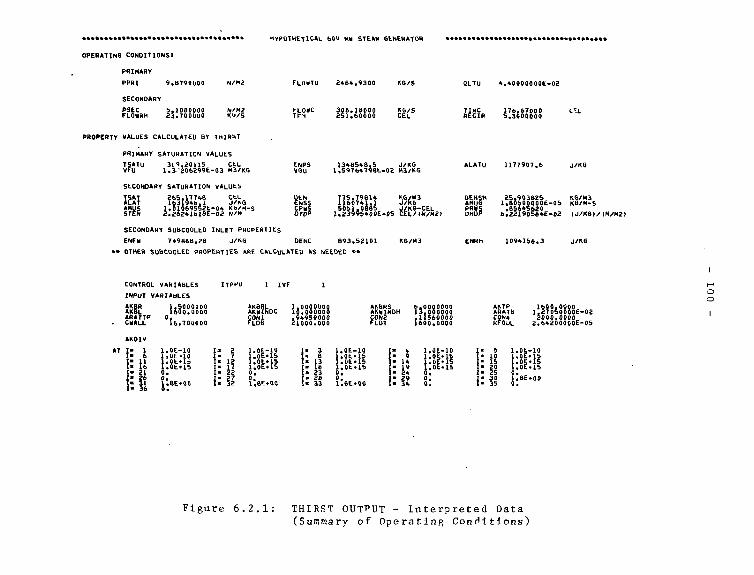
The next section of the printed output contains a summary of
all the input received by the code for this run and a summary
of the properties which THIRST has calculated from curve fits.
Figures 6.2.1 to 6.2.3 contain:
(a) Operating Conditions
- Primary
- Secondary
(b) Properties as Calculated by THIRST (using Curve Fits)
- Primary Saturation Values
- Secondary Saturation Values
- Secondary Subcooled Inlet Properties
(c) Output Selection and Control Parameters
(d) Geometrical Parameters
- 83 -
Figure 6.3 contains:
(a) The Grid Locations for Scalar and Vector Components
- The Axial Positions in Metres
- The Radial Positions in Metres
- The Circumferential Positions in Degrees
(b) Primary Fluid Flow Distribution per Typical Tube in kg/s
All the above output is generated in START before the
iteration procedure begins. The user has no control over
the format without altering the program logic.
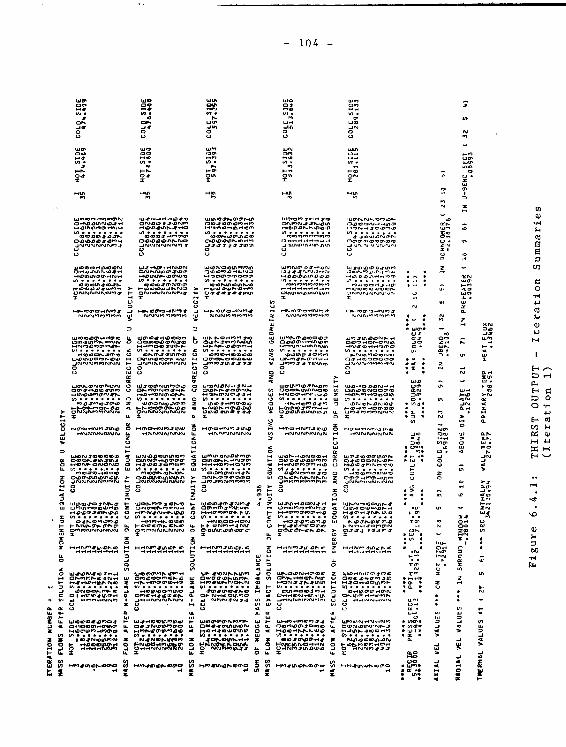
6.1.2 Individual Iteration Summary (Figures 6.4.1 to 6.4.5)
During the progression of the solution to convergence, the
following information is summarized on one page for each outer
iteration.
(a) Iteration: At the beginning of each iteration prior
to any further calculation, the EXEC routine prints the
outer iteration number.
(b) Hew Estimate of RECIR (only after the ninth step):
After the ninth iteration, the program begins to calculate
the RECIRculation ratio. Because the solution technique
is iterative, the value will change until the solution
approaches convergence.
(c) Mass Flows at Planes of Interest: The mass flows are
calculated at I-planes selected by the user. The user
can chooBe any or all of the I-planes by using the IMASSF
- 84 -
parameter (see data no. 71, Table 4.1). The mass flow
Information is preceded by a line indicating the point
within the iteration step at which these calculations were
performed. The mass flows at designated I-planes are
plotted in five columns of eight entries each for a maximum
of forty positions, if required. The mass flows are given
for both the hot and cold side. The calculations are made
in MASSFLO. MASSFLO is called whenever the axial velocity
or local density is changed.
(d) Summary of Overall Performance Variables and the
Convergence Indicators: At the end of an iteration step, a
summary of the overall performance variables and the
convergence indicators are printed. The user has no direct
control over this format. The information provided
Includes:
RECIR Recirculation ratio used for this iteration
PRESS DROP
in Pa
PRIM H.T.
in MW
is the pressure drop between the average
pressure at the last I-plane (1,-plane)
inside the shroud and the average
pressure at the last I plane (L-plane)
outside the shroud in the downcomer .
Is the net amount of heat given up by the
primary fluid
- 85 -
SEC H.T. is the amount of heat picked up by the
in MW secondary. This includes the heat required to
raise the feedwater and reheater drain flows
to saturation, plus the heat absorbed in
evaporating the secondary liquid.
NOTE PRIM H.T. should equal SEC H.T. when convergence
has been achieved.
AVG/OUTLET/QUAL average outlet quality
SUMSOURCE is the summation of the absolute value of the
mass imbalance for each control volume
normalized by dividing by the total flow. This
indicator should approach•?ero with conver-
gence ,
MAXSOURCE (2,7,11) is the largest mass imbalance
normalized by dividing by the total
flow in the modelled region. The
location is gi"en in the brackets as
1-2, J-7, K-ll. If the location
remains fixed, and the imbalance is
significant, the use should examine
the region for a possible error in
that area•
(e) Summary of Local Values; The last section of the iteration
by iteration printout summarizes local values at strategic
locations in the model. The locations are fixed in the
code at such points as window inlets, above the preheater,
in the downcomer, etc.
- 86 -
Three sets of variables - AXIAL VELOCITY, CROSS FLOW
VELOCITIES and THERMAL VALUE are printed. The location of
each variable is described including its (I,J,K) coordi-
nates. If the user wishes to change the locations to be
printed, the OUTPUT subroutine must be altered.
The overall values (d) and local values (e) are printed out
in OUTPUT. OUTPUT can be called at any point in the.
execution if the user desires to. At present it is called
at the end of each iteration step.
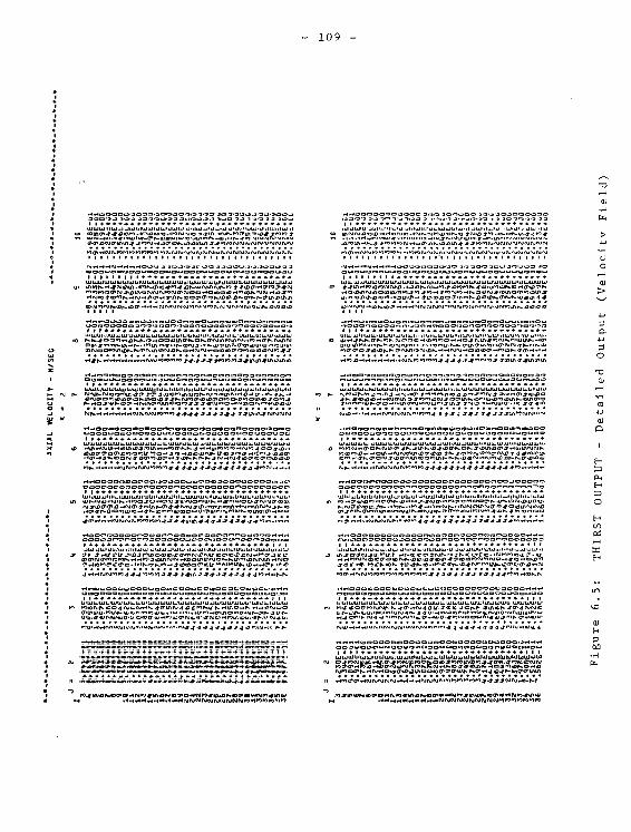
6.1,3 Detailed Array Printout (Figure 6.5)
The last type of printed output, again under user control, is
the complete printout of selected variables at every active node
in the model. The format for the printout is
XXXXXXXXXX VARIABLE NAME (1) XXXXXXXXXX
K=2
1 = 2 J = 2 J = 3 J=4 J=M
1 = 3
1 = 4
II=L
- 87 -
1 = 2
1 = 3
1=4
J=3 J=4
K=3
-J=M
K=N
J = 2 J=3 J=4 -J=M
1 = 3
1=4
II-L
XXXXXXXXXX VARIABLE NAME (2) XXXXXXXXXX
etc •
This printout can be very long depending on how many variables
are specified for printout. Figure 6.5 shows the first page of
a detailed array printout of axial velocity obtained by setting
IPRINT(I) to 1. Each selected variable takes a similar format
and each generates five pages of output for K»12, so the feature
should be used with caution. Variables to be printed may be
selected by the input variable IPRINT.
If IPRINT(NV) is entered non zero, the array of values for
variable NV is printed, where NV is selected as follows:
- 88 -
NV
NV
NV
NV
NV
NV
NV
NV
NV
NV
NV
= 1 -
= 2 -
= 3 -
= 4 -
= 5 -
= 6 -
= 7 -
— Q —
= 9 -
= 10 -
= 1 1 -
axial velocity
radial velocity
circumferential velocity
mass flux
steam qual1ty
primary temperature
tube wall temperature
s t a t i c pressure
density
heat flux
porosity
This printout is generated by the FPRINT subroutine. The PRINTO
parameter calls FPRINT as follows:
If PRINTO = 0 - the FPRINT array is never called
- this would be used where the user is interested
in the plots only
If PRINTO = 1 - che FPRINT array is called after exit from the
iteration loop at the end of the run
If PRINTO = N - the FPRINT array is called every (N-l) iteration
steps. This tends to create large output files
and thus is only used for debugging p rposes.
Careful selection of the IPRINT (NV) parameter
is suggested.
- 89 -
6.2 Graphical Output Features
The plot routines have been set up to produce:
(a) quality contours
(b) velocity vectors
(c) mass flux vectors
for any planes of interest.
Quality contour values are specified by TCON in the input deck.
Up to 15 contour intervals are allowed. If less than 15
contours are desired, then set the remaining position of the
TCON array to zero and the plotting subroutine ignores them.
Velocity vectors are determined by first interpolating each
velocity component to the grid nodes. The two velocity
component? lyli.% in the plane of interest are added vectorlally.
The resultant vector is printed as an arrow with its length
indicating magnitude ?nd angle indicating direction. Mass flux
contours are determined by multiplying the velocity vector
calculated earlier by the local density.
Two plotting formats are available to the user:
(a) Full Diameter/Horizontal Cut Composite
(b) Vertical Cut Composite
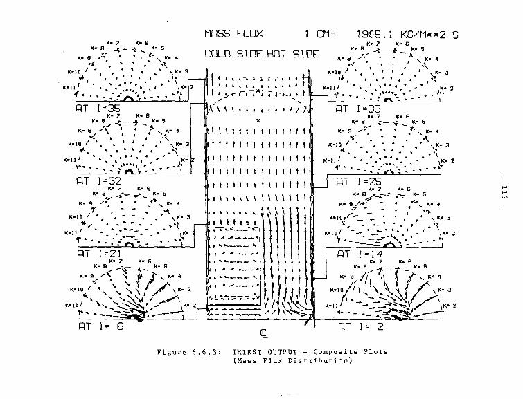
Full Diameter/Horizontal Cut Composite
This composite includes plots of values of the K-2 and K-N
planes which lie next to the line of symmetry. These are put
out by the plot routine automatically. Included on this frame
- 90 -
a r e u p t o e i g h t h o r i z o n t a l c u t s t h r o u g h t h e m o d e l l e d r e g i o n
corresponding to eight axial lines specified by the IPI.OTI
p a r a m e t e r . T h e s e l e c t i o n o f h o r i z o n t a l c u t s is n a d e b y t h e u s e r
i n t h e i n p u t d e c k , b y s p e c i f y i n g t h e n u m b e r of d e s i r e d I - p l a n c s
( m a x i m u m o f e i g h t ) . A n e g a t i v e s i g n in f r o n t o f t h p s p e c i f i e d
I - p l a n e p o s i t i o n s C h e p l o t o n t h e l e f t o f t h e F u l l D i a m e t e r
P l o t , o t h e r w i s e t h e p l o t a p p e a r s o n t h e r i g h t o f t h e F u l l
D i a m e t e r P l o t . N o m o r e t h a n f o u r I - p l o t s f o r t h e l e f t a n d f o u r
f o r t h e r i g h t m a y b e s p e c i f i e d . I f o n l y f o u r i - p l a m s a r e
s p e c i f i e d , a l l t h e p l o t s s h o u l d a p p e a r o n t h e r i g h t a s c h e
p l o t t i n g r o u t i n e w i l l r e d u c e t h e f r a m e s i z e . F. >: a m p i e s o f t l i i s
composite are given in Figure 6.6, which depicts quality,
velocity and mass flux profiles consecutively.
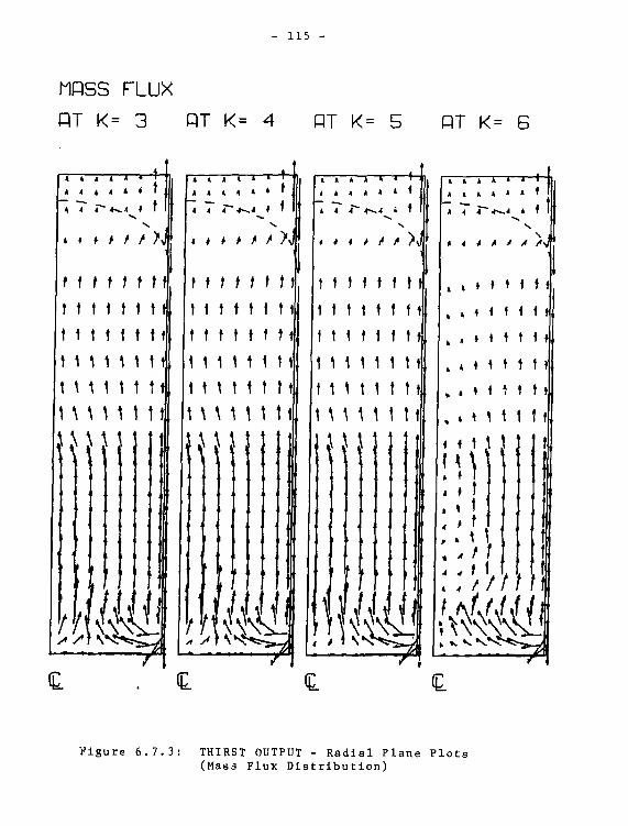
Vertical Cut Composite
The second plot format is a composite of four vertical cuts
corresponding to circumferential planes. The number and indices
o f K - p l a n e s to b e p l o t t e d a r e s p e c i f i e d b y t h e p a r a m e t e r T P 1 . D T K .
There is no limit on the number of K-planes to be selected.
Examples of this composite for quality, velocity and mass flux
profiles are given in Figure 6.7.
In some grid layouts, axial planes are grouped together to
provide greater detail. Unfortunately, when velocity or mass
flux vectors are plotted, they tend to overlap. To ensure
clarity of the plots, an additional plot parameter called 11 PLOT
has been introduced. If IIPLOT (I) = 1, the values on that
I-plane are Included on the vertical cut plots. If IIPLOT (I) =
0, the corresponding I-plane values are left off the plot.
- 91 -
The user has control over the plotting frame size. For the
first composite, the width is specified by "XL1" and "XL2". If
horizontal plots are made on the left and on the right of the
vertical cut, the routine usss the wider plotting frame
specified In XL1. If other horizontal plots appear only on the
right, the routine uses the narrow plot XL2. The height for all
plots is YL. The length to width ratios of the plots may not be
in proportion to the actual design, as the width may be
increased to add clarity. Scaling factors are determined by the
code .
The plotting routines can be called at any point in the code by
the statement CALL CONTOUR. The parameter PLOTO has been
introduced to control the calling of the plot routines.
If FLOTO = 0 - the plot routine is never called. This may ^e
used where the user wants only a printout.
If PLOTO * 1 - the plot routine Is called at the end of the
program.
If PLOTO « 2 - the plot routine is called at the end of each
iteration. This leads to a very long plot life.
PLOTO is set in the input deck. PLOTO and PRINTO can be reset
In the program to initiate the plotting and printing function.
- 92 -
6.3 Interpretation of the Output
Having discussed the layout of printed output we now turn again
to the printed output, Figures 6.1 to 6.5, to examine its content
and its significance.
The first page of printout, Figure 6.1, contains a summary of
all the data introduced through the Input deck. No error
messages of consequence were issued and a comparison with the
data sheets indicfcf.es that the data has been introduced
correctly•
The second, third and fourth pages (Figure 6.2) contain input
values and calculations made with the input. The operating
conditions should be checked against the information sheets.
Property values generated by the code should be checked against
values in standard tables. Correlation data should be verified.
The input/output parameters are simply informative. Finally,
the geometric data should be verified against drawings or data
sheets. The modelled heat transfer area should be examined to
ensure that it is not radically different than the prescribed
value. Although the correction factor will correct the modelled
tube surface, a large discrepancy may indicate an error in
treating the tube-free lanes or in the location at the start of
the U-bend (IUBEND).
The main grid location (Figure 6.2) and particularly the
displaced grid locations should be checked to ensure proper
modelling of flow obstacles. For instance, the displaced grid
- 93 -
at 1=13 for the axial velocity should in this case correspond to
the elevation of the first inner baffle. The primary fluid
flow, also Included on this page, is distributed to reflect the
different tube lengths. Scanning the distribution, one should
see a drop in primary flow along the K=2 plane with increasing
J.
When satisfied with the validity of the Input, one can proceed
to examine the iteration by iteration output (Figure 6.4). Of
prime importance is the line bounded by asterisks. Part of
this line contains the overall parameters which must converge on
single values - RECIR, PRESS DROP, PRIM and SEC HEAT TRANSFER
and QUAL. The last two terms are the sum of the absolute value of
the mass imbalance over all control volumes and the maximum mass
imbalance at an indicated control volume. These should
approach zero at convergence. By examining the line of
printout as the solution proceeds, one can assess whether the
solution is converging to a single solution or oscillating
slowly about the solution.
Assuming that the run has completed normally without any
execution errors, we will concentrate on the last several
iterations to verify that a converged solution has been
obtained. Later in this section we will discuss handling runs
that terminate in execution errors.
Comparing Iterations 58, 59 and 60, Figures 6.4.3, 4 and 5, we
observe that RECIR has converged to the fourth significant figure,
which Indicates that the pressure distribution has also
converged.
- 94 -
Examining the mass flows at various stages In the iteration
step, we see that the values are basically stable. Minor
changes can be expected due to the nature of the finite
difference technique; however, a swinging from or.? value to
another would indicate an inconsistency in the modelling between
stages. If the swinging is significant, further debugging of
the logic should take place.
In the middle of the mass flow printout is the SUM OF RING
(WEDGE) MASS IMBALANCE. As explained in earlier sections,
continuity is enforced simultaneously over groups of control
volumes. Control volumes are grouped alternatively into wedge
and ring geometries. The MASS IMBALANCE should approach zero at
convergence; however, the level indicated is considered
acceptable.
At the end of the run we also should be satisfied that the
pressure drop value is stable, that the heat transferred out of
the primary (PRIM H.T.) is equal to that absorbed by the
secondary (SEC H.T.) and that the source terms are sufficiently
small. The location of the maximum imbalance is given in
brackets after the MAX SOURCE. This information can be useful
during debugging to indicate trouble areas. If the location
remains fixed and the imbalance fairly high, one should examine
the region for a modelling error.
Tht last three lines on Figure 6.4.5 contain local values of
thermal and hydraulic variables. These values should be
compared with earlier iterations to ensure that they have
converged. The positions shown in brackets have been selected
to monitor variables because they are particularly sensitive
areas.
- 95 -
When we are content that the solution has converged, we should
examine the printouts to check numbers against Intuition and
then examine the plots to verify -hat flow and quality patterns
are consistent. These outputs will not provide additional
evidence of convergence but will enable the user to intuitively
verify the results. For instance, the quality profiles on the
1=2 plane could be superimposed over the velocity vectors to
verify that the velocities are concentrating near the point of
highest quality. The velocity vectors in the D-bend should
indicate an outwards radial flow to the lower resistance
regions. The flow around the baffles should be well defined-
Having examined the output, we conclude that, for this example,
the solution has converged.
6.4 Treatment of Diverging Solutions
If the solution has not converged, we should either restart the
program and continue for mjre iteration or examine the modelling
for errors. It may be necessary to use lower relaxation factor
to promote convergence.
If the solution terminates on an execution error or will not
converge, the user will be required to debug the model. The
efficiency of the user's debugging methods will improve only
with experience. To assist in debugging, the following
potpourri of examples is included:
(a) If the program has terminated before completing one
Iteration, it Is likely that insufficient input data has
been given or that the array sizing doesn't match the
arrays referenced. One can identify the line In which the
error occurred and generally find the error using an
"OPT-O" on the FTN card.
- 96 -
(b) If the program fails after the eighth iteration, examine
the RECIR subroutine because it is called after the eighth
1teration.
(c) If the program terminates with an error message "ARGUMENT
LESS THAN ZERO", this is most likely generated by quality
values greater than 1 arising from a very high pressure
gradient (the user should refer to DENS to see how pressure
affects quality). The high pressure gradient generally
occurs when a gross Inconsistency in the treatment of flow
obstacles occurs between various stages of the iteration
procedure. Large pressure corrections are required to
maintain continuity. The stage within the iteration that
contains the Inconsistency can be determined by examining
the mass flows printout.
(d) Large swings in thermal values generally indicate a problem
in the heat transfer subroutine source terms, especially
if a new correlation has been introduced. Reduce the
relaxation factor for T w to promote stability.
(e) If the solution is not converging and the reason is not
clear, it may prove useful to call for plots for several
succeeding iterations. The plots should then be super-
imposed to identify regions that are oscillating. In this
way, the region(s) of possible modelling errors can be
pinpointed- One could also call for FPRINT output for
several succeeding iteration?.
- 97 -
>
(f) If the FPRINT array is called and columns of zeros appear
in the output or If a mode error occurs, check that the
common card in EXEC hich sets the size of the F-array has
been dimensioned correctly.
(g) If the PRIM H.T. is different than the SEC H.T., the
problem is most likely located in the SOKRCH routine where
the heat transfer source terms are calculated. Check that
the no-tube regions are bandied correctly and that any new
correlations are used correctly.
(h) If the results seem to oscillate between two sets of
values, check the wedge and ring routines to ensure con-
sistency of treatment. These routines are used on alter-
nate steps.
(I) If the flow oscillates between the hot and cold si.ie shroud
windows, examine the treatment of flow obstacles in the
downcomer.
(j) If resistances appear to be incorrect, one can print out
the DU, DV and DW arrays after the CALCW subroutine. These
arrays can be printed using the logic in FPRINT. They
contain all the resistances in the model and can be checked
to see if any resistances are out of line.
(k) The pressure correction generated in RINGS1 and WEDGES1 can
be printed out to Identify trouble spots. Printing out the
pressure corrections for the CALCPK and CALCPIJ is more
involved since the control volumes are not grouped.
- 98 -
(1) When RESTART Is set to -1, there should be no control card
that attaches a RESTART tape to the program. An ATTACH
statement is necessary when RESTART is set to +2 and +3.
If an ATTACH statement Is present when RESTART equals -1,
the program will run and output will be printed, including
any plots, but the RESTART tape requested by negative value
of RESTART will not be made and you will get a DMPX. The
dayfile will indicate "ILLEGAL I/O REQUEST", the "FILENAME
..." and "FET ADDRESS..." as well as "WRITE NOT AT EOI ON
PERMANENT FILE".
(m) Finally, the user should document convergence problems and
their solution so that future problems will be easier to
A X I A L VEL VALUES • * • CrJ HOT S I D E ( 2 3 5 5> Oh C O L O S I D E i 2 3 5 9 ) I N U6END I 32 5 51 I N OCWNCOMER ( 23 10 5 )4 . J . 4 7 2 3 . 9 8 7 3 3 2 . 7 4 9 7 9 - 2 . 3 6 4 0 B
R A O I A L IE!L VALUES • • • I K SHROUD rflNDOK < 6 1 0 5 1 ABOVE O I V P L A T E ( 2 1 5 7 ) I N P S E K E i T E R ( I f 5 61 I I I U -SENO SECT- . 6 3 3 7 3 . 8 1 7 9 5 . E S 2 3 E . 6 6 5 0 2
This chapter details the content and sources of (i) the
thermodynamic property data for light and heavy water, and
(ii) the empirical correlations used in the THIRST code.
Normally the user will not change these. However, if it is
desired to investigate the possible effect of introducing
different correlations, this may be accomplished by simple
coding changes to the routines mentioned below.
The user can easily insert his own property functions to cover
different temperature and pres: ure ranges or different fluids.
Pertinent information related to each property or parameter
calculated in PROPRTY is listed in Table 7.1.
7 .1 Thermodynamic Properties
Heavy water and light water saturation and subcooled properties*
as well as property-related parameters are calculated in the
function subprogram PROPRTY. Saturation properties are computed
from polynomial functions of user-specified saturation
pressures** whereas subcooled properties are calculated from
polynomial functions of temperature and/or enthalpy.
The user can easily insert his own property functions to cover
different temperature and pressure ranges or different fluids.
Pertinent information related to each property or parameter
calculated in PROPRTY is listed in Table 7.1.
Heavy water primary properties are based on an AECLproprietary program. Light water secondary properties arebased on the ASME steam tables.
THIRST is set up to handle a two-phase primary fluid. Forsteam generators which have a subcooled primary fluidentering the tube bundle, the primary inlet pressure isspecified rather than a saturation pressure. The subcoolingis specified by defining a negative thermodynamic quality.
TABLE 7.1: Fluid Properties and Parameters
PROPERTY OR PARAMETER
Secondary Fluid Saturation Properties:
Pressure (MPa)
3Liquid Density (kg/m )
Steam Density (kg/m )
Saturation Temperature (°C)
Enthalpy of Vaporization (j/kg)
Liquid Saturation Enthalpy (J/kg)
Liquid Viscosity (kg-m -s )
Liquid Specific Heat (j-kg -°C )
Liquid Prandtl Number
Steam Viscosity (kg*m~ -s~ )
Surface Tension (N/m)
Change in Saturation Temperature perUnit Change'in Pressure (°C/Pa)
FORTRANNAME INPROPRTY
PSEC
DEN
DENSM
TSAT
ALAT
ENSS
AMUS
CPWS
PRWS
AMUG
STEN
DTDP
ACCURACY OFPOLYNOMIALEXPRESSION
(Z)
specified byuser
0.00
0.01
0.03
0.01
0.01
0.05
0.00
0.02
0.00
0.02
COMMENTS
- Secondary Fluid Saturation Proper-ties are expressed as polynomialfunctions of the user-specifiedsecondary saturation pressure PSEC.Each function is valid over thepressure range of 4 MPa to 6 MPa.The properties are calculated inthe function subprogram PROPRTY,ENTRY PR0P1.
- DTDP is the derivative of the TSATversus PSEC expression.
- DHDP is the derivative of the ENSSversus PSEC expression.
TABLE 7.1: Fluid Properties and Parameters (Cont'd)
PROPERTY OR PARAMETER
Change in Saturation Liquid Enthalpyper Unit Change in Pressure
Chen Correlation Parameters:
Primary Fluid Saturation Properties(Heavy Water):
Pressure (MPa)
Saturation Temperature (CC)
Liquid Saturation Enthalpy (J/kg)
Enthalpy of Vaporization (J/kg)
Liquid Specific Volume (m3/kg)
3Steam Specific Volume (m /kg)
FORTRANNAME INPROPRTY
DHDP
AKBOXTTK
PPRI
TSATU
ENPS
ALATU
VFU
VGV
ACCURACY OFPOLYNOMIALEXPRESSION
(%)
user-specified
0.01
0.02
0.03
0.07
0.47
COMMENTS
- The Chen correlation parameters aredefined in Section 7.3. The twoparameters are expressed as functionsof various saturation properties.
- Primary Fluid Saturation Propertiesare expressed as polynomialfunctions of the user-specifiedprimary saturation pressure, PPRI.Each function is valid for heavywater over the pressure range of7 MPa to 11 MPa. The properties arecalculated in PROPRTY, ENTRY PR0P1.
TABLE 7.1: Fluid Properties and Parameters (Cont'd)
PROPERTY OR PARAMETER
Feedwater Subcooled Properties:
Feedwater Temperature (°C)
Reheater Drains Temperature (°C)
Feedwater Enthalpy (J/kg)
Reheater Drains Enthalpy (J/kg)
3Feedwater Density (kg/m )
FORTRANNAME INPROPRTY
TINC
TRH
ENFW
ENRH
DENC
ACCURACY OFPOLYNOMIALEXPRESSION
ser-specified
ser-specified
0.1 at 5 MPa0.2 at 4 to6 MPa
0.1 at 5 MPa0.2 at 4 to6 MPa
0.1 at 5 MPa0.2 at 4 to6 MPa
COMMENTS
- The subcooled feedwater propertiesare calculated from the user-specified temperatures TINC andTRH. The properties are calcula-ted in PROPRTY, ENTRY PR0P1 andare valid for the temperature rangeof 150°C to saturation.
TABLE 7.1: Fluid Properties and Parameters (Cont'd)
PROPERTY OR PARAMETER
Primary Subcooled Properties(Heavy Water):
Temperature (°C)
Heat Transfer Coefficient Parameter,RCONVA
r i -l °-67 i i -° - 4 7
(W-m -L-°C L) (kg-m -s l)
-1 1 °-33l(j-kg --c A) I
Secondary Subcooled Properties(Light Water) :
Liquid Viscosity (kg-nf 1-s~1)
FORTRANNAME INPROPRTY
ROP (ENTRYPROP 2)
PROP (ENTRYPROP3)
PROP (ENTRYPROP4)
ACCURACY OFPOLYNOMIALEXPRESSION
(%)
0.01 at 9 MPa0.30 at 7 to11 MPa
0.12 at 9 HPa0.50 at 7 to
11 MPa
0.96 at 5 MPa2.5 at 4 to6 MPa
COMMENTS
- The primary temperature and the heattransfer coefficient parameter arecalculated from polynomial functionsof enthalpy. They are valid overthe temperature range of 245°C tosaturation.
- The heat transfer coefficientparameter (RCONVA) is defined inSection 7.3.
- All subcooled properties (ENTRYPROP4 to PR0P8 inclusive) are cal-culated as polynomial functions ofenthalpy and are valid over thetemperature range of 150°C to satura-tion.
oI
TABLE 7.1: Fluid Properties and Parameters (Cont'd)
PROPERTY OR PARAMETER
Temperature (°C)
Liquid Specific Heat (J*kg~ *°c" )
Liquid Prandtl Number
Liquid Density (kg/m )
Derivative of Saturation Pressurewith Respect to Temperature forChen Correlation (Pa-'C"1),(Section 7.3).
FORTRANNAME INPROPRTY
ROP (ENTRYPROP 5)
>ROP (ENTRYPROP6)
PROP (ENTRYPROP7)
PROP (ENTRYPROP8)
?ROP (ENTRYPROP9)
ACCURACY OFPOLYNOMIALEXPRESSION
0.1 at 5 MPa0.1 at 4 to6 MPa
0.3 at 5 MPa0.6 at 4 to6 MPa
0.5 at 5 MPa1.1 at 4 to6 MPa
0.1 at 5 MPa0.2 at 4 to
6 MPa
COMMENTS
- 122 -
7.2 Range of Application
The thermal-hydraulic data in the THIRST code is limited to the
following range of operating conditions:
Primary - heavy water; 7 MPa to 11 MPa inlet pressure;
subcooled to two-phase inlet (the overall temperature drop
should be such that the outlet temperature is not less than
245°C
Secondary - light water; 4 MPa to 6 MPa mean pressure;
feedwater temperature range of 150°C to saturation
If it becomes necessary to investigate different fluids or
conditions outside of the above ranges, the user must redefine
the appropriate property polynomial functions in the PROPRTY
subprogram*
7.3 Empirical Correlations for Flow and Heat Transfer
All the fluid flow and heat transfer correlations used in THIRST
are given In Tables 7.2 to 7.6.
The secondary side smooth bundle friction factors and heat
transfer coefficients are calculated in the function subprograms
FRIC and HTF, respectively. These relationships are valid for
equilateral triangle tube bundle arrays with pitch-to-diameter
ratios ranging from 1.3 to 1.7. The user can easily insert his
own correlations if those coded are unsuitable for his
application.
Tube support plates and baffle plates are assumed to resist the
flow only in the axial direction. The tube support plate
pressure loss is assumed to result entirely from the sudden area
- 123 -
change through the plate; friction resistance is ignored. The
baffle plate pressure loss Is a combination of shock loss plus
frictional loss in the reduced area. The value of the loss
factors are determined by the user. The method for calculating
these factors is shown in the data sheets.
Two-phase pressure drop correlations, in the form of
multipliers, are coded in the subroutine TWOPH. The user can
choose various combinations of these multipliers by setting the
appropriate value for the index ITPPD.
The mixture density distribution is calculated in the subroutine
DENS. The user has the option of calculating density using the
homogeneous, the Smith*, or the Chlsholm* void fraction
relationships by setting the appropriate value of the index
IVF.
The Chen* correlation is the only two-phase heat transfer
relationship used in THIRST. Because of their non-linear
nature, boiling heat transfer correlations require considerable
coding work to ensure convergence and stability. In view of
this, it is recommended that the user consult with the authors
if he wishes to insert another boiling heat transfer
relationship •
These correlations are discussed in detail in reference 5.
TABLE 7.2: Single Phase Pressure Drop Correlations*
CORRELATION
f = '
(-3.3 + 22.8 p /d) /R e ;
for Rg < (-25 + 172.2 p / d ) 1 ' 4 1 6
0.132 Re " " ^ ; Rp < 25000
0.066 Re" 0 " 2 2 7 ; Re > 25000
AP f G2
AX. Z de p f
f c = 2 8 . 1 ( p / d ) ~ 6 - 8 Rcm
m = 0.62 [Jin ( p / d ) " 0 * 9 2 ]
2AP „ f c GmaxAJ, ' 0 .866p p f
COMMENTS
Smooth Bundle Pa ra l l e l Flow Pressure Drop:
- calculated in the function subprogram FRIC.
- ENTRY FRIC1: calculates the p/d-dependent coefficientPDA(l). This i s done from START, once per programrun.
- ENTRY FRIC11: calculates the f r ic t ion factor as afunction of Reynolds number. This i s done asrequired from SOURCU, SOURCV, and SOURCW.
Smooth Bundle Cross-Flow Pressure Drop:
- calculated in the function subprogram FRIC.
- ENTRY FRIC2: calculates the p/d-dependent coefficientPDA(2). This i s done from START, once per programrun.
- ENTRY FRIC3: calculates the p/d-dependent exponentPDA(3). This i s done from START, once per programrun.
- ENTRY FRIC12: calculates the f r ic t ion factor as afunction of Reynolds number. This i s done as requiredfrom SOURCU, SOURCV, and SOURCW.
* The pressure gradient is related to the source term by S = -AP/AP-.
TABLE 7.2: Single Phase Pressure Drop Correlations (Cont'd)
CORRELATION
r =
64/Re; Rg < 2000
0.316 R " ° ' 2 5; R > 2000
e e —
AP / f G2
A* \2dJ pf
K t 02
K = tube support loss factor based onapproach area
COMMENTS
Downconier Annulus Pressure Drop:
- calculated in the function subprogram FRIC.
- ENTRY FRIC13: calculates the friction factor as afunction of Reynolds number. This is done asrequired from S0URCU, and S0URCW,
Tube Support or Broach Plate Pressure Drop:
- the loss factor is stored as AKBR in code.
- Kt based on the contraction into the support plateand the expansion out of the plate, dt is based onthe approach area before the contraction.
TABLE 7.2: Single Phase Pressure Drop Correlations (Cont'd)
AP =
hA2Alt
c
fl
Gl
CORRELATION
G2
2 P f
= baffle loss factor based on approacharea
= approach area
= local area
= baffle thickness
= diametral clearance
= 0.316 (- -)
= local mass flux
local frictionfactor
COMMENTS
Baffle Pressure Drop
- Kj, is the shock loss factor basedinto the baffle and expansion outis based on the approach area.
on a contractionof the baffle. It
- fl is the friction factor which varies with Reynoldsnumber. The constant portion is stored in FLD (seedata sheets for discussion of FLD calculation).
TABLE 7.2: Single Phase Pressure Drop Correlations (Cont'd)
CORRELATION
K G 2
K = downcoraer window loss factorw
COMMENTS
Downcomer Window Loss Factor
- Kf, is determined by the user and is stored as AKWINDHfor the hot side and AKWINDC for the cold side.
- It includes the downcomer-to-window contractionshock loss plus the 90° elbow (due to change in flowdirection) shock loss. K^ is based on the windowarea.
TABLE 7 . 3 : S e p a r a t o r P r e s s u r e Loss
CORRELATION
c/
C = K /A2
1 s s
Ks = separator loss factor
A = total separator throat area
W = total mass flow through separators
p = homogeneous mixture density
COMMENTS
C. = C0N1. CON1 is calculated by the user and readin as input. The separator loss factor Ks and thetotal separator area As should be available as designspecifications for the steam generator of interest.
1
to
TABLE 7 . 4 : Two-Phase P r e s s u r e Drop C o r r e l a t i o n s
CORRELATION
/AP\ .2 /AP\
[ w - * [~Ki)0V / t p \ fio
homogeneous:
Thom:
COMMENTS
- All two-phase pressure drop mul t ip l ie rs are calculatedin the subroutine TWOPH, and cal led from the SOURCU,SOURCV and SOURCW subroutines.
- Three types of pressure drop are calculated in theprogram: area change ( i . e . , expansion and contractionlosses ) , cross flow, and pa ra l l e l flow. The corres-ponding two-phase mul t ip l ie rs are TWOA, TWOC andTWOP.
- The user can use the l i s t e d corre la t ions as follows:
ITPPD = 1 - use Thorn's corre la t ion for a l l threepressure drops
ITPPD = 2 - use Baroczy's corre la t ion for a l lthree pressure drops
ITPVD = 3 - use the homogeneous expression forarea change, Baroczy's for p a r a l l e lflow, and I sh ihara ' s for cross flow
- Note tha t each mul t ip l i e r i s mult iplied byDR (=RHOM/DEN). This i s necessary because a l lpressure droo calculations in SOURCU, SOURCV andSOURCW are based on the mixture density RHOM insteadof the l iquid density DEN.
I
TABLE 7 . 4 : Two-Phase P r e s s u r e Drop C o r r e l a t i o n s ( C o n t ' d )
CORRELATION
Baroczy:
J- , , , 2 11 L °-9 t-, \°-9 _,_ 1-si<{> = 1 + (e -1) IBx (1-x) + x J
B = 55/*£ ; G > 500
= 2.45 ; G f 500
0.2
Ishihara:
*2 = (1-x)1-8 1 + 1 + 41 Y 1L A J
COMMENTS
TABLE 7.5: Void Fraction Relationships
CORRELATION
p = ap + (1-a) p_m g r
a 6 + s(l-g)
n x
x + Pf
(1~x)
homogeneous:
S = 1
Chisholm:
Smith:
S = 0.4 + 0.6 Pg " V X /1 + 0 . 4 ^
h
COMMENTS
- The mixture density, based on one of three differentvoid fraction relationships, is calculated in the sub-routine DENS.
- The user can choose one of the three relationshipsby setting IVF as follows:
IVF = 1 - homogeneous expression
IVF = 2 - Chisholm correlation
IVF = 3 - Smith correlation
TABLE 7.6: Heat Transfer Correlations
CORRELATION
parallel flow:
M = (0.023) (C) R£°-8 P r0 ' 4
C = 0.58 + 0.4 (p/d)
cross flow:
M = o . 3 6 R ° - 6 P 0 - 3 6tc c r
Chen Correlation:
h t P " \ + hab
COMMENTS
Single Phase Secondary Side:
- calculated in the function subprogram HTF.
- ENTRY HTF1: calculates the parallel flow p/d-depen-dent coefficient, HT?L. This is done from START, onceper program run.
- ENTRY HTF2: calculates the parallel flow Reynolds-number-dependent portion of the Nusselt number. Thisis done from SOURCH as required.
- ENTRY HTF3: calculates the cross-flow Reynolds -number-dependent portion of the Nusselt number. Thisis done from SOURCH, as required.
Saturated Boiling Heat Transfer, Secondary Side:
- calculated in the subroutine SOURCH. The saturationpressure and temperature-dependent terms are calcula-ted in the function PROP. These terms are valid forlight water in the range of A MPa to 6 MPa saturationpressure.
TABLE 7.6: Heat Transfer Correlations (Cont'd)
CORRELATION COMMENTS
Chen Correlation Cont'd: - ENTRY PROP1: AKBO and XTTK are c a l c u l a t e d :
/k v r( / ) (0.023)V e/ L
0.8( 1 - x ) G d e | 0 4
- Pr '*F ; parallelyf J ° flow
°P
).36 F ; cross-floic
0.5 0.29u 0.24 0.24° y f HfR
P g
0 . 1
L0.730.35 + 2.'
1 .0 ; •—- < 0 . 1X t t
0.199
exp
AKBO = 0.00122
XTTK
- ENTRY PR0P9: calculates (dP/dT)gAT so that APgAT can
be calculated. (dP/dT) is the derivative of theoAl
saturation pressure versus saturation temperaturerelationship.
TABLE 7 . 6 : Heat T rans fe r C o r r e l a t i o n s ( C o n t ' d )
The parameter X is a cwo-phase heat transfer coef-ficient multiplier. I t i s activated when the primaryflow is two-phase.
The temperature-dependent parameters kf, Uj and (C )
are calculated in the function subprogramPROP (ENTRY PROP3) as:
RCONVA = k fO - 6 7 y f - ° - 4 7 ( C p ) f
0 - 3 3
= F (primary enthalpy)
RCONVA is based on heavy water properties over thetemperature range of 245°C to 315°C. I t is valid inthe pressure range of 7 MPa to 11 MPa to an accuracyof 0.5%.
-Note that h is the primary-side heat transfer coeffic-ient referred to the tube outside surface.
TABLE 7.6: Heat Transfer Correlations (Cont'd)
CORRELATION
2kh - w
w d JlnCd/dj)
RFOUL = 7—i—hfoul
COMMENTS
Wall Heat Transfer Coefficient:
- The wall resistance referred to the tube outside
diameter, RWALL = — is calculated in START. CWALL =w
k , the thermal conductivity of the tube wall materialis specified by the user in READIN.
Fouling Resistance:
- RFOUL is specified by the us~r in READIN.
II - 1
- 137 -
8. GEOMETRICAL RESTRICTIONS AND POSSIBLE VARIATIONS
The basic steam generator geometry as Illustrated in Figure 1.1
has obvious geometric restrictions. Foremost is the restriction
to cylindrical coordinate geometry. However, a number of minor
geometrical changes can be made quite readily, enabling the code
to accept a wider variety of designs.
8 . 1 Tube Bundles
The tube bundle is U-shaped with a spherical U-bend. Porosities
and control volume centroids for the U-bend region are
calculated in the subroutine VOLL. If the design of interest
has a non-spherical U-bend geometry (I.e., square - elliptic)
major modifications of NEW as well as some changes in SOURCU to
SOURCH will be necessary. The user is advised to consult the
authors before such modifications are undertaken.
The user can specify any tube bundle outer diameter and
tube-free lane width. There are no provisions in the code to
handle cylindrical tube-free areas in the centre region,
however.
Porosities and single-phase fluid flow correlations are based on
an equilateral triangle pitch arrangement. The user should
modify the correlations in FRIC and HTF if other arrangements
are of interest. If the arrangement Is square, ATR in the
subroutine START must be redefined as ATR - 0.5 * PITCH ** 2.
8.2 Preheater
The preheater geometry is defined by specifying the following:
thermal-plate elevation, top of preheater, elevation, feedwater
inlet opening and baffle plate cuts. The feedwater inlet
- 138 -
opening can extend over the full 90° circumferential arc on the
cold side*. Baffle cuts must be parallel to the divider plate.
Code modifications are required if other types of cuts (i.e.,
normal to divider plate) or other baffles (i.e., triple
segmental) are considered.
8.3 Tube Supports
The user can specify any number of horizontal tube supports up
to the start of the U-bend. The code can handle a vertical
U-bend tube support if it is located midway between the hot and
cold sides.
8 . 4 Downcomer Windows
The downcomer window heights on the hot and cold sides can be
specified independently. Once specified, each window extends
over the full 90° circumferential arcs on the hot and cold
sides .
8.5 Separators
The three-dimens4onal modelled region can be extended to just
below the separator deck. The separators are treated as a
one-dimensional resistance.
* Remembering that only h of the steam generator is modelled.
- 139 -
9. ADAPTATION OF THIRST TO A NEW DESIGN
As discussed in earlier chapters, THIRST has been generalized to
accept minor geometric changes and most sizing changes. As the
user becomes more familiar with the code, alterations to handle
radically different designs will become easier to make.
Initially, tho user is advised to return to the authors for
advice on preparation of modification decks to handle radically
new designs. An example of such modification Is now considered.
In order to eliminate problems that can arise with a pre-
heater, several steam generator designs introduce the feedwater
through a distribution ring located at the top of the downcomer
annulus, below the liquid free surface. The colder relatively
dense feedwater mixes with the saturation liquid coming from the
separators and flows down the annulus to the shroud windows.
The average density in the downcomer Is increased thus the
recirculation ratio increases. The log-mean temperature
difference (LMTD) of the units is reduced,however, and thus we
would expect a drop in overall heat transfer without the
preheater.
This section considers a design which does not contain a
preheater but introduces the feedwater at the top of thedowncomer. All dimensions remain the same as the original
values. All operating conditions remain the same. This unit
may not be well designed since the basic layout normally would
be altered when feedwater is Introduced at the top. However, it
will serve to illustrate the extent of code modifications.
Altering the code to handle new geometries requires both data
and code logic changes* To simplify the logic changes we will
locate the last I-plane just below the feedwater distribution
- 140 -
ring. The downcomer flow rate is thus increased by the amount
of the feedwater flow. The downcomer enthalpy is also reduced
because the feedwater is subcooled. Both of these parameters
serve as boundary conditions to the model-
To illustrate the changes required, we must look at how the
downcomer flow is determined. In the code, a subroutine called
RECIR estimates the recirculation ratio which will balance the
driving head against the flow-dependent pressure losses.
Recirculation ratio is defined as
FLOW 0? SATURATED LIQUID OUT OF THE SEPARATORSR h c l K INLET FLOW
where the inlet flow is the sum of feedwater and reheater drain
flows.
If we add the feedwater flow to this liquid separator flow, we
__ _ a , , £ A S OCCUPI O BY 6 A F F L £ SC^LCULOTE otPCt'4'C ^^=l I N K EC N*>=e TLTCC ^^ = J LAS
CC =00 NK=
9AFFL£»AFFL£
j J - 2 .= BA PT II
IBP(NN) .GT. YV(J+i)) GOTO 360
iF"iaRN7GfJ0vi(j»inlKGoio 860Tl=PI -ACOS(EP<NN»/YV(J* l t tI F (8F(NN) .LT . YV<J)1 T2sPI-ACCS(BI F <ZH(tc; ,GT. T l ) n=ZMCK>I F [ZH(K+1> . L T . T2) T2=2KO«;*1)I F (T2 . L T . Tl> GOTO fl&Q
66C
C I^^Efi8^0
900 CONTINUE
aA & O ( Z h ( K l ) Z > < ( < ) )CONTINUEIF CNN ,EQ. 2> GOTO 883
IF (NN ,EQ. 3) GOTO 99QFLES
I F I T 2 . L T . T l ) QAA=Q.O9FIN(J-l ,K-KC£hTH) =OAA/AAr,OTO 900
FLESIF (T2 .LT . TXJ 0AA=0.3BFOU(J-1,K-KCENTH> = 1 , 0-OAfl/AAGOTO 900IF <T2 . L T . T l ) D£A=0.0BLAST(J-t,<-KCEhT>'l=DAA/ftA
CCLD S I O C654.512t97 .166706.297/13 .189723. 17*.? 2 6 5 E
I HOT SIDE36 650.085
35 646.579
COLC SIQE
SECIR PPfSE C'Cf PBIK H . r , 3iC H.T. AVS OUTLET CUJL SU» SOURCE Mix SOURCE i 3 2 11)# 7 j g 6 2 * -86F2.12 , . , . 5 7 ' . 7 t i i 5 7 3 , 0 ' ^ ^ .10470 ^.2463 > s .0036
I H A t VEL lWH,tS • • • ON HOT SIDi ( ! 5 E) ON COLO SIDE I 3 5 3) IN UBENO I 32 F t ! IN O0»NC0HES ( 3 13 5 1. l l E O . .11424 2 . 7 5 J J 7 - . 3 5 1 9 4
in n n » M f f f tt n n 11 it 11 mi l i t l i im t t nt t i m m i m ti i u n i i i m i tm n u n i i t t tm i n i\\w\\\I M I M If I t f f 11M » M Mt t I t t t 1t i l tI 1f ti t t i t I t
Compute all geometry and initialco r re la t i ons
Compu fce recirculation.
Compute U vector from axialmomentum equation
Compute V vector from radialmomentum equation
Compute W vector from azimuthaleq ua ti on
Force exit axial velocities to bepos i tive
Compute pressure and velocitycorrections from continuity equation
Compute enthalpy distribution fromenergy equation
Compute densities from equation ofstate
Compute axial mass flows
Impose exit plane boundary values
Output su mm a r y
Repeat unless time or no. of iterationsis about to expi re
Final output
Write tape for Restart
2.4
- 15 3 -
SOLVE 2 J
TABLE A-2
GENERAL SOLUTION OF TRANSPORT EQUATIONS
Purpose
Compute K = 1 boundary flux.
Start next K plane.
Call appropriate SOURCE routine toevaluate resistances and assemble S
and S_ terms.
Compute all flux terms to completedefinition of Equation 3.6.
Incorporate under-relaxation. Set upthe system A<j> = B using tridiagonal inx and solve using forward and backwardsweeps through r.
Repeat tridiagonal in r and sweep inx. Assemble coefficients in the K planepreparatory for a K block solution.
Set up the system A<|> = B using tri-diagonal in 6. Perform one solutionusing coefficients assembled abovethus correcting the above results forK variation.
- 154 -
A.3 The Pressure and Velocity Correction Routine CALCP
The pressure and velocity correction obtains pressure
corrections by embedding the velocity corrections in the
continuity equation as described in Chapter 2. The sequence is
shown in Table A-3.
First, the continuity equation is solved for the embedded
pressure corrections as in Section 2.4. Then, each velocity is
corrected following equation 2.21, and finally, the new values
of pressure are computed. As mentioned in Section 3, unlike the
other variables, pressure is under-relaxed if necessary after
the linear equation solution rather than before.
The solution of the embedded continuity equation in routine
CALCPK is performed exactly in the sequence of Table A-2, except
of course, there are no source terms to evaluate in the
continuity equation.
In standard applications of the Spalding and Patankar technique,
this pressure correction would be performed several times, and
then the sequence would pass on to the energy equation as shown
in Table A-l.
However, CRNL experience has shown that convergence can be
promoted more rapidly if further pressure correction is done
using an alternative iteration sequence. In this sequence, a
further standard pressure correction Is performed in CALCPI.
This imposes continuity over the I-planes following the modified
sequence used in CALCW.
- 155 -
TABLE A-3
THE PRESSURE AND VELOCITY CORRECTION SEQUENCE
Routine
CALCPK
(CORRECT")
RING 1
C CORRECTJ
RING
( WEDGE 1 )
( CORRECT^
WEDGE 2 )
Purpose
Solve continuity equation for pressurecorrections by K planes.
Apply velocity corrections and computenew pressures.
Solve continuity equation for pressurecorrections by I planes.
Apply velocity corrections and computenew pressures .
Solve continuity equation for pressurecorrections by rings.
Apply velocity corrections and computenew pressures.
Adjust W velocities tor continuity inneighbouring rings.
Solve continuity equation for pressurecorrection by wedges.
Apply velocity corrections and computenew pressures.
Adjust V velocities for continuity inneighbouring wedges.
- 156 -
Finally, continuity is imposed, on alternate iteration steps,
over 'wedges' and 'rings'. In the latter two cases, the
resulting equations are not solved by alternating direction
tridiagonal iteration, but by direct solution of the banded
linear equation set. This is done fully by Gaussian elimination
using the decomposition and back substitution routines MATSET
and SOLN.
A. 4 Auxiliary Routines
The routines that form the inner and outer iteration sequences
call a number of auxiliary routines,which have not yet been
described. They are listed here:
Routine Function
RSTART Read Restart tape
SOMOD Find maximum .'ource term
FRIC Multiple entry routine for allsingle-phase friction factors
HTF Multiple entry routine for allsingle-phase heat transfer
PRPRTY Multiple entry routine for allfluid thermodynamic properties
TWOPH Multiple entry routine for alltwo-phase nressure drop correlations
VOLL Compute control volume parametersin tube filled regions
BCUT Compute fraction of control volumein the tube free lane, or occupiedby a baffle
- 15 7 -
APPENDIX B
REFERENCES AND ACKNOWLEDGEMENTS
References
[1] S.V. Patankar, "Computer Analysis of Distributed Resistance
Flows, 1. Introduction to the DRIP Computer Program", CHAM
Report B262, Combustion Heat and Mass Transfer Ltd., 1975.