Aerodynamic Shape Optimization for Aircraft Design
Antony Jameson
Department of Aeronautics and Astronautics
Stanford University, Stanford, CA
6th World Congress of Computational MechanicsBeijing, China
September 6-10, 2004
c© A. Jameson 2004Stanford University, Stanford, CA
1/55 Aerodynamic Shape Optimization for Aircraft Design
+ Aerodynamic Design Tradeoffs
A good first estimate of performance is provided by the Breguet range equation:
Range =V L
D
1
SFClog
W0 +Wf
W0
. (1)
Here V is the speed, L/D is the lift to drag ratio, SFC is the specific fuelconsumption of the engines, W0 is the loading weight(empty weight + payload+fuel resourced), and Wf is the weight of fuel burnt.
Equation (1) displays the multidisciplinary nature of design.
A light structure is needed to reduce W0. SFC is the province of the enginemanufacturers. The aerodynamic designer should try to maximize V L
D . Thismeans the cruising speed V should be increased until the onset of drag rise at aMach Number M = V
C ∼ .85. But the designer must also consider the impact ofshape modifications in structure weight.
c© A. Jameson 2004Stanford University, Stanford, CA
2/55 Aerodynamic Shape Optimization for Aircraft Design
+ Aerodynamic Design Tradeoffs
The drag coefficient can be split into an approximate fixed component CD0, and
the induced drag due to life.
CD = CD0+
C2L
πεAR(2)
where AR is the aspect ratio, and ε is an efficiency factor close to unity. CD0
includes contributions such as friction and form drag. It can be seen from thisequation that L/D is maximized by flying at a lift coefficient such that the twoterms are equal, so that the induced drag is half the total drag. Moreover, theactual drag due to lift
Dv =2L2
περV 2b2
varies inversely with the square of the span b. Thus there is a direct conflictbetween reducing the drag by increasing the span and reducing the structureweight by decreasing it.
c© A. Jameson 2004Stanford University, Stanford, CA
3/55 Aerodynamic Shape Optimization for Aircraft Design
+ Overall Design Process
15−30 engineers1.5 years$6−12 million
$60−120 million
6000 engineers
Weight, performancePreliminary sizingDefines Mission
$3−12 billion5 years
2.5 years
Final Design
100−300 engineers
DesignPreliminary
DesignConceptual
Figure 1: The Overall Design Process
c© A. Jameson 2004Stanford University, Stanford, CA
4/55 Aerodynamic Shape Optimization for Aircraft Design
+ Cash flow
−12 b
400 aircraft
80 b sales
Year
Economic Projection (Jumbo Jet)
Preliminary Design
9 15
(if atleast 100 orders)Launch
Conceptual Design
−300 m
Decisions here decide
final cost and performance
Leads to performance guarantees
Detailed Design
and certification
−12
−2
−4
−6
−8
−10
4
Cash Flow
$ billion
1.5
c© A. Jameson 2004Stanford University, Stanford, CA
5/55 Aerodynamic Shape Optimization for Aircraft Design
+ Aerodynamic Design Process
{PropulsionNoiseStabilityControlLoadsStructuresFabrication
Conceptual Design
CADDefinition
MeshGeneration
CFDAnalysis
Visualization
Performance Evaluation
Multi−Disciplinary Evaluation
Wind Tunnel Testing
Central Database
Detailed Final Design
Release toManufacturing
ModelFabrication
Out
er L
oop
Maj
or D
esig
n C
ycle
Inne
r Lo
op
Figure 2: The Aerodynamic Design Process
c© A. Jameson 2004Stanford University, Stanford, CA
6/55 Aerodynamic Shape Optimization for Aircraft Design
+ Vision
Effective Simulation
Simulation−based Design
c© A. Jameson 2004Stanford University, Stanford, CA
7/55 Aerodynamic Shape Optimization for Aircraft Design
+ Automatic Design Based on Control Theory
ã Regard the wing as a device to generate lift (with minimum drag) by controllingthe flow
ã Apply theory of optimal control of systems governed by PDEs (Lions) withboundary control (the wing shape)
ã Merge control theory and CFD
c© A. Jameson 2004Stanford University, Stanford, CA
8/55 Aerodynamic Shape Optimization for Aircraft Design
+ Automatic Shape Design via Control Theory
ã Apply the theory of control of partial differential equations (of the flow) byboundary control (the shape)
ã Find the Frechet derivative (infinite dimensional gradient) of a cost function(performance measure) with respect to the shape by solving the adjoint equationin addition to the flow equation
ã Modify the shape in the sense defined by the smoothed gradient
ã Repeat until the performance value approaches an optimum
c© A. Jameson 2004Stanford University, Stanford, CA
9/55 Aerodynamic Shape Optimization for Aircraft Design
+ Aerodynamic Shape Optimization: Gradient Calculation
For the class of aerodynamic optimization problems under consideration, thedesign space is essentially infinitely dimensional. Suppose that the performanceof a system design can be measured by a cost function I which depends on afunction F(x) that describes the shape,where under a variation of the designδF(x), the variation of the cost is δI . Now suppose that δI can be expressed tofirst order as
δI =∫
G(x)δF(x)dx
where G(x) is the gradient. Then by setting
δF(x) = −λG(x)
one obtains an improvement
δI = −λ∫
G2(x)dx
unless G(x) = 0. Thus the vanishing of the gradient is a necessary condition fora local minimum.
c© A. Jameson 2004Stanford University, Stanford, CA
10/55 Aerodynamic Shape Optimization for Aircraft Design
+ Aerodynamic Shape Optimization: Gradient Calculation
Computing the gradient of a cost function for a complex system can be anumerically intensive task, especially if the number of design parameters is largeand the cost function is an expensive evaluation. The simplest approach tooptimization is to define the geometry through a set of design parameters, whichmay, for example, be the weights αi applied to a set of shape functions Bi(x) sothat the shape is represented as
F(x) =∑
αiBi(x).
Then a cost function I is selected which might be the drag coefficient or the liftto drag ratio; I is regarded as a function of the parameters αi. The sensitivities∂I∂αi
may now be estimated by making a small variation δαi in each designparameter in turn and recalculating the flow to obtain the change in I . Then
∂I
∂αi≈I(αi + δαi) − I(αi)
δαi.
c© A. Jameson 2004Stanford University, Stanford, CA
11/55 Aerodynamic Shape Optimization for Aircraft Design
+ Symbolic Development of the Adjoint Method
Let I be the cost (or objective) function
I = I(w,F)
where
w = flow field variables
F = grid variables
The first variation of the cost function is
δI =∂I
∂w
T
δw +∂I
∂F
T
δF
The flow field equation and its first variation are
R(w,F) = 0
δR = 0 =
∂R
∂w
δw +
∂R
∂F
δF
c© A. Jameson 2004Stanford University, Stanford, CA
12/55 Aerodynamic Shape Optimization for Aircraft Design
+ Symbolic Development of the Adjoint Method (cont.)
Introducing a Lagrange Multiplier, ψ, and using the flow field equation asa constraint
δI =∂I
∂w
T
δw +∂I
∂F
T
δF − ψT
∂R
∂w
δw +
∂R
∂F
δF
=
∂I
∂w
T
− ψT
∂R
∂w
δw +
∂I
∂F
T
− ψT
∂R
∂F
δF
By choosing ψ such that it satisfies the adjoint equation
∂R
∂w
T
ψ =∂I
∂w,
we have
δI =
∂I
∂F
T
− ψT
∂R
∂F
δF
This reduces the gradient calculation for an arbitrarily large number of designvariables at a single design point to
+ One Flow Solution + One Adjoint Solution
c© A. Jameson 2004Stanford University, Stanford, CA
13/55 Aerodynamic Shape Optimization for Aircraft Design
+ Design using the Euler Equations
The three-dimensional Euler equations may be written as
∂w
∂t+∂fi∂xi
= 0 in D, (3)
where
w =
ρρu1
ρu2
ρu3
ρE
, fi =
ρuiρuiu1 + pδi1ρuiu2 + pδi2ρuiu3 + pδi3
ρuiH
(4)
and δij is the Kronecker delta function. Also,
p = (γ − 1) ρ
E −1
2
(
u2
i
)
, (5)
andρH = ρE + p (6)
where γ is the ratio of the specific heats.
c© A. Jameson 2004Stanford University, Stanford, CA
14/55 Aerodynamic Shape Optimization for Aircraft Design
+ Design using the Euler Equations
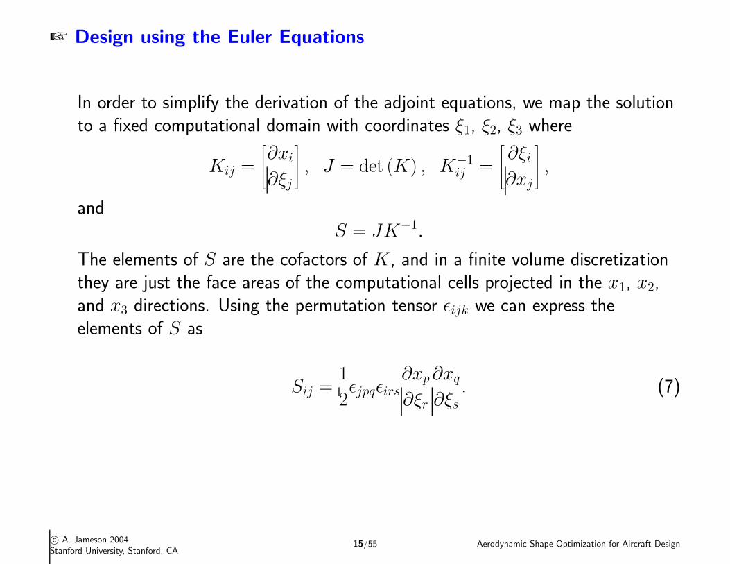
In order to simplify the derivation of the adjoint equations, we map the solutionto a fixed computational domain with coordinates ξ1, ξ2, ξ3 where
Kij =
∂xi∂ξj
, J = det (K) , K−1
ij =
∂ξi∂xj
,
andS = JK−1.
The elements of S are the cofactors of K, and in a finite volume discretizationthey are just the face areas of the computational cells projected in the x1, x2,and x3 directions. Using the permutation tensor εijk we can express theelements of S as
Sij =1
2εjpqεirs
∂xp∂ξr
∂xq∂ξs
. (7)
c© A. Jameson 2004Stanford University, Stanford, CA
15/55 Aerodynamic Shape Optimization for Aircraft Design
+ Design using the Euler Equations
Then
∂
∂ξiSij =
1
2εjpqεirs
∂2xp∂ξr∂ξi
∂xq∂ξs
+∂xp∂ξr
∂2xq∂ξs∂ξi
= 0. (8)
Also in the subsequent analysis of the effect of a shape variation it is useful tonote that
S1j = εjpq∂xp∂ξ2
∂xq∂ξ3
,
S2j = εjpq∂xp∂ξ3
∂xq∂ξ1
,
S3j = εjpq∂xp∂ξ1
∂xq∂ξ2
. (9)
c© A. Jameson 2004Stanford University, Stanford, CA
16/55 Aerodynamic Shape Optimization for Aircraft Design
+ Design using the Euler Equations
Now, multiplying equation(3) by J and applying the chain rule,
J∂w
∂t+R (w) = 0 (10)
where
R (w) = Sij∂fj∂ξi
=∂
∂ξi(Sijfj) , (11)
using (8). We can write the transformed fluxes in terms of the scaledcontravariant velocity components
Ui = Sijuj
as
Fi = Sijfj =
ρUiρUiu1 + Si1pρUiu2 + Si2pρUiu3 + Si3p
ρUiH
.
c© A. Jameson 2004Stanford University, Stanford, CA
17/55 Aerodynamic Shape Optimization for Aircraft Design
+ Design using the Euler Equations
For simplicity, it will be assumed that the portion of the boundary thatundergoes shape modifications is restricted to the coordinate surface ξ2 = 0.Then equations for the variation of the cost function and the adjoint boundaryconditions may be simplified by incorporating the conditions
n1 = n3 = 0, n2 = 1, dBξ = dξ1dξ3,
so that only the variation δF2 needs to be considered at the wall boundary. Thecondition that there is no flow through the wall boundary at ξ2 = 0 is equivalentto
U2 = 0, so that δU2 = 0
when the boundary shape is modified. Consequently the variation of the inviscidflux at the boundary reduces to
δF2 = δp
0
S21
S22
S23
0
+ p
0
δS21
δS22
δS23
0
. (12)
c© A. Jameson 2004Stanford University, Stanford, CA
18/55 Aerodynamic Shape Optimization for Aircraft Design
+ Design using the Euler Equations
In order to design a shape which will lead to a desired pressure distribution, anatural choice is to set
I =1
2
∫
B (p− pd)2 dS
where pd is the desired surface pressure, and the integral is evaluated over theactual surface area. In the computational domain this is transformed to
I =1
2
∫∫
Bw(p− pd)
2 |S2| dξ1dξ3,
where the quantity|S2| =
√
S2jS2j
denotes the face area corresponding to a unit element of face area in thecomputational domain.
c© A. Jameson 2004Stanford University, Stanford, CA
19/55 Aerodynamic Shape Optimization for Aircraft Design
+ Design using the Euler Equations
In the computational domain the adjoint equation assumes the form
CTi
∂ψ
∂ξi= 0 (13)
where
Ci = Sij∂fj∂w
.
To cancel the dependence of the boundary integral on δp, the adjoint boundarycondition reduces to
ψjnj = p− pd (14)
where nj are the components of the surface normal
nj =S2j
|S2|.
c© A. Jameson 2004Stanford University, Stanford, CA
20/55 Aerodynamic Shape Optimization for Aircraft Design
+ Design using the Euler Equations
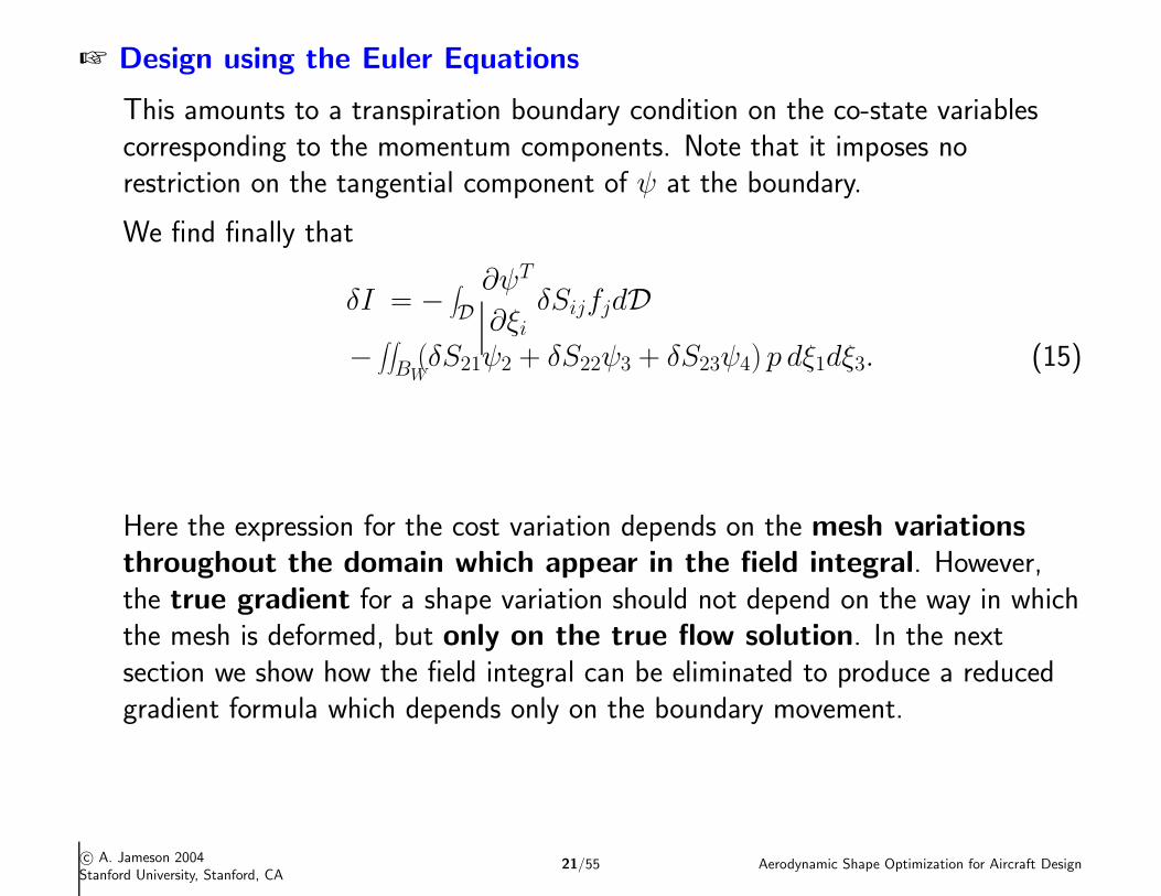
This amounts to a transpiration boundary condition on the co-state variablescorresponding to the momentum components. Note that it imposes norestriction on the tangential component of ψ at the boundary.
We find finally that
δI = −∫
D
∂ψT
∂ξiδSijfjdD
−∫∫
BW(δS21ψ2 + δS22ψ3 + δS23ψ4) p dξ1dξ3. (15)
Here the expression for the cost variation depends on the mesh variationsthroughout the domain which appear in the field integral. However,the true gradient for a shape variation should not depend on the way in whichthe mesh is deformed, but only on the true flow solution. In the nextsection we show how the field integral can be eliminated to produce a reducedgradient formula which depends only on the boundary movement.
c© A. Jameson 2004Stanford University, Stanford, CA
21/55 Aerodynamic Shape Optimization for Aircraft Design
+ The Reduced Gradient Formulation
Consider the case of a mesh variation with a fixed boundary. Then,
δI = 0
but there is a variation in the transformed flux,
δFi = Ciδw + δSijfj.
Here the true solution is unchanged. Thus, the variation δw is due to the meshmovement δx at each mesh point. Therefore
δw = ∇w · δx =∂w
∂xjδxj (= δw∗)
and since∂
∂ξiδFi = 0,
it follows that∂
∂ξi(δSijfj) = −
∂
∂ξi(Ciδw
∗) . (16)
It has been verified by Jameson and Kim∗ that this relation holds in the generalcase with boundary movement.
* Reduction of the Adjoint Gradient Formula in the Continuous Limit, A.Jameson and S. Kim, 41 st AIAA Aerospace Sciences
Meeting & Exhibit, AIAA Paper 2003-0040, Reno, NV, January 6-9, 2003.
c© A. Jameson 2004Stanford University, Stanford, CA
22/55 Aerodynamic Shape Optimization for Aircraft Design
+ The Reduced Gradient Formulation
Now∫
D φTδRdD =
∫
D φT ∂
∂ξiCi (δw − δw∗) dD
=∫
B φTCi (δw − δw∗) dB
−∫
D
∂φT
∂ξiCi (δw − δw∗) dD. (17)
Here on the wall boundary
C2δw = δF2 − δS2jfj. (18)
Thus, by choosing φ to satisfy the adjoint equation and the adjoint boundarycondition, we reduce the cost variation to a boundary integral which dependsonly on the surface displacement:
δI =∫
BWψT (δS2jfj + C2δw
∗) dξ1dξ3
−∫∫
BW(δS21ψ2 + δS22ψ3 + δS23ψ4) p dξ1dξ3. (19)
c© A. Jameson 2004Stanford University, Stanford, CA
23/55 Aerodynamic Shape Optimization for Aircraft Design
+ The Need for a Sobolev Inner Product in the Definition of theGradient
Another key issue for successful implementation of the continuous adjointmethod is the choice of an appropriate inner product for the definition of thegradient. It turns out that there is an enormous benefit from the use of amodified Sobolev gradient, which enables the generation of a sequence ofsmooth shapes. This can be illustrated by considering the simplest case of aproblem in the calculus of variations.
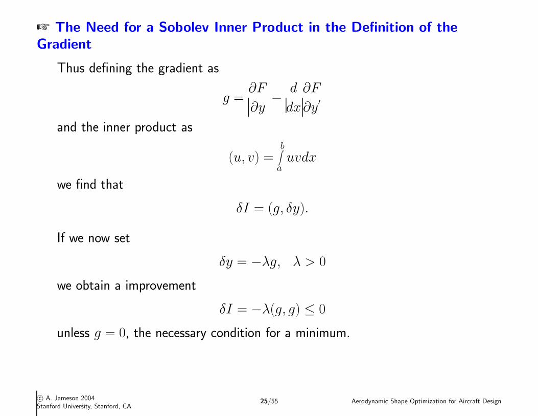
Suppose that we wish to find the path y(x) which minimizes
I =b
∫
aF (y, y
′)dx
with fixed end points y(a) and y(b). Under a variation δy(x),
δI =b
∫
a
∂F
∂yδy +
∂F
∂y′δy
′
dx
=b
∫
a
∂F
∂y−
d
dx
∂F
∂y′
δydx
c© A. Jameson 2004Stanford University, Stanford, CA
24/55 Aerodynamic Shape Optimization for Aircraft Design
+ The Need for a Sobolev Inner Product in the Definition of theGradient
Thus defining the gradient as
g =∂F
∂y−
d
dx
∂F
∂y′
and the inner product as
(u, v) =b
∫
auvdx
we find that
δI = (g, δy).
If we now set
δy = −λg, λ > 0
we obtain a improvement
δI = −λ(g, g) ≤ 0
unless g = 0, the necessary condition for a minimum.
c© A. Jameson 2004Stanford University, Stanford, CA
25/55 Aerodynamic Shape Optimization for Aircraft Design
+ The Need for a Sobolev Inner Product in the Definition of theGradient
Note that g is a function of y, y′, y
′′,
g = g(y, y′, y
′′)
In the well known case of the Brachistrone problem, for example, which calls forthe determination of the path of quickest descent between two laterallyseparated points when a particle falls under gravity,
F (y, y′) =
√
√
√
√
√
√
√
1 + y′2
y
and
g = −1 + y
′2 + 2yy′′
2(
y(1 + y′2))3/2
It can be seen that each step
yn+1 = yn − λngn
reduces the smoothness of y by two classes. Thus the computed trajectorybecomes less and less smooth, leading to instability.
c© A. Jameson 2004Stanford University, Stanford, CA
26/55 Aerodynamic Shape Optimization for Aircraft Design
+ The Need for a Sobolev Inner Product in the Definition of theGradient
In order to prevent this we can introduce a weighted Sobolev inner product
〈u, v〉 =∫
(uv + εu′v′)dx
where ε is a parameter that controls the weight of the derivatives. We nowdefine a gradient g such that
δI = 〈g, δy〉
Then we haveδI =
∫
(gδy + εg′δy
′)dx
=∫
(g −∂
∂xε∂g
∂x)δydx
= (g, δy)
where
g −∂
∂xε∂g
∂x= g
and g = 0 at the end points. Thus g can be obtained from g by a smoothingequation. Now the step
yn+1 = yn − λngn
gives an improvementδI = −λn〈gn, gn〉
but yn+1 has the same smoothness as yn, resulting in a stable process.
c© A. Jameson 2004Stanford University, Stanford, CA
27/55 Aerodynamic Shape Optimization for Aircraft Design
+ Outline of the Design Process
The design procedure can finally be summarized as follows:
1. Solve the flow equations for ρ, u1, u2, u3, p.
2. Solve the adjoint equations for ψ subject to appropriate boundary conditions.
3. Evaluate G and calculate the corresponding Sobolev gradient G.
4. Project G into an allowable subspace that satisfies any geometric constraints.
5. Update the shape based on the direction of steepest descent.
6. Return to 1 until convergence is reached.
Sobolev Gradient
Gradient Calculation
Flow Solution
Adjoint Solution
Shape & Grid
Repeat the Design Cycleuntil Convergence
Modification
Figure 3: Design cycle
c© A. Jameson 2004Stanford University, Stanford, CA
28/55 Aerodynamic Shape Optimization for Aircraft Design
+ Computational Costs∗
Cost of Search Algorithm
Steepest Descent O(N 2) stepsQuasi-Newton O(N) stepsSmoothed Gradient O(K) steps(Note: K is independent of N)
Total Computational Cost of Design
Finite Difference Gradients+ Steepest Descent O(N 3)Finite Difference Gradients+ Quasi-Newton Search O(N 2)Adjoint Gradients+ Quasi-Newton Search O(N)Adjoint Gradients+ Smoothed Gradient Search O(K)
(Note: K is independent of N)
* Studies of Alternative Numerical Optimization Methods Applied to the Brachistrone Problem, A.Jameson and J. Vassberg,Computational Fluid Dynamics, Journal, Vol. 9, No.3, Oct. 2000, pp. 281-296
c© A. Jameson 2004Stanford University, Stanford, CA
29/55 Aerodynamic Shape Optimization for Aircraft Design
+ Two dimensional studies of transonic airfoil design
Attainable shock-free solutions for various shape optimized airfoils
0.7 0.71 0.72 0.73 0.74 0.75 0.76 0.77 0.78 0.79 0.8 0.81 0.82 0.83 0.84 0.850.2
0.3
0.4
0.5
0.6
0.7
0.8
0.9
1
1.1
Mach number
CL
KornDLBA−243RAE 2822J78−06−10G78−06−10G70−10−13W100W110Cast7GAWG79−06−10
c© A. Jameson 2004Stanford University, Stanford, CA
30/55 Aerodynamic Shape Optimization for Aircraft Design
+Pre
ssure
distrib
utio
nand
Mach
conto
urs
forth
eD
LBA-2
43
airfo
il
DL
BA
-243 DR
AG
RE
DU
CT
ION
M
AC
H 0.770 A
LPH
A -1.752
CL
0.7021 CD
0.0139 CM
-0.3026G
RID
384X64 N
DE
S 0 RE
S0.593E-03 G
MA
X 0.100E
-05
0.1E+01 0.8E+00 0.4E+00 -.2E-15 -.4E+00 -.8E+00 -.1E+01 -.2E+01 -.2E+01
Cp
+++ ++
++++++
++++
+++++++++++++++++++++++
++++++
++++++++++++++++++++++++++++++++++++++++++++++++++
+++++++++++++++++++++++++++++++++++ + + + + + + + + + + + + + + + + + + + + + + + + + + + + + + + + + + + + + + + + + + + + + + + + + + + + + + + + + + + + + + + + + + + + + + + + + + + + + + + + + + + + + + + + + + + + + + + + + + + + + + + + + + + + + + + + + + + + + + +++++++++ +
DL
BA
-243 DR
AG
RE
DU
CT
ION
M
AC
H 0.770 A
LPH
A -0.966
CL
0.7008 CD
0.0013 CM
-0.2196G
RID
384X64 N
DE
S 20 RE
S0.288E-02 G
MA
X 0.123E
-02
0.1E+01 0.8E+00 0.4E+00 -.2E-15 -.4E+00 -.8E+00 -.1E+01 -.2E+01 -.2E+01
Cp
+++++
++++++
++++
++++++++ + +++ + + + + +++++++++++
++++++++++++
++++++
++++++
+++++++
++++++++
+++++++++
+++++++++++++
+++++++++++++++++++++++++ + + + + + + + + + + + + + + + + + + + + + + + + + + + + + + + + + + + + + + + + + + + + + + + + + + + + ++++++++++++++++++++++++++++++++++++++++++++++++ + + + + + +++++++++++++++++++++++ +
Before
theredesign
After
theredesign
c©A.Jam
eson
2004
Stan
fordU
niversity,
Stan
ford,CA
31/55
Aero
dyn
amic
Shap
eO
ptim
ization
forAircraft
Desig
n
+ Transonic similarity rule: M and CL scale with thickness ratio
0 0.5 1 1.5 2 2.50
0.5
1
1.5
τ2/τ
1
M /
CL
MC
L
c© A. Jameson 2004Stanford University, Stanford, CA
32/55 Aerodynamic Shape Optimization for Aircraft Design
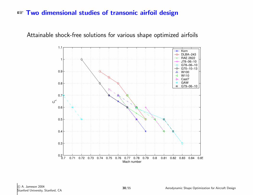
+ Planform and Aero-Structural Optimization
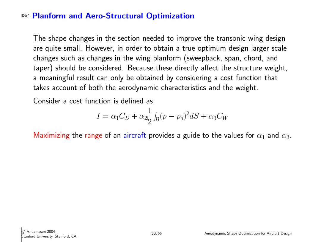
The shape changes in the section needed to improve the transonic wing designare quite small. However, in order to obtain a true optimum design larger scalechanges such as changes in the wing planform (sweepback, span, chord, andtaper) should be considered. Because these directly affect the structure weight,a meaningful result can only be obtained by considering a cost function thattakes account of both the aerodynamic characteristics and the weight.
Consider a cost function is defined as
I = α1CD + α2
1
2
∫
B(p− pd)2dS + α3CW
Maximizing the range of an aircraft provides a guide to the values for α1 and α3.
c© A. Jameson 2004Stanford University, Stanford, CA
33/55 Aerodynamic Shape Optimization for Aircraft Design
+ Choice of Weighting Constants
The simplified Breguet range equation can be expressed as
R =V
C
L
Dlog
W1
W2
where W2 is the empty weight of the aircraft.
With fixed VC
, W1, and L, the variation of R can be stated as
δR =V
C
δ
L
D
logW1
W2
+L
Dδ
logW1
W2
=V
C
−δD
D
L
Dlog
W1
W2
−L
D
δW2
W2
= −V
C
L
Dlog
W1
W2
δD
D+
1
logW1
W2
δW2
W2
Then,δR
R= −
δCDCD
+1
logW1
W2
δW2
W2
= −
δCDCD
+1
logCW1
CW2
δCW2
CW2
.
c© A. Jameson 2004Stanford University, Stanford, CA
34/55 Aerodynamic Shape Optimization for Aircraft Design
+ Choice of Weighting Constants (cont.)
Therefore minimizingI = CD + αCW ,
by choosing
α =CD
CW2log
CW1
CW2
, (20)
corresponds to maximizing the range of the aircraft.
c© A. Jameson 2004Stanford University, Stanford, CA
35/55 Aerodynamic Shape Optimization for Aircraft Design
+ Boeing 747 Euler Planform Results: Pareto Front
Test case: Boeing 747 wing-fuselage and modified geometries at the followingflow conditions M∞ = 0.87, CL = 0.42 (fixed), multiple α3
α1.
80 85 90 95 100 105 1100.038
0.040
0.042
0.044
0.046
0.048
0.050
0.052
CD (counts)
Cw
Pareto front
baseline
optimized section with fixed planform
X = optimized section and planform
maximized range
c© A. Jameson 2004Stanford University, Stanford, CA
36/55 Aerodynamic Shape Optimization for Aircraft Design
+ Boeing 747 Euler Planform Results: Sweepback, Span, Chord, and Section
Variations to Maximize Range
Baseline geometry —
Optimized geometry —
Geometry Baseline Optimized Variation(%)Sweep (deg) 42.1 38.8 - 7.8
Span (ft) 212.4 226.7 + 6.7Croot (ft) 48.1 48.6 + 1.0
Cmid (ft) 30.6 30.8 + 0.7Ctip (ft) 10.78 10.75 + 0.3
troot (in) 58.2 62.4 + 7.2tmid (in) 23.7 23.8 + 0.4ttip (in) 12.98 12.8 - 0.8
SYMBOL
SOURCE SYN88 DESIGN 19SYN88 DESIGN 0
ALPHA 1.930 2.189
CD 0.00872 0.01077
COMPARISON OF CHORDWISE PRESSURE DISTRIBUTIONSBOEING 747 WING-BODY
REN = 0.00 , MACH = 0.870 , CL = 0.420
Kasidit Leoviriyakit20:48 Thu
1 Jan 04COMPPLOT
JCV 1.13COMPPLOT
JCV 1.13COMPPLOT
JCV 1.13COMPPLOT
JCV 1.13COMPPLOT
JCV 1.13COMPPLOT
JCV 1.13COMPPLOT
JCV 1.13COMPPLOT
JCV 1.13COMPPLOT
JCV 1.13COMPPLOT
JCV 1.13
Solution 1 Upper-Surface Isobars
( Contours at 0.05 Cp )
0.2 0.4 0.6 0.8 1.0
-1.5
-1.0
-0.5
0.0
0.5
1.0
Cp
X / C 12.1% Span
0.2 0.4 0.6 0.8 1.0
-1.5
-1.0
-0.5
0.0
0.5
1.0
Cp
X / C 33.7% Span
0.2 0.4 0.6 0.8 1.0
-1.5
-1.0
-0.5
0.0
0.5
1.0
Cp
X / C 53.7% Span
0.2 0.4 0.6 0.8 1.0
-1.5
-1.0
-0.5
0.0
0.5
1.0
Cp
X / C 74.7% Span
0.2 0.4 0.6 0.8 1.0
-1.5
-1.0
-0.5
0.0
0.5
1.0C
pX / C
95.8% Span
ã CD is reduced from 107.7 drag counts to 87.2 drag counts (19.0%).
ã CW is reduced from 0.0455 (69,970 lbs) to 0.0450 (69,201 lbs) (1.1%).
c© A. Jameson 2004Stanford University, Stanford, CA
37/55 Aerodynamic Shape Optimization for Aircraft Design
+ Super B747
ã Design a new wing for the Boeing 747
ã Strategy
- Use the Boeing 747 fuselage
- Use a new planform (from the Planform Optimization result)
- Use new airfoil section (AJ airfoils)
- Optimized for fixed lift coefficient at three Mach numbers:
.78, .85, and .87
c© A. Jameson 2004Stanford University, Stanford, CA
38/55 Aerodynamic Shape Optimization for Aircraft Design
+ Super B747 at Mach .78: (Solid line = redesigned configuration), (Dash line = initial configuration)
B747 WING-BODY Mach: 0.780 Alpha: 2.683 CL: 0.449 CD: 0.01137 CM:-0.1369 Design: 30 Residual: 0.1710E-02 Grid: 257X 65X 49
Cl: 0.344 Cd: 0.05089 Cm:-0.1171 Root Section: 13.0% Semi-Span
Cp = -2.0
Cl: 0.569 Cd: 0.00036 Cm:-0.2516 Mid Section: 50.6% Semi-Span
Cp = -2.0
Cl: 0.453 Cd:-0.01561 Cm:-0.2117 Tip Section: 92.5% Semi-Span
Cp = -2.0
c© A. Jameson 2004Stanford University, Stanford, CA
39/55 Aerodynamic Shape Optimization for Aircraft Design
+ Super B747 at Mach .85: (Solid line = redesigned configuration), (Dash line = initial configuration)
B747 WING-BODY Mach: 0.850 Alpha: 2.220 CL: 0.449 CD: 0.01190 CM:-0.1498 Design: 30 Residual: 0.7857E-03 Grid: 257X 65X 49
Cl: 0.335 Cd: 0.05928 Cm:-0.1213 Root Section: 13.0% Semi-Span
Cp = -2.0
Cl: 0.572 Cd:-0.00217 Cm:-0.2602 Mid Section: 50.6% Semi-Span
Cp = -2.0
Cl: 0.462 Cd:-0.01878 Cm:-0.2213 Tip Section: 92.5% Semi-Span
Cp = -2.0
c© A. Jameson 2004Stanford University, Stanford, CA
40/55 Aerodynamic Shape Optimization for Aircraft Design
+ Super B747 at Mach .87: (Solid line = redesigned configuration), (Dash line = initial configuration)
B747 WING-BODY Mach: 0.870 Alpha: 1.997 CL: 0.449 CD: 0.01224 CM:-0.1590 Design: 30 Residual: 0.3222E-03 Grid: 257X 65X 49
Cl: 0.332 Cd: 0.06246 Cm:-0.1273 Root Section: 13.0% Semi-Span
Cp = -2.0
Cl: 0.574 Cd:-0.00334 Cm:-0.2674 Mid Section: 50.6% Semi-Span
Cp = -2.0
Cl: 0.464 Cd:-0.02110 Cm:-0.2222 Tip Section: 92.5% Semi-Span
Cp = -2.0
c© A. Jameson 2004Stanford University, Stanford, CA
41/55 Aerodynamic Shape Optimization for Aircraft Design
+ Drag Rise and Wing LD of Super B747
Drag Rise Wing LD
0.78 0.8 0.82 0.84 0.86 0.88 0.9 0.92100
120
140
160
180
200
220
240
260
280
Mach
CD
(cou
nts)
Drag rise at fixed CL
BaselineRedesign
0.78 0.8 0.82 0.84 0.86 0.88 0.9 0.9215
20
25
30
35
40
Mach
Win
g L/
D
Wing L/D vs. Mach at fixed CL
BaselineRedesign
- - - : Baseline
— : Redesigned
c© A. Jameson 2004Stanford University, Stanford, CA
42/55 Aerodynamic Shape Optimization for Aircraft Design
+ Drag Polars of Baseline and Super B747 at Mach .86
B747 WING-BODY
MACH 0.860 CD0 0.000
GRID 256X64X48
0.00 50.00 100.00 150.00 200.00 250.00 300.00
CD(counts)
0.0E
+00
0.1E
+00
0.2E
+00
0.3E
+00
0.4E
+00
0.5E
+00
0.6E
+00
0.7E
+00
0.8E
+00
CL
0.0E
+00
0.8E
+01
0.2E
+02
0.2E
+02
0.3E
+02
0.4E
+02
0.5E
+02
0.6E
+02
0.6E
+02
L/D
Solid line = Super B747, Dash line = Baseline B747
c© A. Jameson 2004Stanford University, Stanford, CA
43/55 Aerodynamic Shape Optimization for Aircraft Design
+ Drag Polars of Baseline and Super B747 at Mach .86
Boeing 747 Super B747CL CD CL CD
0.0045 94.3970 0.0009 76.94890.0500 82.2739 0.0505 67.80100.1000 74.6195 0.1005 64.61470.1501 72.1087 0.1506 65.50730.2002 73.9661 0.2006 69.48400.2503 79.6424 0.2507 76.00410.3005 88.7551 0.3008 84.98890.3507 101.5293 0.3509 95.61170.4009 118.0487 0.4010 106.96250.4512 141.2927 0.4510 121.71830.5014 177.0959 0.5010 141.86750.5516 228.1786 0.5512 175.25690.6016 298.0458 0.6014 222.5459
(CD in counts)
c© A. Jameson 2004Stanford University, Stanford, CA
44/55 Aerodynamic Shape Optimization for Aircraft Design
+ Comparison between Boeing 747 and Super B747
CL CD CWcounts counts
Boeing 747 .45 141.3 499(107.0 pressure, 34.3 viscous) (82,550 lbs)
Super B747 .50 141.9 427(104.8 pressure, 37.1 viscous) (70,620 lbs)
“Same drag at higher CL”
c© A. Jameson 2004Stanford University, Stanford, CA
45/55 Aerodynamic Shape Optimization for Aircraft Design
+ Super Wide-Body
c© A. Jameson 2004Stanford University, Stanford, CA
46/55 Aerodynamic Shape Optimization for Aircraft Design
+ Super Wide-Body at Mach .75: (Solid line = redesigned configuration), (Dash line = initial configuration)
SUPER WIDE-BODY Mach: 0.750 Alpha: 2.611 CL: 0.445 CD: 0.01243 CM:-0.1912 Design: 30 Residual: 0.1709E-02 Grid: 257X 65X 49
Cl: 0.389 Cd: 0.04637 Cm:-0.1437 Root Section: 13.4% Semi-Span
Cp = -2.0
Cl: 0.557 Cd: 0.00144 Cm:-0.2355 Mid Section: 50.8% Semi-Span
Cp = -2.0
Cl: 0.454 Cd:-0.01243 Cm:-0.2037 Tip Section: 92.5% Semi-Span
Cp = -2.0
c© A. Jameson 2004Stanford University, Stanford, CA
47/55 Aerodynamic Shape Optimization for Aircraft Design
+ Super Wide-Body at Mach .83: (Solid line = redesigned configuration), (Dash line = initial configuration)
SUPER WIDE-BODY Mach: 0.830 Alpha: 2.065 CL: 0.446 CD: 0.01329 CM:-0.2038 Design: 30 Residual: 0.3274E-03 Grid: 257X 65X 49
Cl: 0.383 Cd: 0.05328 Cm:-0.1521 Root Section: 13.4% Semi-Span
Cp = -2.0
Cl: 0.561 Cd:-0.00100 Cm:-0.2441 Mid Section: 50.8% Semi-Span
Cp = -2.0
Cl: 0.459 Cd:-0.01608 Cm:-0.2115 Tip Section: 92.5% Semi-Span
Cp = -2.0
c© A. Jameson 2004Stanford University, Stanford, CA
48/55 Aerodynamic Shape Optimization for Aircraft Design
+ Super Wide-Body at Mach .84: (Solid line = redesigned configuration), (Dash line = initial configuration)
SUPER WIDE-BODY Mach: 0.840 Alpha: 1.944 CL: 0.446 CD: 0.01358 CM:-0.2091 Design: 30 Residual: 0.2807E-03 Grid: 257X 65X 49
Cl: 0.382 Cd: 0.05451 Cm:-0.1557 Root Section: 13.4% Semi-Span
Cp = -2.0
Cl: 0.563 Cd:-0.00097 Cm:-0.2505 Mid Section: 50.8% Semi-Span
Cp = -2.0
Cl: 0.459 Cd:-0.01761 Cm:-0.2102 Tip Section: 92.5% Semi-Span
Cp = -2.0
c© A. Jameson 2004Stanford University, Stanford, CA
49/55 Aerodynamic Shape Optimization for Aircraft Design
+ Drag Rise and Wing LD of Super Wide-Body
Drag Rise Wing LD
0.74 0.76 0.78 0.8 0.82 0.84 0.86 0.88 0.9 0.92100
150
200
250
300
350
Mach
CD
(cou
nts)
Drag rise at fixed CL
BaselineRedesign
0.74 0.76 0.78 0.8 0.82 0.84 0.86 0.88 0.9 0.9210
15
20
25
30
35
40
Mach
Win
g L/
D
Wing L/D vs. Mach at fixed CL
BaselineRedesign
- - - : Baseline
— : Redesigned
c© A. Jameson 2004Stanford University, Stanford, CA
50/55 Aerodynamic Shape Optimization for Aircraft Design
+ Shape Optimization of Complete Business Jet Configuration
AIRPLANE DENSITY from 0.6250 to 1.1000
FALCON MACH 0.800 ALPHA 2.000 Z 6.00
CL 0.5351 CD 0.0157 CM -0.2097
NNODE 353887 NDES 0 RES0.287E-05
0.1E
+01
0.8E
+00
0.4E
+00
0.0E
+00
-.4E
+00
-.8E
+00
-.1E
+01
-.2E
+01
-.2E
+01
Cp
++++++++++++
++++
+++++++++++++++++++++++++++++++++
++++
++
+++
++
+
++
+++++++
+++++ +++ ++ +++ ++ ++ ++ +
++
+++
+++
+++ +++
++++++
++
FALCON MACH 0.800 ALPHA 2.000 Z 7.00
CL 0.5283 CD 0.0135 CM -0.2117
NNODE 353887 NDES 0 RES0.287E-05
0.1E
+01
0.8E
+00
0.4E
+00
0.0E
+00
-.4E
+00
-.8E
+00
-.1E
+01
-.2E
+01
-.2E
+01
Cp
+++++++++
++++++
++++++++++++++++++++++++++
++++
++
+++
+
+
+
+
+
+++++
+++++ +++ ++ +++ + +
+++ ++
+
+++
++
+ +++ ++++
+++
++
FALCON MACH 0.800 ALPHA 2.000 Z 8.00
CL 0.4713 CD 0.0092 CM -0.1915
NNODE 353887 NDES 0 RES0.287E-05
0.1E
+01
0.8E
+00
0.4E
+00
0.0E
+00
-.4E
+00
-.8E
+00
-.1E
+01
-.2E
+01
-.2E
+01
Cp
+++++++
+++
++
+++
++++++++++++++++++++++
++++
++
+++
+
+
+
++
++++++ ++ ++ +++
++++ +
+++
+
+
+
+++++ + ++
++++
++
Figure 4: Density contours for a business jet at M = 0.8, α = 2 and pressure distribution at 66,77,88 % of the wing
c© A. Jameson 2004Stanford University, Stanford, CA
51/55 Aerodynamic Shape Optimization for Aircraft Design
+ Shape Optimization of Complete Business Jet Configuration
AIRPLANE DENSITY from 0.6250 to 1.1000
FALCON MACH 0.800 ALPHA 2.298 Z 6.00
CL 0.5346 CD 0.0108 CM -0.1936
NNODE 353887 NDES 7 RES0.658E-03
0.1E
+01
0.8E
+00
0.4E
+00
0.0E
+00
-.4E
+00
-.8E
+00
-.1E
+01
-.2E
+01
-.2E
+01
Cp
++++++
+++++++++++++++++++++++++++++++++++++++++++++
+++++
++
++
+
+
+
++
+++++ +++++ +++ ++ +++ ++ ++ ++ +
+++
+++
++
+++
++
+++ ++++
++oooooo
ooooooooooooooooooooooooooooooooooooooooooo
oo
ooo
oo
o
oo
o
oo
oo
ooooo
ooooo ooo oo ooo oo oo o o ooo
oooo
oo
ooooo
ooo
ooooo
o
FALCON MACH 0.800 ALPHA 2.298 Z 7.00
CL 0.5417 CD 0.0071 CM -0.2090
NNODE 353887 NDES 7 RES0.658E-03
0.1E
+01
0.8E
+00
0.4E
+00
0.0E
+00
-.4E
+00
-.8E
+00
-.1E
+01
-.2E
+01
-.2E
+01
Cp
+++++
++++++++++++++++++++++++++++++++++++++
++
++
++++
+
+
+
+
+
+
++++++++ +++ ++ ++ + + +
+++++
+ ++++
++
+++
+
+++ + ++++ooooooo
ooooooooooooooooooooooooooooooooooo
o
oo
oo
ooo
o
o
o
o
o
ooooo
oooo ooo oo oo o o o ooooo o
ooo
ooo
ooo
oooo
ooo
oo
FALCON MACH 0.800 ALPHA 2.298 Z 8.00
CL 0.4909 CD 0.0028 CM -0.1951
NNODE 353887 NDES 7 RES0.658E-03
0.1E
+01
0.8E
+00
0.4E
+00
0.0E
+00
-.4E
+00
-.8E
+00
-.1E
+01
-.2E
+01
-.2E
+01
Cp
++++++
+++++++++++++++++++++++++++++
++++
++
+++++
+
+
+
++
++++++ ++ ++ +++ ++ ++ +
+++ ++
+
+++
++
++
++++ +
++ooooooooooooooooooooooooooooooooooooo
oo
o
o
o
ooo
o
o
o
oo
oo
oo oo oo oo ooo oo oo o ooo ooo
ooo
ooo
oo
oooo
oo
Figure 5: Density contours for a business jet at M = 0.8, α = 2 and pressure distribution at 66,77,88 % of the wing
c© A. Jameson 2004Stanford University, Stanford, CA
52/55 Aerodynamic Shape Optimization for Aircraft Design
+ Conclusions
ã An important conclusion of both the two- and the three-dimensional designstudies is that the wing sections needed to reduce shock strength or produceshock-free flow do not need to resemble the familiar flat-topped and aft-loadedsuper-critical profiles.
ã The section of almost any of the aircraft flying today, such as the Boeing 747 orMcDonnell-Douglas MD 11, can be adjusted to produce shock-free flow at achosen design point.
c© A. Jameson 2004Stanford University, Stanford, CA
53/55 Aerodynamic Shape Optimization for Aircraft Design
+ Conclusions
ã The accumulated experience of the last decade suggests that most existingaircraft which cruise at transonic speeds are amenable to a drag reduction of theorder of 3 to 5 percent, or an increase in the drag rise Mach number of at least.02.
ã These improvements can be achieved by very small shape modifications, whichare too subtle to allow their determination by trial and error methods.
ã When larger scale modifications such as planform variations or new wingsections are allowed, larger gains in the range of 5-10 percent are attainable.
c© A. Jameson 2004Stanford University, Stanford, CA
54/55 Aerodynamic Shape Optimization for Aircraft Design
+ Conclusions
ã The potential economic benefits are substantial, considering the fuel costs of theentire airline fleet.
ã Moreover, if one were to take full advantage of the increase in the lift to dragratio during the design process, a smaller aircraft could be designed to performthe same task, with consequent further cost reductions.
ã It seems inevitable that some method of this type will provide a basis foraerodynamic designs of the future.
c© A. Jameson 2004Stanford University, Stanford, CA
55/55 Aerodynamic Shape Optimization for Aircraft Design