Atmos. Chem. Phys., 12, 207–223, 2012www.atmos-chem-phys.net/12/207/2012/doi:10.5194/acp-12-207-2012© Author(s) 2012. CC Attribution 3.0 License.

AtmosphericChemistry

and Physics

Aerosol concentration and size distribution measured below, in, andabove cloud from the DOE G-1 during VOCALS-REx

L. I. Kleinman 1, P. H. Daum1, Y.-N. Lee1, E. R. Lewis1, A. J. Sedlacek III1, G. I. Senum1, S. R. Springston1, J. Wang1,J. Hubbe2, J. Jayne3, Q. Min4, S. S. Yum5, and G. Allen6

1Atmospheric Sciences Division, Brookhaven National Laboratory, Upton, New York, USA2Atmospheric Sciences & Global Change Division, Pacific Northwest National Laboratory, Richland, Washington, USA3Aerodyne Research Inc., Billerica, Massachusetts, USA4Atmospheric Sciences Research Center, State University of New York, Albany, New York, USA5Department of Atmospheric Sciences, Yonsei University, Seoul 120749, South Korea6Centre for atmospheric Science, University of Manchester, Manchester M13 9PL, UK

Correspondence to:L. I. Kleinman (kleinman@bnl.gov)

Received: 19 May 2011 – Published in Atmos. Chem. Phys. Discuss.: 21 June 2011Revised: 30 November 2011 – Accepted: 12 December 2011 – Published: 4 January 2012

Abstract. During the VOCALS Regional Experiment, theDOE G-1 aircraft was used to sample a varying aerosol envi-ronment pertinent to properties of stratocumulus clouds overa longitude band extending 800 km west from the Chileancoast at Arica. Trace gas and aerosol measurements are pre-sented as a function of longitude, altitude, and dew point inthis study. Spatial distributions are consistent with an up-per atmospheric source for O3 and South American coastalsources for marine boundary layer (MBL) CO and aerosol,most of which is acidic sulfate. Pollutant layers in the freetroposphere (FT) can be a result of emissions to the north inPeru or long range transport from the west. At a given alti-tude in the FT (up to 3 km), dew point varies by 40◦C withdry air descending from the upper atmospheric and moist airhaving a boundary layer (BL) contribution. Ascent of BLair to a cold high altitude results in the condensation andprecipitation removal of all but a few percent of BL wateralong with aerosol that served as CCN. Thus, aerosol vol-ume decreases with dew point in the FT. Aerosol size spectrahave a bimodal structure in the MBL and an intermediatediameter unimodal distribution in the FT. Comparing clouddroplet number concentration (CDNC) and pre-cloud aerosol(Dp >100 nm) gives a linear relation up to a number concen-tration of ∼150 cm−3, followed by a less than proportionalincrease in CDNC at higher aerosol number concentration.A number balance between below cloud aerosol and clouddroplets indicates that∼25 % of aerosol withDp>100 nmare interstitial (not activated). A direct comparison of pre-cloud and in-cloud aerosol yields a higher estimate. Artifacts

in the measurement of interstitial aerosol due to droplet shat-ter and evaporation are discussed. Within each of 102 con-stant altitude cloud transects, CDNC and interstitial aerosolwere anti-correlated. An examination of one cloud as a casestudy shows that the interstitial aerosol appears to have abackground, upon which is superimposed a high frequencysignal that contains the anti-correlation. The anti-correlationis a possible source of information on particle activation orevaporation.

1 Introduction

Satellite observations of cloud droplet effective radius indi-cate a gradient off the shore of Northern Chile. Accordingto MODIS retrievals from the Aqua satellite for the month ofOctober, average cloud droplet radius over the Pacific Oceanincreased from 8 to 14 µm from the coast to 1000 km offshore(Wood et al., 2007). This gradient is plausibly attributed toanthropogenic SO2 from point sources in Chile and Peru,subsequently oxidizded to aerosol sulfate.

Anthropogenic perturbations to marine stratocumulusclouds was one motivation for the VAMOS Ocean-Cloud-Climate-Atmosphere-Land Regional Experiment(VOCALS-REx or VOCALS, for short), an overview ofwhich is provided by Wood et al. (2011). The US DOEG-1 aircraft participated in the international collaborationdescribed by Wood et al. Aboard the G-1 were instrumentsfor in-situ measurements of cloud microphysics, aerosol

Published by Copernicus Publications on behalf of the European Geosciences Union.

208 L. I. Kleinman et al.: Aerosol concentration and size distribution

concentration, size distribution, and composition, gassesuseful as air mass tracers, and navigational and meteorolog-ical parameters. The sampling region of the G-1 extendedfrom Arica, Chile, 800 km west to 78◦ W mainly within arestricted latitude band between Arica at 18.35◦ S and 20◦ S.

Allen et al. (2011) have summarized meteorological con-ditions and the chemical composition of the boundary layerand free troposphere within one degree of 20◦ S between thecoast of Chile and 85◦ W, relying on aircraft measurementsfrom the United Kingdom BAe 146, NSF C130, and DOE G-1, supplemented by surface observations from the researchvessel Ronald H. Brown. Allen et al. (2011) provide mul-tiple comparisons between platforms which, in general, re-veals a high degree of consistency. Bretherton et al. (2010),relying principally on the C130, and BAe146 long range air-craft, provide a comprehensive synthesis of marine boundarylayer and free troposphere structure, clouds, and precipita-tion along the 20◦ S corridor. Further information on the ma-rine boundary layer and aerosol source attribution is given inRahn and Garreaud (2010) and Chand et al. (2010), respec-tively. In this study we provide a more complete treatmentof aerosol and trace gas measurements from the DOE G-1with emphasis on the longitudinal and vertical distributionof aerosol concentration and size distribution. Summary in-formation is provided on aerosol composition derived fromAerosol Mass Spectrometer (AMS) and Particle into Liq-uid Sampler (PILS) measurements, the primary descriptionof which will be contained in an article by Lee et al. (2011).

Data are presented for the entire field campaign, segre-gated into subsets according to longitude, altitude, dew pointtemperature (Td ), or whether measurements are below, in, orabove cloud. We find that dew point is a better indicator ofair mass type and origin than altitude and thus trends of tracegasses or aerosol as a function of dew point often show lessscatter than the same trends considered as a function of alti-tude.

The concentration and size distribution of interstitialaerosol are described. These are particles observed in-cloudthat either never grew into cloud droplets (i.e., were not acti-vated) or having been activated return to being aerosol parti-cles after cloud droplet evaporation. Properties of interstitialaerosol depend on many variables such as aerosol size andcomposition, cloud updraft velocity, and entrainment of dryair. Interstitial aerosols have been observed at mountain topsites (e.g. Hallberg et al., 1994; Martinsson et al., 1999; Hen-ning et al., 2002; Mertes et al., 2005) and from aircraft (e.g.Leaitch, 1986, 1996; Gillani et al., 1995; Wang et al., 2009).Results range from nearly complete activation of the accu-mulation mode to a low fractional activation leaving largerinterstitial aerosol particles than expected from an adiabaticcloud droplet activation model (Hallberg et al., 1994; Merteset al., 2005). Discrepancies could be due to external mix-tures, the type and quantity of organic aerosol constituents,or entrainment.

Table 1. Aerosol and cloud droplet instruments.

Instrument Primary function Dp range

CPC30251 total aerosol >3 nmCPC30101 total aerosol >10 nmSMPS (DMA)2 aerosol mobility size spectra 15–440 nmPCASP3 cabin 0.1–3 µmPCASP3 pylon 0.1–3 µmCAS2 cloud droplet 0.6–56 µmCIP2 drizzle 8–940 µmAMS4 aerosol composition 60–600 nmPILS5 aerosol composition <2 µmPSAP6 aerosol absorption <2 µm

1 TSI; 2 DMT Inc., model 3081 DMA and model 3010 condensation particle counterfor SMPS;3 PCASP-100X (Particle Measuring Systems, Inc., Boulder, CO) with SPP-200 electronics (Droplet measurement Technologies, Boulder, CO). Size range is nom-inal; 4 Aerodyne;5 Brookhaven National Laboratory;6 Radiance Research.

A simplifying feature of the VOCALS observations is thatbulk measurements of aerosol composition indicate a rela-tively uniform composition of easily activated particles. In-cloud sampling of aerosol is, however, problematic. Two ar-tifacts are discussed. Cloud droplet shatter is observed tocreate high concentrations of small particles (∼50 nm), witha size distribution extending into the accumulation moderange. The shatter contribution to total in-cloud aerosol be-comes minor at∼Dp>100–150 nm. Adiabatic heating in theG-1 aerosol inlet has the potential to evaporate cloud dropletscreating aerosol. A number-balance based comparison ofpre-cloud aerosol with CDNC yields an estimate that∼25 %of pre-cloud aerosol withDp>100 nm is interstitial. An es-timate of the interstitial aerosol based on in-cloud measure-ments, and therefore susceptible to artifact, is larger.

A more robust use of the in-cloud aerosol measurements isin examining the anti-correlation between aerosol interstitialconcentration and CDNC. One hundred and two cloud tran-sects were defined and an anti-correlation observed in each.One transect was selected as a case study and used to furtherillustrate aerosol and cloud droplet variability. A time seriesand high pass filter showed that the anti-correlation was car-ried in spikes and dips in aerosol concentration and LWC ona time scale of seconds or less, such as would be producedby an evaporating cloud droplet leaving behind an aerosolparticle.

2 Experimental

Aerosol properties are reported at ambient temperature andpressure. Local daylight savings times equal to UTC – 3 areused in this study. Data are archived athttp://iop.archive.arm.gov/arm-iop/0special-data/ASPCampaignspast/. (Sign inand follow menu to 2008VOCALS.), which uses UTC time.

Atmos. Chem. Phys., 12, 207–223, 2012 www.atmos-chem-phys.net/12/207/2012/

L. I. Kleinman et al.: Aerosol concentration and size distribution 209

2.1 Instruments

Aerosol and cloud instruments used in this study are listedin Table 1. The G-1 had its usual navigational and meteoro-logical package for measuring position, winds, temperature,and dew point (chilled mirror hygrometer)http://www.pnl.gov/atmospheric/programs/raf.stm. CO and O3 were usedas air mass tracers. CO was determined by VUV resonancefluorescence (Resonance Ltd., Barrie, ON, Canada). Ozonewas measured by a modified UV absorption detector (Model49-100, Thermo Electron Corporation, Franklin, MA). SO2measurements from a modified pulsed fluorescence detector(Model 43S, Thermo Electron Corporation, Franklin, MA)were typically below a 200 ppt limit of detection. Further in-formation on gas phase instruments used in VOCALS can befound in Springston et al. (2005) and Kleinman et al. (2007).

A forward facing two-stage diffuser aerosol inlet systemsupplied ambient air for aerosol instruments located insidethe cabin of the G-1 (Brechtel, 2003). Slowing down airfrom the G-1 speed of 100 m s−1 to a few m s−1 results in5◦C adiabatic heating. Droplet evaporation rates were cal-culated from the coupled heat and mass transfer equations inMcGraw and Liu (2006), (R. McGraw, personal communi-cation, 2011). Most droplets evaporate within one second.Less clear is the transit time of a cloud droplet through theinlet and plumbing inside the aircraft before impaction oc-curs. Our estimate is that these times scales are competitive.If evaporation occurs before impaction, aerosols so generatedwould mistakenly be classified as interstitial. Smaller clouddroplets may evaporate in the outside-cabin PCASP due toactive and passive heating applied over a residence time esti-mated to be 0.1–0.3 s (Strapp et al., 1992).

2.1.1 Aerosol composition

Aerosol composition was measured via an AMS and PILSand acidity determined by NH+4 to SO2−

4 ratio and conduc-tivity as described by Lee et al. (2011). They found thatnonrefractory, sub-micron size aerosol in the marine bound-ary layer had an average composition between (NH4)HSO4and H2SO4 with a 10–15 % admixture of organics. Acidicaerosol with this composition contains significant water evenat low relative humidity (RH) (Lee et al., 2011). Based on theE-AIM website,http://www.aim.env.uea.ac.uk/aim/aim.php,(Clegg et al., 1998) a solution consisting of 30 molal eachNH4HSO4 and H2SO4 is calculated to be in equilibrium atthe∼15 % RH used for particle size measurements. The den-sity of this solution is 1.56 g cm−3 at 298.15 K, insensitive totemperature (Clegg and Wexler, 2011). If an insoluble or-ganic component with density 1.2 g cm−3 comprises 10 % ofthe aerosol mass, then the volume growth factor at 15 % RH(calculated as the sum of the volumes of the solution and or-ganic component divided by the sums of the volumes of thesolutes and the organic component), is equal to 1.29, and theradial growth factor is 1.09.

2.1.2 Aerosol size distributions

Size distributions of aerosol particles in the Aitken and accu-mulation mode were quantified with one minute time resolu-tion using an SMPS (scanning mobility particle sizer) con-sisting of a cylindrical differential mobility analyzer (DMA)and a condensation particle counter. It is assumed that par-ticles are spherical so that mobility and geometric diame-ters are equal. Data were analyzed using the inversion al-gorithms described by Collins et al. (2002). A Nafion dryerupwind of the DMA reduced RH to 14 % (1σ = 2 %). In re-porting “dry” size distributions in this article, water of hy-dration at 14 % RH is not taken into account. Reportedparticle diameters are thus approximately 9 % larger than inthe dry state. In the case where there are few particles be-low the 15 nm lower limit of detection of the SMPS, the to-tal number of particles in the size range 15–440 nm shouldbe a good approximation for CN. Comparisons between theCPC3010 (Dp>10 nm) and the SMPS generally show agree-ment within 10 % for sampling periods without appreciableconcentrations of small particles.

Two Passive Cavity Aerosol Spectrometer (PCASP) unitswith SPP-200 electronics upgrade were used to measureaerosol with nominal diameter between 0.1 and 3 µm. OnePCASP was mounted on a pylon on the nose of the aircraftand the other located inside the cabin. In the data archive thetwo PCASPs are identified as units A and B. Midway throughthe program these units were switched, so that from the startof the program through 28 October, unit A was outside andunit B inside. From 29 October till the end of the VOCALScampaign, unit B was outside and unit A inside. The relativehumidity of air sampled by both PCASPs was decreased bythe use of deicing heaters which yields an increase in temper-ature, reported to be 10 to 20◦C (Strapp et al., 1992; Hallaret al., 2006; Snider and Petters, 2008). Cabin heat also con-tributed to the drying of aerosol measured inside the aircraft.

PCASPs were calibrated with PSL particles with a refrac-tive index (RI) of 1.59. For the data archive, a Mie scat-tering code was used to generate data at RI = 1.55, a valueslightly more representative of continental aerosol. For thisstudy, a second Mie scattering calculation was used to ad-just size bins to an RI of H2SO4 (1.41). This is close tothe volume weighted refractive index determined from non-refractory components of sub micrometer size aerosol mea-sured by the AMS (RI = 1.46). Addition of retained water(RI = 1.33) results in a lower refractive index, close to 1.41.

Comparisons were made between aerosol volume deter-mined by the SMPS and the two PCASPs. In order to matchsize ranges, volumes are calculated forDp between 0.11 and0.44 µm. A linear regression of PCASP A volume vs. SMPSvolume had a slope of 0.84 andr2 = 0.91; for PCASP Bthe slope andr2 were 0.98 and 0.93, respectively. Agree-ment is well within the 30 % uncertainty limits typicallycited for PCASP and SMPS volume measurements. Volumes

www.atmos-chem-phys.net/12/207/2012/ Atmos. Chem. Phys., 12, 207–223, 2012

210 L. I. Kleinman et al.: Aerosol concentration and size distribution

determined by PCASP A and B vary by only a few percentaccording to which unit is inside or outside of the aircraft.

PCASP and SMPS number distributions differed, primar-ily due to a low detection efficiency of small particles in thePCASP (Dp<160 nm), which was confirmed only recentlyin a post-flight calibration of PCASP A. PCASP size dis-tributions were adjusted to match those from the SMPS. Aset of global adjustment factors to be applied to all PCASPdata were determined by performing a linear regression be-tween the SMPS and PCASP A and PCASP B for 15 sizebins. All non-cloud data were used for these regressions. Totest the normalization procedure, plots were made of PCASPvs. SMPS number concentration integrated over the overlapsize range 110–440 nm (not shown). A least squares regres-sion yields slopes of 0.95 and 0.96 for PCASP A and B vs.SMPS, respectively, both with anr2 of 0.85. By constructionslopes should be close to unity. Scatter in the number com-parisons is a measure of how well a single set of adjustmentfactors works in the differing environments encountered over16 flights. Normalization resulted in an increase of total par-ticle concentration by 41 % and 18 % from PCASP A andPCASP B, respectively.

By adjusting the PCASP data, we are relying on the SMPSas providing an intrinsically more accurate size distribution.The adjustment procedure allows for the determination ofnumber concentrations and size distributions with 1s timeresolution using PCASP data which on average agrees withthe SMPS. Fast response aerosol number concentrations willprove useful in examining the anti-correlation between clouddroplets and interstitial aerosol.

2.1.3 Cloud microphysics

Cloud droplet number concentration (CDNC) was de-termined via a Cloud and Aerosol Spectrometer (CAS)probe manufactured by Droplet Measurement Technologies(DMT). Results were integrated over a diameter range be-tween 2.5 and 50 µm. Cloud liquid water content (LWC) wasmeasured with a Particle Volume Monitor (PVM, Gerber etal., 1994) and checked against a hot wire detector. Drizzleconcentration was determined from a DMT Cloud ImagingProbe (CIP) which together with the CAS and hot wire de-tector are packaged together as a Cloud, Aerosol, and Pre-cipitation Spectrometer (CAPS), mounted on a pylon off thenose of the G-1. Data has been archived at 0.1, 1, and 10 Hz,and is available on request at 40 and in some cases 200 Hz.

2.2 Flights

Figure 1 shows the 3-D sampling region of the G-1 during 16of 17 research flights. An electrical failure on 18 Oct. limiteddata collection and that flight is not used in this study. Instru-ment status and flight times are tabulated in spreadsheet for-mat on the same ftp site as the data. Flight duration was ap-

Fig. 1. Ground track of G-1 color coded by CO concentration. Aportion of one flight south of−20.5 latitude not shown.

proximately 4 h. Thirteen of 16 flights started between 08:57and 10:20 (11:57 and 13:20 UTC).

Flight objectives were to determine the horizontal and ver-tical variability of cloud and aerosol properties. The rangeof the G-1 allowed for sampling between Arica at 70.3◦ Wout over the Pacific to 78◦ W, an E-W distance of 800 km.Vertical sampling was primarily done via multiple transectsat different altitudes or ascents and descents through clouds,and less often by porposing between cloud and above-cloudregions.

A typical flight track designed to sample longitudinal vari-ations in cloud and aerosol properties is shown in Fig. 2.Because clouds thinned and sometimes disappeared due pri-marily to solar heating as the day progressed, the out boundleg was usually devoted to cloud sampling and the inboundleg to sampling in the boundary layer below cloud height.In order to examine interstitial aerosol, 102 constant altitudetransects were identified in which the maximum liquid watercontent (LWC) was at least 0.1 g m−3. Often there were mul-tiple transects in a single cloud separated by a step changein altitude of order tens of m or greater. For many transectsclouds were broken or occupied only a portion of the tran-sect. One cloud on Flight 081028a (Fig. 2) is singled out asa case study to illustrate the anti-correlation between clouddroplet number concentration and interstitial aerosol foundin all 102 cloud transects.

As indicated in Fig. 3, aerosol number concentration mea-sured by SMPS was nearly the same on outbound and in-bound legs, even though below-cloud measurements at a par-ticular longitude could be separated by 500 m in altitude andmore than 3 h in time (compare with Fig. 2). There are iso-lated occurrences in other flights of transects within 100 mof cloud base and in the mid to bottom MBL, in general in-dicating well mixed aerosol below cloud base. On average,

Atmos. Chem. Phys., 12, 207–223, 2012 www.atmos-chem-phys.net/12/207/2012/

L. I. Kleinman et al.: Aerosol concentration and size distribution 211

Fig. 2. Longitude-altitude cross section of flight track for 081028acolor coded for cloud liquid water content in g m−3. Cloud at−75.2◦ W longitude is used to illustrate anti-correlation betweencloud droplets and interstitial aerosol.

Fig. 3. Below cloud level SMPS measurement of number of parti-cles withDp>75 nm.

pre-cloud aerosol can be represented by low altitude sam-ples collected at the same longitude. In addition, becausehorizontal gradients in composition are small, we allow airwithin 15 km of a cloud to be called pre-cloud. These ap-proximations lead to scatter in relations between cloud andpre-cloud properties.

There were 3 intercomparison flights between the G-1 andC130, BAe-146 and Twin Otter that yielded data on LWCand CDNC (from a CDP or CAS probe). Results are sum-marized in Table 2. Intercomparisons were conducted witha several minute time separation between aircraft. Small dif-ferences in location, especially altitude, had a large influenceon LWC. More significant are differences in CDNC wherethe G-1 values have to be reduced by 10, 17 and 38 % tomatch the C130, TO, and BAe146, respectively. Althoughthe comparison with the BAe146 is based on a short sam-ple through broken clouds, a particle balance between belowcloud and in-cloud is consistent with the G-1 CDNC beingapproximately 20 % too high – of the same order as pub-lished estimates of measurement uncertainty (Fountoukis etal., 2007). This factor also agrees with inter-platform differ-ences in CDNC vs. longitude (not shown).

3 Results

Source regions for aerosol and trace gases have been ana-lyzed by Allen et al. (2011) and Bretherton et al. (2010) bymeans of back trajectories calculated for marine boundarylayer (MBL) at 950 hPa and free troposphere (FT) at 850 hPastarting from 20◦ S at distances from the shore varying from70.5◦ W to 90◦ W. Much of this work is pertinent to the lon-gitudinal and vertical pollutant distribution measured by theG-1. Allen et al. (2011) and Bretherton et al. (2010) foundthat pollutants in the near coastal MBL could be explainedby low altitude winds from the S and SE that intersectedthe Chilean coast. Trajectories terminating further offshorewhere pollution levels are lower tend to remain off shore,missing coastal emission sources. FT back trajectories weremore diverse. In one population, descending air from the di-rection of Australia and South Asia carried pollutants to theVOCALS region. Another category of FT trajectory preva-lent between the coast and 75◦ W were northerlies from Pe-ruvian coastal regions. A contribution to the FT consisting ofreturn coastal flow from the MBL is hypothesized by Allenet al. (2011) based on instances with high humidity and lowO3.

3.1 Spatial distributions

Data have been segregated into marine boundary layer, pre-cloud, in-cloud, and free tropospheric subsets, as defined inTable 3. Except when used in a general sense, the term“MBL” refers to non-cloud air below 800 m altitude. Theparticular definition of MBL can be recognized as it refersto, e.g. a region in which an average concentration or sizedistribution has been calculated. Below-cloud is that partof the data within the MBL (used as a general term) thatis defined as being below clouds that were encountered onascents and descents. Pre-cloud air is an approximation tothe air actually ingested into a cloud. Because there are onlya few instances of flight transects within cloud followed orpreceded by a flight segment within∼100 m of cloud base,several approximations are used in defining pre-cloud air, asgiven in Table 3 and described in Sect. 2.2. Clouds were lo-cated primarily between 800 and 1200 m altitude with cloudbase and inversion height increasing with distance from theshore (Rahn and Garreaud, 2010; Bretherton et al., 2010).

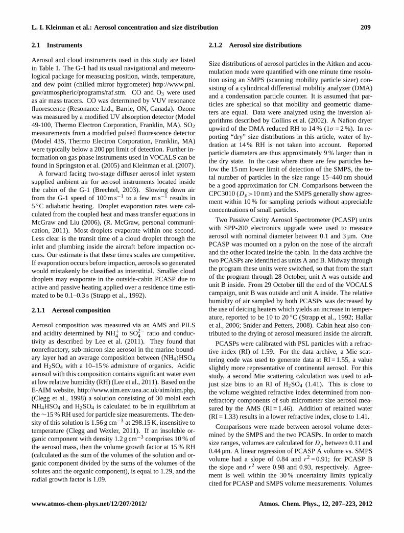
Figure 4 shows frequency distributions of sub-micrometeraerosol number and volume concentration and CO and O3mixing ratio as a function of longitude for the below cloudlayer. Aerosol number concentration and volume decrease2.3 and 3.6-fold, respectively between 70◦ and 75◦ W, thedifference between number and volume appearing in theaerosol size distributions, presented below. There is a mono-tonic decrease in CO between 70◦ and 75◦ W totaling 10 ppb,while O3 increases by 9 ppb and continues to increase west of75◦ to the limit of our sampling at 78◦ W. In contrast, CO andaerosol number and volume do not have a significant zonal

www.atmos-chem-phys.net/12/207/2012/ Atmos. Chem. Phys., 12, 207–223, 2012

212 L. I. Kleinman et al.: Aerosol concentration and size distribution

Table 2. Cloud sampling intercomparisons.

Platform Date G-1 Other aircraft

CDNC LWC Time1 CDNC LWC Time1

TO 26 Oct 402 0.16 10:47–10:52 335 0.14 10:54–11:04C130 04 Nov 226 0.10 11:28–11:35 203 0.16 11:25–11:33BAe-146 12 Nov 47.32 0.00652 12:49–12:56 29.3 0.0095 12:45–12:51

1 rounded off to nearest minute.2 Maximum values∼400 cm−3, 0.1 g m−3, in-cloud for∼1 min.

Table 3. Definition of atmospheric layers.

Variable1 Data Subset

marine boundary layer pre-cloud in-cloud above-cloudAltitude (m) <800 below and within 15 km of cloud >600 >1200RH ( %) n/a <90 n/a n/aTheta (◦C) n/a n/a n/a >22LWC (g m−3) <0.01 <0.01 >0.02, LWCavg>0.05 <0.01

1 Condition applies to each 1s time period within averaging time, except for LWCavg which is an average value over a 1 minute SMPS scan.

gradient west of 75◦. Median concentrations in the free tro-posphere are also given in Fig. 4. Concentrations are highestnear the coast except for O3. Relative to the marine bound-ary layer, CO and especially O3 have a greater concentrationin the free troposphere. Particle volume decreases several-fold with altitude but number concentration decreases onlymarginally, a result consistent with size distributions shownin a following section. The broad covariance between MBLand FT aerosol and trace gases suggest coupling betweenthese atmospheric layers.

Even though the sampling region of the G-1 was primarilynorth of the 20◦ S corridor reported on by Allen et al. (2011),there is excellent agreement in longitudinal structure in theMBL and FT for the 3 quantities that can be directly com-pared: O3, CO, and CN (10 nm lower limit from CPC 3010on BAe146, 15 nm from SMPS on G-1). SO2 concentra-tions were below our detection limit of∼0.2 ppb except for afew near coast measurements, not surprising in a cloud cov-ered MBL where there is opportunity for aqueous phase re-action with H2O2. With a more sensitive instrument, Allen etal. (2011) report mean SO2 concentrations of 20–30 ppt, withhigher values near the coast and concentrations approach-ing 1/2 ppb in a few discrete layers at 2–3 km altitude. Thegeneral picture based on longitudinally dependent SO2 andaerosol sulfate measurements is that even near the shore,within the MBL, air masses had a high sulfate to SO2 molarratio indicating that with respect to sulfur theses air masseswere aged.

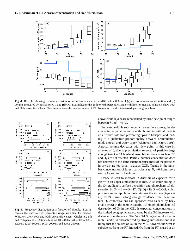
Frequency distributions as a function of altitude have beenconstructed by dividing the data set into altitude bins asshown in Fig. 5. Data points in and out of clouds are in-

cluded for CO and O3, but points with LWC>0.01 g m−3 areexcluded for aerosol number and volume. Because samplesare not uniformly distributed in longitude or altitude, thereare biases in constructing these vertical profiles. As can beseen from Fig. 1, high altitude points are primarily east of74◦. Also, according to Fig. 5f, data points between 400–800 m are closer to the shore than those in the lower altitudebin (100–400 m) thereby accounting for aerosol volume in-creasing with altitude in the two low altitude bins (Fig. 5b).The vertical structure shown in Fig. 4, in general, appearsmore pronounced than that shown in Fig. 5. This is partlyan artifact caused by sampling inhomogeneities mentionedabove. There is also a real difference in the data sets as theFT data in Fig. 4 incorporates the requirement that potentialtemperature,θ , exceed 22◦C, a constraint that insures sepa-ration between below and above cloud aerosol size spectra.

Figure 5e shows that in each of the three above cloud al-titude bins, dew point varies by about 40◦C, indicating thatat a given altitude in the FT air masses with very differenthistories are being sampled. As dew point is controlled bythe maximum altitude to which an air parcel is lifted, lowerdew points indicate air masses that subsided from the middleor upper troposphere, whilst higher dew points indicate airmasses that have a boundary layer origin. The associationbetween dew point and air mass origin prompts us to exam-ine aerosol and trace gas concentration as a function of dewpoint in Fig. 6. A qualitative correspondence between layersdefined according to dew point and those defined accordingto altitude is that the below-cloud part of the MBL corre-sponds to the two bins with highest dew point (> 10◦C), thecloud layer has dew point between 6 and 10◦C, and the three

Atmos. Chem. Phys., 12, 207–223, 2012 www.atmos-chem-phys.net/12/207/2012/

L. I. Kleinman et al.: Aerosol concentration and size distribution 213

Fig. 4. Box plot showing frequency distribution of measurements in the MBL below 800 m of(a) aerosol number concentration and(b)volume measured by SMPS,(c) O3, and(d) CO. Box indicates the 25th to 75th percentile range with line for median. Whiskers show 10thand 90th percentile values. Blue lines indicate the median values of FT observation divided into two degree longitude bins.

Fig. 5. Frequency distribution as a function of altitude. Box in-dicates the 25th to 75th percentile range with line for median.Whiskers show 10th and 90th percentile values. Circles are 5thand 95th percentile. Altitude bins are 100–400 m, 400–800 m, 800–1200 m, 1200–1600 m, 1600–2000 m, and above 2000 m.

above cloud layers are represented by three dew point rangesbetween 6 and−40◦C.

For water soluble substances with a surface source, the de-crease in temperature and specific humidity with altitude isan effective cold trap preventing upward transport and lead-ing to a qualitative proportionality between accumulationmode aerosol and water vapor (Kleinman and Daum, 1991).Aerosol volume decreases with dew point, in this case bya factor of 6, due to precipitation removal of particles largeenough to act as CCN whilst insoluble substances such as COand O3 are not affected. Particle number concentration doesnot decrease to the same extent because most of the particlesin dry air are too small to act as CCN. Trends in the num-ber concentration of larger particles, sayDp>0.1 µm, morenearly follow aerosol volume.

Ozone is seen to increase in drier air as expected for agas with an upper atmospheric source. Also contributing tothe O3 gradient is surface deposition and photochemical de-struction by O3 + hν→O (1D); O(1D) + H2O→2 OH, whichproceeds more rapidly in moist air near the surface (Ayers etal., 1992). Given a long enough residence time, near sur-face O3 concentrations can approach zero as seen by Kleyet al. (1996) in the remote Pacific. Although photochemicaldestruction of O3 in the MBL is expected, concentrations inthe limited geographic area covered by the G-1 increase withdistance from the coast. The VOCALS region, unlike the re-mote Pacific, is characterized by strong subsidence and it islikely that the source of O3 in the MBL towards the west issubsidence from the FT. Indeed, O3 from the FT is used as an

www.atmos-chem-phys.net/12/207/2012/ Atmos. Chem. Phys., 12, 207–223, 2012

214 L. I. Kleinman et al.: Aerosol concentration and size distribution

Fig. 6. Frequency distribution as a function of dew point. Boxplot format same as in Fig. 5. Dew point bins are 16 to 12◦C,12 to 10◦C, 10 to 6◦C, 6 to 0◦C, 0 to−20◦C, −20 to −40◦C.Qualitatively, the first 2 bins are below cloud, the third bin in thecloud layer, and the driest 3 bins above cloud.

inert tracer to quantify cloud top entrainment (e.g. Faloona etal., 2005). Aerosol particles will be entrained as a componentof FT O3 containing air. Although large particles in the FTare fewer than in the MBL (Sect. 3.2, following), they can, asshown by Clarke et al. (1996, 1997), provide CCN to replacethose lost by drizzle – a process of particular importance inthe drizzled out Pocket of Open Cell (POC) regions furtherwest than the G-1 sampled (Wood et al., 2011).

In the MBL, CO is anti-correlated with O3 consistent withthe oppositely directed east-west trends shown in Figs. 4cand d. Emission sources are located on land which lendssome logic to CO concentrations being highest near the shorebut does not address the near-shore O3 which not only is lowbut is also anticorrelated with CO. CO-O3 anticorrelationsof the type observed in winter by Parrish et al. (1998) donot seem relevant in the low NOx VOCALS region. Allenet al. (2011) suggest the possible effects of fresh emissionsbut also note that a transport process may be responsible. Anexplanation for the low near-shore O3 may have to await pro-cess analysis of chemical transport model results (Yang et al.,2011).

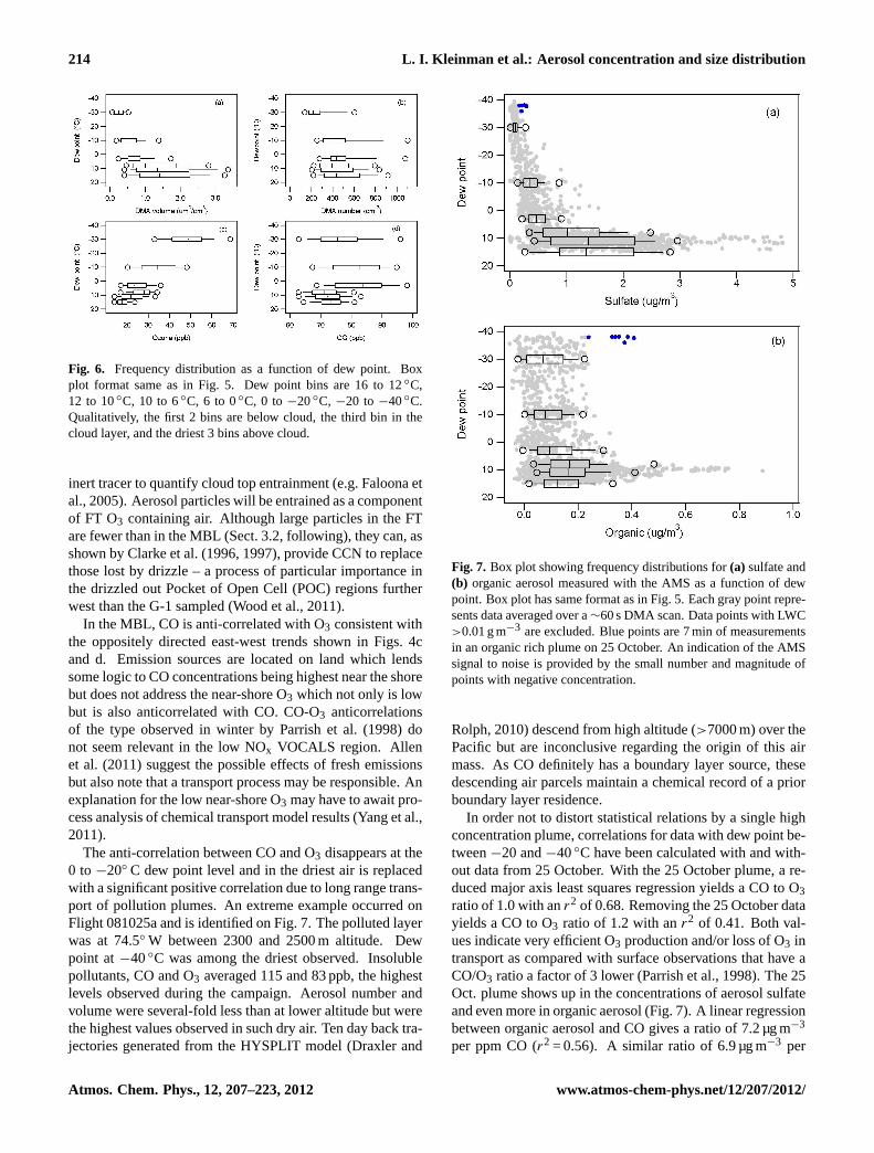
The anti-correlation between CO and O3 disappears at the0 to −20◦ C dew point level and in the driest air is replacedwith a significant positive correlation due to long range trans-port of pollution plumes. An extreme example occurred onFlight 081025a and is identified on Fig. 7. The polluted layerwas at 74.5◦ W between 2300 and 2500 m altitude. Dewpoint at−40◦C was among the driest observed. Insolublepollutants, CO and O3 averaged 115 and 83 ppb, the highestlevels observed during the campaign. Aerosol number andvolume were several-fold less than at lower altitude but werethe highest values observed in such dry air. Ten day back tra-jectories generated from the HYSPLIT model (Draxler and

Fig. 7. Box plot showing frequency distributions for(a) sulfate and(b) organic aerosol measured with the AMS as a function of dewpoint. Box plot has same format as in Fig. 5. Each gray point repre-sents data averaged over a∼60 s DMA scan. Data points with LWC>0.01 g m−3 are excluded. Blue points are 7 min of measurementsin an organic rich plume on 25 October. An indication of the AMSsignal to noise is provided by the small number and magnitude ofpoints with negative concentration.

Rolph, 2010) descend from high altitude (>7000 m) over thePacific but are inconclusive regarding the origin of this airmass. As CO definitely has a boundary layer source, thesedescending air parcels maintain a chemical record of a priorboundary layer residence.

In order not to distort statistical relations by a single highconcentration plume, correlations for data with dew point be-tween−20 and−40◦C have been calculated with and with-out data from 25 October. With the 25 October plume, a re-duced major axis least squares regression yields a CO to O3ratio of 1.0 with anr2 of 0.68. Removing the 25 October datayields a CO to O3 ratio of 1.2 with anr2 of 0.41. Both val-ues indicate very efficient O3 production and/or loss of O3 intransport as compared with surface observations that have aCO/O3 ratio a factor of 3 lower (Parrish et al., 1998). The 25Oct. plume shows up in the concentrations of aerosol sulfateand even more in organic aerosol (Fig. 7). A linear regressionbetween organic aerosol and CO gives a ratio of 7.2 µg m−3

per ppm CO (r2 = 0.56). A similar ratio of 6.9 µg m−3 per

Atmos. Chem. Phys., 12, 207–223, 2012 www.atmos-chem-phys.net/12/207/2012/

L. I. Kleinman et al.: Aerosol concentration and size distribution 215

ppm CO is obtained without data from 25 October. Thesevalues are an order of magnitude lower than found in pollutedboundary layer air masses after about one day of photochem-ical processing (Kleinman et al., 2008), indicating precipita-tion removal of aerosol.

In addition to the CO plumes observed in the driest airthere are observations of high CO (>80 ppb) concentration,located over a range of altitudes with dew points between0 and 6◦ C (i.e. in the bin just above the cloud layer). COin these cases is anti-correlated with O3. HYSPLIT backtrajectories intercept or come close to the Peruvian coast inagreement with wind measurements presented by Brether-ton et al. (2010) and Rahn and Garreaud (2010). Brether-ton et al. (2010) note that heating of the Andean slope mixesmoisture into a layer that becomes the lower free tropospherewhen advected over the Pacific. High concentrations of COin the moist above cloud layer are further evidence of theupward mixing of continental boundary layer air. The nextdriest bin in Fig. 6 also has data points with high CO. Herethe anti-correlation between CO and O3 has changed into alack of correlation.

Concentrations of aerosol sulfate and organics both de-crease with altitude (Lee et al., 2011) or dew point (Fig. 7).There is a selective reduction in aerosol sulfate in dry airwhich could reflect a greater solubility in cloud droplets andpropensity for wet removal, relative to organics, and/or a dif-ferent mixture of sources affecting boundary layer and freetropospheric air. Whereas the organic to sulfate ratio is∼0.1in the marine boundary layer it increases to above 0.5 in thedriest air and is greater than 1 in the plume encountered on25 October. Absorption measurements were examined forinformation on light absorbing carbon aerosol. Except forisolated plumes and areas near land, aerosol absorption wastoo low to reliably quantify with a median value of 0.6 Mm−1

in the boundary layer and 0.4 Mm−1 above.

3.2 Aerosol size distribution

Aerosol size distributions measured with the SMPS areshown as a function of longitude in Fig. 8 for the belowcloud layer and free troposphere. Below cloud aerosol hasa characteristic two mode structure separated by a minimum.As described by Hoppel et al. (1986) this minimum is theresult of a selective activation of larger aerosol particles inthe cloud forming process. Aqueous phase chemistry, princi-pally the oxidation of SO2 to sulfate adds solute mass. Uponcloud evaporation, larger aerosol particles that had been acti-vated create an accumulation-size mode (sometimes calleda droplet mode) that is distinct from the smaller aerosolparticles that have not increased in mass by aqueous phasechemistry. Composition measurements reported by Lee etal. (2011) show that sub micron size aerosol is primarily par-tially neutralized H2SO4, consistent with a formation routeby aqueous phase oxidation of SO2. It would be expectedthat the droplet mode contains a higher ratio of sulfate to or-

Fig. 8. Aerosol size distribution measured with SMPS(a) in theMBL below 800 m and(b) above cloud layer.

ganics than the Aitken mode. This, however, could not betested using AMS size distributions because the volume ofthe Aitken mode was too small to quantify. With increas-ing distance from the shore, Fig. 8 shows that the dropletmode contains an increasing fraction of the total aerosol. Atthe same time, the droplet mode becomes narrower with adecreasing proportion of larger particle (Dp>300 nm). Thedroplet mode size is nearly invariant (Dp = 160-185 nm) butthe Hoppel minimum diameter and the Aitken mode sizemove to lower values. A possible mechanism for the move-ment of the Hoppel minimum diameter and Aitken mode toa smaller size is that aerosol concentrations are lower furtherfrom the coast, which in the presence of a fixed vertical ve-locity results in smaller particles being activated. In contrast,free tropospheric aerosol is predominately unimodal with amode size between that for Aitken and accumulation modesobserved in the MBL.

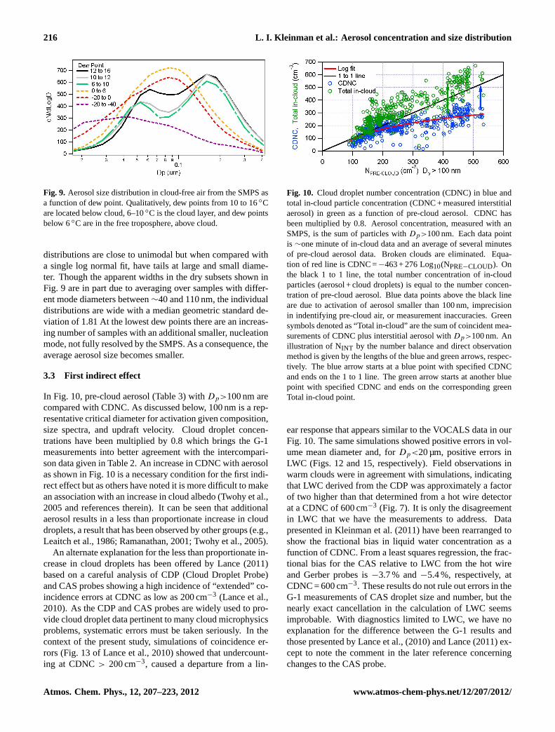
Size distributions of aerosol particles as functions of dewpoint are shown in Fig. 9. Particles in the boundary/cloudylayer with Td>6◦C are seen to have a bimodal distributioncharacteristic of cloud processing. Layers with dew pointbetween−20 and 6◦C have on average a broad size distribu-tion centered at 80–100 nm. Most often, the individual size

www.atmos-chem-phys.net/12/207/2012/ Atmos. Chem. Phys., 12, 207–223, 2012

216 L. I. Kleinman et al.: Aerosol concentration and size distribution

Fig. 9. Aerosol size distribution in cloud-free air from the SMPS asa function of dew point. Qualitatively, dew points from 10 to 16◦Care located below cloud, 6–10◦C is the cloud layer, and dew pointsbelow 6◦C are in the free troposphere, above cloud.

distributions are close to unimodal but when compared witha single log normal fit, have tails at large and small diame-ter. Though the apparent widths in the dry subsets shown inFig. 9 are in part due to averaging over samples with differ-ent mode diameters between∼40 and 110 nm, the individualdistributions are wide with a median geometric standard de-viation of 1.81 At the lowest dew points there are an increas-ing number of samples with an additional smaller, nucleationmode, not fully resolved by the SMPS. As a consequence, theaverage aerosol size becomes smaller.

3.3 First indirect effect

In Fig. 10, pre-cloud aerosol (Table 3) withDp>100 nm arecompared with CDNC. As discussed below, 100 nm is a rep-resentative critical diameter for activation given composition,size spectra, and updraft velocity. Cloud droplet concen-trations have been multiplied by 0.8 which brings the G-1measurements into better agreement with the intercompari-son data given in Table 2. An increase in CDNC with aerosolas shown in Fig. 10 is a necessary condition for the first indi-rect effect but as others have noted it is more difficult to makean association with an increase in cloud albedo (Twohy et al.,2005 and references therein). It can be seen that additionalaerosol results in a less than proportionate increase in clouddroplets, a result that has been observed by other groups (e.g.,Leaitch et al., 1986; Ramanathan, 2001; Twohy et al., 2005).

An alternate explanation for the less than proportionate in-crease in cloud droplets has been offered by Lance (2011)based on a careful analysis of CDP (Cloud Droplet Probe)and CAS probes showing a high incidence of “extended” co-incidence errors at CDNC as low as 200 cm−3 (Lance et al.,2010). As the CDP and CAS probes are widely used to pro-vide cloud droplet data pertinent to many cloud microphysicsproblems, systematic errors must be taken seriously. In thecontext of the present study, simulations of coincidence er-rors (Fig. 13 of Lance et al., 2010) showed that undercount-ing at CDNC> 200 cm−3, caused a departure from a lin-

Fig. 10. Cloud droplet number concentration (CDNC) in blue andtotal in-cloud particle concentration (CDNC + measured interstitialaerosol) in green as a function of pre-cloud aerosol. CDNC hasbeen multiplied by 0.8. Aerosol concentration, measured with anSMPS, is the sum of particles withDp>100 nm. Each data pointis ∼one minute of in-cloud data and an average of several minutesof pre-cloud aerosol data. Broken clouds are eliminated. Equa-tion of red line is CDNC =−463 + 276 Log10(NPRE−CLOUD). Onthe black 1 to 1 line, the total number concentration of in-cloudparticles (aerosol + cloud droplets) is equal to the number concen-tration of pre-cloud aerosol. Blue data points above the black lineare due to activation of aerosol smaller than 100 nm, imprecisionin indentifying pre-cloud air, or measurement inaccuracies. Greensymbols denoted as “Total in-cloud” are the sum of coincident mea-surements of CDNC plus interstitial aerosol withDp>100 nm. Anillustration of NINT by the number balance and direct observationmethod is given by the lengths of the blue and green arrows, respec-tively. The blue arrow starts at a blue point with specified CDNCand ends on the 1 to 1 line. The green arrow starts at another bluepoint with specified CDNC and ends on the corresponding greenTotal in-cloud point.

ear response that appears similar to the VOCALS data in ourFig. 10. The same simulations showed positive errors in vol-ume mean diameter and, forDp<20 µm, positive errors inLWC (Figs. 12 and 15, respectively). Field observations inwarm clouds were in agreement with simulations, indicatingthat LWC derived from the CDP was approximately a factorof two higher than that determined from a hot wire detectorat a CDNC of 600 cm−3 (Fig. 7). It is only the disagreementin LWC that we have the measurements to address. Datapresented in Kleinman et al. (2011) have been rearranged toshow the fractional bias in liquid water concentration as afunction of CDNC. From a least squares regression, the frac-tional bias for the CAS relative to LWC from the hot wireand Gerber probes is−3.7 % and−5.4 %, respectively, atCDNC = 600 cm−3. These results do not rule out errors in theG-1 measurements of CAS droplet size and number, but thenearly exact cancellation in the calculation of LWC seemsimprobable. With diagnostics limited to LWC, we have noexplanation for the difference between the G-1 results andthose presented by Lance et al., (2010) and Lance (2011) ex-cept to note the comment in the later reference concerningchanges to the CAS probe.

Atmos. Chem. Phys., 12, 207–223, 2012 www.atmos-chem-phys.net/12/207/2012/

L. I. Kleinman et al.: Aerosol concentration and size distribution 217

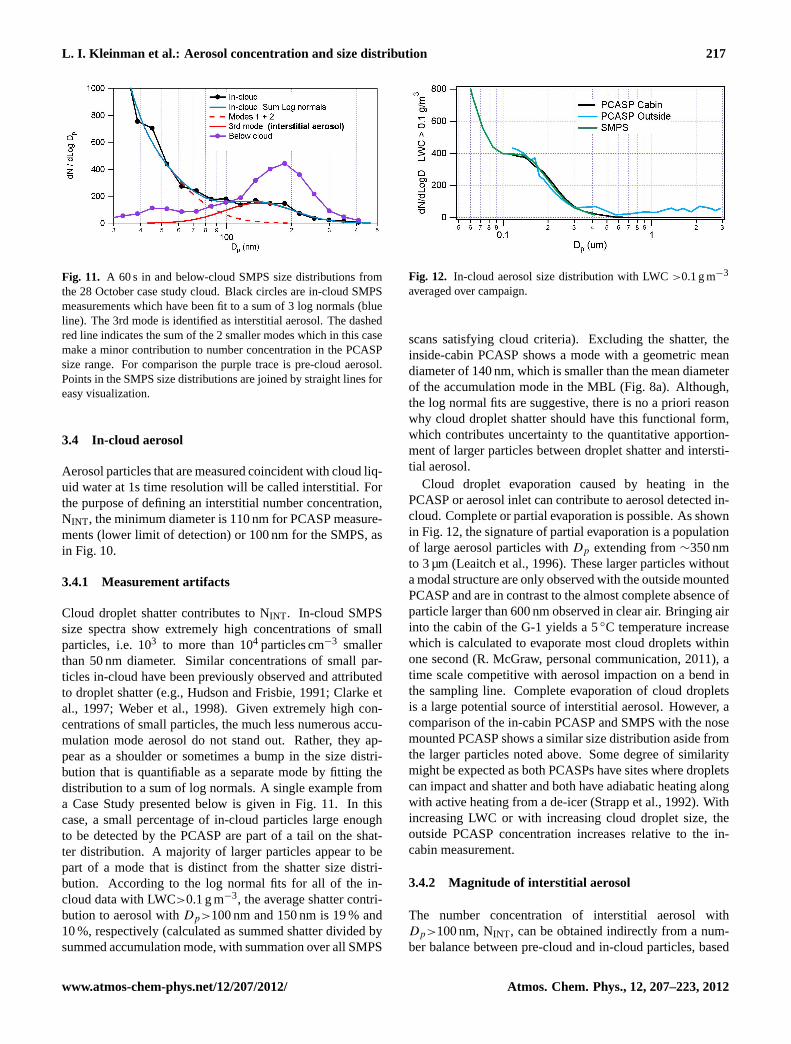
Fig. 11. A 60 s in and below-cloud SMPS size distributions fromthe 28 October case study cloud. Black circles are in-cloud SMPSmeasurements which have been fit to a sum of 3 log normals (blueline). The 3rd mode is identified as interstitial aerosol. The dashedred line indicates the sum of the 2 smaller modes which in this casemake a minor contribution to number concentration in the PCASPsize range. For comparison the purple trace is pre-cloud aerosol.Points in the SMPS size distributions are joined by straight lines foreasy visualization.

3.4 In-cloud aerosol

Aerosol particles that are measured coincident with cloud liq-uid water at 1s time resolution will be called interstitial. Forthe purpose of defining an interstitial number concentration,NINT , the minimum diameter is 110 nm for PCASP measure-ments (lower limit of detection) or 100 nm for the SMPS, asin Fig. 10.

3.4.1 Measurement artifacts

Cloud droplet shatter contributes to NINT . In-cloud SMPSsize spectra show extremely high concentrations of smallparticles, i.e. 103 to more than 104 particles cm−3 smallerthan 50 nm diameter. Similar concentrations of small par-ticles in-cloud have been previously observed and attributedto droplet shatter (e.g., Hudson and Frisbie, 1991; Clarke etal., 1997; Weber et al., 1998). Given extremely high con-centrations of small particles, the much less numerous accu-mulation mode aerosol do not stand out. Rather, they ap-pear as a shoulder or sometimes a bump in the size distri-bution that is quantifiable as a separate mode by fitting thedistribution to a sum of log normals. A single example froma Case Study presented below is given in Fig. 11. In thiscase, a small percentage of in-cloud particles large enoughto be detected by the PCASP are part of a tail on the shat-ter distribution. A majority of larger particles appear to bepart of a mode that is distinct from the shatter size distri-bution. According to the log normal fits for all of the in-cloud data with LWC>0.1 g m−3, the average shatter contri-bution to aerosol withDp>100 nm and 150 nm is 19 % and10 %, respectively (calculated as summed shatter divided bysummed accumulation mode, with summation over all SMPS

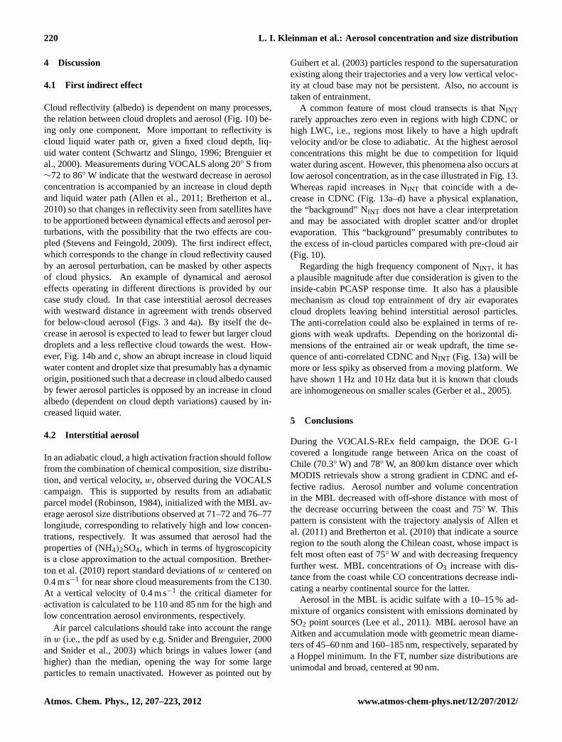
Fig. 12. In-cloud aerosol size distribution with LWC>0.1 g m−3

averaged over campaign.

scans satisfying cloud criteria). Excluding the shatter, theinside-cabin PCASP shows a mode with a geometric meandiameter of 140 nm, which is smaller than the mean diameterof the accumulation mode in the MBL (Fig. 8a). Although,the log normal fits are suggestive, there is no a priori reasonwhy cloud droplet shatter should have this functional form,which contributes uncertainty to the quantitative apportion-ment of larger particles between droplet shatter and intersti-tial aerosol.

Cloud droplet evaporation caused by heating in thePCASP or aerosol inlet can contribute to aerosol detected in-cloud. Complete or partial evaporation is possible. As shownin Fig. 12, the signature of partial evaporation is a populationof large aerosol particles withDp extending from∼350 nmto 3 µm (Leaitch et al., 1996). These larger particles withouta modal structure are only observed with the outside mountedPCASP and are in contrast to the almost complete absence ofparticle larger than 600 nm observed in clear air. Bringing airinto the cabin of the G-1 yields a 5◦C temperature increasewhich is calculated to evaporate most cloud droplets withinone second (R. McGraw, personal communication, 2011), atime scale competitive with aerosol impaction on a bend inthe sampling line. Complete evaporation of cloud dropletsis a large potential source of interstitial aerosol. However, acomparison of the in-cabin PCASP and SMPS with the nosemounted PCASP shows a similar size distribution aside fromthe larger particles noted above. Some degree of similaritymight be expected as both PCASPs have sites where dropletscan impact and shatter and both have adiabatic heating alongwith active heating from a de-icer (Strapp et al., 1992). Withincreasing LWC or with increasing cloud droplet size, theoutside PCASP concentration increases relative to the in-cabin measurement.

3.4.2 Magnitude of interstitial aerosol

The number concentration of interstitial aerosol withDp>100 nm, NINT , can be obtained indirectly from a num-ber balance between pre-cloud and in-cloud particles, based

www.atmos-chem-phys.net/12/207/2012/ Atmos. Chem. Phys., 12, 207–223, 2012

218 L. I. Kleinman et al.: Aerosol concentration and size distribution

Fig. 13. Interstitial aerosol and cloud droplet number in cloud sampled on 28 October (see Fig. 2)(a) Time series of aerosol from inside-cabin PCASP and CDNC at 1 Hz and with 400 s binomial smoothing (red lines). Color bar indicates time in seconds.(b) Scatter plot of 1HzCDNC vs. PCASP NINT . Red line is least squares fit.(c) Scatter plot of high frequency anomaly (1 Hz signal – low frequency component)for CDNC vs. PCASP NINT . Red line is least squares fit.(d) Scatter plot of CDNC vs. PCASP after 10 s box car averaging. Points are colorcoded according to scale in(a) and are joined to indicate continuity. Note that the points fit within the envelope of points in(b) but appearmore spread out because of a change of scale.(e) Scatter plot of CDNC vs. PCASP after 400 s binomial smoothing. Points are color codedas in(a) and(d).

on the assumption that aerosol smaller than 100 nm are notactivated. NINT obtained by number balance is illustrated fora single cloud data point by the blue arrow in Fig. 10. Thefraction of in-cloud particles that are interstitial, defined us-ing average values in the expression (NINT /(NINT + CDNC)),is 0.27. As in Fig. 10, CDNC incorporates a factor of 0.8,based on the assumption that actual CDNC are lower thanreported (see Sect. 3.3). As can be seen from the red linerepresenting a fit to the pre-cloud aerosol, most particles notactivated are at higher aerosol concentration, where compe-tition for water vapor is more likely.

NINT can also be directly measured, again using thecriterion thatDp>100 nm. This is illustrated in Fig. 10for a single cloud data point by a green arrow whichconnects a pre-cloud aerosol concentration with the cor-responding sum of cloud droplets plus measured inter-stitial aerosol. Based on the in-cloud aerosol measure-ments, the total number of in-cloud particles is, on av-erage, a factor of 1.29 greater than the pre-cloud aerosol(i.e. (NINT + CDNC)/NPRE−CLOUD = 1.29). The NINT de-rived by direct measurement is greater than that inferredby particle balance, which by definition gives (NINT +CDNC)/NPRE−CLOUD = 1.0. Allowance for a 19 % contribu-

tion from shatter reduces the imbalance to a factor of 1.20.This factor represents a combination of measurement errorand methodological bias including but not limited to an acti-vation threshold different than 100 nm. The fraction of pre-cloud aerosol not activated (NINT /NPRE−CLOUD) has an aver-age value of 0.48 based on measured values of NINT , whichreduces to 0.39 after accounting for an average shatter frac-tion of 19 %.

3.4.3 Interstitial aerosol – CDNC anti-correlation

Interstitial aerosol were anti-correlated with CDNC in all 102cloud transects. Similar observations have been made by oth-ers (e.g. Gultepe et al., 1996; Wang et al., 2009). As a rep-resentative example we consider a case study cloud observedon Flight 081028a, centered at 75.2◦ W (Fig. 2). Figure 13ashows a 1 Hz time series of CDNC and NINT measured withthe CAS and inside-cabin PCASP, respectively. There aremultiple spikes lasting no more than 1s in which a decreasein CDNC is accompanied by an increase in NINT . There arealso variations on time scales of tens of seconds or longer inwhich the relation between CDNC and NINT is less apparent.

Atmos. Chem. Phys., 12, 207–223, 2012 www.atmos-chem-phys.net/12/207/2012/

L. I. Kleinman et al.: Aerosol concentration and size distribution 219

A plot of CDNC vs. NINT (Fig. 13b) shows an over-all anti-correlation but with considerable scatter. The anti-correlation that is apparent in the high frequency spikes inFig. 13a is partially obscured by changes in pre-cloud aerosoland/or cloud dynamics that are important over spatial scalesof order 5 km and greater. In order to account for the non-uniformity of the cloud, we qualitatively separate low andhigh frequency components. A 400 s binomial filter, sub-jectively selected, has been applied, yielding low frequencycomponents shown by red lines in Fig. 13a. High frequencycomponents called anomalies to avoid confusion with 10 Hzdata presented later on are defined as the difference betweena 1 Hz signal and the corresponding low frequency filteredcomponent. A graph of high frequency anomalies in Fig. 13chas reduced scatter.

Low frequency changes in aerosol and cloud droplets con-tribute to scatter in Fig. 13b. Cloud regions which have dif-ferent aerosol inputs or different dynamics can have CDNCvs. aerosol plots that are shifted relative to each other. InFig. 13d, the original 1s data has been subject to a 10 s run-ning box car average, which is a visual aid to picking outcontiguous points. Lines are drawn between consecutive datapoints and color coded to correspond to the time sequence inFig. 13a. One can pick out 4 or 5 strands that represent con-tiguous cloud portions up to 10 km in length that individuallyshow an anti-correlation between CDNC and NINT . Amongthe 102 clouds transects, this type of structure is common. Ata still larger spatial scale approaching the length of the tran-sect, CDNC and NINT are correlated (Fig. 13e). Dependingon mesoscale structure, the low frequency changes in CDNCand NINT can be correlated, anti-correlated, or scattered.

Higher frequency measurements are useful in interpretingthe presence of interstitial aerosol. Increasing the time re-sponse of cloud droplet measurements to 10 Hz as in Fig. 14,shows that the cloud contains regions in which CDNC de-creases to near zero accompanied by large decreases in LWCbut relatively small changes in volume mean radius. It isexpected that the interstitial aerosol shows similar high fre-quency structure but this is not observable with our samplingline.

A regression between the high frequency anomalies ofCDNC and accumulation mode aerosols has a slope of−2.0for the case study cloud in Fig. 13, approximately equal tothe median slope of−2.1 found for the entire data set of 102clouds. Several factors contribute to the slope being steeperthan minus 1, the value that would be obtained if removalof a single cloud droplet resulted in the appearance of an in-terstitial aerosol particle detected by the PCASP. First is thepossibility of an overestimate in CDNC as suspected from theintercomparison data in Table 2. If actual CDNC are 80 % ofmeasured, correcting the CDNC changes the slope by a factorof 0.8 (i.e. from−2 to −1.6). Second, cloud droplets couldbe formed from aerosol particles smaller than the 110 nmlower limit of detection of the PCASP. Sub-cloud aerosol sizedistributions have a Hoppel minimum at∼75 nm, indicating

Fig. 14. (a)Cloud droplet number concentration,(b) liquid watercontent, and(c) cloud droplet volume mean radius for the samecloud transect and time period used in Fig. 13. Data collected at10 Hz shows increased structure, in particular containing holes withnear zero cloud droplet concentration and LWC. Distance coveredis 35 km, comparable to the size of mesoscale structures apparenton satellite photos. Note change in cloud properties near 11:24:30.

that sometime in the air mass history, particles of that sizewere activated (Cantrell et al., 1999). Third, is a degradedtime response due to mixing in the inlet manifold leading tothe inside-cabin PCASP. This effect has been simulated byconstructing a PCASP signal which is the negative of CDNC,then subjecting it to 3 point binomial smoothing to simulatemixing. The resulting regression slope between the high fre-quency components of CDNC and the synthetic PCASP sig-nal was -1.49, instead of -1 before smoothing. Results de-pend on the degree of smoothing and our choice is meant tobe only illustrative. Supporting evidence for the importanceof time response comes from the PCASP mounted on the air-craft nose which yields a median slope of−1.35.

The case study cloud shown in Figs. 13 and 14 is repre-sentative in many ways, but as a single cloud is not meantto illustrate features resulting from the natural range in adi-abaticity, position relative to cloud top and bottom, aerosolconcentration, LWC, drizzle, and mesoscale structure seenduring VOCALS.

www.atmos-chem-phys.net/12/207/2012/ Atmos. Chem. Phys., 12, 207–223, 2012

220 L. I. Kleinman et al.: Aerosol concentration and size distribution

4 Discussion

4.1 First indirect effect

Cloud reflectivity (albedo) is dependent on many processes,the relation between cloud droplets and aerosol (Fig. 10) be-ing only one component. More important to reflectivity iscloud liquid water path or, given a fixed cloud depth, liq-uid water content (Schwartz and Slingo, 1996; Brenguier etal., 2000). Measurements during VOCALS along 20◦ S from∼72 to 86◦ W indicate that the westward decrease in aerosolconcentration is accompanied by an increase in cloud depthand liquid water path (Allen et al., 2011; Bretherton et al.,2010) so that changes in reflectivity seen from satellites haveto be apportioned between dynamical effects and aerosol per-turbations, with the possibility that the two effects are cou-pled (Stevens and Feingold, 2009). The first indirect effect,which corresponds to the change in cloud reflectivity causedby an aerosol perturbation, can be masked by other aspectsof cloud physics. An example of dynamical and aerosoleffects operating in different directions is provided by ourcase study cloud. In that case interstitial aerosol decreaseswith westward distance in agreement with trends observedfor below-cloud aerosol (Figs. 3 and 4a). By itself the de-crease in aerosol is expected to lead to fewer but larger clouddroplets and a less reflective cloud towards the west. How-ever, Fig. 14b and c, show an abrupt increase in cloud liquidwater content and droplet size that presumably has a dynamicorigin, positioned such that a decrease in cloud albedo causedby fewer aerosol particles is opposed by an increase in cloudalbedo (dependent on cloud depth variations) caused by in-creased liquid water.

4.2 Interstitial aerosol

In an adiabatic cloud, a high activation fraction should followfrom the combination of chemical composition, size distribu-tion, and vertical velocity,w, observed during the VOCALScampaign. This is supported by results from an adiabaticparcel model (Robinson, 1984), initialized with the MBL av-erage aerosol size distributions observed at 71–72 and 76–77longitude, corresponding to relatively high and low concen-trations, respectively. It was assumed that aerosol had theproperties of (NH4)2SO4, which in terms of hygroscopicityis a close approximation to the actual composition. Brether-ton et al. (2010) report standard deviations ofw centered on0.4 m s−1 for near shore cloud measurements from the C130.At a vertical velocity of 0.4 m s−1 the critical diameter foractivation is calculated to be 110 and 85 nm for the high andlow concentration aerosol environments, respectively.

Air parcel calculations should take into account the rangein w (i.e., the pdf as used by e.g. Snider and Brenguier, 2000and Snider et al., 2003) which brings in values lower (andhigher) than the median, opening the way for some largeparticles to remain unactivated. However as pointed out by

Guibert et al. (2003) particles respond to the supersaturationexisting along their trajectories and a very low vertical veloc-ity at cloud base may not be persistent. Also, no account istaken of entrainment.

A common feature of most cloud transects is that NINTrarely approaches zero even in regions with high CDNC orhigh LWC, i.e., regions most likely to have a high updraftvelocity and/or be close to adiabatic. At the highest aerosolconcentrations this might be due to competition for liquidwater during ascent. However, this phenomena also occurs atlow aerosol concentration, as in the case illustrated in Fig. 13.Whereas rapid increases in NINT that coincide with a de-crease in CDNC (Fig. 13a–d) have a physical explanation,the “background” NINT does not have a clear interpretationand may be associated with droplet scatter and/or dropletevaporation. This “background” presumably contributes tothe excess of in-cloud particles compared with pre-cloud air(Fig. 10).

Regarding the high frequency component of NINT , it hasa plausible magnitude after due consideration is given to theinside-cabin PCASP response time. It also has a plausiblemechanism as cloud top entrainment of dry air evaporatescloud droplets leaving behind interstitial aerosol particles.The anti-correlation could also be explained in terms of re-gions with weak updrafts. Depending on the horizontal di-mensions of the entrained air or weak updraft, the time se-quence of anti-correlated CDNC and NINT (Fig. 13a) will bemore or less spiky as observed from a moving platform. Wehave shown 1 Hz and 10 Hz data but it is known that cloudsare inhomogeneous on smaller scales (Gerber et al., 2005).

5 Conclusions

During the VOCALS-REx field campaign, the DOE G-1covered a longitude range between Arica on the coast ofChile (70.3◦ W) and 78◦ W, an 800 km distance over whichMODIS retrievals show a strong gradient in CDNC and ef-fective radius. Aerosol number and volume concentrationin the MBL decreased with off-shore distance with most ofthe decrease occurring between the coast and 75◦ W. Thispattern is consistent with the trajectory analysis of Allen etal. (2011) and Bretherton et al. (2010) that indicate a sourceregion to the south along the Chilean coast, whose impact isfelt most often east of 75◦ W and with decreasing frequencyfurther west. MBL concentrations of O3 increase with dis-tance from the coast while CO concentrations decrease indi-cating a nearby continental source for the latter.

Aerosol in the MBL is acidic sulfate with a 10–15 % ad-mixture of organics consistent with emissions dominated bySO2 point sources (Lee et al., 2011). MBL aerosol have anAitken and accumulation mode with geometric mean diame-ters of 45–60 nm and 160–185 nm, respectively, separated bya Hoppel minimum. In the FT, number size distributions areunimodal and broad, centered at 90 nm.

Atmos. Chem. Phys., 12, 207–223, 2012 www.atmos-chem-phys.net/12/207/2012/

L. I. Kleinman et al.: Aerosol concentration and size distribution 221

In each of three altitude ranges, collectively spanning theFT from 1200 to 3000 m, dew point varied by more than40◦C, showing that within a narrow altitude span, air masseswith very different histories were sampled. The requirementthat an ascending air mass has a relative humidity less than100 %, combined with a strong dependence of temperatureon altitude implies that the lowest dew point air observed(−40◦C) originated above 8 km altitude (assuming a surfacetemperature of 15◦C and a lapse rate of 6.5◦C Km−1, forpurpose of illustration). Conversely, moist air implies a lowaltitude source.

Frequency distributions of CO, O3, aerosol number, andaerosol volume are provided as functions of altitude and dewpoint. Using dew point in place of altitude has the advan-tage of separating air masses according to history and high-lights the different behavior of soluble and insoluble pollu-tants (Kleinman and Daum, 1991). Dew point more clearlypicks up trends in O3 because O3 has a source in the dryupper atmosphere and a MBL sink. There is a pronounceddecrease in aerosol volume with dew point as low dew pointair masses have been subject to cloud processes that haveremoved all but a few percent of their total water. Removedalong with water are soluble substances such as accumulationmode particles that are CCN. The decrease with dew point ofaerosol number concentration is less extreme because of thedominance of smaller less easily activated particles in the FT.The FT population of aerosol, however, does contain someaccumulation mode size particles (Dp>100 nm) which willsubside into the MBL, much the same as O3, thereby provid-ing a source of CCN to replace that lost by drizzle (Clarke etal., 1996, 1997). Relative solubility may play a role in the 5fold increase in the organic aerosol to sulfate ratio with de-creasing dew point. It is also possible that the high ratio atlow Td reflects emission rates in areas not impacted by SO2sources. Even with an elevated organic to sulfate ratio in dryair, the organic aerosol to CO ratio is an order of magnitudelower than observed in day old plumes in the boundary layerin other field studies.

Comparison was made between (a) pre-cloud aerosol andcloud droplets and (b) between pre-cloud air and the sum ofinterstitial aerosol and cloud droplets. According to com-parisons “a” and “b” the fraction of pre-cloud aerosol thatis interstitial is 27 % and 48 %, respectively. In comparison“b” there is a 29 % over-prediction of total particles in-cloud,assuming a 100 nm critical diameter for activation. Dropletshatter and evaporation of cloud droplets during in-cloudaerosol sampling are discussed as possible artifacts. Pursuantto methodological assumptions, droplet shatter contributesclose to 20 % of interstitial aerosol larger than 100 nm, and arapidly decreasing fraction at larger diameter. Adiabatic par-cel model calculations based on measured aerosol composi-tion, concentration, size distribution, and a 0.4 m s−1 verticalvelocity yield a critical diameter for activation between 85and 110 nm, for clean and polluted conditions. While thissupport the use of 100 nm as a lower bound to aerosol diam-

eter in comparisons “a” and “b”, it yields fewer interstitialaerosol than observed.

One hundred and two constant altitude cloud transectswere identified and used to examine relations betweenCDNC and the number concentration of interstitial aerosol(NINT) as measured by a heated PCASP inside the aircraftcabin. In each transect CDNC and NINT are anti-correlated,suggesting that a decrease in cloud droplets by e.g. evapora-tion leads to the appearance of interstitial aerosol. One cloudsampled over a 35 km transect was selected for a case study.Within this cloud there were 4 or 5 regions with distinctlydifferent relations between CDNC and NINT contributing toscatter over the 35 km cloud. Much of the scatter could be re-moved by applying a high pass filter and examining anoma-lies determined as the total signal less the low frequency vari-ation. The in-cloud aerosol concentration contains high fre-quency components that are a possible source of informationon particle activation and/or evaporation sitting on top of alow frequency background, the later partly due to scatter andpartly of unknown origin, that we tentatively associate withan over prediction of interstitial aerosol.

Acknowledgements.We thank chief pilot Bob Hannigan and theflight crew from PNNL for a job well done. Thanks to Robert Mc-Graw of BNL for droplet evaporation calculations. We gratefullyacknowledge the Atmospheric Science Program within the Officeof Biological and Environmental Research of DOE for supportingfield and analysis activities and for providing the G-1 aircraft. Useof a c-ToF-AMS provided by EMSL is appreciated. The VOCALSRegional Experiment owes its success to many people. We wouldlike to single out Robert Wood (Univ. of Washington), ChristopherBretherton (Univ. of Washington), and C.‘Roberto Mechoso(UCLA) for their organizational skills and scientific leadership.S. S. Yum is partially supported by the Korean MeteorologicalAdministration Research and Development Program under GrantRACS 2010-5001. This research was performed under sponsorshipof the US DOE under contracts DE-AC02-98CH10886.

Edited by: C. Twohy

References

Allen, G., Coe, H., Clarke, A., Bretherton, C., Wood, R., Abel, S. J.,Barrett, P., Brown, P., George, R., Freitag, S., McNaughton, C.,Howell, S., Shank, L., Kapustin, V., Brekhovskikh, V., Klein-man, L., Lee, Y.-N., Springston, S., Toniazzo, T., Krejci, R.,Fochessato, J., Shaw, G., Krecl, P., Brooks, B., McMeeking, G.,Bower, K. N., Williams, P. I., Crosier, J., Crawford, I., Connolly,P., Allan, J. D., Covert, D., Bandy, A. R., Russell, L. M., Trem-bath, J., Bart, M., McQuaid, J. B., Wang, J., and Chand, D.:Southeast Pacific atmospheric composition and variability sam-pled along 20◦ S during VOCALS-REx, Atmos. Chem. Phys.,11, 5237–5262,doi:10.5194/acp-11-5237-2011, 2011.

Ayers, G. P., Penkett, S. A., Gillett, R. W., Bandy, B., Galbally, I.E., Meyer, C. P., Elsworth, C. M., Bentley, S. T., and Forgan, B.

www.atmos-chem-phys.net/12/207/2012/ Atmos. Chem. Phys., 12, 207–223, 2012

222 L. I. Kleinman et al.: Aerosol concentration and size distribution

W.: Evidence for photochemical control of ozone concentrationsin unpolluted marine air, Nature, 360, 446–449, 1992.

Brechtel, F. J.: Description and assessment of a new aerosol inletfor the DOE G-1 research aircraft, final technical report of workperformed by BMI under contract #0000058843 to BrookhavenNational Laboratory, August 2003.

Brenguier, J.-L., Pawlowska, H., Schuller, L., Preusker, R., Fisher,J., and Fouquart, Y.: Radiative properties of boundary layerclouds: Droplet effective radius versus number concentration, J.Atmos. Sci., 57, 803–821, 2000.

Bretherton, C. S., Wood, R., George, R. C., Leon, D., Allen, G.,and Zheng, X.: Southeast Pacific stratocumulus clouds, pre-cipitation and boundary layer structure sampled along 20◦ Sduring VOCALS-Rex, Atmos. Chem. Phys., 10, 10639–10654,doi:10.5194/acp-10-10639-2010, 2010.

Cantrell, W., Shaw, G., and Benner, R.: Cloud properties inferredfrom bimodal aerosol number distribution, J. Geophys. Res., 104,27615–27624, 1999.

Chand, D., Hegg, D. A., Wood, R., Shaw, G. E., Wallace, D.,and Covert, D. S.: Source attribution of climatically importantaerosol properties measured at Paposo (Chile) during VOCALS,Atmos. Chem. Phys., 10, 10789–10801,doi:10.5194/acp-10-10789-2010, 2010.

Clarke, A. D., Li, Z., and Litchy, M.: Aerosol dynamics in the equa-torial Pacific Marine boundary layer: Microphysics, diurnal cy-cles and entrainment, Geophys. Res. Lett., 23, 773–736, 1996.

Clarke, A. D., Uehara, T., and Porter, J. N.: Atmospheric nucleiand related aerosol fields over the Atlantic: Clean subsiding airand continental pollution during ASTEX, J. Geophys. Res., 102,25281–25292, 1997.

Clegg, S. L., Brimblecombe, P., and Wexler, A. S.: A thermody-namic model of the system H+-NH+

4 -SO2−

4 -NO−

3 -H2O at tropo-spheric temperatures, J. Phys. Chem. A, 102, 2137–2154, 1998.

Clegg, S. L. and Wexler, A. S.: Densities and apparent molar vol-umes of atmospherically important electrolyte solutions. 2. Thesystem H+-HSO−

4 -SO2−

4 -H2O from 0-3 mol kg−1 as a func-

tion of temperature and H+-NH+

4 -HSO−

4 -SO2−

4 -H2O from 0-

6 mol kg−1 at 25 ˚ C using a Pitzer ion interaction model, andNH4HSO4-H2O and (NH4)3H(SO4)2-H2O over the entire con-centration range. J. Phys. Chem. A 115, 3461–3474, 2011.

Collins, D. R., Flagan, R. C., and Seinfeld, J. H., Improved in-version of scanning DMA data, Aerosol Sci. Technol., 36, 1–9,2002.

Draxler, R. R. and Rolph, G. D.: HYSPLIT (HYbrid Single-Particle Lagrangian Integrated Trajectory) Model access viaNOAA ARL READY Website available at:http://ready.arl.noaa.gov/HYSPLIT.php, last access: January 2011, NOAA Air Re-sources Laboratory, Silver Spring, MD, USA, 2010.

Faloona, I., Lenschow, D. H., Campos, T., Stevens, B., van Zanten,M., Blomquist, B., Thornton, D., Bandy, A., and Gerber, H.: Ob-servations of entrainment in Eastern Pacific marine stratocumu-lus using three conserved scalers, J. Atmos. Sci., 62, 3268–3285,2005.

Fountoukis, C., Nenes, A., Meskhidze, N., Bahreini, R., Conant, W.C., Jonsson, H., Murphy, S., Sorooshian, A., Varutbangkul, V.,Brechtel, F., Flagan, R. C., and Seinfeld, J. H.: Aerosol-clouddrop concentration closure for clouds sampled during the In-tercontinental Consortium for Atmospheric Research on Trans-port and Transformation 2004 campaign, J. Geophys. Res., 112,

D10S30,doi:10.1029/2006JD007272, 2007.Gerber, H., Arends, B. G., and Ackerman, A. S.: A new micro-

physics sensor for aircraft use, Atmos, Res., 31, 235–252, 1994.Gerber, H., Frick, G., Malinowski, S. P., Brenguier, J.-L., and Bur-

net, F.: Holes and entrainment in stratocumulus, J. Atmos. Sci.,62, 443–459, 2005.

Gillani, N. V., Schwartz, S. E., Leaitch, W. R., Strapp, J. W., andIsaac, G. A.: Field observations in continental stratiform clouds:Partitioning of cloud particles between droplets and unactivatedinterstitial aerosols, J. Geophys. Res., 100, 18687–18706, 1995.

Guibert, S., Snider, J. R., and Brenguier, J.-L.: Aerosol acti-vation in marine stratocumulus clouds: 1. Measurement val-idation for a closure study, J. Geophys. Res., 108, 8628,doi:10.1029/2002JD002678, 2003.

Gultepe, I., Isaac, G. A., Leaitch, W. R., and Banic, C. M.: Pa-rameterizations of marine stratus microphysics based on in situobservations: Implications for GCMs, J. Climate., 9, 345–357,1996.

Hallar, A. G., Strawa, A. W., Schmid, B., Andrews, E., Ogren,J., Sheridan, P., Ferrare, R., Covert, D., Elleman, R., Jonsson,H., Bokarius, K., and Luu, A.: Atmospheric Radiation Mea-surements Aerosol Intensive Operating Period: Comparison ofaerosol scattering during coordinated flights, J. Geophys. Res.,111, D05S09,doi:10.1029/2005JD006250, 2006.

Hallberg, A., Noone, K. J., Ogren, J. A., Svenningsson, I. B., Floss-mann, A., Wiedensohler, A., Hansson, H.-C., Heintzenberg, J.,Anderson, T. L., Arends, B. G., and Maser, R., Phase partition-ing of aerosol particles in clouds at Kleiner Feldberg, J. Atmos.Chem., 19, 107–127, 1994.

Henning, S., Weingartner, E., Schmidt, S., Wendisch, M., Gaggeler,H. W., and Baltensperger, U., Size-dependent aerosol activationat the high-alpine site Jungfraujoch (3580 m asl), Tellus, 54B,82–95, 2002.

Hoppel, W. A., Frick, G. M., and Larson, R. E.: Effects of non-precipitating clouds on the aerosol size distribution in the marineboundary layer, Geophys. Res. Lett., 13, 125–128, 1986.

Hudson, J. G. and Frisbie, P. R.: Cloud condensation nuclei nearmarine stratus, J. Geophys. Res., 96, 20795–20808, 1991.

Kleinman, L. I. and Daum, P. H.: Vertical distribution of aerosolparticles, water vapor, and insoluble trace gases in convectivelymixed air, J. Geophys. Res., 96, 991–1005, 1991.

Kleinman, L. I., Daum, P. H., Lee, Y.-N., Senum, G. I., Springston,S. R.,Wang, J., Berkowitz, C., Hubbe, J., Zaveri, R. A., Brechtel,F. J., Jayne, J., Onasch, T. B., and Worsnop, D.: Aircraft obser-vations of aerosol composition and ageing in New England andMid-Atlantic States during the summer 2002 New England AirQuality Study field campaign, J. Geophys. Res., 112, D09310,doi:10.1029/2006JD007786, 2007.

Kleinman, L. I., Springston, S. R., Daum, P. H., Lee, Y.-N., Nun-nermacker, L. J., Senum, G. I., Wang, J., Weinstein-Lloyd, J.,Alexander, M. L., Hubbe, J., Ortega, J., Canagaratna, M. R.,and Jayne, J.: The time evolution of aerosol composition overthe Mexico City plateau, Atmos. Chem. Phys., 8, 1559–1575,doi:10.5194/acp-8-1559-2008, 2008.

Kleinman, L. I. et al.: Interactive comment on “Aerosol concen-tration and size distribution below, in, and above cloud from theDOE G-1 during VOCALS-REx”, Atmos. Chem. Phys. Discuss.,11, C6380–C6384,doi:10.5194/acpd-11-C6380-2011, 2011.

Kley, D., Crutzen, P. J., Smit, H. G. J., Vomel, H., Oltmans, S.

Atmos. Chem. Phys., 12, 207–223, 2012 www.atmos-chem-phys.net/12/207/2012/

L. I. Kleinman et al.: Aerosol concentration and size distribution 223

J., Grassl, H., and Ramamathan, V.: Observations of near-zeroozone concentrations over the convective Pacific: Effects on airchemistry, Science, 274, 230–233, 2006.

Lance, S., Brock, C. A., Rogers, D., and Gordon, J. A.: Waterdroplet calibration of the Cloud Droplet Probe (CDP) and in-flight performance in liquid, ice, and mixed-phase clouds duringARPAC, Atmos. Meas. Tech., 3, 1683–1706,doi:10.5194/amt-3-1683-2010, 2010.

Lance, S.: Interactive comment on “Aerosol concentration and sizedistribution measured below, in, and above cloud from the DOEG-1 during VOCALS-REx” by L. I. Kleinman et al., Atmos.Chem. Phys. Discuss., 11, C5622–C5623,doi:10.5194/acpd-11-C5622-2011, 2011.

Leaitch, W. R., Strapp, J., and Isaac, G. A.: Cloud droplet nucle-ation and cloud scavenging of aerosol sulphate in polluted atmo-spheres, Tellus, 38B, 328–344, 1986.

Leaitch, W. R., Banic, C. M., Isaac, G. A., Couture, M. D., Liu,P. S. K., Gultepe, I., Li, S.-M., Kleinman, L. I., Daum, P. H.,and MacPherson, J. I.: Physical and chemical observations inmarine stratus during the 1993 North Atlantic Regional Experi-ment: Factors controlling cloud droplet number concentrations,J. Geophys. Res., 101, 29123–29135, 1996.

Lee, Y.-N., Springston, S., Jayne, J., Wang, J., Senum, G., Hubbe,J., Alexander, L., Brioude, J., Spak, S., Mena-Carrasco, M.,Kleinman, L., and Daum, P.: Aerosol composition, chemistry,and source characterization during the 2008 VOCALS Experi-ment, Atmos. Chem. Phys. Discuss., in preparation, 2011.

Martinsson, B. G., Frank, G., Cederfelt, S.-I., Swietlicki, E., Berg,O. H., Zhou, J., Bower, K. N., Bradbury, C., Birmili, W., Strat-mann, F., Wendisch, M., Wiedensohler, A., and Yuskiewicz, B.A.: Droplet nucleation and growth in orographic clouds in rela-tion to the aerosol population, Atmos. Res., 50, 289–315, 1999.

McGraw, R., and Liu, Y.: Brownian drift-diffusion model for evo-lution of droplet size distributions in turbulent clouds, Geophys.Res. Lett., 33, L03802,doi:10.1029/2005GL023545, 2006.

Mertes, S., Lehmann, K., Nowak, A., Massling, A., and Wieden-sohler, A.: Link between aerosol hygroscopic growth and dropletactivation observed for hill-capped clouds at connected flow con-ditions during FEBUKO, Atmos. Environ., 39, 4247–4256, 2005.

Parrish, D. D., Trainer, M., Holloway, J. S., Yee, J. E., Warshawsky,M. S., Fehsenfeld, F. C., Forbes, G. L., and Mody, J. L.: Rela-tionship between ozone and carbon monoxide at surface sites inthe North Atlantic region, J. Geophys. Res., 103, 13357–13376,1998.

Rahn, D. A., and Garreaud, R.: Marine boundary layer over the sub-tropical southeast Pacific during VOCALS-REx – Part 1: Meanstructure and diurnal cycle, Atmos. Chem. Phys., 10, 4491–4506,doi:10.5194/acp-10-4491-2010, 2010.

Ramanathan, V., Crutzen, P. J., Kiehl, J. T., and Rosenfeld, D.:Aerosols, climate, and the hydrological cycle, Science, 294,2119–2124, 2001.

Robinson, N. F.: The efficient numerical calculation of condensa-tional cloud droplet growth, J. Atmos. Sci., 41, 698–700, 1984.

Schwartz, S. E. and Slingo, A.: Enhanced shortwave cloud radiativeforcing due to anthropogenic aerosols, in Clouds, Chemistry andClimate – Proceedings of NATO Advanced Research Workshop,Ringberg, Germany, 21–25 March 1994, edited by: Crutzen, P.and Ramanathan, V., Springer, Heidelberg, Germany, 191–236,1996.

Snider, J. R. and Brenguier, J.-L.: Cloud condensation nuclei andcloud droplet measurements during ACE-2, Tellus, 52B, 828–842, 2000.

Snider, J. R. and Petters, M. D., Optical particle counter mea-surement of marine aerosol hygroscopic growth, Atmos. Chem.Phys., 8, 1949–1962,doi:10.5194/acp-8-1949-2008, 2008.

Snider, J. R., Guibert, S., Brenguier, J.-L., and Putard, J.-P.:Aerosol activation in marine stratocumulus clouds: 2. Kohlerand parcel theory closure studies, J. Geophys. Res., 108, 8629,doi:10.1029/2002JD002692, 2003.

Stevens, B. and Feingold, G.: Untangling aerosol effects on cloudsand precipitation in a buffered system, Nature, 461, 607–613,2009.

Strapp, J. W., Leaitch, W. R., and Liu, P. S. K.: Hydrated and driedaerosol-size distribution measurements fro the Particle Mea-suring Systems FSSP-300 Probe and the deiced PCASP-100XProbe, J. Atmos. Oceanic Technol., 9, 548–555, 1992.

Springston, S. R., Kleinman, L. I., Nunnermacker, L. J., Brechtel,F., Lee, Y.-N., and Wang, J.: Chemical evolution of an isolatedpower plant plume during the TexAQs 2000 study, Atmos. Envi-ron., 39, 3431–3443, 2005.

Twohy, C. H., Petters, M. D., Snider, J. R., Stevens, B., Tahnk, W.,Wetzel, M., Russell, L., and Burnet, F.: Evaluation of the aerosolindirect effect in marine stratocumulus clouds: Droplet number,size, liquid water path, and radiative impact, J. Geophys. Res.,110, D08203,doi:10.1029/2004JD005116, 2005.

Wang, J., Daum, P. H., Yum, S. S., Liu, Y., Senum, G. I.,Lu, M.-L., Seinfeld, J. H., and Jonsson, H.: Observations ofmarine stratocumulus microphysics and implications for pro-cesses controlling droplet spectra: Results from the Marine Stra-tus/Stratocumulus Experiment, J. Geophys. Res., 114, D18210,doi:10.1029/2008JD011035, 2009.

Weber, R. J., Clarke, A. D., Litchy, M., Li, J., Kok, G., Schillawski,R. D., and McMurry, P. H.: Spurious aerosol measurements whensampling from aircraft in the vicinity of clouds, J. Geophys. Res.,103, 28337–28346, 1998.

Wood, R., Bretherton, C., Huebert, B., Mechoso, C. R.,and Weller, R., VOCALS-SouthEast Pacific Regional Ex-periment (REx) Scientific Program Overview, available on-line at: http://www.eol.ucar.edu/projects/vocals/documentation/vocalsoverview.pdflast access: January 2011, June 2007.

Wood, R., Mechoso, C. R., Bretherton, C. S., Weller, R. A.,Huebert, B., Straneo, F., Albrecht, B. A., Coe, H., Allen, G.,Vaughan, G., Daum, P., Fairall, C., Chand, D., Gallardo Klen-ner, L., Garreaud, R., Grados, C., Covert, D. S., Bates, T. S.,Krejci, R., Russell, L. M., de Szoeke, S., Brewer, A., Yuter,S. E., Springston, S. R., Chaigneau, A., Toniazzo, T., Min-nis, P., Palikonda, R., Abel, S. J., Brown, W. O. J., Williams,S., Fochesatto, J., Brioude, J., and Bower, K. N.: The VA-MOS Ocean-Cloud-Atmosphere-Land Study Regional Experi-ment (VOCALS-REx): goals, platforms, and field operations,Atmos. Chem. Phys., 11, 627–654,doi:10.5194/acp-11-627-2011, 2011.

Yang, Q., W. I. Gustafson Jr., Fast, J. D., Wang, H., Easter, R.C., Morrison, H., Lee, Y.-N., Chapman, E. G., Spak, S. N.,and Mena-Carrasco, M. A.: Assessing regional scale predic-tions of aerosols, marine stratocumulus, and their interactionsduring VOCALS-REx using WRF-Chem, Atmos. Chem. Phys.,11, 11951–11975,doi:10.5194/acp-11-11951-2011, 2011.

www.atmos-chem-phys.net/12/207/2012/ Atmos. Chem. Phys., 12, 207–223, 2012