Aerosols in gas transporting systems - pure.unileoben.ac.at · Figure 10: Orkiszewski flowpattern...

Aerosols in gas transporting systems

Master Thesis

by

Stephanie Huber

Submitted to the Department of Mineral Resources and Petroleum

Engineering, University of Leoben, Austria

Affidavit

Herewith I declare in the lieu of oath that this thesis is entirely of my own work

using only literature cited at the end of this volume

Leoben, 01.06.2008 (Stephanie Huber)

Acknowledgements

I would like to thank following people for their support:

Univ.-Prof. Bergrat h.c. Dipl.-lng. Dr. mont. Gerhard Ruthammer

Department of Mineral Resources and Petroleum Engineering

Dr. Markus Oberndorfer

Dipl.-lng. Andreas Trieb

Mag. Clemens Zach

Dr. Klaus Potsch

OMV Exploration and Production GmbH

Dipl.-lng. Gernold Weißenböck

OMV Gas GmbH

Dedication:

To my parents Franz and Monika Huber

Table of Content

1. ABSTRACT................................................................................................................10

2. THEORETICAL BACKGROUND............................................................................. 11

2.1. General information on natural gas...............................................................................................................11

2.2. Introduction to aerosol science........................................................................................................................ 12

2.3. Generation of aerosols......................................................................................................................................172.3.1. Retrograde gas condensation...................................................................................................................... 182.3.2. Effect of flow rate on condensation and evaporation.................................................................................212.3.3. Joule Thomson effects................................................................................................................................ 21

2.4. General transport mechanism of aerosols.....................................................................................................232.4.1. Nucleation....................................................................................................................................................232.4.2. Condensation.............................................................................................................................................. 242.4.3. Coagulation.................................................................................................................................................252.4.4. Convection...................................................................................................................................................282.4.5. Diffusion......................................................................................................................................................292.4.6. Interception and impaction of particles......................................................................................................302.4.7. Thermophoresis...........................................................................................................................................322.4.8. Combination of different mechanisms........................................................................................................33

2.5. Settling of aerosols in tubes and pipes............................................................................................................352.5.1. Ordinary flow regimes in pipes for two phases......................................................................................... 352.5.2. Pressure Losses in pipe flow....................................................................................................................... 412.5.3. Temperature Distribution in a pipeline system.......................................................................................... 422.5.4. Aerosol accumulation................................................................................................................................. 432.5.5. Fluid path at branches................................................................................................................................ 44

2.6. Removal of aerosols...........................................................................................................................................472.6.1. Filter technology......................................................................................................................................... 472.6.2. Methods for limitation of the liquids in natural gas..................................................................................50

2.7. Case study: East Javagas Pipeline.................................................................................................................. 52

3. PRACTICAL APPLICATION.................................................................................... 54

3.1. Problem description..........................................................................................................................................54

3.2. Description of the TAG pipeline system........................................................................................................553.2.1. Transition gas in Austria............................................................................................................................ 553.2.2. Topography of the TAG............................................................................................................................. 563.2.3. System equipment description.................................................................................................................... 573.2.4. Pipeline design TAG.................................................................................................................................. 653.2.5. Regulation of gas composition by the ÖVGW G31................................................................................... 663.2.6. Composition of the sales gas in the TAG system...................................................................................... 67

3.3. Analyses of liquid probes................................................................................................................................. 69

3.4. Measurement of HC dewpoint........................................................................................................................71

3.4.1. Measurement of HC dewpoint in the TAG...............................................................................................713.4.2. Problems with the chilled mirror measurement........................................................................................713.4.3. Other methods for measuring the HC dewpoints......................................................................................72

3.5. Phase diagrams of the gas...............................................................................................................................743.5.1. K-factors and mole fractions correlation...................................................................................................753.5.2. Standard correlations of gas composition..................................................................................................793.5.3. Liquids built due to pressure and temperature variation............................................................................853.5.4. Maximum amount of condensates as aerosols at the branching point Weitendorf..................................86

3.6. Glycol vapour pressure analysis..................................................................................................................... 87

3.7. Analysis of flow regime in the TAG...............................................................................................................91

3.8. Vanishing of liquid............................................................................................................................................96

3.9. Technical Consequences and possible solutions............................................................................................97

4. REFERENCES...........................................................................................................98

5. APPENDIX A............................................................................................................101

List of Figures

Figure 1: Single component p-T diagram............................................................................................................. 18

Figure 2: Multi component p-T diagram................................................................................................................19

Figure 3: Quality lines rich gas composition (Dustmann et al.(36)).......................................................................20

Figure 4: Quality lines lean gas composition with compressor oil (Dustmann et al.(36>)....................................20

Figure 5: Joule Thomson inversion curve............................................................................................................. 22

Figure 6: Collision rate dependent on particle size and turbulence!37)................................................................27

Figure 7: Particle relaxation time dependent on particle diameter!6)................................................................... 31

Figure 8: Flow pattern map after Mandhanei39).....................................................................................................36

Figure 9: Flow patterns after Mandhanei39)...........................................................................................................36

Figure 10: Orkiszewski flowpattern map)4°i..........................................................................................................38

Figure 11: Decision tree for flow pattern )9i...........................................................................................................40

Figure 12: Phase envelope shift!5)......................................................................................................................... 46

Figure 13: Aerosol size distribution after normal separation...............................................................................49

Figure 14: Aerosol size distribution.......................................................................................................................50

Figure 15: East Javagas pipeline )13i......................................................................................................................53

Figure 16: TAG pigging and compressor stations from Baumgarten to Arnoldstein..........................................56

Figure 17: TAG topography from Baumgarten to Arnoldstein.............................................................................57

Figure 18: Radial compressor............................................................................................................................... 59

Figure 19: Compressor station in Baumgarten.....................................................................................................61

Figure 20: Nuovo Pignone PCL 603...................................................................................................................... 62

Figure 21: Glycol regeneration unit........................................................................................................................63

Figure 22: Gas chromatogram liquid sample Arnoldstein....................................................................................70

Figure 23: Gas chromatogram liquid sample Arnoldstein and comparison of HTU-AS 32...............................70

Figure 24: HC condensation with the “HC tail”.....................................................................................................72

Figure 25: Dark spot principle............................................................................................................................... 73

Figure 26: Phase diagram: ideal composition......................................................................................................75

Figure 27: Phase diagram: most likely composition with operating conditions.................................................. 78

Figure 28: Phase diagram: worst case with operating conditions........................................................................79

Figure 29: Phase diagram standard correlation.....................................................................................................80

Figure 30: Sampling method for direct measurement in WeitendorP35)............................................................... 81

Figure 31: Phase diagram expanded measurement with measureddewpoint................................................... 83

Figure 32: Phase diagram 1. correlation............................................................................................................... 84

Figure 33: Phase diagram 2. correlation............................................................................................................... 85

Figure 34: Viscosity of 99.5 % TEG.......................................................................................................................92

Figure 35: Calc, vapour pressure of TEG......................................................................................................... 101

Figure 36: Calc, vapour pressure of TEG 2.........................................................................................................102

Figure 37: Calc, vapour pressure of DEG..........................................................................................................103

List of Tables

TABLE 1: REGULATIONS FOR GAS COMPOSITION AND BEHAVIOUR..................................................................... 17

TABLE 2 FILTER DESIGN....................................................................................................................................................58

TABLE 3 GAS COMPOSITION DUE TO ÖVGW G31.......................................................................................................67

TABLE 4 SALES GAS COMPOSITION............................................................................................................................... 68

TABLE 5 IDEAL GAS COMPOSITION 2............................................................................................................................ 74

TABLE 6 MOST LIKELY GAS COMPOSITION...................................................................................................................77

TABLE7 MEASURED DATA................................................................................................................................................ 81

TABLE 8 MEASURED COMPOSITION............................................................................................................................... 82

TABLE 9 TRIETHYLENE GLYCOL DATA........................................................................................................................... 88

TABLE 10 TEG GLYCOL DATA........................................................................................................................................... 89

TABLE 11 TRIETHYLENE GLYCOLVISCOSITYCONSTANTS....................................................................................... 92

TABLE 12 MAXIMUM AMOUNT OF VAP. TRIETHYLENE GLYCOL IN LITRE PER 1 MILL. M3 GAS...................... 101

TABLE 13 MAXIMUM AMOUNT OF VAP. DIETHYLENE GLYCOL IN LITRE...............................................................103

TABLE 14 MINIMUM AND MAXIMUM DATA FOR THE OFFTAKE POINTS AND COMPRESSOR STATION.........106

Author: Stephanie Huber Page: 9

1. AbstractThe transport of gas from regions beyond Europe has increased in the last years due

to the growing energy demand. Therefore problems concerning the gas transport are

of utmost importance. One problem is the existence of fluids in gas transporting

systems and also at the end customers, although drying units and separators are

installed at the compressor stations and branching points. The objective of this thesis

is to show possible scenarios for the generation of fluids in dry gas, which fulfils

certain quality standards like limitations of dew points. Further investigations are the

conditions for liquid hold up and the transport of fluid in pipelines through these units.

Moreover the flow regime of these fluids is analyzed to verify that these liquids are

really transported as aerosols.

The practical part of this work is done for the Trans Austrian Gas (TAG) system,

which transports dry gas. Key findings are that heavy hydrocarbons above C6+ have

a significant impact on the phase diagram of the gas, although their fraction is in the

range of 0.1% of the total gas composition. For this reason the influence of entrained

sealing oil at gas compressors on the phase diagram is researched. Another fluid,

which can be found in pipelines, is glycol. Its phase behaviour and the possible

formation of aerosols is tested.

Another finding is that the geometry of the pipeline system influences the flow of

liquids dependent on the flow regime. This again has an effect on the overall phase

diagrams of the fluid stream in the single branches and can contribute to the liquid

generation.

A phenomenon that is also discussed is that fluids cannot always be found at the

same places in a pipeline system. Reasons for the vanishing of liquid are presented

and improved solutions for the reduction of possible fluids are given.


2. Theoretical Background

2.1. General information on natural gasNatural gas is produced out of geological formations and consists mainly of methane.

Dependent whether it is associated gas, non associated gas or comes from a

different source, the composition of natural gas changes. The other components are

heavier hydrocarbons, nitrogen, hydrogen, sulphur dioxide and carbon dioxide.

These are the parts of the gas, which should be removed, because otherwise

corrosion and liquid drop out can lead to fatal disasters. The amount of Nitrogen is

normally also decreased, because of its non existing heating value. Therefore the

amount of these additional gases in the main stream is regulated in contracts.

Non associated gas is the natural gas that is produced from pure gas wells and

contains only traces of hydrocarbons heavier than pentane. In contrast to this case,

associated gas is the additional product in oil production and is a so called “rich gas”

that is fully loaded with heavy hydrocarbons. Due to the different qualities of the gas it

has to be processed before it reaches the specifications of most contracts. When the

gas then complies with the specifications, it can be transported by the transmission

pipeline system.

These processes start directly after the wellhead and include not only the removal of

the undesired gases, but also the decrease of the water content and solids if present.

The reduction of the unwanted parts of the gas is not perfect and therefore the gas is

sensitive to pressure and temperature changes during the transport, which can lead

to the generation of liquids. A significant impact on this generation can have the

ambient temperature, which can decrease the gas temperature below the dew

points. Another important issue on this topic is that pressure reduction can also

reduce the temperature due to Joule Thomson effects.

The mentioned events lead to condensation of liquids in gas transmission pipelines,

which can be a significant problem, because these fluids are present in the physical

form of aerosols, which are complicate to filter out. Therefore they can accumulate in

undesired areas and can cause failures of machineries during the transport and at

the customer.

Due to the fact that the worldwide gas consumption is steadily increasing and that the

largest gas reserves are often situated far away from the consumers, the transport of


the gas is of crucial importance. For this reason problems connected with the

transport is an object of high interest for the industry and the research.

2.2. Introduction to aerosol scienceAerosols are a fine mixture of liquid droplets and grains in a gas. They have been

studied through the last century till now. Their importance is not negligible because of

their use in pharmaceuticals, chemicals and many other industries. In the last years

the focus in aerosol science was the meteorology, because of the crucial role of

aerosols in global warming.

Generally speaking it has to be said that aerosols are a dynamic constantly changing

system of small particles in a carrier gas. Their behaviour is dependent on the gas,

on the kind of particle and on the particle size distribution.

A very common classification of aerosols according to Parker C. Reist(1) is the division

by physical properties into:

1. dust: consists of solids generated by crushing, grinding, blasting; the size

ranges from sub microscopic to visible; they are small copies from a parent

material

2. fume: solid particles made by combustion, sublimation or distillation; small

sized only up to one pm

3. smoke: an aerosol normally produced via a burning process, where the

combustion process is incomplete; the size of the particles is in the same

region like fumes

4. mist and fog: liquid aerosols, which are produced by evaporation of liquid or

condensation of vapour; the size is normally in between sub microscopic to

20 pm, but can coagulate to 100 pm; therefore they can glide on air currents

5. bio aerosol: an aerosol consisting of living organisms like bacteria or viruses

This first subdivision is often not helpful to characterize the physical properties of an

aerosol adequate enough. Therefore further parameters have to be defined.

Particle size is one of the most important factors to classify aerosols. The

measurement of this is often quite difficult, because of the non spherical shape of


most solid aerosols. Generally only liquid particles form real spheres. Therefore an

equivalent diameter for solids has to be defined. There exist three common types.

The first is Martin’s diameter, which divides the particle into two equal parts. It

depends on the orientation of the particle. Thus the average of some measurements,

which are made in parallel, must be taken. The second is Feret’s diameter, where the

maximum diameter from edge to edge is measured. And the last one is the projected

area diameter, where the diameter of a circle, which has the same area as the

particle, is taken.

For some application these definitions of diameters are anyways not sufficient and

another parameter was introduced for clarification: The particle settling velocity. It

means all particles with the same settling velocity are called equal sized, independent

on their real shape.

Thus it is clear that it is of utmost importance to declare what kind of diameter is

meant, because for every definition another value will be the result. However, not

only the size of a single particle is of interest, but also the distribution of the sizes in

an aerosol, because aerosols are seldom found with only one particle size. These

are then called monodisperse. Normally aerosols contain lot of different dimensions

and are therefore polydisperse. The experience^ shows that under normal

circumstances the log normal distribution fits best for the range of sizes occurring in

the aerosol. This distribution is then described by the mean value and standard

deviation.

As mentioned before aerosols are particles distributed in a gas. To describe now the

behaviour of it, not only the particles are of importance, but also the behaviour of the

gas. This fluid can be characterized by microscopic means as particles sized

comparable to molecules. So the gas consists of small spheres which are moving

randomly through the space. Therefore the statistical mechanics and the kinetic

theory can be applied. A very important parameter is the mean free path of the gas

molecules, which is the average distance a molecule can travel before it collides with

another. The formula is derived by the virtual volume a molecule would sweep out if it

would travel, the number of molecules (n) and the Maxwellian distribution of particles.


1(1)

2 *n * x*o-2

o... collision diameter [nm]

n...number of molecules []

X...mean free path [nm]

To keep now the system of a gas molecule at steady state, forces act on it. The

transfer of momentum, energy and mass are the most important parameters and

they are represented by the viscosity, heat conductivity and the diffusion of a gas.

The other way to visualize the carrier gas would be the macroscopic way. Then the

fluid or aerodynamics is of interest. The flow of the fluid can be generally subdivided

into laminar in the vicinity of the pipe wall and turbulent areas in the middle of the flow

stream. This flow regime is important to know, because most equations are only valid

for one of these parts. The laminar flow regime can be detected in the near pipe wall

region, while the fully turbulent part is in the middle of the pipe. If the medium is

regarded to be incompressible and the gravitational forces are neglected, the only

forces which remain acting on the fluid are the viscous forces and the inertia forces.

The ratio of them is described by Reynolds.

inertia _ forces = Pm d = Pm * v * d = Re (2)

viscous _ forces * v aß d2

pm...density of the fluid [kg/m3]

v... mean fluid velocity [m/s]

d...diameter [m]

p...dynamic viscosity [Pas]

For low Reynolds numbers the flow would be called laminar, viscous or Stokes’s flow.

In this region the viscous forces dominate and streamlines are derived. For fluids

flowing in a pipe the upper limit of the Reynolds number would be around 2100.

Above this the flow is intermediate, where both forces play a significant rule. This is


valid for numbers up to 4000, while above the inertia forces are dominant. Then the

flow is called turbulent and much mixing occurs in the flow.

Another significant factor for aerosol movement in a medium would be the resistance

of the fluid to this motion. An often used parameter to describe this is the drag

coefficient, which relates the drag force with the velocity of the body. Therefore the

drag coefficient is directly dependent on the Reynolds number and for high values it

becomes constant.

FD...drag force [N]

CD... drag coefficient []

v...velocity of the object relative to the fluid [m/s]

Cn =— for laminar flow Cn = 0.44 for turb. flowD Re

For the intermediate region many empirical formulas were derived.

In the laminar region now the resisting force changes because here forces, which act

on the entire body, have to be taken into account. The first, who derived such an

equation for the resisting force of the fluid, was Stokes.

FD = 31:r:zr v * d (4)

d...diameter of the spherical particle [m]

v...particle velocity [m/s]

The assumptions, which are necessary to make this equation valid, are:

• incompressible medium

• infinite medium


continuous medium

• rigid spherical particles

• viscous medium

At the first sight all these assumptions look very far from reality, but for some

applications they are useful. The problem is that for flow in pipes at high pressures

this equation will not be valid. Therefore additional turbulent terms are added.


2.3. Generation of aerosolsThe production of gas can be out of a pure gas field or it can be delivered as

associated gas of an oil field. In general the second type of gas is enriched with

heavier hydrocarbons. Both gases must be treated after production to get rid of water

and higher hydrocarbon components. The gas composition has to meet the

requirements specified in Tab. 1 to be transported via pipelines

Regulations for gas composition and behaviourunit EASEE-gas DVGW G-260

Water dew point °C, 70 bar -8 Soil temp, at pipe line pressure

Condensate dew point °C, <70 bar -2 Soil temp, at pipe line pressure

max CO2 Mol.-% 2.5 -

H2S and COS mg S/m3 5 4.7

Mercaptan mg S/m3 6 6

Total sulphur content mg S/m3 30 30

Oxygen Mol.-% 0.01 3

relative density

Wobbe index kWh/m3

0.555-0.7

13.76-15.81

0.55-0.75

12.8-15.7Table 1: Regulations for gas composition and behaviour

These rules were made to avoid the generation of condensates, water and hydrates

in the system. The gas is usually transported in international systems with a pressure

between 35 and 80 bar. The pressure in the pipes is decreasing over its length.

Therefore the volume of the gas is increasing and the velocity of the gas rises. Hence

the gas has to be compressed at compressor stations to achieve a high enough

pressure level for the transport.

Although these regulations exist, condensates, glycol and lubrication oil is sometimes

found in the pipeline, which means that there must be generation circumstances in

the line, which allow the formation of these liquids.


2.3.1. Retrograde gas condensation

The phase behaviour of natural gas is quite complex, because it does not consist of

only a single component, but of chain of corresponding alkanes. For this reason the

normal p-T diagrams, which is shown in fig. 1, changes, because the dewpoint and

bubblepoint line shift and do not build a single line.

The fig. 2 shows a multiphase behaviour. Between the dew point and the bubble

point line are the so called quality lines, which show constant liquid to gas ratios.

Their origin is in the critical point. For single component substances this is the point

above it is no longer possible to differ between liquid and gas phase. In the multi

component diagram we can see that there exist mixtures of liquid and gas also above

the critical point. The maximum pressure at which this happens is the cricondenbar

and the maximum temperature is the cricondentherm. Therefore at the right side of

the critical point inside the phase envelopes the retrograde gas condensation takes

place. This means that by decreasing the pressure or increasing the temperature into

the two phase region, liquid falls out of the gas as soon as the dew point line is

crossed. This behaviour is the opposite to the properties of all other gases, which is a

consequence of the non ideal behaviour of heavier hydrocarbons. Their solubility in

methane is due to molecular interactions higher than ideal gas equations would

predict it. For this reason alternative equations are taken


For the forecast of the fluid behaviour several equations were setup in the past. The

simplest form is the ideal gas equation.

p *V = n * R * T (5)

p...pressure [bar]

V...volume [m3]

n... number of moles [mol]

R...gas constant [m3 bar/mol K]

T...temperature [K]

This calculation was improved by Van der Waals by introducing factors for the

intermolecular attraction and repulsion forces and the volume of the molecules.

a. ..attraction parameter

b. ..average molecule volume

Although it makes quite better predictions on the fluid behaviour, it is not satisfying for

practical applications. Thus further developments on this section were made by


Soave, Redlich and Kwong (SRK) or Peng and Robinson (PR), to mention only two

of many. They made the phase behaviour also dependent on the eccentricity of the

molecules, which can be large for heavy hydrocarbons.

Of further importance is the gas composition for determining the quality lines of the

gas. A rich gas with high amounts of the ethane plus fraction has shifted its quality

lines to the right side in comparison with a lean gas, which is only contaminated with

compressor oil, although both gases show the same dew point line. This behaviour

can be seen in fig. 3 and fig. 4.

Figure 4: Quality lines lean gas composition with compressor oil (Dustmann et al.(36))


2.3.2. Effect of flow rate on condensation and evaporation

The movement of a droplet can be an influencing parameter for the evaporation of it,

because during the motion at the front of the drop parts of it are taken with the

surrounding gas stream. According to Parker C. Reist(1) in the lower Reynolds region

is the accelerated evaporation balanced by the decrease of this rate at the back of

the drop. For turbulent flow the situation changes. There the size of the particle is of

utmost importance. Drops, which are larger than 40 pm, can react as if they are

surrounded by vacuum. If the particles are smaller, then the relative movement

between the gas stream and the drops is always in the low Reynolds region, because

then the particles move nearly with the same velocity as the gas. This leads to the

conclusion that the flow rate can be neglected only for small particles, while it

increases the evaporation rate for larger particles, when the flow rate rises.

2.3.3. Joule Thomson effects

The Joule Thomson effect describes the temperature change of a gas in

dependence of a pressure change. In most cases the temperature of the gas

decreases with the reduction of the pressure and vice versa. Only when the initial

conditions are below the inversion curve the temperature increases with pressure

reduction. This inversion curve is dependent on the gas. Only in rare cases standard

conditions are below the inversion curve. This would be the case for Helium.

The temperature change of the gas can be described by the Joule Thomson

coefficient, which is substance dependent.

dTVj -T = l I = *(r *«"!)

dp , C' H=const. P

(7)V

Cp... heat capacity at const. Pressure [J/molK]

a...thermal expansion coefficient [1/K]

H...enthalpy [Joule]

pj.T...Joule Thomson coefficient [°C/bar]

V...volume [m3]

T...temperature [K]


It can be seen that the Joule Thomson coefficient is a function of the pressure and

for ideal gases the coefficient is always zero and therefore no temperature changes

occur. For real gases the coefficient is below the inversion curve positive and

negative above. At one pressure two inversion temperatures exist as it is shown in

the fig. 5.

For natural gas the maximum inversion pressure is between 600-700 bar dependent

on the composition. If the composition of natural gas is simplified to consist only of

methane, then the values of the Joule Thomson coefficient lies for 0-50 °C and a

pressure between 40 and 80 bar between 0.5 °C/bar and 0.28 °C/bar as it is shown

in figure 6. The temperature decrease caused by the Joule Thomson effect

contributes to the generation of aerosols, because then the dew point temperature

can be reached.


2.4. General transport mechanism of aerosolsThe transport of aerosols depends on a large number of parameters, which can be

subdivided into internal and external processes (Sager 2007):

Internal processes: 1) nucleation

2) condensation

3) coagulation

External processes: 1) convection

2) diffusion

3) thermophoresis

2.4.1. Nucleation

Generally nucleation is the development of small particles via change of phase. The

necessary requirement is the saturation ratio of the carrier gas.

Ps

p.. .partial pressure

ps... saturated vapour pressure

It depends on the critical saturation ratio if a nucleus is built, or if only a cluster of

molecules is formed, which has only a short lifetime. For homogenous nuclei growth,

this means that the condensation takes place on the formed clusters of similar

vapour molecules. The critical value for the saturation ratio is defined via the Kelvin’s

equation, which shows the dependency of the necessary diameter of a droplet for

growth to the saturation ratio.

Due to this equation very high so called “super saturations” have to be achieved for

small particle sizes, because only particles with a given size, which are built at


saturations at the right side of the line, will grow, while others will evaporate again.

The number of stabile clusters was defined by Pruppacher and Klett(2). Out of their

lists it can be said that it needs at least 1 drop per cubic centimetre and second to

reach spontaneous condensation. The size these aerosols achieve during this

process is normally not the final one, because the particles will grow further due to

coagulation.

The other case is the heterogeneous nucleation, where small solid particles build the

condensation nuclei. Their size can range from some molecules up to a few microns;

this is dependent on the source. These nuclei improve the condensation process in

that way that smaller super saturation is necessary for stable liquid drops, but only a

part of the existing nuclei are involved in the condensation process. How many

particles are activated depend again on their size. So the largest nuclei are the

mostly used and the smaller ones only start to react when the saturation is

increasing. Generally we can further subdivide the nuclei into insoluble and into

soluble ones. For the case of insoluble nuclei there exist two possibilities, whether it is

wettable or not. If it is wettable the Kelvin equation can be used to predict the

condensation behaviour, while for non-wettability the system reaches high

complexity, because then only spheres are built on the surface of the particle. These

spheres at some point form a coating and then normal condensation starts. The

behaviour of this is dependent on the contact angle of the liquid. For soluble nuclei

the critical saturation can decrease below one, but for the application in gas

transporting systems they are not for interest.

2.4.2. Condensation

The growth and lifetime due to condensation and evaporation is also an important

parameter, which influences the transport of aerosols in the gas stream. One

equation, which describes these processes, is the Maxwell equation. The problem is

that it includes many simplifications, therefore Langmuir improved it. For small

particles further improvements were necessary for good predictions and these were

done by Fuchs. With this equation it is theoretically possible to say how long a drop

will exist after its condensation in relation to the surrounding saturation.

This equation shows that if the saturation of the surrounding area becomes one, then

no further evaporation will take place. However the Kelvin equation tells that this can’t

be the truth. Due to Parker C. Reist(1) small droplets will further evaporate because of


curvature effects and the interfacial tension difference also when the media is already

saturated.

2.4.3. Coagulation

As mentioned earlier the dimension of the particle can change due to coagulation.

This is dependent on the Brownian movement of the particles, on to gravitational

forces or turbulence. All these forces lead to velocity differences between the

particles, which are reasonable for the collisions and coalescence of the particles.

The coagulation leads to larger particle sizes, but can not change the overall mass.

Thus the concentration of particles distributed in the gas must decrease. To predict

resulting size distributions numerical models, which predict the dimensions over time,

have to be used. There are also analytical analyses for this approach, which are

representative for the distributions, but not exact. The principle mechanisms of

agglomeration can be classified into (Ho Chi Ahn(37)):

• Thermal agglomeration: The difference in temperature in a fluid induces a

stochastic movement of the particles, which is called Brownian movement.

When the gradient is high the movement increases and the probability that

the particles collide is growing. Therefore more agglomeration occurs.

• Agglomeration through shear strain: Particles in a stream whether laminar

or turbulent can have different velocities due to this current. This lead to

collisions and coagulation, but it only important for particles above one

micron.

• Turbulent agglomeration: Due to the turbulent behaviour of the carrier gas

the particles are accelerated or decelerated. Thus there are again different

velocities of the particles which lead to collisions of them.

• Electrostatic agglomeration: If an electrical field influences the particles,

their velocities will change due to different possible chargeability. This will

lead to agglomerations.

• Acoustic agglomeration: Acoustic waves can undulate the particles, which

make it possible at amplitude maxima that the particles path intersect and

they collide.


• Agglomeration through other influences: The coagulation of particles can

be also an effect of the gravitation or centrifugal forces. These forces are

changing the velocities of the particles in dependence of their size and hence

lead to collisions and formation of other size distributions.

The particle size distribution, which follows from these mechanisms, can be

described by a formula of Smoluchowski . It describes the change in particle density

over time:

K(v,v!).. .agglomeration frequency function: describes, how much of the particles

collide and stick together afterwards

n(v,t)...density of particles in a definite volume at a given time

The first part of the right side of the equation is the production rate of particles with

the volume of v due to collision of particles with the size of v’ and v-v’. The other one

describes the decrease rate of particles, which are lost due to accumulation of

particles with the size v. Therefore this equation is only analytically solvable, when

K(v,v’) is developed correctly for each particle size, the conglomeration of the

aerosols is irreversible and when the particles have spherical shape. Furthermore

only binary collisions are counted and each collision leads to adherence of the

particles.

To derive the equation for the agglomeration frequency the collision rate (Nij), the

reduction of the strike probability (nij) due to fluid mechanics and the adherence

probability (Hy) are taken into account.

KH = X ' x (9)

These parameters are characteristic for the transporting mechanisms with the fluid

dynamic relations and the physical and chemical interactions of the particles.


The collision rate was firstly described over the whole Stokes particle number area in

the 1996 by Kruis and Küster. They developed an equation, which shows the

changes of it due to variation of particle size and turbulence criteria.

*(r"+ +j)

uren...relative particle velocity due to inertial turbulent effects

ure|2... relative particle velocity due to shear turbulent effects

(10)

Out of this equation the forces, which are acting on the particles, while they are

coagulating. With increasing turbulence the Brownian influence decreases, while

other forces rise. The fig. 6 shows the collision rate dependent on particle size and

turbulence.

Figure a) shows the mechanisms for vf =0.1 m/s and e=5*10'4 m2/s3, while figure b) is

a plot for vf =1 m/s and £=1 m2/s3'

The strike probability for turbulent flows is difficult to measure, thus the evaluations of

different authors are only based on numerical calculations. Another name of this

probability is often also collision efficiency. Pinsky (38) solved this problem with two

lateral distances to find the collision cross section, which is according to them not

formed as a circle. This leaded to a higher probability of collision for turbulent flow

than from laminar one.


To solve the equation for particle density over time several analytical methods were

developed, which make assumption far away from real conditions in gas transporting

systems. Therefore the only possibility to solve it would be a numerical one. It is

highly probable that the coagulation of the aerosol particles in the system do not play

an important role.

2.4.4. Convection

The convection, which is for interest in the flow through pipes, is the enforced, where

the stream is induced through compression of the gas. At the beginning of the flow

through pipes the final flow regime is normally not directly reached, but for the long

distances, which the gas flows in the transition pipelines, a fully developed pipe flow

profile can be expected. This means that in the middle of the pipe a turbulent flow is

generated, while at the sidewalls a boundary layer with laminar flow can be

recognized. The width of this layer can be evaluated (Schmidt 2001(4)) with:

8V = d (11)

Re8

5V ...layer width [m]

d...pipe diameter [m]

Re...Reynolds number []

With increasing Reynolds number and decreasing pipe diameter the thickness of this

layer is reducing. Because of the high amount of gas, which is transported through

the TAG, we have to assume that the flow in the pipe is highly turbulent. This has a

high impact on the particle transportation behaviour and on the friction pressure

losses during the transport. These losses are normally described by several models,

which will be discussed in a later part of this thesis.


2.4.5. DiffusionAccording to Sager 2007(6) small particles like aerosols have impulse exchange with

the surrounding gas and other particles. This leads to a stochastic movement of

aerosol, which is not directed. It is called Brown’s particle movement following the

name of Brown’s molecule motion.

The other possibility, why diffusion can happen, is that there is a difference in the

concentration of a substance. The resulting movement (jP) can be described via

Fick’s first law about material flow density.

jp =-Dp * \, (12)

Dp... diffusion coefficient

cp... concentration

The diffusion coefficient is normally dependent on the Boltzmann constant, the

friction factor and the mean temperature. When the temperature is increasing and

the size of the particles is decreasing, then the diffusion coefficient becomes larger.

The diffusion itself is mostly relevant for laminar flow regimes except turbulent

diffusion is meant.

For this case the turbulence will support the natural diffusion, because the turbulent

core of the pipe current adds supplemental mixing and minimizes the concentration

differences. Therefore the maximum diffusion will be between the laminar boundary

layer and the core. This leads to increased particle movement to the sidewalls and

hence to more particle deposition. This movement is quite complex and there exist

several mathematical solution, which are only useable in small ranges. One complex

calculation, which take into account also gravity and pipe surface roughness is that

from Fan and Ahmadi (1993).

The gravity can influence the system only for particles, which are bigger than 1 pm,

because for smaller particles the force becomes negligible due to the reason that the

ratio of the Brown movement to the gravity becomes very small. An important thing is

the flow direction for this kind of segregation, because in some cases the gravity is

supporting the deposition, while in others it can be neglected.


If only the gravity and the resisting force from the fluid to the particle is taken into

account, an equation for the terminal settling velocity could be found.

Cs * P Z * d2p p

18*^(13)

Cs.. .Cunningham slip correction (for particles at the size of the mean free path)

Pp... density of the particle

g...gravity

dp.. .diameter

q...dynamic viscosity

2.4.6. Interception and impaction of particles

The interception of particles is caused by the movement of a particle in the proximity

of a wall. The settling is due to the fact that particles do have some size and the

critical distance for interception is the half of the particle diameter. Out of this we can

see that it is quite an inefficient method for particle separation.

A more important effect is the impaction of particles. Due to the inertia, aerosols can

not follow changes in velocity or direction of the stream immediately. Therefore they

are moving a short way in the original direction of the flow. A parameter to describe

the effect of inertia analytically is the particle relaxation time, which is the

characteristic period a particle needs to change its velocity to at least 63 % of the

new one, which means it reaches equilibrium conditions (Sager*6’ 2007).

TP =r> * d2* Cp p

18*^particle relaxation time (14)

pp ...particle density

dp...particle diameter

Cs.. .Cunningham slip correction

p ...viscosity


Naturally the phenomenon of inertia is for larger particles more important than for

smaller ones as it can be seen in fig. 7. Out of this time it is possible to determine the

distance, which the aerosol can travel in the meanwhile, which is called the particle

stop distance (Friedländer 1977(7)):

5 =n *d2*C

p p

18*^: v ...molecular mean free path (15)

v.. .fluid velocity

pp ...particle density

dP...particle diameter

Cs...Cunningham slip correction

77 ...viscosity

This is then the path an aerosol can move in the old direction before it changes its

way to the new one. Thus it can be said, this is the distance a particle must be away

from the wall, so it is able to stay in the gas stream.

Eminently important is the impaction of particles in tube arches. Also for this effect

many people developed different models. One simple model is a two dimensional


one from Crane and Evans(32). They said that the separation rate is only dependent

on the bow angle (^) and on the Stokes number (Stk):

18*^* — 2

d...pipe diameter

Therefore it would be satisfactory to know the geometry of the bow and the fluid

parameters, and then it is possible to calculate the separation in a bow. The problem

with this idea is that normally monodisperse particles do not occur in nature. Thus for

every size a different separation rate exists.

2.4.7. Thermophoresis

If the temperature in a pipe is not homogenous, but has a certain distribution, then

this acts as a force on the aerosol particles in the direction of the lower temperature.

This phenomenon is called thermophoresis. There exist two possible explanations for

this effect. Smaller particles, which are already in the sub-micron region, collide more

often with the surrounding gas molecules, when they are hot, because then the

relative movement of the gas molecules is faster. Therefore the particles are pushed

in colder regions. For larger particles exists a second explanation. This means that

due to the temperature gradient gas starts to flow in a microscopically stream over

the single particles and this drifts the particles to the colder side. Most of the models,

which were developed for the separation of aerosols, can only predict correct values

for a laminar flow regime, but a simple form for calculation in the turbulent region is

that from Sager*6’ (2007):


D = 1 -T1wTk 1e

, Pr*^(18)

□...separation rate

Te... entrance temperature of the fluid

Tw... wall temperature

Pr...Prandtl number

r 2

Kth =■

2.294: + 2,2* Kn '■C

(1 + 3.438* Kn)'4

1 + 2* - + 4.4* Kn 2

... thermoph. Coefficient (19)ry

Xg, Xw...thermal conductivity parameters of the gas and the wall

Kn =------...Knudsen numberd

(20)

X... mean free path

d...characteristic length of the flow

This model enables the prediction of deposition due to thermophoresis. The problem

with this calculation is that the aerosols are normally not monodispersed, but have a

broad range of sizes. Therefore the evaluation must be done for the mean value of

the distribution.

2.4.8. Combination of different mechanisms

In a complex situation like in the transport of natural gas, where many factors are

influencing the generation and transmission of aerosols it is clear that not only one of

the above mentioned mechanisms is acting. Instead of that a combination of all is

creating the parameters for sedimentation and transport of liquid plugs in the pipes.

Therefore two different approaches exist, which try to balance several of these

effects. The first is the mathematical one, which do no take the physical realities into


account. Therefore the prediction is often wrong, because some effects are supplying

each other, which leads to higher accumulation rates. The problem with both

approaches is that only few different aspects can be taken into account, if it should

stay analytically soluble.


2.5. Settling of aerosols in tubes and pipes

2.5.1. Ordinary flow regimes in pipes for two phases

The flow in pipes is a highly researched topic for the oil and gas industry. In the last

years many models were developed to predict not only the flow regime in horizontal

and vertical pipes, but also for all deviations in between. In general we can differ

between the empirical models, which are often used due to their simplicity. For these

models normally no simulation is necessary and first assumptions on the pressure

draw down and the flow regime can be made. The other models are the mechanistic

models, which are complicated and difficult to handle. Today’s research is at this

region.

In general the flow in horizontal pipes is normally diverted into stratified, slug and

dispersed flow dependent on the amount of gas and liquid, which is transported in

the pipe. For these flow patterns often maps are developed, which allow the

prediction of the flow. The problem with these maps is that nearly all of them were

calculated on the basis of high liquid amounts in the flow. Therefore the maps are

only extrapolated for the region of dispersed flow and hence not accurate for the

prediction in transmission pipelines, where the gas includes only small amounts of

liquid. Hope et al(8) showed this in their study, because they compared several single

phase models with two phase models for the pressure drop prediction of North Sea

pipeline with a small amount of liquid. They found out that the single phase models

give for this situation the better results.

Generally the flow pattern is dependent on the phase densities, viscosities, velocities,

surface tension and the gas liquid ratio. One of the best known maps is that of

Mandhane, which can be easily read in fig. 8. The several flow regimes, which can be

found in the map are displayed in fig. 9.


Figure 8: Flow pattern map after Mandhanei39!

superficial gas vEuccrry.v^. .ft/sec

ELONGATED BUBBLE

ANNULAR-Ml ST

□ ISPERSED BUBBLE (FROTH)

Figure 9: Flow patterns after Mandhanei39!


Two phase empirical models:

They can be subdivided into three classes with increasing precision:

• No slip, no flow pattern model: These ones are the oldest theories, which

were developed in the fifties and sixties of the 20th century, and they are

normally not in use any longer. These models don’t consider the liquid hold

up in the density and the friction factor.

• No flow pattern model: The different velocities of oil and gas are taken into

consideration to predict the liquid hold up and the friction factor along the

pipe. An important model in this category is the Hagedorn and Brown

correlation.

• Slip and flow pattern are taken into consideration: These types of calculation

are still in use to evaluate the flow regime and pressure losses along

pipelines. The most important representatives are Duns and Ros, Orkiszewski

and Beggs and Brill. Some of the newer models can be only calculated on

the computer.

Duns and Ros correlation: It was developed for the flow of oil and gas in vertical

pipes. Therefore it starts over predicting the pressure losses, when the pipe is

smaller than three inch, when the oil gravity is above 56 or below 13° API, when

water is in the fluid stream and for gas liquid ratios above 5000. Duns and Ros

evolved a map with three different flow regimes with transition zones in between.

This map was based on two dimensionless numbers: The liquid velocity number

and the gas velocity number, which include the superficial gas and liquid velocity,

the surface tension and the density of the liquid. Due to the fact that this

correlation has many restrictions, it is not very common any longer.

Orkiszewski correlation: This model was not a new calculation for the flow regime,

but he said that the existing methods do not predict the flow sufficient for all

occurring sections. Therefore he chose different models for several regions. The

resulting flow pattern map is shown in fig. 10.


Dimensionless gas velocity number

Figure 10: Orkiszewski flow pattern mapi4°]

Method Flow Regime

Griffith bubble

Griffith and Wallis slug (density term)

Orkiszewski slug (friction term)

Duns and Ros transition

Duns and Ros annular mist

His assumptions are also only valid for vertical pipe flow. It can be applied on

small tubings below two inches with oil, gas and water flowing below gas liquid

ratios of 5000.

Beggs and Brill: This scheme was originally developed for the flow in horizontal

pipes, but is applicable to all inclinations. Due to its good results it is often used

as basis for mechanistic models. They also evolved a map with different flow

regimes:

Segregated: stratified, wavy and annular flow [(A|<0.01 and Nf^U) or

(A,<0.01 and NFr<L2)]

Transitional: (X|>0.01 and L2<NFr<L3)


Intermittent: plug and slug flow [(0.01<X|<0,4 and L3<NFr2L1) or (X|>0.4

and l_3<NFr<L4)]

Distributed: bubble and mist flow [(X|<0.4 and N^U) or (X|>0.4 and

NFr>L4)]

With increasing velocity of the fluids the flow pattern is changing from

segregated to distributed, where one phase moves as mist in the other. This is

the flow regime, which is important for the aerosol transport. The formula, which

are written below, are necessary for the evaluation of the characteristic numbers.

L2 = 0.0009252 * A-2'46847 Z3 = 0,1 * 2;1'4516

q,um = Usl + Usg Usl = —

Ap

NFr...Froude number

usi,um,usg...fluid velocities

Lt, L2i L3, ^..characteristic numbers

L, = 316* 2°'302

Z4 = 0,5 * 2;6-738

Asante (2000): This model, which he developed, is especially made for gas

transmission lines, which transport only small amounts of fluids. This gas

normally called dry gas can transport liquids like lubrication oil, glycol and gas

condensates but not more than 10 bbl/MMSCF. Therefore only two flow regimes

are possible: The dispersed flow and the stratified flow. To account for these

regimes the model is divided in two sections to describe the transport of the

fluids. The first is a homogenous approach, which is taken, when the flow is

dispersed and the second is a two phase stratified approach, when the flow

changes to the segregated regime.

The decision, which flow is the correct one in the pipe, is based on the calculated

liquid hold up and then compared to the numbers of the decision tree displayed

in fig. 11.


Figure 11: Decision tree for flow pattern Pl

The homogenous flow means that the liquid is dispersed in the dominant gas

phase. To calculate the liquid hold up in the pipe an older model is used. It is the

Hart and Hammersma correlation of 1987. They defined a formula based on the

liquid Reynolds’s number, on the superficial gas and liquid velocity and on the

densities of the fluids, where £L is the liquid hold up.

SL _ USL * Pl

1 ~Sr(21)

lSG

U + 10,4*Re ^“*1 — \PG.

UsL,UsG---Superficial velocities

ReSL---Reynolds number

pL , pG ...fluid densities

On the basis of this formula the flow regime can be decided and that the

pressure drop along the pipeline can be calculated.

The important aspects of the formula are the velocities, which are dependent on

the amount of gas and liquid and the pipe diameter. Therefore to predict the

correct flow regime in the pipe it is necessary to estimate as accurate as possible

how much liquid is transported with the gas. For this reason a worst, a best and

a most likely scenario are evaluated in the later section of this thesis. The other

important parameters are the densities for the liquid and the gas beside the

viscosity of the fluid, which have to be evaluated.


2.5.2. Pressure Losses in pipe flow

The overall pressure losses in a pipe can be described by the following equation:

^PpE + ^PkE + ^Pf (22)

ApPE...pressure drop due to potential energy change

ApKE-■ ■ pressure drop due to change of the kinetic energy

ApF... pressure drop due to friction

If the momentum and the continuity equation are put together and inserted into the

above mentioned equation, then the calculation below can be used. The problem is

that this has some limitations. The assumptions are:

• steady state flow

• no compressors in the system

• adiabatic behaviour

(23)

p ...density of the fluid

g...gravity constant

Q ...inclination

v...fluid velocity

d...pipe diameter

f...friction factor

The equation 23 gives a prediction of the total pressure losses of a fluid of a pipe

flow. The first term describes the elevation or change in potential energy, the second


pictures the losses due to acceleration or the change of kinetic energy, while the last

one characterizes the pressure losses because of friction.

A rule of thumb is that for vertical flow the first term makes about 70-90% of the

overall pressure drop, the second only 0-10% while the last one contributes from 10

30%. This changes dramatically, when the flow becomes horizontal. Then the first

term is negligible, while the last one contains nearly 100% of all pressure losses in

the pipeline. Therefore it is necessary to keep the velocity as low as possible in

horizontal pipes and determine the friction factor exactly.

An important issue for the prediction of the pressure drop is the correct calculation of

the friction factor. The problem with this determination is that there are two

possibilities of turbulent flow. One is the partially rough flow, which is dependent on

the Reynolds’s number and happens for intermediate flow rates. The other is fully

rough flow, where pipe roughness is the determining parameter for the flow regime.

The models with the most accurate evaluation are the Colebrook White and the AGA

equations. The first is the more conservative one, which predicts pressure drops with

a single equation for the flow regime, while the AGA model is based on two different

equations. Uhl (1965) found out that for gas transmission lines AGA predicted the

pressure draw down best.

Because of the above mentioned limitations of this equation normally half empiric

models like Beggs and Brill are taken. This is a model that assumes homogenous

flow. This means that the gas and the liquid phase are treated as a pseudo single

phase and everything is calculated with mixture parameters. If a stratified flow

approach is taken everything becomes more complicated, because than not only the

mixture friction factor has to be calculated, but there must be an evaluation for the

gas to wall friction and for the interfacial friction factor. An example for this model

would be the correlation of Duns and Ros, but also the above mentioned theory of

Ben Asante can be taken for the prediction. In this case it should be the most ideal

one, because it is developed for low liquid loads.

2.5.3. Temperature Distribution in a pipeline system

The temperature distribution of the natural gas flowing in a system is important for the

prediction of the liquid drop out points. The highest temperature can be found after

the compressors due to the heat, which is produced with the compression of the

natural gas. Afterwards the gas is cooled down by large air coolers before it flows into


the transmission pipe. In the section after the compressor stations there is a rapid

decrease of temperature due to a high temperature gradient between the gas and

the surrounding area.

The friction between the wall and the gas contributes also to the decrease of

temperature. Furthermore the forces, which act between the liquids in the gas and

the gas itself, are changing the temperature of the gas. This means that the drag

between the fluids and gas reduce the temperature and the latent heat due to

condensation and vaporization causes also changes.

Another influencing parameter is the undulation of a hilly terrain. During upwards

movement the gas starts to cool down and in the downwards phase the temperature

increases again. This phenomenon can be explained by the fact that during upwards

movement the gas must act against gravity, while in the downward phase, things turn

round.

2.5.4. Aerosol accumulation

Accumulation in turbulent pipe flow:

According to Sager(6) (2007) the accumulation and segregation of aerosols from a

gas stream depends on several parameters. Although his study was done for small

diameter pipes, it is also applicable for larger diameters, because he found out that

the deposition is independent from the pipe diameter, when the Reynolds number is

the same.

One of his conclusions is that for aerosol accumulation the particles must be

subdivided into submicron and supermicron, which means smaller or larger than 1

pm, because of the different segregation behaviour of these particles. The submicron

particles are easier segregated in large diameter pipes, while it depends on many

influencing factors for supermicron aerosols. One thing, which should be considered,

is, if the pipes are horizontal or vertical. When they are horizontal than small pipe

diameters are ideal for separating aerosols.

When the gas stream is cooled down rapidly, then the deposition velocity increases

rapidly. This is the case when the pressure is decreased at branching stations due to

Joule Thomson effect. A slower cooling down of the gas happens during the

transport after the compressors or when the gas is transported above the ground the

ambient temperature is reducing the flowing temperature of the gas.


Another factor, which influences the deposition of aerosols, is the geometry of the

flowing path of the gas. The larger the diameter of the pipe, the easier the particles

can travel with the fluid stream and the fewer are separated. When the turbulence of

the fluid stream increases, which means that the velocity of the gas goes up, then the

also smaller sized particles, on which the inertia forces don’t act as strong as on

larger ones, are separated in the elbows. Moreover the smaller the radius of the bow

and the more the curvature comes close to 90°, the larger is the mass of particles,

which will be segregated in the elbow. An crucial hint for this separation is, that if a

particle draws nearer to the wall than half of its diameter, then it will be deposited.

One principle force, which also acts on particles, is the gravitation, which supports the

settling of the aerosols at the bottom of the pipe.

The problem for defining how long the particles can be transported in the fluid stream

is that due to condensation the size of the aerosols change.

Accumulation of aerosols at expansion places:

At places where the pressure is decreased rapidly like it is often at branching points,

the transport of aerosols is changed. According to Ahmadi et al.(5) the following facts

have to be taken into consideration:

• particles with Stk>1 follow the gas downstream

• deposition of particles at the expansion place increases with rising Stokes

number

• the majority of the submicron particles is deposited at the expansion point

due to recirculation phenomena

• large particles predominantly are transported further

• lift force and gravity are negligible

2.5.5. Fluid path at branches

Gas liquid mixtures partly undergo a separation at branches and junctions in a

pipeline system. This leads to different compositions before and after such

connections. One stream is liquid rich, while the other becomes “drier”. Baker et al.(5)


made experiments about this division with two T-branches in connection find the

optimum segregation constellation for these junctions. The flow pattern they used

where in the region of stratified wavy flow and annular mist, which is quite the same

as expected in the transmission line, when fluid drops out and has time for some

accumulation, and also slug flow, which can happen downhill. This flow pattern is

crucial for the separation that takes place and also the gas split ratio is critical,

because when more gas flows into the branch the velocity of the gas in the branch

increases and also the frictional pressure goes up. Therefore a pressure drop at the

inlet is generated and this sucks more liquid into the junction.

Furthermore the flow rate is important for the split of the liquid into the branch,

because for lower flow rates the forces of inertia act less on the fluid. Therefore it is

easier for it to slide into the branch and higher liquid in the bypass is the output. For

these low flow rates a so called “Flip-flop” effect (Martinez et al.) must be taken into

account. This means that only a part of the gas, how much this depends on the flow

rate, is sucked into the branch, while the total amount of the liquid flows into the

branch. If the amount of gas that goes into the junction is too small, then the whole

fluid will run into the main path.

For disperse flows the segregation of the fluid and the gas is at a T-junction, where

both arms have the same diameter, equal. This means the more gas is flowing in the

branch the more fluid goes in there. If the diameters are different, than only for

dispersed flow the segregation of the fluid stays proportional to the split of the gas

stream. For all other flow regimes a reduced diameter of the branch means a

decreased liquid stream into the junction. This is due to the fact that the branch is

normally not at the bottom or the pipe, but in the centre mounted. Therefore the liquid

has to move up when it enters the side arm.

When the splitting at the branch is unequal, like it is normally for annular and stratified

flow, then the overall phase diagram also changes. The original phase diagram of the

gas is shifted to the right side for the arm with the higher liquid amount and vice

versa. This behaviour can be seen in fig. 12.

The conclusion is that only by knowing the flow pattern at the tee, it can be said

which path the liquid will approximately go.


Therefore the conclusion has to be that branching arms are only significant for the

system, when the liquid amount is high enough to leave the dispersed flow regime

and builds up a liquid film. Then the combination of more T-junctions becomes

important. This phenomenon is already used for phase separation in a petrochemical

plant in the United Kingdom (Baker et al.(5)). However, for this use not only the

optimum combination, but also the correct geometry is of importance. Thus two on

the opposite sides of pipe mounted tees can produce one stream without any gas

and another with only 10% liquid left and this over a wide spectrum of inlet

conditions. Other possibilities to get rid off the liquid are the downward installation of

a branch with a liquid level control valve or without one, which would act as a

constant liquid reducer.


2.6. Removal of aerosols

2.6.1. Filter technology

The problem of liquids in the natural gas transmission system is well known. The

sources are the drying processes, some corrosion, spray effects on flow restrictions

and also the two phase flow of gas. The size of the particles built very significantly:

condensation aerosols: 0.1 - 5 pm

aerosols produced by flow restrictions: 9 - 200 pm

aerosols from liquid entrainment: 400 - 3000 pm

Although the amounts of liquid are normally in a dry gas transmission system very

low, some separators are usually installed along the pipeline. The use of these

separators is dependent on the size of the droplets, because most are not built for

small aerosols.

The separators rely on different segregation mechanisms and consist of several

parts, which use them. These mechanisms are the gravitational force, when it

overcomes the drag force of the gas stream, the centrifugal force, which can be

higher than the gravitational force, the impaction of particles and the Brownian motion

of the droplets. These forces are sorted due to their dependence on particle size.

Primary separation:

The gas enters a separator and flows directly against a deflector plate or into a

cyclone were the velocity of the free fluid is reduced and it drops down to the bottom

of the separator and can be discharged. This removal is effective for aerosols in the

size of 10-100 pm, if the cyclone is properly designed.


Secondary separation:

This form of separation is down by gravity settling. Therefore straightening vanes are

used to reduce the velocity of the gas and bring it down to laminar flow. Due to this

decrease the free fluid starts to accumulate on the plates and drops down to the

liquid outlet.

This form of separation is only possible for big enough droplets. For smaller sizes the

gravity force becomes negligible and the aerosols don’t accumulate. To get rid of

these particles it is necessary that they agglomerate, before they can be separated.

Mist extraction (demister):

This part of the separator consists of a wire mesh package with small porosity. The

gas flows through this mesh and the liquid droplets coalesce on the wires. When they

are big enough, the droplets start to fall down and are then discharged at the bottom.

The maximum thickness of these packages is normally 150 mm, because beyond

this the total separation rate can’t be increased sophisticated^. A problem for this

part of the separator can be, if the liquid amount is larger than calculated, because

then it gets flooded and parts of the fluid enter again the gas stream. This form of a

separator can segregate droplets of a size from 5-10 pm, but the extraction rate is

not 100 %. The only possibility to separate also smaller particles is a filter separator.

The other possibility to reduce mist is a plate fin. This uses the effect of impaction,

because the gas stream must flow between such plates, while the droplets can’t

follow fast enough and collide with the fins. Due to the velocity change the drops start

to accumulate on these plates.

When gas is only dried with usual separators, then some liquid is normally left in the

gas stream. The size of these particles is according to the scientific report of Pall

corp, the following, showed in fig. 13:


Due to the fact that the gas flows always over some separation units, we can say that

this must be the size distribution of the aerosols in the gas. Naturally there are some

changes during the following flow period because of some condensation of liquids

and the coagulation of particles. But if a filter separator is built directly after a normal

separation unit, then this should be the aerosol distribution, which it should be able to

extract.

Filter separation:

This type of separation is used for very fine solids and aerosol extraction. Aerosols in

gas streams can be produced by condensation or by fluid entrainment in the gas

stream. The particles, which are built through condensation, are normally smaller

than 3 pm, while the second ones are larger. The measurement of aerosol size

distribution can be done with a cascade impactor, but it is rarely made because of the

too small utility in comparison to the price.

The particles, which such a separator can remove, are in the range of 0.1 pm and

therefore in the smallest class of aerosols, which occur in natural gas streams. In the

air also smaller aerosols are possible as it can be seen in the fig. 14.


Figure 14: Aerosol size distribution

2.6.2. Methods for limitation of the liquids in natural gas

The most common way to minimize the amount of liquid in the gas stream is to write

a paragraph about the gas quality in the contract. Often this is done with a sentence,

which was constructed at the AGA Gas Measurement Committee Report 4a in 1971:

“The gas shall be commercially free from dust, gum, gum forming constituents and

liquids at pressure and temperature at which the gas is delivered.” The problem in

this formulation is that with reduction of pressure and temperature liquid can drop out

after the delivery. Then the contractor is not reasonable for the liquid, but it is present

in the gas. Therefore also other regulations are used to get liquid problems under

control.

Some corporations use the determination of a maximum heating value to regulate

the liquid drop outs. However, the heating value of a gas is not necessarily high,

when the C6+ value is high and also the other way round. For example when a gas

contains much ethane and no C6+ fraction the heating value is high, but the

hydrocarbon dewpoint would be low.

Another tool sometimes used is the control of the percentage of C5+ or C6+ in the gas

stream. This specification can also not provide that liquid will drop out, because not

only the amount of C6+ but the composition is reasonable for the hydrocarbon

dewpoint. This composition is changing over the length of a pipeline and thus at

some points in the pipes liquid can condense.

Hence the most reliable possibility to prevent fluid drop out is to limit the hydrocarbon

and water dewpoints themselves. The problems related to this are the inexact

measurement and that always only one dewpoint for a specified pressure can be


measured. Therefore it is possible that liquid is built due to retrograde condensation

or because of a composition change downstream the measured point.

Another way to solve this problem is the reduction of heavy hydrocarbons with low

temperature gas drying units. These facilities cool down the gas stream below the

dewpoint, then the fluids condense and at least they are mechanical removed.

Several kinds of these constructions are known. Generally they can be divided into

low temperature installation with gas expansion, such with a refrigeration unit and

units with expanders.

A method to limit the glycol amount in the gas is to change the dehydration

equipment to adsorption units. There the gas flows through a drying bed, where the

water is removed. These beds must be regenerated, when they are loaded, then they

can be used again. It is possible to remove also heavy hydrocarbons (C6+) with these

installations, but for this kind of cleaning the regeneration cycles must be shorten

drastically from several hours to around 20 minutes.


2.7. Case study: East Javagas Pipeline

The East Javagas pipeline, shown in figure 15, connects the isle Pagerungan with

Java Island. It is around 400 kilometres long and transports dry sales gas. The

maximum capacity is at 600 MMSFD with an inlet pressure of 1800 psi. Actually it

transports at a pressure of 1200 psi half of the designed volume.

During the operations in the Pagerungan plant a failure occurred and the dry gas

composition changed to wet gas. This means that the fraction of the heavy

hydrocarbons increased. Due to this problem liquid condensed in the pipeline. More

than 430 barrels were caught in liquid slug catchers. The question, which came up

afterwards, was whether some fluids were left in the system or not.

The problem was simulated with the computer program OLGA. Therefore the

necessary data was collected and then six different cases were simulated. The

conclusion how the liquid behaved in the pipeline were the following: The fluid, which

condensed in the pipe, started to accumulate 20 hours after their building at the low

points of the pipeline. An additional factor for the accumulation was the slope after a

low point. The higher it was the larger was the liquid accumulation. An experiment

was done with water to get more details about the behaviour of the fluid in the pipe.

This water also accumulated at the bottom points and when no more liquid came

from the upstream part of the pipe, the liquid slug got removed due to the high

velocity of the gas. After seven days the first liquid flowed out of the pipe and after

ten days the whole system was dry again. This experiment showed that in a pipe

were permanent gas flows no accumulations can exist over long periods, when the

gas velocity is high enough.


Figure 15: East Javagas pipeline nsi


3. Practical Application

3.1. Problem descriptionIn the year 2004 the GasNetz Steiermark determined liquids in the pressure

reduction station Bauernfeind in Rothleiten and at their customer Mayr Melnhof in

Frohnleiten. For this reason the high pressure pipeline system, which lies before

these points, was checked and fluids could be determined at the stations G4 and G5.

These liquids were analysed and the results have been that they were a product of

machine oil of HD 32 from OMV and unidentified machine oil, which possibly comes

from other compressor stations not controlled by OMV. The rest of the fluid was a

mixture of aqueous triethylene and diethylene glycol.

No significant amount of these liquids was separated in the upstream high pressure

pipelines of OMV, although filter separators are installed and checked continuously.

These fluids can be found in the downstream region, despite this fact that before

every compressor station and also at the off take points the gas was filtered. The

question is whether the particles are too small to be filtered or are they generated at a

point after the filters.


3.2. Description of the TAG pipeline system

3.2.1. Transition gas in Austria

Today Austria has a key position for the transport of Russian gas to Europe. This is a

consequence of a long tradition, which started already in the 1950's, when people

thought about the necessity of the gas import for Austria. This leaded to the building

of the PVS, the “Primärverteilungssystem”. It started to work in 1968 and had a

length of 351.9 km. However since the 1970's the first real transition pipeline was

operated, the TAG 1. The first gas flowed through it in 1974. This was the time when

Austria as the first country made a contract with the UDSSR. The pipeline system

was enlarged in the next years to bring the gas not only to Italy, but also to Slovenia

and Hungary. The increase of the system, made it necessary to build additional

compressor stations along the lines. Today along the TAG three compressor stations

exist. The largest is located in Baumgarten, Niederösterreich, where now the seventh

compressor starts its work. The others are in Grafendorf, Steiermark and in Rüden,

Kärnten. The gas that flows nowadays through the TAG flows on the one hand from

Russia and on the other hand from the Slovakian gas storage in Lab. It is separated,

filtered and measured in Baumgarten, when it enters the station. There also the

quality of the gas is controlled continuously by a gas chromatograph. Three times a

week the hydrocarbon dewpoint is measured and the water dew point is constantly

controlled. If it comes above minus six degree Celsius, the gas is directed over the

glycol dehydrating units. It is possible that this is not the case during a year, but in

2007 the glycol units worked already for 2 weeks, one in August and the other in

October. During every start up phase some glycol is lost into the system. The amount

of glycol that is lost in this phase can be several hundred litres of glycol. Afterwards

during normal operation the losses are very low and can be nearly neglected.

The amount of gas that flows through the TAG system in one year exceeds 41.5

billion cubic meter of gas and is still increasing. To provide corrosion and failures at

the compressor stations the gas is filtered when it enters a station. However the gas

is already dried and only small amounts of liquid accumulates there. These filters are

designed for one micron diameter particles, so that only very small particles could

migrate through the system and this would normally not harm the compressors.

These compressors are driven by powerful gas turbines with up to 22 MW power.

The entrance pressure of the compressors is at 45 bar and the output pressure


reaches 70 bar. All parts of the TAG pipeline system are piggable and every 5 years

intelligent pigs are driven through the pipes. This provides that no corrosion failures

can happen and that no liquid accumulates in the system.

3.2.2. Topography of the TAG

The TAG pipeline, displayed in fig. 16, starts at the Slovakian border and ends in

Arnoldstein at the Italian border. In between are three intake points at Baumgarten,

where also the first compressor station is located. The other nine offtake points are

marked at the map above. They supply the Austrian gas distribution system and at

Weitendorf the SOL pipeline system starts to Slovenia. To achieve the necessary

pressure in the pipes three compressor stations are located along the line. The first is

in Baumgarten. There are four GE Frame 3 gas turbines with 11 MW and three PGT

25 DLE with 22 MW ISO power, which are compressing the gas up to 70 bar. At this

station the gas gets also dehydrated via five glycol drying units and it is filtered to get

rid of the solid particles which could move with the gas. Moreover the first fiscal

metering station is installed at Baumgarten. The others are at Arnoldstein and the

other offtake points along the pipeline.

The second compressor station is in Grafendorf approximately 135 kilometres behind

Baumgarten and the last is in Rüden 150 kilometres behind Grafendorf.

Another installation in the pipeline are the safety valves every 20 kilometres, which

can isolate the sections of the TAG for maintenance or when a problem with leakage

occurs. These chokes can be operated by the OMV gas dispatching centre in Vienna


or from the local compressor stations. The total amount of valves is 36 distributed

over all three lines.

The topography of the TAG shows an undulating hilly terrain as it can be seen in fig.

17, where the changes between minimum and maximum sea level are very large.

The top point of the pipelines TAG 2 and TAG Loop lies above 1200 meters, while

the lowest point is less than 200 meters, which means a height difference of more

than 1000 meters. The TAG 1 doesn’t make these big jumps and has as maximum

diversity around 400 meters difference between top and bottom.

3.2.3. System equipment description

Filtration technology:

The separation in the TAG is done at every compressor station and also at the

branching stations. For that normal separators based on segregation forces and also

some filter coalescers are used. A new coalescer from “Filtan” was installed in

Weitendorf last year for special protection of the “Gasnetz Steiermark”. This

separator has the following design parameters:


max. gas amount 250 000 Nm3/h

min. working temp. -10 °C

max. working temp. +50 °C

min. working press. 50 bar

max. working press. 70 bar

coalescing area 16 m2

separation rate >1 pm 99.90 %

>3 pm 99.99 %

pressure drop -100 mbarTable2: Filter design

These parameters should be sufficient to filter 80 to 90 percent of all aerosols in the

gas stream, because the aerosol distribution after normal separators is mostly above

1 pm. The amount of fluid in the separator, which was found since the filter was

installed, was in the range of 15 litres. This means that in one year since the

installation a fluid amount of about 1.5 to 3.75 litres flew through the separator into

the pipeline net of the GNS. The average gas amount per hour is 74 073.31 m3

When this value is summed up for one year leads this to an amount of 648 882

195.6 m /a. The mass of 3.75 I in the gas is equivalent to a percentage of 5.8*10'

%.

Gas turbines and compressors:

During the flow of gas from the wellhead to the customer it has to be compressed

several times due to pressure losses. Also when it should be stored in an

underground gas storage and the most important compression is for the international

gas transmission lines. These pipes are usually made for operating pressures

between 50 and 70 bar.

In general there exist two different types of compressors for natural gas compressing.

The reciprocating compressor, which is built for low flow and high pressure ratios and

the dynamic compressor, which is made for intermediate to high flow and lower

ratios. It is subdivided into radial and axial compressors, which are only different in

the compressing process and size. A radial one can be seen in fig. 18.


According to the Standard handbook of petroleum and natural gas engineering the

advantages and disadvantages can be summed up to the following:

Advantages of the dynamic compressor:

• low installation costs

• low maintenance costs

• high equipment dependability

• few service

• big volume capacity

Advantages of the reciprocating compressor:

• flexibility

• high efficiency and few energy supply costs

• high pressure ratios

• small sensitiveness to composition and density changes

A problem, which can occur with the dynamic compressors, is the surge. This means

that the compressor cannot add enough energy to the fluid stream that it can


overcome the internal system resistance. So at a given pressure the volume of gas

goes below a certain limit and the stream breaks down. This leads to an inversion of

the flow. If this is repeated several times, the compressor can be completely

destroyed. Thus normally suction valves are installed behind a compressor. Another

problem can be liquid at the compressor. Already small amounts are sufficient to

generate fatal errors. For this reason drying units are installed at the entrance of a

compressor station.

There are several possibilities to drive a compressor. One is a gas turbine. The

functionality of a gas turbine is based on circle process called the Joule process.

There air is compressed over several steps and the swept into a combustion

chamber, where it is mixed with gas, ignited and then burnt. This generates hot gas

which drives the motor itself and the following compressor. The turbines can be

constructed with one shaft. For these types the motor and the compressor can be

only driven at the same engine speed. The type with two shafts can be divided into a

gas generator and a power turbine part. The gas generator unit has some turbine

parts on it, which drive the compressor, while the power turbine is on the second

shaft mounted with the motor. These units drive then normally a separate

compressor unit, which is used to compress the transition gas.

Other possibilities to drive a compressor unit would be a gas motor, an electric motor,

an otto motor or a diesel engine. The choice of the driving unit depends on the

availability and the operation field of the compressor.

The compressor system itself consists of impellers and stators, which firstly

accelerate the sucked gas and therefore the kinetic energy rises. Then the gas hits

the stator, where this energy is changed into higher pressure and afterwards the next

impeller follows. This compression of the gas leads to high temperatures, therefore

the gas and the compressor needs cooling installations.

A totally other concept of compression has the reciprocating processor. It changes

the circulating movement of the driving unit in an oscillating movement and then via a

piston in compression of the gas. It is possible to build several types of these

machines. They can be adapted as single acting or double acting. Another difference

is if they are dry or lubricated. The first is very expensive, because everything must

be constructed very smooth for this type of compressor, otherwise the wear would be

extremely high. The problem with the second type of compressor is that it pollutes the

compressed gas with oil. This oil can partly go into the gas phase and changes

therefore the overall composition of the gas. Although reciprocating compressors are


not used for the international gas transmission, the gas can come in contact with the

oil at its way from the well head to the transmission line.

In Baumgarten GE NP PGT 25 DLE gas turbines and GE NP 41S3002 RC (Frame 3)

are installed.

Figure 19: Compressor station in Baumgarten

PGT 25 aero derivative Gas Turbine:

The PGT 25 is a two shafted aero derivative gas turbine, which consists of a gas

generator and a power turbine. The gas generator is a LM 2500, which is also used

in aircrafts. It is built up of a 16 stage axial flow compressor, which can achieve a

maximum pressure compression ratio of 18:1. There are inlet guide vanes and

adjustable stator vanes, which are supporting the operating features at the

compressor.

The power engine itself is the PGT 25 with 6500 RPM design speed with two

expansion stages. The blade rows are at nozzles designed on cobalt, while the

blades of the rotor itself are made on nickel base. The gas temperature on the inlet to

the power turbine is quite moderate to enlarge the fatigue failure safety.

After the turbine a compressor type PCL- pipeline centrifugal compressor- is installed.

A typical PGT 25 can be seen in fig. 20.


Figure 20: Nuovo Pignone PCL 603

Dehydration technology:

To reduce the water content of natural gas, which is normally carried out of the

reservoir, several dehydration units have been developed. They can be divided into

drying units with liquid absorption substances and with solid adsorption units. In

Austria normally triethylene glycol is used. In earlier days also diethylene glycol and

monoethylene glycol were often taken. Due to better absorption character of TEG,

the use of other glycols was minimized.

The chemical composition of TEG is C6H14O4:

It is built of ethanol and additional OH groups, which increase the ability of alcohol to

take humidity of a gas and hold it. Therefore it is used to reduce the water dew point

of gas in the range of 25 to 35 degree Celsius. The normal use for dehydration is

downstream of a separator, which sweeps out the larger droplets of water. The gas

comes into contact with the glycol in a contact tower with at least four bubble trays.

The lean glycol becomes dispersed with the gas and absorbs the water. Then the dry

gas runs through a demister where the glycol droplets should be held back and

accumulate. However there exists a consumption of glycol during this process, which

comes on the one hand from the distillation process for the regeneration of the rich

glycol, but on the other hand it is caused by the carry over of some glycol to the


pipelines with the dry gas. Normal consumption rates are between 5 and 16 litres per

million cubic meters of gas.

Problems with TEG might be foam generation, which can occur when condensates

are not totally swept out of the gas at the previous separator. This generation leads to

insufficient rich glycol discharge at the bottom of the tower. For this reason the level

of glycol rises and reaches at a sudden point the gas inlet and is then taken into the

transporting line. To avoid this problem, scrubbers should be installed in the

separator or defoaming agents should be mixed into the TEG. A typical installation

can be seen in fig. 21.

flbsorbei Glycol regeneration

Figure 21: Glycol regeneration unit

Dehydration process:

The normal process is the following for dehydrating the glycol:

The gas comes from the well to the station and enters a first separator to sweep out

the free liquid droplets. Then it enters the contact tower at the lower end, where a

scrubber separates the condensates and water, which are generated during the

upstream movement of the gas, and it is preheated before contacting with the glycol.

The wet gas is moving upwards and comes into contact with the lean glycol, which is


moving down. At the upper end the dry gas is leaving the tower and in a heat

exchanger the temperature of the lean glycol is equalized to the temperature of the

gas. The glycol itself is pumped in a closed cycle. After leaving the absorber at the

lower end as rich glycol, it comes into a heat exchanger, where the glycol is

preheated. The next step is that it enters the distillation column, where the glycol is

dried via fractional distillation. The reboiler below is normally directly fired by a burner,

and heats up the glycol. Therefore the water is evaporating out of it and moves up

through the column directly to the atmosphere. If a part of the glycol is taken with the

water vapour, then it condenses again at some cooling features at the upper part of

the column and drops back. This don’t have an efficiency of hundred percent,

because as mentioned above between 5 and 16 litres per million cubic meter dried

gas is lost. The now again made lean glycol can be concentrated up to 99 percent.

The hot glycol has to be cooled down, because the absorption process is very

sensitive to contact temperature changes. Thus the hot glycol is used to preheat the

rich glycol and then comes into a second heat exchanger where gas and glycol

temperature are equalized.

Dependent on the concentration of the glycol the circulation amount, which is

necessary to dry the gas, is increasing. Normally a rate between 25 and 60 kg TEG

per litre water vapour is chosen. For the reconditioning of the TEG the fractional

distilled. This generally is sufficient since the boiling of water is at 100°C whereas the

boiling point of TEG is at 285.5°C. Hence the reboiler temperature is not above

204°C, because it is sufficient for the reconcentration and TEG starts to decompose

thermally at this temperature, when it is heated further. The thermal cracking from

TEG to DEG can partially happen below this temperature and may be the reason for

finding DEG in the liquid samples. Another possibility to increase the glycol

concentration would be vacuum distillation or the use of stripper gas, which lowers

the partial pressure of water.

Corrosion problems with TEG:

The TEG, which is carried out from the dehydration units to the pipeline system, can

lead to the corrosion of the line. The pH value of the TEG is normally decreased

because of thermic processes. This TEG in the system has longer contact with the

gas as usual. Therefore it enriches with water and accumulates at the deepest points

of the line. Then it acts like an acid and starts destroying the pipe.


To reach very deep dewpoints or if the gas temperature is high glycol is not the

optimal choice. For these cases packed bed with adsorption processes should be

taken.

Under the conditions usually found in transport pipelines, glycols exist in liquid

phase.

The melting point of diethylene glycol is at -7.8 °C and for triethylene glycol at -4.3 °C

at one bar, while the bubble points are at 245.5 and 288.0 °C. Due the reason that

the operating pressure is much higher and the operating temperature is below the

boiling point, it is not expectable that the glycol will change its phase.

3.2.4. Pipeline design TAG

The TAG pipeline system consists of the TAG 1, which was installed in 1974. It has a

pipe diameter of 38” and 36”. It has a length of 382 km and is constructed of carbon

steel X-60. The next pipeline, which was installed, was the TAG 2 in 1988 with a

length of 377 km, the material of X-70 and a diameter of 42”. The last expansion was

made with the TAG Loop 2, which was made in several stages. The last one was

finished in 2006. It has a length of 376 km, a material of L 485 MB and a diameter of

40”.

All three lines are laid in a minimum depth of 1.5 meters except for river crossings.

There exist only underwater solutions and no crossing via bridges or elevators. The

most important rivers are the Danube, where the pipes have to cross a length of 970

meters and the Drau with 468 meters.

The whole system is only constructed for the transport of sweet gas, so the acid

components as CO2 and H2S must not exceed very small limitations. Further

construction boundaries are the operating pressure of 70 bar and the temperature of

50 °C. All pipes are at some point interconnected and share the same pressure level.

The inspection and pigging stations are located at a maximum distance along the

pipe line of 70 kilometres. At these points the pigs for dewatering and inspections can

be put into the line or taken out. Every six years in the TAG 1 and every eight years in

TAG 2 and TAG Loop 2 intelligent pigs are used to control wall thickness and areas

of corrosion problems and cracks.


The first branching station is located in Eggendorf and supports the distributing

system of EVN. It is connected with the node Wiener Neustadt and the EVN pipe line

South West 2. The used pipe for the supply is a 16” one, which is branching here

from the main TAG stream with 38” at this point. The next branch is Grafendorf with 8

inch, where the customers are BEGAS and STGW. One of the liquid samples was

delivered by BEGAS. At St. Margarethen a side arm with 6 inch diameter is installed

for the STGW. The following branch is located in Weitendorf and has a 16 inch pipe

connection. The customer here is the STGW, which reported problems for this line

with liquids. The other arm in Weitendorf is a 20 inch connection with the SOL, where

also some liquid problems were recognized at the Murfeld. The next junction is

placed in Sulmeck-Greith, which is feed via an 8 inch pipeline. The recipient is again

STGW, for the branches afterwards is the customer always KELAG. Ettendorf is the

following branch off station, which has an 8 inch supply line. After this is a

compressor station in Rüden located. The next arms are Waisenberg (6 inch),

Ebenthal (8 inch) and Finkenstein (8 inch). At the end of the TAG at the Italian border

lays Arnoldstein, where the last metering station is located. All stations are equipped

with filter separators, which shall remove any liquid in the TAG.

3.2.5. Regulation of gas composition by the ÖVGWG31

Due to the fact that the gas in the TAG comes not only from the intake point at

Baumgarten from the SPP, the gas composition changes from the intake point to the

offtake point at Arnoldstein. The other intake points are the connection with the OMV

Gas GmbH at Baumgarten, where the gas, which is produced in Austria, is

introduced into TAG system and the intake point from the WAG, which is also in

Baumgarten. Nevertheless the composition must stay into the range of the ÖVGW

G31, which can be seen in tab. 3.


Quality criteria ofthe ÖVGW G 31 [ÖVGW 2001]1. Wobbe-lndex 13.3-15.7 kWh/m32. Upper heating value 10.7-12.8 kWh/m33. Relative density 0.55-0.65

4. HC dewpoint max. 0°C at oper. press.

5. water dewpoint max. -8°C at 40 bar6. o2 < 0.5 Vol. %8. CO2 < 2 Vol. %9. n2 < 5 Vol. %10. h2 < 4 Vol. %11. Total sulphur 10 mg S/m3 (cont.

basis)30 mg S/m3 (average)12. Mercaptan sulphur < 6 mg S/m313. H2S < 5 mg/m314. COS < 5 mg/m315. Halogen compounds 0 mg/m316. nh3 technical clean17. solid and liquid particles technical cleanOther substances, which endanger the operating safety, must be avoided.

Table 3: Gas composition due to ÖVGW G31

The natural gas shall be practically free of solids, dust, iron oxide, mud, liquid

hydrocarbons, resins, resin forming constituents and shall not be odorised. This

specification has quite high maxima for the single components, because according to

the EASEE guidelines, which is the European association for the streamlining of

energy exchange, where the AGGM (Austrian gas grid management AG), the control

area manager for the Eastern control area, is a member, the parameter settings

should be stricter.

3.2.6. Composition of the sales gas in the TAG system

The composition of the gas is normally measured via gas chromatography in front of

the compressor stations. There the normal range that is measured goes up to only

C6+. For the determination of the phase diagram is this measurement not precise

enough. It leads to an under-prediction of the hydrocarbon dew points, which are

measured in the TAG three times a week.


Therefore the below seen values are only taken for the evaluation of average values

of the composition till C6. The rest has to be combined out of the condensate and the

HTU-AS 32 analysis.

In the year 2007 the overall gas composition starts changing and shows the trend

that the heavier hydrocarbon content increases. The increase of liquid in the last year

could be a consequence of the completion of TAG loop 2, which made it necessary

to connect some dead ends with the rest of the pipeline system. In these ends

additional fluid was found.

The maximum amounts of heavier hydrocarbons were measured in the months

October, November and December, which concluded into the following data:

c2 1.35%

c3 0.44%

c4 0.11%

c5 0.03

Cß+ 0.015Table 4:Sales gas composition


3.3. Analyses of liquid probesThe gas composition was analyzed to determine the possible condensate amount

and the influence of lubricating oils. Furthermore the liquefiable amount of glycol in

the gas stream was determined and added to the total portion of fluid.

After subdividing the possible fluid amounts in three scenarios, the minimum,

maximum and most likely case, the resulting transportation modes can be modelled.

This should give the hint, how the fluid can enter the downstream section through

filters and separators.

The starting point of my search was the liquid analyses, which were taken in the past.

I found out that in the last two years eleven liquid samples from the TAG pipeline

system and corresponding distribution systems, where analysed by gas

chromatography. Although this can be only a small part of the total amount of liquid,

which is found in the bottom points of the pipeline, the samples are certainly

representative for the liquid transported in the system. The total amount in the last

three years was:

2005 930 litres

2006 980 litres

2007 1800+ litres

The analyses made it possible to divide the fluids in two groups, shown in fig. 22. The

liquid consisted in one case of two phases and in the other only of one. The first

phase was built up by an aqueous solution, which contained TEG and DEG, and the

second phase had a composition of condensates. As it can be seen in the gas

chromatogram below this phase was made up of two parts; the first, which consists

only of condensate. For this kind of fluid a deeper analysis of the exact composition

was necessary, because they could have only developed by retrograde gas

condensation.


Here we can see at the left side a high peak of light condensates around C6, which

comes either from unclean sample taken or from gas, which was solved into the

condensate. The second hump is composed of the mentioned condensates and the

last hill consists probably of turbine sealing oil. The next figure shows a comparison

of the normally taken sealing oil HTU-A8-32 with the second peak in the samples. It

can be seen in fig. 23 that the composition shows a high similarity, which leads to the

conclusion that the peak is generated by this oil.

Figure 23: Gas chromatogram liquid sample Arnoldstein and comparison of HTU-AS 32

In several samples also some corrosion products were found, which consisted of iron

oxide.


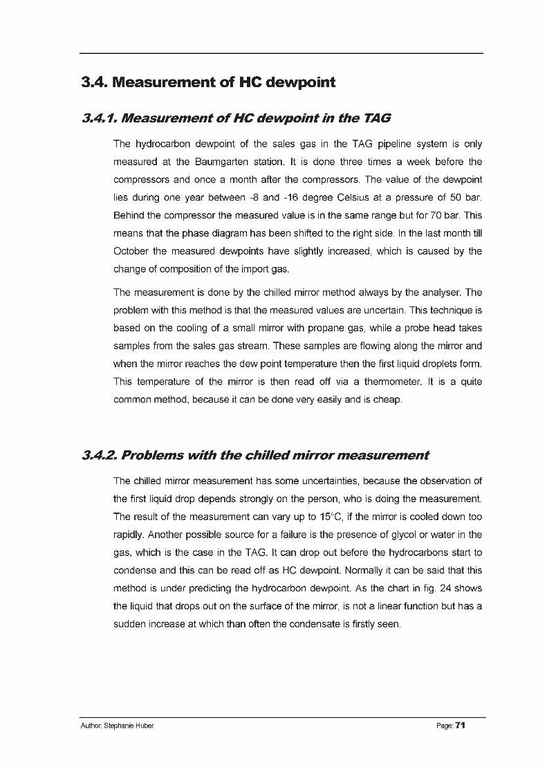
3.4. Measurement of HC dewpoint

3.4.1. Measurement of HC dewpoint in the TAG

The hydrocarbon dewpoint of the sales gas in the TAG pipeline system is only

measured at the Baumgarten station. It is done three times a week before the

compressors and once a month after the compressors. The value of the dewpoint

lies during one year between -8 and -16 degree Celsius at a pressure of 50 bar.

Behind the compressor the measured value is in the same range but for 70 bar. This

means that the phase diagram has been shifted to the right side. In the last month till

October the measured dewpoints have slightly increased, which is caused by the

change of composition of the import gas.

The measurement is done by the chilled mirror method always by the analyser. The

problem with this method is that the measured values are uncertain. This technique is

based on the cooling of a small mirror with propane gas, while a probe head takes

samples from the sales gas stream. These samples are flowing along the mirror and

when the mirror reaches the dew point temperature then the first liquid droplets form.

This temperature of the mirror is then read off via a thermometer. It is a quite

common method, because it can be done very easily and is cheap.

3.4.2. Problems with the chilled mirror measurement

The chilled mirror measurement has some uncertainties, because the observation of

the first liquid drop depends strongly on the person, who is doing the measurement.

The result of the measurement can vary up to 15°C, if the mirror is cooled down too

rapidly. Another possible source for a failure is the presence of glycol or water in the

gas, which is the case in the TAG. It can drop out before the hydrocarbons start to

condense and this can be read off as HC dewpoint. Normally it can be said that this

method is under predicting the hydrocarbon dewpoint. As the chart in fig. 24 shows

the liquid that drops out on the surface of the mirror, is not a linear function but has a

sudden increase at which than often the condensate is firstly seen.


Dustman et al.(36) pointed out that an only experienced technician should make the

chilled mirror analysis. Those people have standard deviations to other methods

between 5 and 10 °C, while an unskilled technician can measure dewpoints, which

differ more than 15°C from calculations.

3.4.3. Other methods for measuring the HC dewpoints

Another possibility for determining the dewpoint of the gas in the pipeline would be a

gas chromatography, which can also detect the smallest amounts of heavy

hydrocarbons and then calculates the dewpoint with and equation of state. The

problem with this method is that also heavy alkanes, which exist only the ppb range,

can influence the dewpoint significantly. A system that can measure this with a good

significance would be very expensive and is probably not available for field

conditions. Therefore this type of equipment is not recommendable for the TAG.

The third method, which can be used for dewpoint determination is the measurement

of the potential hydrocarbon liquid content, which can be correlated to the real dew

point. This method is also quite complicated and expensive for field installations.

Therefore some authors advise an improvement of the first method. This means that

the subjective part of the measurement is substituted by an electro-optical

measurement. There exist methods, which allow measuring the first condensate,


when it is still in the ppm region and thus it is more precise than the normal optical

method.

One very popular method is the dark spot technique. It uses a red light, which is

reflected from a specially treated surface, thus it forms an annulus around a detector,

which is in the dark spot, as it can be seen in fig. 25. This detector measures only the

scattered light that intrudes in this spot. When liquid starts to drop out on this surface

the amount of dispersed light on the detector reduces. When this happens the

temperature of this surface is recognized and this is then the hydrocarbon dewpoint.

This evaluation can be applied to a wide range of different ambient and HCDP

temperatures.

Figure 25: Dark spot principle


3.5. Phase diagrams of the gasFor identifying regions, which are endangered off building liquids, the correct phase

diagram for the gas composition has to be found. This is a very complex problem,

because of the changes of the components at compressor stations, accumulations of

liquid during the transport that changes the overall composition and because of

branches were also the mixture of the gas can be changed.

Therefore three cases were built. The first case includes only the average gas

composition of the sales gas in the TAG and all components above C6 were ignored.

This would be the ideal case for the gas composition displayed in tab. 5 and fig. 26.

COMPONENT %

co2 0.13

n2 0.78

Ci 97.64

c2 0.99

c3 0.32

i-C4 0.05

n-C4 0.06

i-Cs 0.01

n-C5 0.01

c6 0.01Table 5: Ideal gas composition 2


Phase Envelope Best Case

-200 -150 -100 -50 0

Temperature (C)

dew line —- bubble line critical point

Figure 26: Phase diagram: ideal composition

It can be seen easily that out of such a gas liquid cannot drop out under normal

operating conditions. Furthermore it is clear that this is not the normal composition,

because out of hydrocarbon dewpoint measurements, which were in the range of -

8°C and -16°C at a pressure of plus/minus 50 bar.

Out of the information about the HC dewpoints and the composition of the

condensate found, the mixture of the most likely case was built.

3.5.1. K-factors and mole fractions correlation

This correlation was built on the fact that separation of the liquid and the gas has

taken place, when condensate probes are taken to the laboratory and analysed. It is

an unconventional method and should not be extrapolated as general solution.

The so called K-factors can be calculated by the following formula:


Kt=(5.37*(1 + ^. )*(1 - T^1) )

(24)

...acentric factor

TRi ...reduced temperature

pRi ...reduced pressure

For this formula the reduced properties and the acentric factor factors are needed.

For the calculation of the reduced properties the critical properties and standard

temperature and pressure were taken.

The composition of the vapour phase was evaluated by the average of the sales gas

composition till C6+. This was then calculated with the K-factors on the parts which

had to be in the liquid part, but were evaporated due to the fact that the sample box

for the fluids are not gas tight.

(25)

x, ... liquid mol fraction

y, ... vapour mol fraction

The analysis of the C7+ fraction was done with the evaluation of the condensate

composition. Both pieces of information were combined and the values for the

composition of the fluid could now be calculated back with the above mentioned

formula to the gas composition.

The problem with this calculation is that the part of C6 must be estimated, because

neither in the gas composition nor in the condensate analysis the C6 fraction is

directly measured. The estimate was based on the standard correlation described

below.

This analysis leaded to a phase diagram, which is better predicting the measured

hydrocarbon values than that before. All phase diagrams were calculated with GAS


VLE on the basis of the Peng Robinson equation of state and the result is displayed

in tab. 6 and fig. 27.

COMPONENT %

co2 0.13

n2 0.78

Ci 97.63

C2 0.99

C3 0.32

i-C4 0.05

n-C4 0.06

i-C5 0.01

n-C5 0.01

C6 0.01996

C7 1.198E-07

C8 1.2699E-06

C9 5.8702E-07

C10 1.1181E-06

C11 4.3288E-06

C12 7.4715E-06

C13 9.7437E-06

C14 8.4419E-06

C15 4.4725E-06

C16 2.38E-06Table 6: Most likely gas composition

If now the normal operating conditions are introduced into this diagram, it can be

seen that for this most likely case no condensation fluid can be formed. This is also

the experience of the TAG that at most places and fluid is found only seldom.

However, some condensate is found over the whole length of the TAG. Thus there

are only two possibilities how fluids can be formed. One is that the normal operating

conditions are exceeded and the other can be the modification of the gas due to

changes of the input gas composition or by the entrance of heavier hydrocarbons at

the gas compressors.


Phase Envelope Most Likely

s'/

■■

■

-200 -150 -100 -50 0 50

Temperature (C)

-- dew line bubble line critical point

Figure 27: Phase diagram: most likely composition with operating conditions

This variation in the composition leads then to the worst case for the phase diagram.

The oil, which is used at the compressor stations, was analysed and the exact

composition was developed. For building the phase diagram the most likely

composition was taken and the components of the sealing oil. These were evaluated

via gas chromatography. The amount, how much oil must be taken into

consideration, was dependent on the scenario for a single case. There the approach

was that 55 litres of sealing oil is lost into 1.5 million cubic meter of gas. This happens

not during normal working operations of the compressors, but it would be possible for

malfunctions of the sealing unit of one gas compressor.


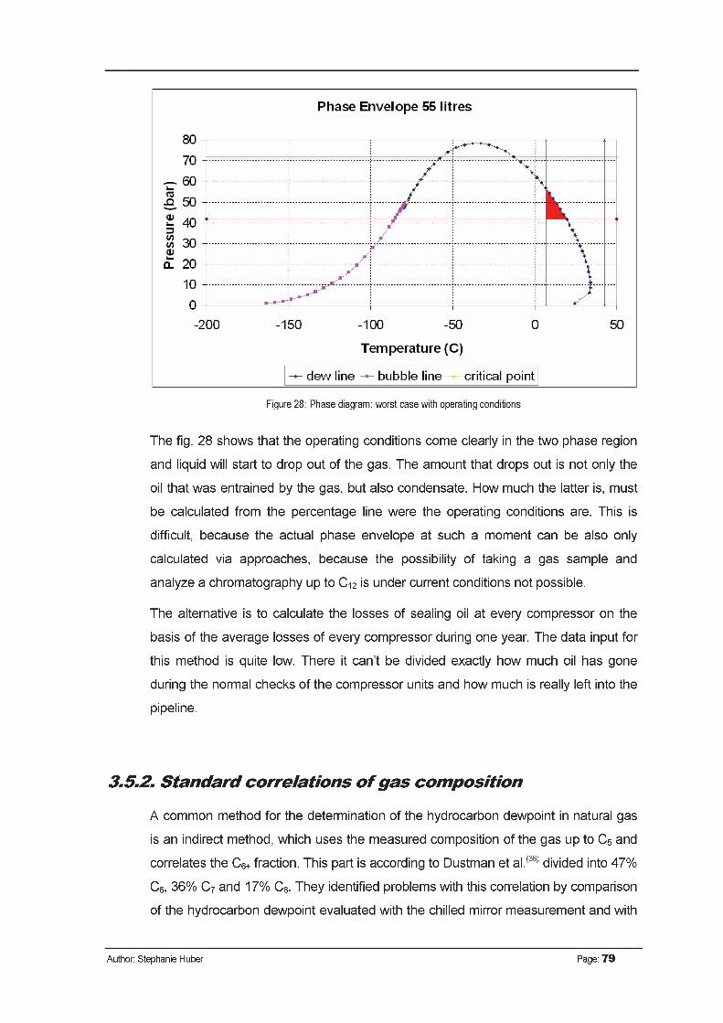
The fig. 28 shows that the operating conditions come clearly in the two phase region

and liquid will start to drop out of the gas. The amount that drops out is not only the

oil that was entrained by the gas, but also condensate. How much the latter is, must

be calculated from the percentage line were the operating conditions are. This is

difficult, because the actual phase envelope at such a moment can be also only

calculated via approaches, because the possibility of taking a gas sample and

analyze a chromatography up to C12 is under current conditions not possible.

The alternative is to calculate the losses of sealing oil at every compressor on the

basis of the average losses of every compressor during one year. The data input for

this method is quite low. There it can’t be divided exactly how much oil has gone

during the normal checks of the compressor units and how much is really left into the

pipeline.

3.5.2. Standard correlations of gas composition

k common method for the determination of the hydrocarbon dewpoint in natural gas

is an indirect method, which uses the measured composition of the gas up to C5 and

correlates the C6+ fraction. This part is according to Dustman et al.(36) divided into 47%

C6, 36% C7 and 17% C8. They identified problems with this correlation by comparison

of the hydrocarbon dewpoint evaluated with the chilled mirror measurement and with


this correlation, because the deviation between both values was up to 15°C. The

result is shown in fig. 29.

Phase Envelope standard correlation

Figure 29: Phase diagram standard correlation

Another method that is often used is the extended gas chromatography. For this

method the gas composition is measured up to C9+ and then the hydrocarbon dew

point is calculated with an equation of state. It was possible to apply this technique for

the actual problem, because a procedure, which was presented in the Erdöl, Erdgas,

Kohle November 2004, was used to determine the heavier hydrocarbons in the gas.

There an adsorption pipe is directly connected to an injection probe head (fig. 30).

Thus the smallest amounts of heavy hydrocarbons can be measured without losses

in a sampling box. Through this adsorption pipe a known amount of gas flew. Thus

the amount of heavy hydrocarbons could be recalculated to a percentage value in

the gas. To get the heavies again out of the pipe desorption process at a defined

temperature was done and then the extracted hydrocarbons were measured with a

gas chromatograph. The accuracy of this measurement was down in the parts per

billion region and resulted in good consistency with the detected hydrocarbon dew

point.


Figure 30: Sampling method for direct measurement in Weitendorfl35)

This procedure was used for this thesis in Weitendorf on 28th November 2007 to

determine the composition of the C6+ fraction. For this case a probe head, which has

reached to the middle of the gas stream, placed after the filter separator of the

branching point of the Sol, was used to take the sample of the gas. Therefore the

measured amount of 15 litres gas flowed through an adsorption pipe filled with

activated charcoal. Additionally the water dewpoint and the hydrocarbon dewpoint

were measured with the above described method of chilled mirror. There existed

problems for the evaluation of the HC dewpoint, because at 61 bar the condensation

on the mirror could not be identified with 100 % as condensate. For this reason the

pressure was reduced for a further measurement and at 30 bar hydrocarbon

condensate could be found. The ambient temperature was determined and also the

temperature of the gas. Furthermore two dry and two wet samples of the gas were

taken for the determination of the gas composition.

The results of the measurements are the displayed in tab. 7 and tab. 8:

water dewpoint -13°C at 61 bar

HC dewpoint -13 °C at 30 bar

gas temperature 26.6 °C at 61 bar

ambient temperature 5 °CTable 7: Measured data


Component: mol %

CO2 0.1827

n2 0.8012

ch4 97.4380

C2H6 1.1012

C3H8 0.3455

I-C4H10 0.0494

N-C4H10 0.0555

I-CsHi2 0.0102

n-c5h12 0.0073

C6H14 0.0056

C7H16 0.0021

C8Hi8 0.0010

CgH2o 0.0001

mol-weight [kg/kmol] 16.4993

density [kg/m3] 0.7375Table 8: Measured composition

It was not possible to determine also the heavier hydrocarbons, because the

sampling and measurement devices, which can be applied, are not accurate enough

to receive trustable results in the ppm region.


The phase envelope is built with the analysis up to C9. It can be seen in fig. 31 that

the measured value of the HC dewpoint is far away from the one built with Gas VLE.

There are two possible explanations for this difference.

The first is that during the measurement the two dewpoints were close together.

Therefore it is possible that the hydrocarbon dewpoint was confused with the water

dewpoint. This is likely, if the dewpoint is as low as the calculation shows.

The other explanation is that there still exist heavier hydrocarbons in the gas, which

would influence the calculation of the dewpoint significantly. Therefore it is necessary

to model the possible composition of this part of the gas. The first method used, is to

apply the normal standard correlation to the Ci0+ values. This leads to the result

showed in figure 35. As it can be seen in fig 32 the hydrocarbon dewpoint is far away

from measured results. Therefore this method is not appropriate.


Phase Envelope 1. correlation

\

■■ \)

-200 -150 -100 -50 0

Temperature (C)

-- dew line —- bubble line critical point

Figure 32: Phase diagram 1. correlation

The second model, which is applied, uses the same distribution of the heavier

hydrocarbons as the model, which has been developed for the most likely scenario

distribution.

However, this model now is over predicting the measured hydrocarbon dewpoint

significantly (fig. 33). This can be on the one hand due to the effect of the

hydrocarbon tail for the measurement, or that some additional hydrocarbons have

already dropped out, that changed the composition of the heavier hydrocarbons and

therefore the hydrocarbon dewpoint decreased.


Phase Envelope 2. correlation

Temperature (C)

-- dew line —- bubble line critical point

Figure 33: Phase diagram 2. correlation

Based on this analyses it can be said that the real phase diagram of the composition

must lay in between the direct measurement and the second correlation for normal

gas flow. At this point the influence of the lubricating oil from the compressor on the

composition can be already neglected, because the resulting condensates are

normally formed directly after the compressors. Only by reentrance into the gas they

can have an influence, but directly at this branching system no condensates are built.

3.5.3. Liquids built due to pressure and temperature variation

The pressure downstream from branching systems is normally lower than upstream.

The reduction is performed at this point. Regular decreases are between 5 and 10

bar. If we calculate the Joule-Thomson coefficient for a maximum temperature of

25°C, which is the minimum coefficient, then we get a result of 0.33 K/bar. For lower

temperatures the coefficient increases till 0.4 K/bar.

Therefore the maximum temperature reduction at the delivery point can be 4°C.

Further pressure decreases will lead to more temperature reduction. Thus it is

possible that with both incidents at the same time the operating conditions reach the

two phase area and additional fluid is created right after the delivery point. An

additional contribution can be a lower temperature of the gas.


3.5.4. Maximum amount of condensates as aerosols at the branching point Weitendorf

Since the installation of the filter separator in Weitendorf one year ago the amount of

fluid, which was found, had a total amount of 15 litres. The filter is able to remove

99.9% of the aerosols, which are large than 1 pm. Therefore the amount of liquid

aerosols sized larger than this, which are able to pass the filter, is 0.015 litres. As it is

shown before normally 80 percent of the aerosols are larger than one micrometer.

Thus twenty percent are smaller and can also bypass the filter. The volume of these

aerosols is 3.75 litres. Therefore it can be said that not more than 4 litres in one year

are bypassing this filter. The rest of the liquid, which is found in the pipelines after the

branching point, must be built through the reduction of the pressure and temperature

in this system.


3.6. Glycol vapour pressure analysisThe aqueous mixture of TEG and DEG can have only entered the pipeline system

during the flow of the gas through an absorber tower. There is normally installed a

demister after the bubble trays to avoid glycol losses into the line, but during normal

operating conditions it is possible that they are going through this due to the fact that

some of the TEG becomes vaporized.

There are two possibilities why not only triethylene glycol is found in the sample but

also DEG. The first is that the TEG was converted through thermal reduction into

DEG and the other is that some DEG is transported from Russia to Austria via the

transit pipelines, because in Austria DEG is not in use any longer, because its vapour

pressure is higher and therefore more glycol would be lost into the line. Furthermore it

would not decrease the water dewpoint of the gas as much as the TEG.

The vapour pressures of diethylene glycol were evaluated on the basis of the

Ambrose Walton method. It uses the critical data of the substance and its acentric

factor for the calculation.

The acentric factor is a parameter that shows how much like a sphere is the shape of

the molecule of a substance. It is calculated with the following formula:

®= 7* *lo«|-£L|-1 <2S>7 Tc - Tb p0 J

w.. .acentric factor

TB...normal boiling temperature [K]

Tc...critical temperature [K]

pc... critical pressure [bar]

po=1.O13 bar

The equations of the Ambrose Walton method itself:

In I I = f(0) + ® * f(1) + ®2 * f(2) (27)


(0)

(1)

(2)

-5,97616*r + 1.29874*rk5 -0.60394*rZ5 - 1.06841*r5

Tr

-5.03365*r + 1.11505*?-5 -5.41217*rZ5 -7.46628*r5

Tr

- 0.64771 * r + 2.41539 * ?-5 - 4.26979 * r2'5 + 3.25259 * r5

Tr

(28)

z.Tc

T = 1 - Tr

Tr...reduced temperature

(29)

(30)

(31)

(32)

f

f

f

T =

The values for diethylene glycol were taken from the nist chemistry web book and

displayed in tab. 9.

This data leads to the amount of diethylene glycol, which can evaporate at a certain

temperature and pressure. This is then the maximum amount of glycol that can be in

gas phase and will flow with the sales gas into line. The results of the calculation are

in Appendix A.

critical temperature Tc 753 [K]

critical pressure pc 47.7 [bar]

boiling temperature at 1.013 bar Tb

515.15 [K]

Table 9: Triethylene glycol data

The uncertainty for this calculation was that diethylene glycol will be not used as 100

percent pure substance, but as a mixture of water and glycol due to the fact that the

Ambrose Walton method was developed for pure substances.

The vapour pressures of triethylene glycol were evaluated by the Antoine equation,

which can be used when the constants are known. The values for the calculation

were delivered by the chemistry company DOW.

The Antoine constants for triethylene glycol are shown in tab. 10:


TEG weight % A B C

0 7.959199 1663.545 227.575

50 7.922294 1671.501 228.031

70 7.878546 1681.363 228.237

80 7.837076 1697.006 228.769

90 7.726126 1728.047 229.823

95 7.620215 1806.257 236.227

97 7.495349 1841.522 238.048

98 7.404435 1881.474 240.666

99 7.211145 1926.114 242.799

99,5 7.042989 1970.802 242.865

100 7.472115 2022.898 152.573TablelO: TEG glycol data

The Antoine equation is the following:

ßlog10(A> = A - ? + c(33)

p... pressure [Torr]

T... temperature [°C]

Inserting the constants into the equation leads to the vapour pressure of TEG and

the results can be found in Appendix A. The calculation of the vapour pressures

leads to the information how much glycol can be in vapour phase at a certain

pressure and temperature. Therefore it is possible to evaluate how much glycol starts

to condense.

The worst case scenario for this case would be new glycol, which has a water part,

which tends to be zero. The normal aqueous part of TEG in OMV dehydration units is

below 2 %, but when new glycol is filled in this part decreases. Normally the absorber

units have to be refilled during the start up process, because the regulators of the

dehydration units have some failures in this period. Therefore the guaranteed value

for the losses at the absorber tower, which is normally less than 6 kilogram per

1,000.000 standard cubic meters, are exceeded during this process. Then maximum

losses can be up to 1300 litres in 3 days according to the engineers, which are

responsible for the start up. The glycol dehydration units are not active during the


year. Only when the water dewpoint increases above -6 °C, the absorber towers dry

the gas. In the year 2007 the dehydration units were unusual often actuated. In the

months August and October the glycol units were already activated in each case for

one week.

The minimum amount of gas, which flows in three days in the TAG would be 26.7

million cubic meter gas and the maximum would be 101.1 million cubic meter. The

worst case would be that a minimum of gas flows through the absorber towers, while

they are started. This would mean that the 1300 litres would be dispersed in 26.7

million cubic meter gas. If this is calculated back to 1 million cubic meter gas, this

would mean that in every million m3 gas 48.7 litres glycol are dispersed. The vapour

pressure in the worst case for a 99.5 % pure TEG would be dependent on the current

total pressure far below this.

In the worst case scenario the gas would be cold, which means a temperature

around ten degrees Celsius. The purity of the TEG would be high, as suggested here

99.5 % and also the total pressure would be high, so it is taken for the calculation as

the highest possible with 70 bar. All these assumptions leads to a possible amount of

glycol that stays in vapour phase with only 0.00201 litres per 1 million cubic meter

gas.

Due to these facts the largest amount of TEG which can be taken for the analysis of

the flow regime is 48.687 l/million m3gas.

The calculation how much diethylene glycol can condense is more complicate then

evaluation of TEG, because it is not possible to say how much DEG is left in the gas

after the transport. Therefore it is necessary to draw the conclusion that DEG will

react in the same way as the TEG and in the worst case will drop out not more DEG

than TEG.

Thus the maximum amount of aqueous glycol will not be more than 100 litres per 1

million cubic meters of gas.


3.7. Analysis of flow regime in the TAGFor the analysis of the flow regime the author used the method after Ben Asante,

because this model was especially developed for the flow of transmission gas with

only low liquid loads.

v(34)

(„ \ °-51W rrr . < 1 +10.4* Re 5L0363*-1 [

USGk

VPc, J(35)

?7 L>

The measured viscosity of the liquid, which consisted of condensate and lubrication

oil, was the following:

vl=83.438 mm2/s and q= 72.333*10’3 Pas at 20°C

vl=49.25 mm2/s q= 42.402*10’3 Pas at 30°C

vl=31 .244 mm2/s q= 26.697*10’3 Pas at 40°C

The density of the fluid was also determined:

p=866.9kg/m3 at 20°C

p=861 kg/m3 at 30°C

p=854.5kg/m3 at 40°C

The values for the constant parameters of TEG were calculated by values, which

were listed by the chemistry company DOW and evaluated with equation 37 and

displayed in tab. 11 and fig. 34.


7 = A :;:IO (37)

q...viscosity [cP]

x...weight % of TEG

Temp. [°F] A B

0 1.53010 2.9967E-2

50 1.09200 1.9348E-2

100 0.58916 1.5763E-2

150 0.37045 1.3481E-2

200 0.27371 1.1731E-2

250 0.18759 9.7064E-3

300 0.14026 8.1319E-3Table 11: Triethylene glycol viscosity constants

viscosity of 99,5 % TEG

[-»-vise. Of 99,5% TEG |

Figure 34: Viscosity of 99.5 % TEG

The viscosity is only slightly changing with varying water content of the TEG, thus the

modification of the values are so small that they are negligible.

For the calculation of the velocity the diameter of the pipe and the amount of gas that

is flowing through the pipe is necessary. Then the amount of liquid that flows at the


maximum and with the most likely probability can be evaluated via the quality lines of

the phase diagrams and additionally the glycol amount must be calculated.

The amount of gas that flows through the system is only measured in the TAG 1 and

must be calculated back to all three pipelines. Due to the fact that the three pipes

have very similar diameters it is possible to say that nearly one third of the amount is

flowing through each pipe. The significant points of interest are the compressor

stations and the offtake points along the pipeline. These are the places, where it is

important to know, do I have fluid in the gas and in which flow regime is it.

A...pipe area [m2]

d...pipe diameter [m]

qL...liquid amount [m3/day]

vL...fluid velocity [m/day]

Therefore the cross section in TAG 1 from Baumgarten to Grafendorf can be

evaluated as 0.69 m2 after Grafendorf to Wettmannstetten with 0.689 m2 and behind

Wettmanstetten to Rüden the area is calculated with 0.620 m2. The pipe between

Rüden and Arnoldstein has an area of 0.618 m2.

The TAG 2 also consists of pipes with different diameters. Therefore the area from

Baumgarten to Grafendorf is only 0.842 m2 and afterwards till Arnoldstein 0.843 m2.

The TAG Loop 2 (TAG 3) is built in one dimension over the whole length and hence

the pipe area is 0.771 m2.

The exact amount of fluid, which flows in the gas stream at every point, can not be

determined, because the composition of gas changes all the time and therefore the

amount of fluid. Furthermore the operation conditions are variable, which makes it

impossible to determine the exact amount of fluid everywhere. Therefore it is

necessary to say what the maximum liquid content of the gas would be and what the

consequent flow regime is.


The sum of TEG and DEG is in the maximum case 100 litres per one million cubic

meter gas. Lubrication oil is lost at maximum 20 000 litres per year, whereas the main

portion does not go into the pipeline, but is changed during maintenance. Therefore

only 20 % of this value can be taken for this calculation. This means 4000 litres in 4

billion cubic meter gas per year. When this is calculated back, we must add 1 litre per

one million cubic meter gas as an average. However, the technicians at the

compressor stations mean that for singular occasions also values of up to 50 litres

per one million cubic meter gas can be reached. Out of the K-factor analysis we

know that the maximum liquefiable part of the gas is 0.1 ppm, when we take the most

likely composition. This means 100 litres per one million cubic meter gas. Hence the

total amount of fluid in the worst case would be 250 litres/MMCM. The minimum gas

amount that flows in the TAG is 26.5 million cubic meter per day.

This means for the calculation in Weitendorf an area that consists of the following

parts:

TAG 1 Grafendorf to Wettmannstetten 0.689 m2

TAG 2 Baumgarten to Grafendorf 0.842 m2

TAG Loop 2 (TAG 3) 0.771 m2

ZA=2.302 m2

0.1m

_ ylycol(24*3600)

2.302

!. condensate

m= 0.00181 [ ] = 5.003*10]

h sec

0.15 _ (24*3600) _ “ 2.302

Ml 77?

= 0.002715[ ] = 7.54*10 ) ]h sec

Condensate plus lubrication oil:

q= 72.333*10‘3 Pas

p=866.9kg/m3 at 20°C

DEG 20°C: viscosity: 38 mPas density: 1120 kg/m3

TEG 20°C: viscosity: 49 mPas density: 1124 kg/m3


average: viscosity: 43.5 mPas density: 1122 kg/m3

ReSL condensate866,9*7,54*10’7 *1,712

72.333*10 ;= 1.55*10

ReSLglycol

1122*5.003*10 *1.712 43.5*10

= 2.21*10

SG

qG _ 111070.9 msec

=^- =------------ = 13,4[----- ] vL = uSLA 2.302

7.54*10condensate 13.4

*h +10.4 * (1.55 *10d’°'363 * 866,90.7375

,0.5

> = 9.11*10 -5

' L condensate9,11*10

(1 + 9.11*10 "')= 9.11*10"

glycol

5,003*1013.4

< 1 +10.4*(2.21*10’2)’°-363 *1122

0.7375

.0.5

= 6.045*10’5

6.045*10(1 + 6.045*10’5)

■ = 6.046*10

SL total SL + Fcondensate L _ yivcoi = 9.11*10 ’5 + 6.046*10 ’5 = 1.516*10’

total < 0.005

' L _ ylycol

sL

-

1

-

For the calculation the maximum amounts of liquid were taken and the minimum

amount of gas. The evaluation was done for the TAG mainstream, but it is also valid

for the branching arms, because the amount of aerosols, which flow into a branching

arm, is proportional to the gas amount. The viscosity and density values were taken

at the average temperature of 20°C.


3.8. Vanishing of liquidThe liquids and accumulations in the pipeline systems are not constant. Therefore it

can happen that at one point sometimes fluid can be found and the next time

everything is dry. The causes for these events are diverse.

One is that the operating conditions are changing when the surrounding temperature

varies, compressor stations go offline or something else happens, which changes

either the temperature or the pressure of the gas.

Another reason is that also the composition of the sales gas is not constant. There

exist only guideline values, which restrict minimum and maximum values of the single

components. This is critical for the heavy hydrocarbons, where normally only the total

amount of the C6+ values is regulated, while it is of the same importance, how they

are distributed. These distributions are of such sensibility that variations in the ppm

region and below are enough to make the difference between the possibility that

liquids build or not.

Due to the fact that during the start up phase also triethylene glycol is lost into the

pipeline, while in most times of the year no glycol drying is necessary, also the

amount of glycol in the system is permanently changing. Furthermore the amount of

sealing oil, which gets lost at the compressors, is not always the same. During normal

operation the losses are nearly negligible, but when failures occur the amount can

rise to 55 litres per million cubic meter gas in a short period.

When liquid really condenses, it can travel around 700 meters, before accumulation

starts. On the one hand these puddles of fluids can re-vaporise into the gas phase

when the composition or the operating conditions change, because then the vapour

pressure above the liquid also changes. On the other hand the fluid at the bottom of

the pipe is entrained because of the high velocity of the gas. This means values

around 15 m/s.


3.9. Technical Consequences and possible solutionsThe conclusion out of the analysis made is that in the TAG pipeline systems not only

single phase flow occurs, but also mist flow with aerosols is possible. The exact

points, when the transition happens cannot be predicted properly due the continuous

change of the operating conditions.

A result of this research is that parameters were find, which contribute to the affinity

of the gas to build liquids. One of it is the amount of lost sealing oil at the compressor

stations. To minimize this parameter the possibility of changing the sealings from oil

based to dry ones, should be taken into consideration. This would decrease the

amount of heavy hydrocarbons and can therefore reduce the dewpoint of the gas.

Thus the condensation of hydrocarbons from the gas would be less and also the

amounts of the sealing oil would be less. It would be advisable to monitor at the

compressor stations, how much oil is left to the pipeline and how much is changed at

the normal inspection, before such a project can be done.

The glycol, which is also part of the fluids, comes on the one hand from the import

gas itself and on the other hand from the drying units in Baumgarten. The first point

can’t be changed; hence an analysis for the improvement of the drying unit operation

should be made. How much glycol gets lost by carry over to the system and is it

possible to reduce this by the change of the start up operation.

It is clear that the dewpoint of the gas changes with pressure, temperature and the

influence of the heavy hydrocarbons. Although the gas can be clean of fluids at the

delivery point, the possibility of liquid generation somewhere behind this point can’t

be excluded. For this reason it must be suggested that sensible customers protect

their equipment by their own separation systems.


4. References1. Parker C. Reist, Introduction to aerosol science, MacMillan, New York, 1984

2. Pruppache H. F., Klett J. D., Microphysics of Clouds and Precipitation, Springer,1996

3. Kruis F. E., Küster K. A., The collision rate of particles in turbulent media, Journal of Aerosol Science Vol. 27, S.263-264, 1996

4. Schmidt F., Transport und Abscheidung submikroner Partikel, Gerhard Mercator Universität Düsburg, Habilitationsschrift, 2001

5. Fan F.-G., Ahmadi G., A sublayer model for turbulent deposition of particles in vertical ducts with smooth and rough surfaces, Journal of Aerosol Science, Vol. 24, Nr.1, S.45-64, 1993

6. Sager C., Der Partikeltransport in turbulent durchströmten Rohrleitungen und seine besondere Bedeutung für die Partikelmesstechnik, Universität DüsburgEssen, Dissertation, 2007

7. Friedlander S. K., Smoke, Dust and Haze, John Wiley & Sons, New York, 1977

8. Hope, P.M., Nelson R. G., A new approach to the design of wet gas pipelines, ASME conference, Houston, 1997

9. Asante Ben, Multiphase transport of gas and low loads of liquids in pipelines, University of Calgary, dissertation, 2000

10. Adewumi M. A., Boriyantoro N. H., An integrated single-phase/two -phase hydrodynamic model for predicting the fluid flow behaviour of gas condensate pipelines, The Pennsylvania State University

H.Griston S., Choi J. H., Two phase flow splitting at side-branching tees, SPE46237, SPE Western Regional Meeting, California, 1998

12. Baker G., Clark W. W., Azzopardi B. J., Wilson J. A., Controlling the phase separation of gas-liquid flows at horizontal T-junctions, Wiley Interscience, AiChe, 2007

13. Putra S. A., East Javagas pipeline liquid condensation study using dynamic multiphase flow simulator, SPE 77928, SPE Asia Pacific Oil and Gas Conference and Exhibition, Australia, 2002

14. Adewumi M. A., Mucharam L., Compositional multiphase hydrodynamic modelling of gas/gas-condensate dispersed flow in gas pipelines, SPE 17056, SPE Eastern Regional Meeting, Pittsburgh, 1987

15. Sadegh A. A., Adewumi M. A., Temperature distribution in natural gas/condensate pipelines using a hydrodynamic model, SPE 97978, SPE Eastern Regional Meeting, Morgantown, 2005

16. Adewumi M. A., Mucharam L., A compositional two phase flow model for analyzing and designing complex pipeline network systems, SPE 21562, SPE International technical meeting, 1990

17. Adewumi M. A., Nor-Azlan N., Tian S., Design approach accounts for condensate in gas pipelines, SPE 26904, SPE Eastern Regional Conference and Exhibition, Pittsburgh, 1993


18. Verloo E., Belval S., Saldo V., Albiol T., Sabathier F., Study of aerosol deposition in larger pipes: Transat programme, Journal of Aerosol Science, Vol. 27, Nr.1, S.453-454, 1996

19. Adewumi M. A., Mucharam L., Watson R. W., Field study and modelling of condensation in a gas distribution pipeline, SPE 19811, 64th Annual Technical Conference and Exhibition of SPE, San Antonio, 1989

20. Martinez F. F., Adewumi M. A., Two-phase gas-condensate flow in pipeline opennetwork systems, SPE 30995, SPE Eastern Regional Meeting, Virginia, 1995

21. Schmidt F., Sager C., Deposition of particles in turbulent pipe flows, Journal of Aerosol Science, Vol. 31, Nr.1, S.847-848, 2000

22. Ahmadi G., Chen Q., Dispersion and deposition of particles in a turbulent pipe flow with sudden expansion, Journal of Aerosol Science, Vol. 29, Nr.9, S.1097- 1116, 1998

23. Ahmadi G., Chen Q., Deposition of particles in a turbulent pipe flow, Journal of Aerosol Science, Vol. 28, Nr.5, S.789-796, 1997

24. Romay F. J., Takagaki S. S., Pui D. Y. H., Liu B. Y. H., Thermophoretic deposition of aerosol particles in turbulent pipe flow, Journal of Aerosol Science, Vol. 29, Nr.8, S.943-959, 1998

25. Tandon P., Adewumi M. A., Particle deposition from turbulent flow in a pipe, Journal of Aerosol Science, Vol. 29, Nr.1/2, S.141-156, 1998

26. Campbell J. M., Gas conditioning and processing, Volume 2: The equipment modules, John M. Campbell and Company, Oklahoma USA, 2001

27. Spumy K. R., Advances in aerosol filtration, Lewis Publishers, Florida USA, 1998

28. Reist P. C., Introduction to aerosol science, Macmillan Publishing Company, New York USA, 1984

29. Erhärt D. L., Turbulent aerosol deposition and reentrainment, University of California, Berkeley, dissertation, 1986

30. Ilory, T. A., Turbulent deposition of aerosol particles inside pipes, University of Minnesota, dissertation, 1971

31. Gallily I., Transport mechanics of aerosols - nonspherical particles, Academon LTD. Printing and Publishing House, The Hebrew University of Jerusalem, 2001

32. Crane R. I., Evans R. L., Inertial deposition of particles in bent pipes, Journal of Aerosol Science, Vol. 8, S.161-170, 1977

33. Schulze K., Menzel W., Kleinitz W., Sewe K.-U., Eiden R., Busch M., Determination of concentrations of higher hydrocarbons in natural gas and associated gas, Erdöl Erdgas Kohle, Heft 11, 2004

34. Colbeck I., Physical and chemical properties of aerosols, Blackie Academic and Professional, The University of Essex, 1998

35. White paper on liquid hydrocarbon dropout in natural gas infrastructure, Natural Gas Council for the Federal Energy Regulatory Commission, NGC+ Liquid Hydrocarbon Dropout Task Group, October 2004

36. Dustmann T., et al., An analysis and prediction of hydrocarbon dew points and liquids in gas transmission lines, Tulsa Oklahoma, GPA 2006


37. Ho Chi Ahn, Modellierung der Partikelagglomeration im Rahmen des Euler/Lagrange-Verfahrens und Anwendung zur Berechnung der Staubabscheidung im Zyklon, Dissertation, Universität Halle, 2004

38. Pinsky, M. B., Shapiro M., Collisions of small drops in a turbulent flow. Part I: Collision efficiency: Problem formulation and preliminary results. J. Atmos. Sei., 56, 2585-2600, 1999

39. Pirker, B., Übungen zu Erdöl- und Erdgasproduktionstechnik 2, 2006

40. Ambastha, A. K., Gudmundson, J. S., Geothermal two phase wellbore flow: pressure drop correlations and flow pattern transition, Stanford Geothermal Program Workshop Report,1986

Author: Stephanie Huber Page: 1OO

5. Appendix A

Amount Glycol [I]

temperatureat 30 bar at 40 bar at 50 bar at 60 bar at 70 bar[K] temp [°C]

263,15 -10.00 0.00008 0.00006 0.00005 0.00004 0.00004

273,15 0.00 0.00072 0.00054 0.00043 0.00036 0.00031

283,15 10.00 0.00469 0.00352 0.00281 0.00234 0.00201

293,15 20.00 0.02467 0.01850 0.01480 0.01234 0.01057

303,15 30.00 0.10820 0.08115 0.06492 0.05410 0.04637

313,15 40.00 0.40701 0.30526 0.24420 0.20350 0.17443

323,15 50.00 1.34 1.01 0.81 0.67 0.58

333,15 60.00 3.96 2.97 2.38 1.98 1.70

343,15 70.00 10.60 7.95 6.36 5.30 4.54

353,15 80.00 26.08 19.56 15.65 13.04 11.18

363,15 90.00 59.54 44.66 35.73 29.77 25.52

373,15 100.00 127.36 95.52 76.41 63.68 54.58Table 12: Maximum amount of vap. triethylene glycol in litre per 1 mill, m3 gas

Vapour pressure TEG

-»-100% TEG —■—99,5% TEG 99% TEG -* 98 % TEG —*—97% TEG —«—95% TEG —1—90% TEG —80% TEG 70% TEG 50% TEG 0% TEG

Figure 35: Calc, vapour pressure of TEG


oCL

Vap. Press. TEG 2

0,0000012

0,000001

■=* 0,0000008 n 0)

ÜÖ0,0000006

0,0000004

0,0000002

0 5 10 15 20 25 30 35 40

temperature [°C]

•TEG 100% -»-TEG 99,5%

Figure 36: Calc, vapour pressure of TEG 2

temperature[K]

temp[°C] at 30 bar at 40 bar at 50 bar at 60 bar at 70 bar

263.15 -10 0.1007 0.0756 0.0604 0.0504 0.0432

268.15 -5 0.1924 0.1443 0.1154 0.0962 0.0825

273.15 0 0.3573 0.2680 0.2144 0.1787 0.1531

278.15 5 0.6464 0.4848 0.3879 0.3232 0.2770

283.15 10 1.1407 0.8555 0.6844 0.5704 0.4889

288.15 15 1.9663 1.4747 1.1798 0.9832 0.8427

293.15 20 3.3152 2.4864 1.9891 1.6576 1.4208

298.15 25 5.4734 4.1050 3.2840 2.7367 2.3457

303.15 30 8.8590 6.6442 5.3154 4.4295 3.7967

308.15 35 14.0715 10.5536 8.4429 7.0357 6.0306

313.15 40 21.9558 16.4668 13.1735 10.9779 9.4096

318.15 45 33.6828 25.2621 20.2097 16.8414 14.4355

323.15 50 50.8497 38.1373 30.5098 25.4248 21.7927

328.15 55 75.6023 56.7017 45.3614 37.8012 32.4010

333.15 60110.783

7 83.0878 66.4702 55.3918 47.4787

338.15 65 160.109 120.0819 96.0655 80.0546 68.6182


2

343.15 70228.373

1 171.2798 137.0238 114.1865 97.8742

348.15 75321.686

2 241.2646 193.0117 160.8431 137.8655

353.15 80447.748

5 335.8113 268.6490 223.8742 191.8922

358.15 85616.155

6 462.1166 369.6933 308.0777 264.0666

363.15 90838.741

5 629.0560 503.2447 419.3706 359.4605

368.15 951129.95

5 847.4664 677.9730 564.9775 484.2664Table 13: Maximumamountofvap. diethyleneglycol in litre

Vapour pressure DEG

Figure 37: Calc, vapour pressure of DEG

TAG1pres, min [bar] pres, max [bar] temp, min [°C] temp, max [°C]

Baumgarten 51.64 69.18

Eggendorf 49.27 67.87

Eggend. EVN 45.53 56.52

Grafend, vor K. 42.52 64.87 8.88 18.49


Grafend, n. K. 54.43 70.31

Graf. BEGAS 41.62 60.01

St. Marg. 52.53 69.01

St.Marg.STGW 17.97 66.76

Weitendorf

Weitd. STGW 46.12 59.31

Weitd. SOL 49.95 66.72

Sulm.-Gr. 49.87 67.77

Sulm.-Gr.STGW 47.94 65.54

Ettendorf 45.63 66.66

Ettend. KELAG 7.98 62.48

Rüden vor K. 42.17 65.49

Rüden nach K. 58.7 69.82

Waisenberg 46.05 70.89

Waisenb.KELAG 44.9 67.29

Ebenthal 58.48 68.71 1

Eben. KELAG 58.48 66.66

Finkenstein 54.77 67.59

Fink. KELAG 29.15 64.37

Arnoldstein

TAG2pres, min [bar] pres, max [bar] temp.


Eggendorf 48.69 67.37

Eggend. EVN

Grafend, vor K. 42.59 65

Grafend, n. K. 54.43 70.31

Graf. BEGAS

St. Marg. 0 69.49

St.Marg.STGW

Weitendorf 51.33 68.58

25.23

temp, max [°C]


Weitd. STGW

Weitd. SOL

Sulm.-Gr.

Sulm.-Gr. STGW

Ettendorf

Ettend. KELAG

Rüden vor K.


Waisenberg 58.82 69.27

Waisenb.KELAG

Ebenthal 54.88 69.03

Eben. KELAG

Finkenstein 56.13 67.63

Fink. KELAG

Arnoldstein 54.08 66.14

TAG3pres, min [bar] pres, max [bar] temp, min [°C] temp, max [°C]


Eggendorf 48.59 67.35 15.88 26.12

Eggend. EVN

Grafend, vor K.

Grafend, n. K.

Graf. BEGAS

0.02

54.43

65.11

70.31

St. Marg. 1.64 69.2 12.17 29.93

St.Marg.STGW

Weitendorf 52.07 71.61

Weitd. STGW

Weitd. SOL

Sulm.-Gr.

Sulm.-Gr.STGW


Ettendorf

Ettend. KELAG

Rüden vor K.


Waisenberg 58.63 69.58 15.19 39.72

Waisenb.KELAG

Ebenthal 58.37 73.11

Eben. KELAG

Finkenstein 0 65.01 6.93 42.57

Fink. KELAG

Arnoldstein 11.72 19.11

Table 14: Minimum and maximum data for the offtake points and compressor station


Date post:	28-Feb-2019
Category:	Documents
Upload:	tranthuy
View:	213 times
Download:	0 times

Aerosols in gas transporting systems - pure.unileoben.ac.at · Figure 10: Orkiszewski flowpattern...

Documents