Abstract The aerothermodynamic characteristics ofthe Brazilian satellite Satélite de Reentrada Atmosféricawere calculated for orbital-flight and atmospheric-reentry conditions with the direct simulation MonteCarlo method for a diatomic gas. The internal modes ofmolecule energy in the intermolecular interaction, suchas the rotational energy, were taken into account. Thenumerical calculations cover a range of gas rarefactionswide enough to embrace the free-molecule and hydro-dynamic regimes. Two Mach numbers were considered:10 and 20. Numerical results include the drag force ofthe satellite, the energy flux, pressure coefficient, andskin friction coefficient over the satellite surface, thedensity and temperature distributions, and streamlinesof the gas flow around the satellite. The influence ofthe satellite temperature upon these characteristics wasevaluated at different satellite temperatures.
Keywords Aerothermodynamics · DSMC ·Rarefied gas dynamics · Satellite
1 Introduction
The project of a recoverable satellite must solve twoproblems concerning rarefied-gas flow. To compute
D. V. Kozak (B)Departamento de Engenharia da Computação,Pontifícia Universidade Católica do Paraná,Curitiba, Paraná,Brazile-mail: [email protected]
F. SharipovDepartamento de Física, Universidade Federal do ParanáCaixa Postal 19044, Curitiba, 81531-990, Brazil
trajectories, one must know the drag forces on thesatellite. And to design adequate heat protection, oneneeds information about the heat flux to the satellitesurface. These problems are usually referred to as theaerothermodynamics of space vehicles [1–4].
In the upper levels of the atmosphere, the mean freepath of gaseous molecules is of the order of severalmeters. Under such conditions, the gas flow can betreated as free molecular, i.e., one can neglect theintermolecular collisions to calculate the aerothermo-dynamic characteristics. The continuum hypothesis isinvalid, and the equations of continuum mechanics be-come inapplicable.
At lower levels of the atmosphere, the satellite speedis still high, in the hypersonic regime, and althoughthe atmosphere can be viewed as a continuum, thecontinuum equations are still difficult to handle be-cause the density changes around the satellite are solarge that regions of rarefied flow can be present [5].Special treatment is moreover necessary because themolecules can dissociate and recombine in hypersonicflow. One must then turn to the methods of rarefied-gas dynamics, which can be divided in two large groups.In the first group are methods based on the kineticBoltzmann equation [6–10], while the second groupcomprises approaches based on the direct simulationMonte Carlo (DSMC) method [11].
While requiring greater computational efforts, thesecond approach is more suitable for practical appli-cations because the program can be easily generalizedto polyatomic gases and gaseous mixtures. This is veryimportant, since in practice one deals with the air, amixture of polyatomic gases.
The present paper extends the work of Sharipov[12], which was restricted to a monatomic gas. The
Braz J Phys (2012) 42:192–206 193
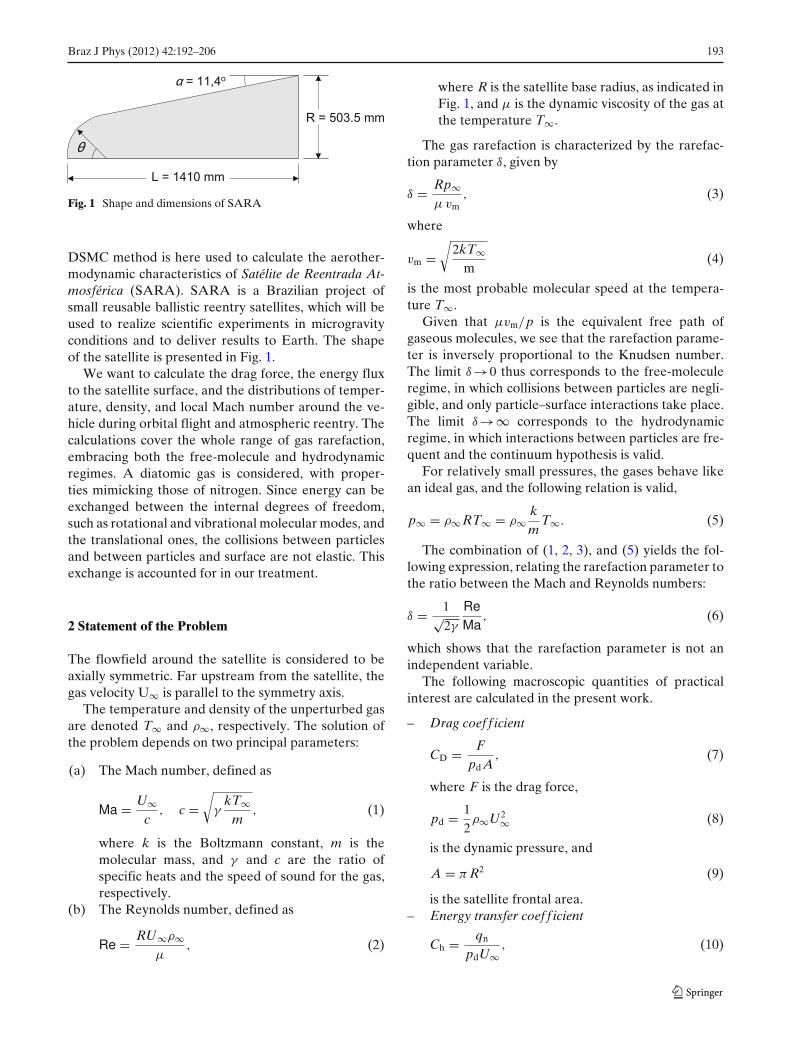
Fig. 1 Shape and dimensions of SARA
DSMC method is here used to calculate the aerother-modynamic characteristics of Satélite de Reentrada At-mosférica (SARA). SARA is a Brazilian project ofsmall reusable ballistic reentry satellites, which will beused to realize scientific experiments in microgravityconditions and to deliver results to Earth. The shapeof the satellite is presented in Fig. 1.
We want to calculate the drag force, the energy fluxto the satellite surface, and the distributions of temper-ature, density, and local Mach number around the ve-hicle during orbital flight and atmospheric reentry. Thecalculations cover the whole range of gas rarefaction,embracing both the free-molecule and hydrodynamicregimes. A diatomic gas is considered, with proper-ties mimicking those of nitrogen. Since energy can beexchanged between the internal degrees of freedom,such as rotational and vibrational molecular modes, andthe translational ones, the collisions between particlesand between particles and surface are not elastic. Thisexchange is accounted for in our treatment.
2 Statement of the Problem
The flowfield around the satellite is considered to beaxially symmetric. Far upstream from the satellite, thegas velocity U∞ is parallel to the symmetry axis.
The temperature and density of the unperturbed gasare denoted T∞ and ρ∞, respectively. The solution ofthe problem depends on two principal parameters:
(a) The Mach number, defined as
Ma = U∞c
, c =√
γkT∞
m, (1)
where k is the Boltzmann constant, m is themolecular mass, and γ and c are the ratio ofspecific heats and the speed of sound for the gas,respectively.
(b) The Reynolds number, defined as
Re = RU∞ρ∞μ
, (2)
where R is the satellite base radius, as indicated inFig. 1, and μ is the dynamic viscosity of the gas atthe temperature T∞.
The gas rarefaction is characterized by the rarefac-tion parameter δ, given by
δ = Rp∞μvm
, (3)
where
vm =√
2kT∞m
(4)
is the most probable molecular speed at the tempera-ture T∞.
Given that μvm/p is the equivalent free path ofgaseous molecules, we see that the rarefaction parame-ter is inversely proportional to the Knudsen number.The limit δ→0 thus corresponds to the free-moleculeregime, in which collisions between particles are negli-gible, and only particle–surface interactions take place.The limit δ→∞ corresponds to the hydrodynamicregime, in which interactions between particles are fre-quent and the continuum hypothesis is valid.
For relatively small pressures, the gases behave likean ideal gas, and the following relation is valid,
p∞ = ρ∞ RT∞ = ρ∞km
T∞. (5)
The combination of (1, 2, 3), and (5) yields the fol-lowing expression, relating the rarefaction parameter tothe ratio between the Mach and Reynolds numbers:
δ = 1√2γ
ReMa
, (6)
which shows that the rarefaction parameter is not anindependent variable.
The following macroscopic quantities of practicalinterest are calculated in the present work.
– Drag coef f icient
CD = Fpd A
, (7)
where F is the drag force,
pd = 12ρ∞U2
∞ (8)
is the dynamic pressure, and
A = π R2 (9)
is the satellite frontal area.– Energy transfer coef f icient
Ch = qn
pdU∞, (10)
194 Braz J Phys (2012) 42:192–206
where qn is the energy flux normal to the satellitesurface.
– Pressure coef f icient
Cp = p − p∞pd
, (11)
where p is the pressure normal to the satellitesurface and p∞ is given by (5).
– Friction coef f icient
Cf = τ
pd, (12)
where τ is the tangential stress at the satellitesurface.
We will calculate these macroscopic quantities asfunctions of two principal parameters: the Mach num-ber Ma, and the Reynolds number Re.
3 Method
3.1 General Remarks
The DSMC, first proposed by Bird [11], is a statis-tical technique that describes a gas flow behavior atthe molecular level, i.e., at the level of the molecularvelocity distribution function. Bird [11] has shown thatthe DSMC method yields results that are consistentwith those obtained from the Boltzmann equation. Inessence, the DSMC method simulates the motion ofa great number of model particles and their collisionsand calculates the macroscopic quantities for each flowcell. A model particle represents a large number of realparticles, since the cost of simulating the motion of realparticles would rapidly exhaust the resources of anycomputational center.
First, the coordinates ri and the velocities vi of eachparticle (i = 1, .., N) are stored in computer memory.The flow region is divided into a network of cells, andthe time is advanced in time steps �t, which must besmall in comparison with the mean time between twosuccessive collisions.
The motion of particles and the intermolecular col-lisions are considered separately in each step �t. Thesimulation thus amounts to repeating the followingprocesses: (a) free motion of particles without inter-molecular collisions and (b) intermolecular collisionswithout particles motion.
3.2 Free Motion
In this stage, each molecule, with velocity vi, travels adistance during the step �t. The following expression
computes the new coordinate ri,new from the previousone ri,old
ri,new = ri,old + vi�t. (13)
If the trajectory of particle crosses a solid surface,then the gas–surface interaction is simulated accordingto a specific law. In this stage, the differences of mo-mentum, kinetic energy, and internal energy for eachparticle before and after collision are calculated. Thesedifferences are then used to calculate the drag force,pressure coefficient, friction coefficient, and energytransfer coefficient over the entire satellite surface.
We assume the interaction to be diffuse, so that theparticles are randomly reflected by the surface in alldirections, with equal probabilities. The final velocityis assigned according to a Maxwellian distribution de-termined by the wall temperature. As shown in [13, 14],only light gases, such as helium, incident on atomicallyclean surfaces can deviate significantly from diffusiveinteraction. Since the air comprises gases with mole-cular masses much greater than helium and since thesatellite surface is contaminated during atmosphericreentry, it is an excellent approximation to treat thescattering as diffuse.
After the free motion step, all information concern-ing particles that have left the flow region is deletedfrom the computer memory. At the same time, newparticles are introduced into the flow region throughthe boundaries as dictated by the conditions of theunperturbed gas.
3.3 Intermolecular Collisions
3.3.1 Selection of Collision Pairs
The second stage simulates intermolecular collisions.The number of pairs to be selected for collision iscalculated from the expression
Ncoll = Np N̄p FN(σv′r)max�t
2VC, (14)
where Np is the number of particles in the cell at thatmoment, N̄p is the average value of Np until that mo-ment, FN is the number of real gas particles representedby one model particle, v′
r is the relative speed betweenthe two particles, VC is the cell volume, and σ is thecollision cross-sectional area of the particle.
The probability that two particles collide is propor-tional to the ratio
σv′r
(σv′r)max
. (15)
Braz J Phys (2012) 42:192–206 195
Given this probability, an acceptance–rejection test se-lects the pairs that will collide and computes the post-collisional velocities.
The shock cross section of the particles depends onthe molecular model. The most common choice is thehard sphere (HS) model, which simplifies the calcula-tions a great deal and calls for no specification of the gasor of its temperature. Here, since we want to investigatethe flow of a diatomic gas, like nitrogen, we prefer thevariable hard sphere (VHS) model, notice being takenthat the required specifications of the gas and of itstemperature will restrict the scope of the results.
Accordingly, a pair is accepted for collision when
σv′r
(σv′r)max
> Rf. (16)
Here and henceforth Rf denotes a random number.The product σv′
r is obtained from the equality [11]
σv′r
σ∞vm= 2(ω− 1
2 )
( 52 − ω)
v′r[2(1−ω)]
, (17)
where σ∞ and vm are reference values for cross-sectionshock area and most probable molecular speed, respec-tively, calculated for the temperature T∞, and ω is theexponent of the temperature in the expression for theviscosity,
μ = μ∞(
TT∞
)ω
, (18)
where μ∞ is the viscosity at the temperature T∞.
3.3.2 Dynamic of Collisions
After the selection and acceptance of the pairs forcollision, the post-collisional state of particles must bedetermined, and to that end, the conservation of energyduring the collision must be considered.
For the polyatomic gases studied in this work, theexchange of energy between particles involves not onlytranslational energy but also other modes of energy,such as rotational and vibrational modes. For diatomicgases, in particular, we can consider only two rotationaldegrees of freedom since the third degree of freedomin the rotational and vibrational modes can be neg-lected [11].
The conservation of collisional energy for diatomicgases is expressed by the sequence
Ec = E∗c → Et + Er = E∗
t + E∗r , (19)
where Ec is the pre-collisional energy, which is thetotal of all energy modes (translational, rotational, andvibrational), and E∗
c is the post-collisional energy of the
particles; Et is the pre-collisional relative translationalenergy of the pair of particles and E∗
t is the post-collisional relative translational energy of the pair ofparticles; and Er is the pre-collisional rotational energyand E∗
r is the post-collisional rotational energy of thepair of particles.
By contrast with the energy balance in elastic colli-sions, the relative translational energy changes duringan inelastic collision, since there is exchange of energywith the rotational modes. To evaluate the distrib-ution of energy between translational and rotationalmodes, we refer to the Larsen–Borgnakke model [11].In the Larsen–Borgnakke model, the post-collisionalratio Et/Ec for diatomic gases (with two rotationaldegrees of freedom) follows the distribution function
P(Et/Ec)
Pmax=
[5/2 − ω
3/2 − ω
(Et
Ec
)]3/2−ω
× (5/2 − ω)
(1 − Et
Ec
). (20)
Given this probability distribution and E∗c (=Ec),
a random value for E∗t is chosen between 0 and E∗
c(E∗
t = Rf E∗c), and the following acceptance–rejection
criterion is applied:
PPmax
> Rf. (21)
Once a E∗t is accepted according to the above crite-
rion, the post-collisional rotational energy of the pair ofparticles is calculated as
E∗r = E∗
c − E∗t . (22)
The probability distribution for the division of en-ergy between the two particles is uniform. Given twoparticles, i and j, the post-collisional rotational energieswill hence be given by the equalities
E∗r i = Rf E∗
r ; E∗r j = E∗
r − E∗r i. (23)
Section 3.4 shows the thermodynamic temperatureto be a function of the translational energy (transla-tional temperature) and the rotational energy (rota-tional temperature) of the particles in the flow.
The relative speed between the particles after colli-sion is obtained from the equality
v′r = 2
√E∗
t
m. (24)
196 Braz J Phys (2012) 42:192–206
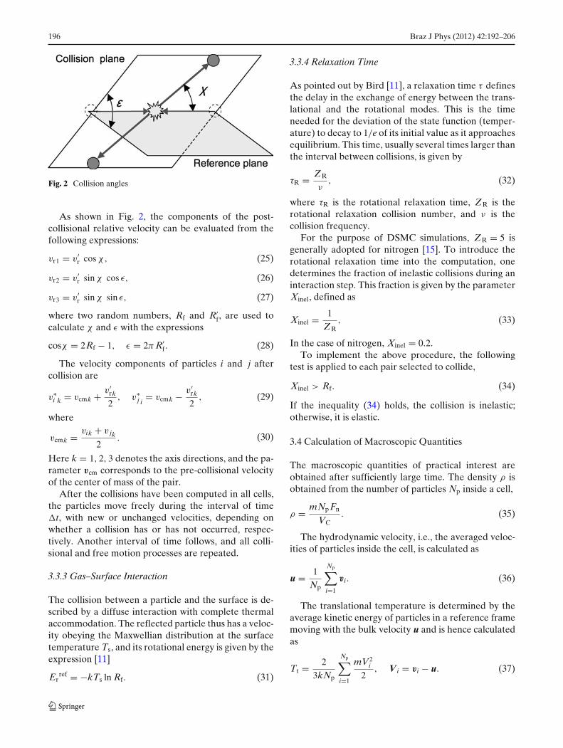
Fig. 2 Collision angles
As shown in Fig. 2, the components of the post-collisional relative velocity can be evaluated from thefollowing expressions:
vr1 = v′r cos χ, (25)
vr2 = v′r sin χ cos ε, (26)
vr3 = v′r sin χ sin ε, (27)
where two random numbers, Rf and R′f, are used to
calculate χ and ε with the expressions
cosχ = 2Rf − 1, ε = 2π R′f. (28)
The velocity components of particles i and j aftercollision are
v∗i k = vcmk + v′
rk
2, v∗
j i= vcmk − v′
rk
2, (29)
where
vcmk = vik + v jk
2. (30)
Here k = 1, 2, 3 denotes the axis directions, and the pa-rameter vcm corresponds to the pre-collisional velocityof the center of mass of the pair.
After the collisions have been computed in all cells,the particles move freely during the interval of time�t, with new or unchanged velocities, depending onwhether a collision has or has not occurred, respec-tively. Another interval of time follows, and all colli-sional and free motion processes are repeated.
3.3.3 Gas–Surface Interaction
The collision between a particle and the surface is de-scribed by a diffuse interaction with complete thermalaccommodation. The reflected particle thus has a veloc-ity obeying the Maxwellian distribution at the surfacetemperature Ts, and its rotational energy is given by theexpression [11]
Erref = −kTs ln Rf. (31)
3.3.4 Relaxation Time
As pointed out by Bird [11], a relaxation time τ definesthe delay in the exchange of energy between the trans-lational and the rotational modes. This is the timeneeded for the deviation of the state function (temper-ature) to decay to 1/e of its initial value as it approachesequilibrium. This time, usually several times larger thanthe interval between collisions, is given by
τR = ZR
ν, (32)
where τR is the rotational relaxation time, ZR is therotational relaxation collision number, and ν is thecollision frequency.
For the purpose of DSMC simulations, ZR = 5 isgenerally adopted for nitrogen [15]. To introduce therotational relaxation time into the computation, onedetermines the fraction of inelastic collisions during aninteraction step. This fraction is given by the parameterXinel, defined as
Xinel = 1ZR
, (33)
In the case of nitrogen, Xinel = 0.2.To implement the above procedure, the following
test is applied to each pair selected to collide,
Xinel > Rf. (34)
If the inequality (34) holds, the collision is inelastic;otherwise, it is elastic.
3.4 Calculation of Macroscopic Quantities
The macroscopic quantities of practical interest areobtained after sufficiently large time. The density ρ isobtained from the number of particles Np inside a cell,
ρ = mNp Fn
VC. (35)
The hydrodynamic velocity, i.e., the averaged veloc-ities of particles inside the cell, is calculated as
u = 1Np
Np∑i=1
vi. (36)
The translational temperature is determined by theaverage kinetic energy of particles in a reference framemoving with the bulk velocity u and is hence calculatedas
Tt = 23kNp
Np∑i=1
mV2i
2, V i = vi − u. (37)
Braz J Phys (2012) 42:192–206 197
The rotational temperature, directly related to therotational energy of the particles, is obtained from theequality
Tr = 1kNp
Np∑i=1
Eri. (38)
For monatomic gases, the thermodynamic tempera-ture, or simply the temperature, is evaluated as
T = Tt, (39)
For diatomic gases, one defines an overall kinetictemperature Tov, given by the expression
Tov = 3Tt + 2Tr
5. (40)
In thermodynamic equilibrium, Tt = Tr. We hencehave that
T = Tov. (41)
The satellite surface is divided in area segments As,and the net energy that arrives at an area segmentduring an interval of time t is given by the equality
enet = 1Ast
×Ns∑
i=1
[m(vref
i )2
2− m(vinc
i )2
2+ Er
refi − Er
inci
], (42)
where vinci is the velocity of particle incident on the
surface, vrefi is the velocity of particle reflected from
the surface, Erinci is the rotational energy of particle
incident on the surface, Errefi is the rotational energy
of particle reflected from the surface, and t is the timefor statistical accumulation.
Since the only mechanism of energy transfer on thesatellite surface is due to the molecular collisions, theenergy flow is given by the expression
qn = enet. (43)
The coefficients Ch, Cp, and Cf are also obtained fromthe number of particles Ns colliding with each segmentduring a time interval t.
For the energy transfer coefficient, defined by (10),we have that
Ch = 1pdU∞
1Ast
×Ns∑
i=1
[m(vref
i )2
2− m(vinc
i )2
2+ Er
refi − Er
inci
]. (44)
For the pressure coefficient, defined by (11), we maywrite that
Cp = 1pd
[1
Ast
Ns∑i=1
m(vrefni − vinc
ni ) − p∞
], (45)
where vincni (vref
ni ) is the normal component of the velocityof a particles incident on (reflected from) the surface.
For the friction coefficient, defined by (12), we havethat
Cf = 1pd
1Ast
Ns∑i=1
m(vrefti − vinc
ti ), (46)
where vincti (vref
ti ) is the tangential component of thevelocity of a particle incident on (reflected from) thesurface.
For the drag coefficient, defined by the expression(7), we have the following relation:
Cd = 1pdπ R2
s
1t
Ns∑i=1
m(vincxi − vref
xi ), (47)
where vincxi (vref
xi ) is the horizontal component, in the x di-rection, of the velocity of particle incident on (reflectedfrom) the surface.
3.5 Grid
We lay the cells on a multilevel, regular grid. Thisarrangement allows finer discretization where the flowproperties have larger gradients and in the neighbor-hood of the satellite surface, to minimize the effect ofrectangular grid irregularities.
The region under study has cylindrical symmetry.The radius of the flowfield is three times larger thanthe radius of the satellite base, and other lengths aredefined as shown in Fig. 3. The (linear) dimensionof the cells in the neighborhood of the satellite ishalf the dimension of those far away. Corrections are
Fig. 3 Grid of cells used in the DSMC code
198 Braz J Phys (2012) 42:192–206
introduced to account for the smaller volumes of thecells on the surface of the satellite.
3.6 Other Computational Parameters
Model particles are substituted for the much morenumerous real particles. The space is discretized in cellsof finite size �r, and the time is discretized in intervalsof size �t. The accuracy of the calculation is expected toimprove as the number of model particles approachesthe number of real particles and as �r and �t shrinkin comparison with the mean free path and the meantime between molecular collisions, respectively. Con-siderations of computational cost imposing constraintson the three parameters, we choose an average numberof 2 × 10⁶ model particles, larger cells of size R/12, asindicated in Fig. 3, and time increments �t given by theequality
�t = 0.01R(
m2kT∞
)1/2
. (48)
Comparison with tests in which the number of par-ticles was doubled, while the cell size and the timeincrement were halved, has shown that the above pa-rameters limit the numeric uncertainty to about 1% forthe drag coefficient and to between 1% and 10% forthe other quantities. The computational time necessaryto achieve the desired results varied from 2 to 3 days toa month, depending on the Reynolds number.
4 Numerical Results
4.1 General Remarks
The calculations of the flow around the satellite werecarried out for the Reynolds numbers ranging fromRe = 0.1 to Re = 10,000 and for two Mach numbersMa = 10 to Ma = 20. According to the expression (6),the rarefaction parameter varies from δ ≈ 0.01 (freemolecule regime) to δ ≈ 600 (hydrodynamic regime).These values will represent the typical magnitudesof the Reynolds and Mach numbers during an at-mospheric reentry.
Since the satellite is highly heated during a reentry,it is interesting to evaluate the influence of the temper-ature of satellite surface Ts on the aerothermodynamiccharacteristics of the satellite. To do this, two values ofthe temperature ratio Ts/T∞ were considered: 1 and10. The first ratio corresponds to a satellite surface atthe unperturbed flow temperature, T∞, i.e., the satelliteis “cold.” The second value, Ts/T∞ = 10, correspondsto a satellite surface at a considerably higher temper-
Table 1 Parameters for monatomic and diatomic gases
ature than the unperturbed flow, i.e., the satellite is“hot.” In reality, the surface temperature should varywithin the range defined by these two extremes, andthe two calculations should reveal the magnitude ofthe influence of the satellite surface temperature on itsaerothermodynamic characteristics.
To evaluate the difference between the monatomicand diatomic gases, both cases were simulated, threeparameters being varied as shown in Table 1, whereγ is the ratio between specific heats of the gas; ω isthe exponent of the viscosity law, defined by (18); andXinel is the parameter defining the fraction of inelasticcollisions, as has been explained in Section 3.3.4.
4.2 Drag Coefficient
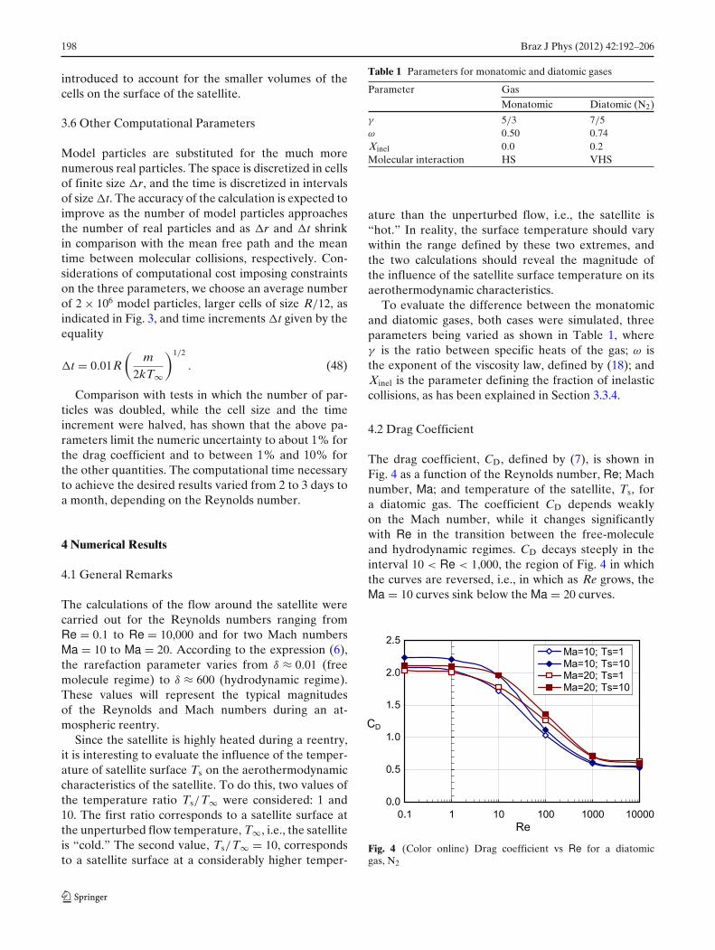
The drag coefficient, CD, defined by (7), is shown inFig. 4 as a function of the Reynolds number, Re; Machnumber, Ma; and temperature of the satellite, Ts, fora diatomic gas. The coefficient CD depends weaklyon the Mach number, while it changes significantlywith Re in the transition between the free-moleculeand hydrodynamic regimes. CD decays steeply in theinterval 10 < Re < 1,000, the region of Fig. 4 in whichthe curves are reversed, i.e., in which as Re grows, theMa = 10 curves sink below the Ma = 20 curves.
Fig. 4 (Color online) Drag coefficient vs Re for a diatomicgas, N2
Braz J Phys (2012) 42:192–206 199
Comparison between the results for the “cold”(Ts/T∞ = 1) and the “hot” (Ts/T∞ = 10) satellitesshows that the drag coefficient CD is most sensitiveto the satellite temperature near the free moleculesregime, i.e., for Re = 0.1, and for the smaller Machnumber in this work, Ma = 10. The change is then closeto 9%. The Mach number being larger than 10 underthe conditions of satellite reentry, we conclude that thesatellite temperature has little influence on the dragcoefficient.
As a first approximation, neglecting the small effectsof the surface temperature (Ts) and of the Machnumber (Ma) on the drag coefficient, we obtained anaccurate fit to the data in Fig. 4 with the followingexpression:
CD = 1.5721 + 0.02568 e(2.031 log Re)
+ 0.5493. (49)
To evaluate the influence of the monatomic gas anddiatomic gas hypotheses in the flow simulation, numer-ical data for CD are shown in Table 2. At Ma = 10, thedrag coefficient of the diatomic gas becomes somewhatsmaller than the coefficient of the monatomic gas inthe transition region, with a slight inversion after Re ≈1,000. These changes are very close to the accuracy ofthe calculation. At Ma = 20, the difference becomesmore noticeable, albeit small. For Re > 1,000, the dragcoefficient of the diatomic gas is 2–3% smaller than thatof the monatomic gas.
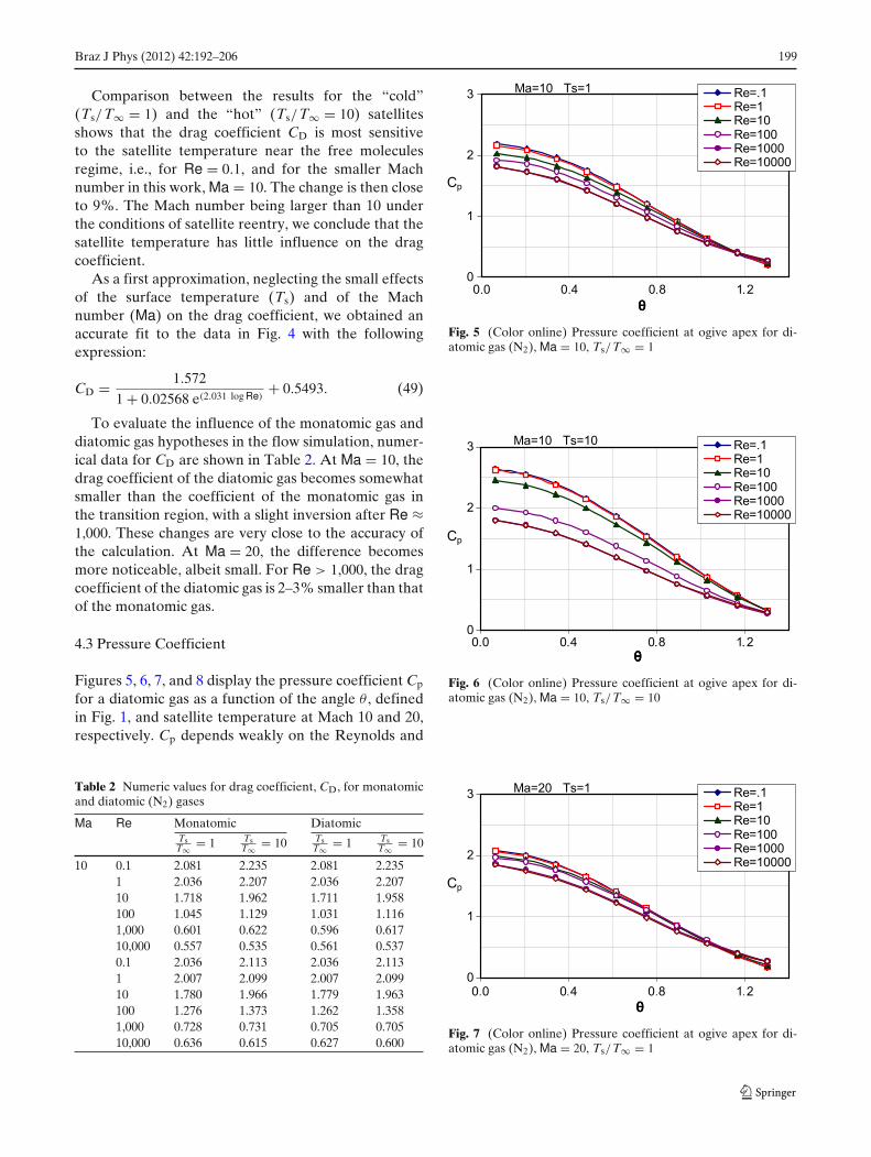
4.3 Pressure Coefficient
Figures 5, 6, 7, and 8 display the pressure coefficient Cp
for a diatomic gas as a function of the angle θ , definedin Fig. 1, and satellite temperature at Mach 10 and 20,respectively. Cp depends weakly on the Reynolds and
Table 2 Numeric values for drag coefficient, CD, for monatomicand diatomic (N2) gases
Fig. 5 (Color online) Pressure coefficient at ogive apex for di-atomic gas (N2), Ma = 10, Ts/T∞ = 1
Fig. 6 (Color online) Pressure coefficient at ogive apex for di-atomic gas (N2), Ma = 10, Ts/T∞ = 10
Fig. 7 (Color online) Pressure coefficient at ogive apex for di-atomic gas (N2), Ma = 20, Ts/T∞ = 1
200 Braz J Phys (2012) 42:192–206
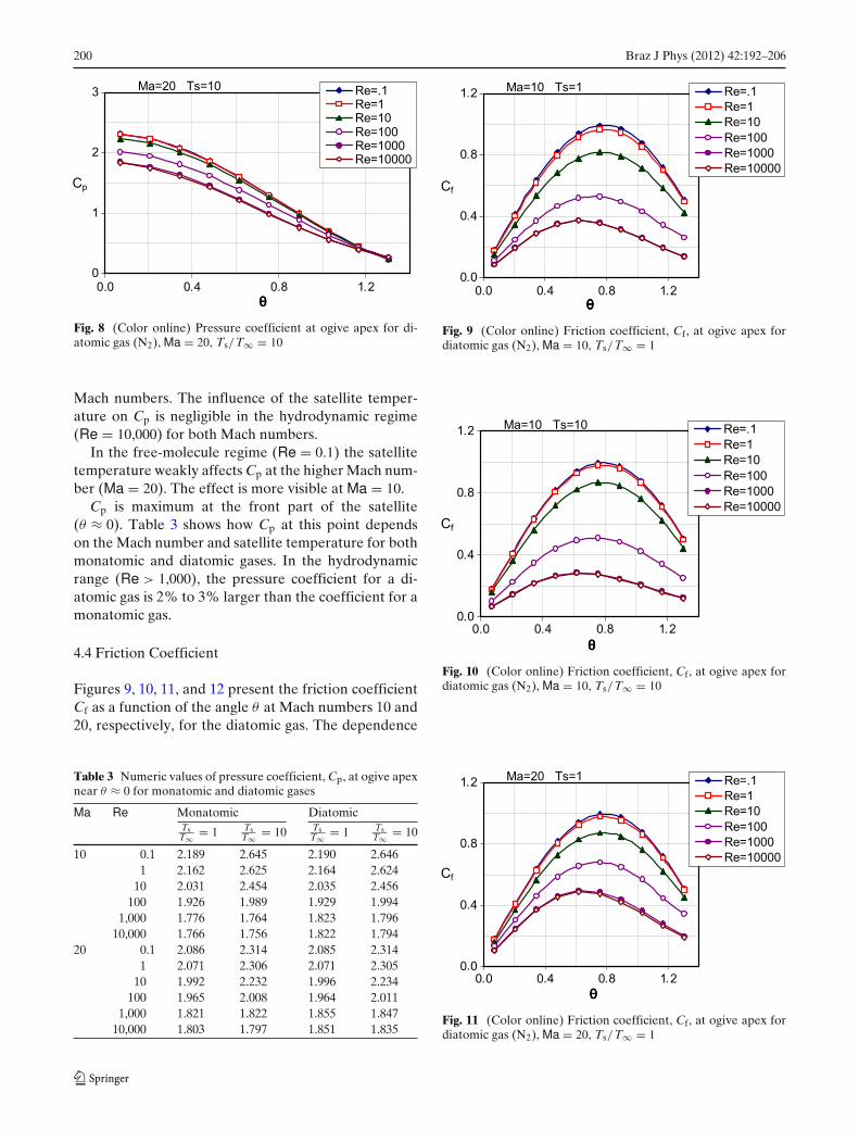
Fig. 8 (Color online) Pressure coefficient at ogive apex for di-atomic gas (N2), Ma = 20, Ts/T∞ = 10
Mach numbers. The influence of the satellite temper-ature on Cp is negligible in the hydrodynamic regime(Re = 10,000) for both Mach numbers.
In the free-molecule regime (Re = 0.1) the satellitetemperature weakly affects Cp at the higher Mach num-ber (Ma = 20). The effect is more visible at Ma = 10.
Cp is maximum at the front part of the satellite(θ ≈ 0). Table 3 shows how Cp at this point dependson the Mach number and satellite temperature for bothmonatomic and diatomic gases. In the hydrodynamicrange (Re > 1,000), the pressure coefficient for a di-atomic gas is 2% to 3% larger than the coefficient for amonatomic gas.
4.4 Friction Coefficient
Figures 9, 10, 11, and 12 present the friction coefficientCf as a function of the angle θ at Mach numbers 10 and20, respectively, for the diatomic gas. The dependence
Table 3 Numeric values of pressure coefficient, Cp, at ogive apexnear θ ≈ 0 for monatomic and diatomic gases
Fig. 9 (Color online) Friction coefficient, Cf, at ogive apex fordiatomic gas (N2), Ma = 10, Ts/T∞ = 1
Fig. 10 (Color online) Friction coefficient, Cf, at ogive apex fordiatomic gas (N2), Ma = 10, Ts/T∞ = 10
Fig. 11 (Color online) Friction coefficient, Cf, at ogive apex fordiatomic gas (N2), Ma = 20, Ts/T∞ = 1
Braz J Phys (2012) 42:192–206 201
Fig. 12 (Color online) Friction coefficient, Cf, at ogive apex fordiatomic gas (N2), Ma = 20, Ts/T∞ = 10
on the Reynolds number Re highlights the effects ofrarefaction. The steep rise in Cf as Re indicates that thefriction coefficient is sensitive to gas rarefaction.
For high Re, the friction coefficient is also sensitiveto changes in the Mach number. For Re = 10,000, rela-tive to Cf at Ma = 10, the friction coefficient is nearly30% higher for the “cold” satellite and 45% higherfor the “hot” satellite. By contrast, at low Reynoldnumbers, the coefficient is practically independent ofthe Mach number.
At fixed Ma, in the free-molecule regime (Re =0.1), the friction coefficient is likewise insensitive tochanges in the satellite temperature. In the hydrody-namic regime (Re ≥ 1,000), the coefficient does dependon the satellite temperature: The maximum Cf for the“hot” satellite is 15% to 20% larger than the maximumfor the “cold” one.
The maximum friction coefficient is in the vicinity ofθ = π/4. Table 4 lists values of Cf at this point for vari-
Table 4 Numerical values of friction coefficient, Cf, at ogive apexnear θ = π/4 for monatomic and diatomic (N2) gases
Fig. 13 (Color online) Energy transfer coefficient, Ch, at ogiveapex for diatomic gas (N2), Ma = 10, Ts/T∞ = 1
ous Reynolds and Mach numbers, for both monatomicand diatomic gases. Again, the dependences on theMach number and satellite temperature are weak in thefree-molecule regime and stronger the hydrodynamicregime. While the Cf coefficient tends to be a littlelarger for the diatomic gas, the differences between theresults for the monatomic and diatomic gas becomenoticeable only when the “cold” satellite is in the hy-drodynamic regime at the higher Mach number.
4.5 Energy Transfer Coefficient
Figures 13, 14, 15, and 16 show that the energy transfercoefficient Ch as a function of θ is for a diatomic gasin for Ts/T∞ = 1 (“cold” satellite) and Ts/T∞ = 10(“hot” satellite). Ch is very sensitive to changes in theReynolds number (Re): It grows with rarefaction, i.e.,as Re decreases. The dependence on the Mach number
Fig. 14 (Color online) Energy transfer coefficient, Ch, at ogiveapex for diatomic gas (N2), Ma = 10, Ts/T∞ = 10
202 Braz J Phys (2012) 42:192–206
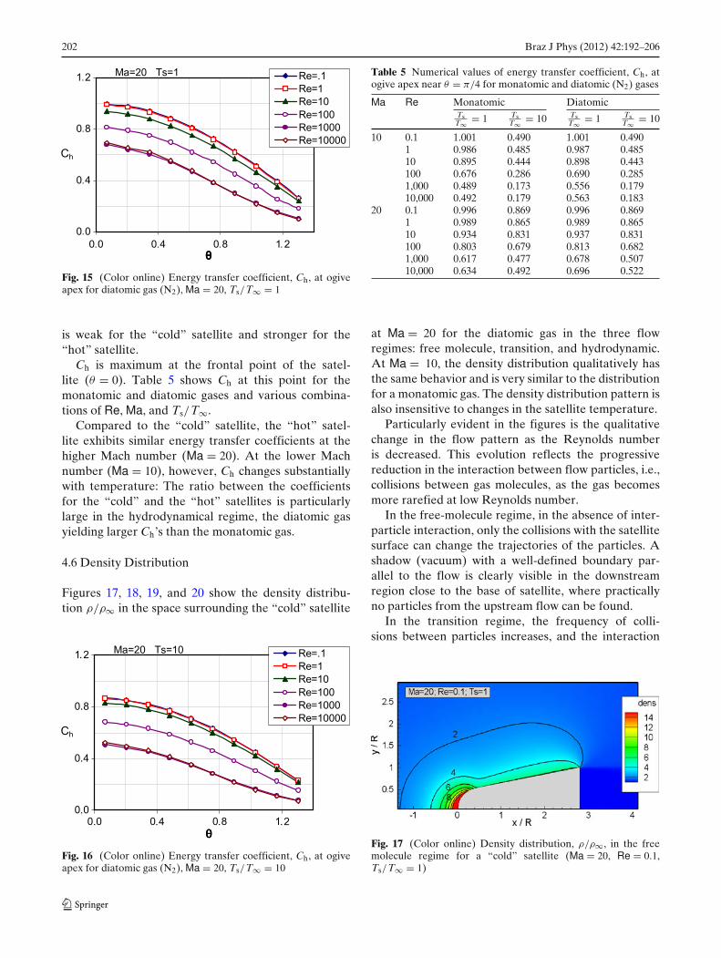
Fig. 15 (Color online) Energy transfer coefficient, Ch, at ogiveapex for diatomic gas (N2), Ma = 20, Ts/T∞ = 1
is weak for the “cold” satellite and stronger for the“hot” satellite.
Ch is maximum at the frontal point of the satel-lite (θ = 0). Table 5 shows Ch at this point for themonatomic and diatomic gases and various combina-tions of Re, Ma, and Ts/T∞.
Compared to the “cold” satellite, the “hot” satel-lite exhibits similar energy transfer coefficients at thehigher Mach number (Ma = 20). At the lower Machnumber (Ma = 10), however, Ch changes substantiallywith temperature: The ratio between the coefficientsfor the “cold” and the “hot” satellites is particularlylarge in the hydrodynamical regime, the diatomic gasyielding larger Ch’s than the monatomic gas.
4.6 Density Distribution
Figures 17, 18, 19, and 20 show the density distribu-tion ρ/ρ∞ in the space surrounding the “cold” satellite
Fig. 16 (Color online) Energy transfer coefficient, Ch, at ogiveapex for diatomic gas (N2), Ma = 20, Ts/T∞ = 10
Table 5 Numerical values of energy transfer coefficient, Ch, atogive apex near θ = π/4 for monatomic and diatomic (N2) gases
at Ma = 20 for the diatomic gas in the three flowregimes: free molecule, transition, and hydrodynamic.At Ma = 10, the density distribution qualitatively hasthe same behavior and is very similar to the distributionfor a monatomic gas. The density distribution pattern isalso insensitive to changes in the satellite temperature.
Particularly evident in the figures is the qualitativechange in the flow pattern as the Reynolds numberis decreased. This evolution reflects the progressivereduction in the interaction between flow particles, i.e.,collisions between gas molecules, as the gas becomesmore rarefied at low Reynolds number.
In the free-molecule regime, in the absence of inter-particle interaction, only the collisions with the satellitesurface can change the trajectories of the particles. Ashadow (vacuum) with a well-defined boundary par-allel to the flow is clearly visible in the downstreamregion close to the base of satellite, where practicallyno particles from the upstream flow can be found.
In the transition regime, the frequency of colli-sions between particles increases, and the interaction
Fig. 17 (Color online) Density distribution, ρ/ρ∞, in the freemolecule regime for a “cold” satellite (Ma = 20, Re = 0.1,Ts/T∞ = 1)
Braz J Phys (2012) 42:192–206 203
Fig. 18 (Color online) Density distribution, ρ/ρ∞, in the transi-tion regime for a “cold” satellite (Ma = 20, Re = 10, Ts/T∞ = 1)
between the oncoming flow and reflected particlesbecomes noticeable as the region of inhomogeneousdensity narrows and acquires a more distinct boundary.Finally, in the hydrodynamical regime, the region ofinhomogeneous density becomes well delimited by abow (detached) shock wave.
4.7 Temperature Distribution
Figures 21, 22, 23, and 24 show the temperature distrib-ution T/T∞ in the space surrounding the “cold” satel-lite for Ma = 20 and a diatomic gas in the three flowregimes: free molecule, transition, and hydrodynamic.The temperature distribution at Ma = 10 is qualita-tively the same, and practically no differences are foundwhen a monatomic gas is substituted for the diatomicgas. Likewise, the temperature distributions around a“hot” satellite are very similar.
The temperature distribution clearly shows the qual-itative difference between the three flow regimes.In the hydrodynamic regime (Re = 10,000), the bowshock in front of the satellite is easily recognized;with increasing rarefaction (Re = 100 and 10–transitionregime) the shock moves away from the satellite and
Fig. 19 (Color online) Density distribution, ρ/ρ∞, in thetransition regime for a “cold” satellite (Ma = 20, Re = 100,Ts/T∞ = 1)
Fig. 20 (Color online) Density distribution, ρ/ρ∞, in the hy-drodynamic regime for a “cold” satellite (Ma = 20, Re = 10,000,Ts/T∞ = 1)
Fig. 21 (Color online) Temperature distribution, T/T∞, in thefree molecule regime for a “cold” satellite (Ma = 20, Re = 0.1,Ts/T∞ = 1)
Fig. 22 (Color online) Temperature distribution, T/T∞, inthe transition regime for a “cold” satellite (Ma = 20, Re = 10,Ts/T∞ = 1)
Fig. 23 (Color online) Temperature distribution, T/T∞, in thetransition regime for a “cold” satellite (Ma = 20, Re = 100,Ts/T∞ = 1)
204 Braz J Phys (2012) 42:192–206
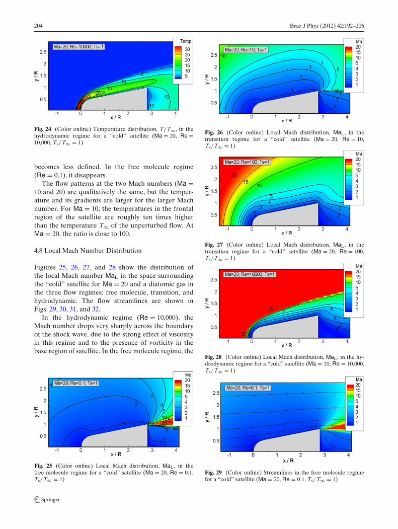
Fig. 24 (Color online) Temperature distribution, T/T∞, in thehydrodynamic regime for a “cold” satellite (Ma = 20, Re =10,000, Ts/T∞ = 1)
becomes less defined. In the free molecule regime(Re = 0.1), it disappears.
The flow patterns at the two Mach numbers (Ma =10 and 20) are qualitatively the same, but the temper-ature and its gradients are larger for the larger Machnumber. For Ma = 10, the temperatures in the frontalregion of the satellite are roughly ten times higherthan the temperature T∞ of the unperturbed flow. AtMa = 20, the ratio is close to 100.
4.8 Local Mach Number Distribution
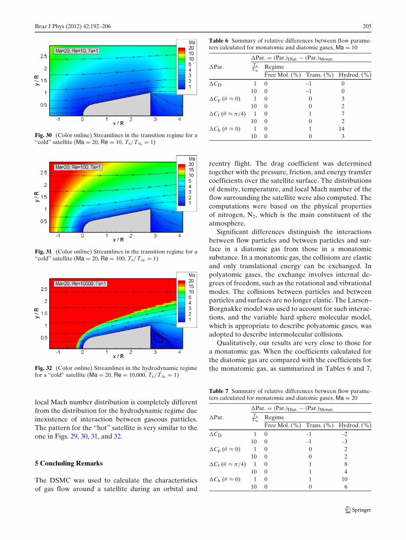
Figures 25, 26, 27, and 28 show the distribution ofthe local Mach number MaL in the space surroundingthe “cold” satellite for Ma = 20 and a diatomic gas inthe three flow regimes: free molecule, transition, andhydrodynamic. The flow streamlines are shown inFigs. 29, 30, 31, and 32.
In the hydrodynamic regime (Re = 10,000), theMach number drops very sharply across the boundaryof the shock wave, due to the strong effect of viscosityin this regime and to the presence of vorticity in thebase region of satellite. In the free molecule regime, the
Fig. 25 (Color online) Local Mach distribution, MaL, in thefree molecule regime for a “cold” satellite (Ma = 20, Re = 0.1,Ts/T∞ = 1)
Fig. 26 (Color online) Local Mach distribution, MaL, in thetransition regime for a “cold” satellite (Ma = 20, Re = 10,Ts/T∞ = 1)
Fig. 27 (Color online) Local Mach distribution, MaL, in thetransition regime for a “cold” satellite (Ma = 20, Re = 100,Ts/T∞ = 1)
Fig. 28 (Color online) Local Mach distribution, MaL, in the hy-drodynamic regime for a “cold” satellite (Ma = 20, Re = 10,000,Ts/T∞ = 1)
Fig. 29 (Color online) Streamlines in the free molecule regimefor a “cold” satellite (Ma = 20, Re = 0.1, Ts/T∞ = 1)
Braz J Phys (2012) 42:192–206 205
Fig. 30 (Color online) Streamlines in the transition regime for a“cold” satellite (Ma = 20, Re = 10, Ts/T∞ = 1)
Fig. 31 (Color online) Streamlines in the transition regime for a“cold” satellite (Ma = 20, Re = 100, Ts/T∞ = 1)
Fig. 32 (Color online) Streamlines in the hydrodynamic regimefor a “cold” satellite (Ma = 20, Re = 10,000, Ts/T∞ = 1)
local Mach number distribution is completely differentfrom the distribution for the hydrodynamic regime dueinexistence of interaction between gaseous particles.The pattern for the “hot” satellite is very similar to theone in Figs. 29, 30, 31, and 32.
5 Concluding Remarks
The DSMC was used to calculate the characteristicsof gas flow around a satellite during an orbital and
Table 6 Summary of relative differences between flow parame-ters calculated for monatomic and diatomic gases, Ma = 10
�Par. = (Par.)Diat. − (Par.)Monat.
�Par. TsT∞ Regime
Free Mol. (%) Trans. (%) Hydrod. (%)
�CD 1 0 –1 010 0 –1 0
�Cp (θ ≈ 0) 1 0 0 310 0 0 2
�Cf (θ ≈ π/4) 1 0 1 710 0 0 2
�Ch (θ ≈ 0) 1 0 1 1410 0 0 3
reentry flight. The drag coefficient was determinedtogether with the pressure, friction, and energy transfercoefficients over the satellite surface. The distributionsof density, temperature, and local Mach number of theflow surrounding the satellite were also computed. Thecomputations were based on the physical propertiesof nitrogen, N2, which is the main constituent of theatmosphere.
Significant differences distinguish the interactionsbetween flow particles and between particles and sur-face in a diatomic gas from those in a monatomicsubstance. In a monatomic gas, the collisions are elasticand only translational energy can be exchanged. Inpolyatomic gases, the exchange involves internal de-grees of freedom, such as the rotational and vibrationalmodes. The collisions between particles and betweenparticles and surfaces are no longer elastic. The Larsen–Borgnakke model was used to account for such interac-tions, and the variable hard sphere molecular model,which is appropriate to describe polyatomic gases, wasadopted to describe intermolecular collisions.
Qualitatively, our results are very close to those fora monatomic gas. When the coefficients calculated forthe diatomic gas are compared with the coefficients forthe monatomic gas, as summarized in Tables 6 and 7,
Table 7 Summary of relative differences between flow parame-ters calculated for monatomic and diatomic gases, Ma = 20
�Par. = (Par.)Diat. − (Par.)Monat.
�Par. TsT∞ Regime
Free Mol. (%) Trans. (%) Hydrod. (%)
�CD 1 0 –1 –210 0 –1 –3
�Cp (θ ≈ 0) 1 0 0 210 0 0 2
�Cf (θ ≈ π/4) 1 0 1 810 0 1 4
�Ch (θ ≈ 0) 1 0 1 1010 0 0 6
206 Braz J Phys (2012) 42:192–206
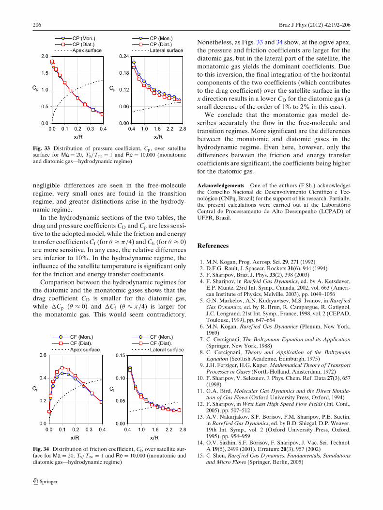
Fig. 33 Distribution of pressure coefficient, Cp, over satellitesurface for Ma = 20, Ts/T∞ = 1 and Re = 10,000 (monatomicand diatomic gas—hydrodynamic regime)
negligible differences are seen in the free-moleculeregime, very small ones are found in the transitionregime, and greater distinctions arise in the hydrody-namic regime.
In the hydrodynamic sections of the two tables, thedrag and pressure coefficients CD and Cp are less sensi-tive to the adopted model, while the friction and energytransfer coefficients Cf (for θ ≈ π/4) and Ch (for θ ≈ 0)are more sensitive. In any case, the relative differencesare inferior to 10%. In the hydrodynamic regime, theinfluence of the satellite temperature is significant onlyfor the friction and energy transfer coefficients.
Comparison between the hydrodynamic regimes forthe diatomic and the monatomic gases shows that thedrag coefficient CD is smaller for the diatomic gas,while �Cp (θ ≈ 0) and �Cf (θ ≈ π/4) is larger forthe monatomic gas. This would seem contradictory.
Fig. 34 Distribution of friction coefficient, Cf, over satellite sur-face for Ma = 20, Ts/T∞ = 1 and Re = 10,000 (monatomic anddiatomic gas—hydrodynamic regime)
Nonetheless, as Figs. 33 and 34 show, at the ogive apex,the pressure and friction coefficients are larger for thediatomic gas, but in the lateral part of the satellite, themonatomic gas yields the dominant coefficients. Dueto this inversion, the final integration of the horizontalcomponents of the two coefficients (which contributesto the drag coefficient) over the satellite surface in thex direction results in a lower CD for the diatomic gas (asmall decrease of the order of 1% to 2% in this case).
We conclude that the monatomic gas model de-scribes accurately the flow in the free-molecule andtransition regimes. More significant are the differencesbetween the monatomic and diatomic gases in thehydrodynamic regime. Even here, however, only thedifferences between the friction and energy transfercoefficients are significant, the coefficients being higherfor the diatomic gas.
Acknowledgements One of the authors (F.Sh.) acknowledgesthe Conselho Nacional de Desenvolvimento Científico e Tec-nológico (CNPq, Brazil) for the support of his research. Partially,the present calculations were carried out at the LaboratórioCentral de Processamento de Alto Desempenho (LCPAD) ofUFPR, Brazil.
References
1. M.N. Kogan, Prog. Aerosp. Sci. 29, 271 (1992)2. D.F.G. Rault, J. Spacecr. Rockets 31(6), 944 (1994)3. F. Sharipov, Braz. J. Phys. 33(2), 398 (2003)4. F. Sharipov, in Rarfeid Gas Dynamics, ed. by A. Ketsdever,
E.P. Muntz. 23rd Int. Symp., Canada, 2002, vol. 663 (Ameri-can Institute of Physics, Melville, 2003), pp. 1049–1056
5. G.N. Markelov, A.N. Kudryavtsev, M.S. Ivanov, in Raref iedGas Dynamics, ed. by R. Brun, R. Campargue, R. Gatignol,J.C. Lengrand. 21st Int. Symp., France, 1998, vol. 2 (CEPAD,Toulouse, 1999), pp. 647–654
6. M.N. Kogan, Raref ied Gas Dynamics (Plenum, New York,1969)
7. C. Cercignani, The Boltzmann Equation and its Application(Springer, New York, 1988)
8. C. Cercignani, Theory and Application of the BoltzmannEquation (Scottish Academic, Edinburgh, 1975)
9. J.H. Ferziger, H.G. Kaper, Mathematical Theory of TransportProcesses in Gases (North-Holland, Amsterdam, 1972)
10. F. Sharipov, V. Seleznev, J. Phys. Chem. Ref. Data 27(3), 657(1998)
11. G.A. Bird, Molecular Gas Dynamics and the Direct Simula-tion of Gas Flows (Oxford University Press, Oxford, 1994)
12. F. Sharipov, in West East High Speed Flow Fields (Int. Conf.,2005), pp. 507–512
13. A.V. Nakarjakov, S.F. Borisov, F.M. Sharipov, P.E. Suetin,in Raref ied Gas Dynamics, ed. by B.D. Shizgal, D.P. Weaver.19th Int. Symp., vol. 2 (Oxford University Press, Oxford,1995), pp. 954–959
14. O.V. Sazhin, S.F. Borisov, F. Sharipov, J. Vac. Sci. Technol.A 19(5), 2499 (2001). Erratum: 20(3), 957 (2002)
15. C. Shen, Raref ied Gas Dynamics. Fundamentals, Simulationsand Micro Flows (Springer, Berlin, 2005)