A Portfolio Optimization Model with Regime-Switching Risk Factors for Sector Exchange Traded Funds * Ying Ma † Leonard MacLean ‡ Kuan Xu § Yonggan Zhao ¶ March 6, 2011 Keywords: sector exchange traded fund, factor risk neutral, Markov regime switch- ing, factor risk, portfolio optimization * Yonggan Zhao acknowledges financial support from the Natural Sciences and Engineering Re- search Council of Canada, the Social Sciences and Humanities Research Council of Canada, and the Canada Research Chairs Program. Leonard MacLean acknowledges financial support from the Nat- ural Sciences and Engineering Research Council of Canada and The Herbert Lamb Trust. Kuan Xu acknowledges financial support from Dalhousie University and Renmin University. † Department of Economics, Dalhousie University ‡ School of Business Administration, Dalhousie University § Department of Economics, Dalhousie University ¶ Corresponding author, School of Business Administration, Dalhousie University, Halifax, Nova Scotia, Canada, B3H 3J5, Phone: (902)494-6972, Email: [email protected]1
Transcript
A Portfolio Optimization Model withRegime-Switching Risk Factors for Sector
∗Yonggan Zhao acknowledges financial support from the Natural Sciences and Engineering Re-search Council of Canada, the Social Sciences and Humanities Research Council of Canada, and theCanada Research Chairs Program. Leonard MacLean acknowledges financial support from the Nat-ural Sciences and Engineering Research Council of Canada and The Herbert Lamb Trust. Kuan Xuacknowledges financial support from Dalhousie University and Renmin University.†Department of Economics, Dalhousie University‡School of Business Administration, Dalhousie University§Department of Economics, Dalhousie University¶Corresponding author, School of Business Administration, Dalhousie University, Halifax, Nova
A Portfolio Optimization Model withRegime-Switching Risk Factors for Sector Exchange
Traded Funds
Abstract
This paper develops a portfolio optimization model with a market neutral strat-
egy under a Markov regime-switching framework. The selected investment in-
struments consist of the nine sector exchange traded funds (ETFs) that represent
the U.S. stock market. The Bayesian information criterion is used to determine
the optimal number of regimes. The investment objective is to dynamically maxi-
mize the portfolio alpha (excess return over the T-Bill) subject to neutralization of
the portfolio sensitivities to the selected risk factors. The portfolio risk exposures
are shown to change with various style and macro factors over time. The maxi-
mization problem in this context can be established as a regime-dependent linear
programming problem. The optimal portfolio constructed as such is expected to
outperform a naive benchmark strategy, which equally weights the ETFs. We
evaluate the in-sample and out-of-sample performance of the regime-dependent
market neutral strategy against the equally weighted strategy. We find that the
former generally outperforms the latter.
2
1 Introduction
The goal of investment is to maximize the expected return of an asset portfolio withlimited risk exposure. This investment objective is usually constrained with thechanging economic conditions and the state-dependent risk factors. Dynamic assetallocation is a process of selecting investment instruments and constructing optimalportfolios over time.
The performance of any investment portfolio depends on the accuracy of forecastof asset returns and relevant risk factors. Chen, Ross and Roll (1986) studied anasset pricing model using macro economic risk factors such as the growth rate of in-dustrial production (IP), unexpected inflation (UI), change of expected inflation (DEI),yield spread (YS) and credit spread (CS). They found that each factor is significantin predicting stock returns. Fama and French (1993) investigated an asset pricingmodel using three style factors: the excess market portfolio return over the risk freeasset (MKT), difference of returns on the small and large stock portfolios (SML), anddifference of returns on high and low book-to-market ratio portfolio returns (HML).However, neither Chen, Ross, and Roll (1986) nor Fama and French (1993) addressedthe regime-dependent nature of the sensitivities of asset returns to the risk factors.In this paper, we develop an investment model incorporating market regimes whichcharacterize different patterns of asset returns in the unobservable economic situa-tions, such as bear and bull markets.
Investment securities may exhibit different risk levels in different economic situ-ations and, therefore, different risk premiums. However, there is no clear determina-tion as to which economic regime we are in by directly observing the market data. Thekey idea for a regime switching model is to resolve the issue of unobserved economicregimes over time. Previous research has indicated that a probability distributionwith a structural Markov chain is sufficient to describe the dynamics of the economicregimes. Hamilton (1989) successfully applied a two-regime hidden Markov modelto the U.S. GDP data and characterized the changing pattern of the US economy.Cai (1994), Hamilton (1998), and Gray (1996) used variations of the Markov regime-switching model to describe the time series behavior of U.S. short-term interest rates.Bekaert and Hodrick (1993) documented regime shifts in major foreign exchangerates. Schwert (1989) considered that asset returns may be associated with eitherhigh or low volatility regimes which switch over time. Whitelaw (2001) constructedan equilibrium model where growth in consumption follows a regime-switching pro-
3
cess. Liu, Xu and Zhao (2011) showed that the regime-switching model is an effectiveway for linking sector ETF returns to style and macro factors in changing marketregimes over time.
With new empirical evidence supporting regime-switching asset pricing models,regime-dependent asset allocation appears to be a flexible and attractive option toinvestors when market regimes can be properly identified. Ang and Bekaert (2002,2004) studied asset allocation models with regime shifts. Guidolin and Timmermann(2007, 2008) provided important economic insights on how investments vary acrossdifferent market regimes. Recently, Jun Tu (2010) provided a Bayesian frameworkfor making portfolio decisions with regime-switching and asset pricing model uncer-tainty. Berdot, Goyeau and Leonard (2006) studied multi-sector portfolio allocationfor active portfolio management and found that portfolio returns are very differentwith four market regimes.
A standard asset pricing model linearly relates the expected returns to market riskfactors. Under a linear asset pricing model, such as the Capital Asset Pricing Model,the asset “alpha” is usually referred to as the temporary deviation of the expectedreturns from the prediction of the pricing model. Portfolio managers usually pursuea market neutral strategy so that the portfolio’s alpha is maximized with neutralizedrisk exposures.1 This investment strategy is often used in the hedge fund indus-try. According to Capocci (2006), approximately 28.3% of the MAR/CISDM (GlobalManagement Account Reports/Center for International Securities and DerivativesMarkets) individual funds in the database are market neutral funds. Edwards andCaglayan (2001) showed that market neutral strategies provide the investor withpositive returns in the market downturns during the period from 1990 to 1998.
In this paper, we propose a stochastic linear programming model to maximize theportfolio “alpha” with limited risk exposure to the selected risk factors. Accordingto Shyu et al. (2006), this feature is also referred to as the zero-beta strategy. Aspointed out by Gastineau, Olma and Zielinski (2007), this market neutral strategy isimplemented by constructing and rebalancing the portfolio that has overall zero betasfor all relevant risk factors and thus the return of the portfolio under such strategy is
1The standard feature of the market neutral strategy is that, while some assets in a portfolio havelong positions, some assets have short positions simultaneously. In this way the impact of marketmovements can be minimized. In a declining market situation, the short positions earn profits byneutralizing the losses made by long positions. By taking long positions on undervalued assets andshort positions on overvalued assets, steady returns can be captured in all directions of market.
4
uncorrelated with the market risk factors.One of the key equity investment trends in recent years is the growing interest
in the exchange traded funds (ETFs). Unlike traditional mutual funds, these instru-ments are exchange-tradable securities like normal stocks. Investing in a sector ETFis an investment strategy which mimics the performance of the corresponding indus-trial sector. In this paper, an optimization problem is set up for finding the optimalinvestment weights in the nine sector ETFs that represent the U.S. stock marketbased on a regime-dependent market neutral strategy. The performance of the port-folio under the regime-dependent market neutral strategy is then compared with thatof the portfolio under a benchmark strategy, which allocates assets equally across thenine U.S. sector ETFs regardless of the future market regime. The empirical resultsdemonstrate that the regime-dependent market neutral strategy generally outper-forms the benchmark strategy.
2 The Asset Pricing Model
In the financial market, there are many broad asset classes (such as equities, bonds,commodities, currencies, and real estate properties). Asset allocation is made amongthese broad asset classes and there are possibly many different strategies. In this re-search, we only consider equity instruments in the form of the nine U.S. sector ETFs.The Sector SPDRs ETFs cover all sectors of the U.S. stock market such as consumerdiscretionary (XLY), consumer staples (XLP), energy (XLE), financials (XLF), health(XLV), industrials (XLI), materials (XLB), technology (XLK), and utilities (XLU). Thesesector ETFs satisfy four selection criteria: (i) the nine sector ETFs well represent themajor sectors of the U.S. stock market; (ii) the nine sector ETFs are offered by onecompany so as to maintain portfolio consistency and eliminate managerial discrep-ancies; (iii) the nine sector ETFs have a long trading history (started December 23,1998); and (iv) the nine sector ETFs are liquid and have a large daily trading volume.The returns on assets are considered for fixed time periods.
2.1 The basic models
The models for asset returns and investment decisions will be formulated in generaland then specialized to ETFs in the application. Let Pti be the trading price of asseti at time t, with Rti = ln(Pti/Pt−1,i) being the return for the ith (i = 1, · · · , I) asset
5
in period t (t = 1, · · · , T ). The term return will henceforth refer to the logarithm ofgross return. Rt is the vector of the asset returns in period t. It is assumed thatthe financial market in each period can be realized as one of N regimes, with thestatistical distribution of asset returns depending on the regime. Furthermore, theregimes are characterized by a set of J risk factors, which represent broad macro andmicro economic indicators. Let Ftj be the value of the jth risk factor (j = 1, · · · , J) inperiod t. Correspondingly, Ft is the vector of risk factors in period t. Asset returns indifferent market regimes are characterized with the common risk factors Ft.
Suppose that the market is in regime st in period t and consider that the assetreturns are defined by the regime-dependent linear factor model
Rt = Ast +BstFt + Γstet, (1)
where et ∼ N(0, I). The model parameters {Ast , Bst ,Γst} depend on the regime st. Thevector A′
st= (α1st , · · · , αIst) contains the state-depend intercepts of the linear factor
model. The matrix
Bst =
β11st . . . β1Jst
... . . . ...βI1st . . . βIJst
defines the sensitivities of asset returns to the common risk factors in state st. Oneimplication of the linear factor model is that the conditional asset returns within aregime, given the factors, are normally distributed with mean vector µst = Ast +BstFt
and covariance matrix Σst = ΓstΓ′st
.The applicability of the linear factor model for predicting returns in a time period
requires estimates of the regime-dependent parameters and forecasts for the valuesof the factors. Assume that there exist N distinct regimes and the dynamics of themarket regimes follow a Markov chain. With the regimes process {st, t = 0, 1, . . .},consider that the regimes are indexed by n and qtn = Pr[st = n], n = 1, . . . , N . There isan initial regime distribution q0 and a transition probability matrix P = {pmn}, wherethe transition probability from regime m to regime n is given by
pmn = Pr(st+1 = n|st = m),∀m,n. (2)
The conditional returns Rn for regime n have a normal density Rn ∝ fn(r). Theunconditional distribution of the asset returns in period t given regime m in period
6
t− 1 is a mixture of normal distributions: f(r) =N∑n=1
pmnfn(r), which is able to capture
distributional characteristics such as heavy tails. In period t, given regimem in periodt− 1, the unconditional expected asset return is
µtm =N∑n=1
µtnpmn,
and the covariance matrix is
Σtm =N∑n=1
[(µtn − µtm)2 + ΓnΓ′n]pmn.
If the regimes are known in each period, then the estimation of model parametersfrom observations on returns and factors is straightforward. However, the regime ineach period is in fact unknown, as are the model parameters for each regime. Theregime must be inferred and the model parameters must be estimated from data.
2.2 The estimation algorithm
An established estimation procedure for identifying regimes and estimating param-eters is the EM algorithm (see Dempster et al. (1977)). The EM algorithm consistsof two steps. The E-step is the estimation of the missing data for regimes and theM-step is the maximization of the likelihood based on the estimated missing data onregimes. The EM algorithm requires the specification of the number of regimes. Thealgorithm is augmented with a third step, called the N-step, for the determinationof the number of regimes based on the Bayesian information criterion developed bySchwarz (1978).
Denote the model parameters as θ = {Ast , Bst ,Γst , q0, P}, the unknown regimes ateach time as S, and the observed data on returns and factors as X. The iterativealgorithm can be designed as follows:
The E-step: Set an initial value θ0 for the true parameter set θ, and calculatethe conditional distribution for regimes, Q(S) = P (S|X; θ0). Determine the expectedlog-likelihood of the data with respect to the regimes, EQ[lnP (X,S; θ)].
The M-step: Maximize the expected log-likelihood with respect to the conditionaldistribution of the hidden regimes to obtain an improved estimate of θ. The improvedestimate is
θ1 = arg maxθ{EQ[lnP (X,S; θ)]}. (3)
7
With θ1 as the new value for θ, return to the E-step.The outputs from the EM algorithm are: (a) parameter estimates
θ = {(An, Bn, Γn,∀n = 1, . . . , N)},
(b) the estimated transition matrix P , and (c) the posterior distribution of regimes.The implied regime, S, at each time is the most likely regime.
The EM algorithm requires a known number of regimes, which must be deter-mined from the data. The objective is to find the best fitting model and the numberof regimes is part of the fit. A third step in the estimation is identifying the optimalnumber N∗ of regimes under the Bayesian information criterion (BIC).
The N-step: Let θ(N) be the parameter estimates with N regimes, and L∗(N) bethe maximized value of the likelihood function. If T is the number of data points andZ(N) is the number of free parameters in the N regime model, then the Bayesianinformation criterion (BIC) is a penalized likelihood defined by
BIC(N) = −2 lnL∗(N) + Z(N) ln(T ). (4)
ThenN∗ = arg min BIC(N). (5)
An important ingredient in predicting the asset returns with the linear model isthe value for the vector of factors. The factors are expected to characterize the marketregimes, so that the pattern in factors is regime dependent. It will be assumed thatthe regime pattern in factors is stationary. So transition to a regime implies a factorpattern and a relationship of asset returns to those factors.
3 A Regime-Dependent Market Neutral Strategy
With forecasts for the distribution of returns, the objective is to allocate investmentcapital to risky assets so that investor goals are attained. The goals are typicallystated in terms of return and risk. For the linear factor model of asset returns definedabove, the measure of excess return is the expected “alpha” of the portfolio and themeasure of risk is the regime dependent “beta” of the portfolio.
Unlike the Markowitz (1952) mean-variance model or a standard utility maxi-mization model, our focus is to maximize portfolio alpha with risk exposure con-straints. With a planning horizon T , investment decisions are made in each time
8
period t, 0 ≤ t ≤ T . Let wti be the portfolio weight (fraction of investment capital) in
asset i in period t, whereI∑i=1
wti = 1. Transactions costs from portfolio rebalancing are
not considered.If the regime in period t − 1 is m and the portfolio weights for period t is w′
t =
(wt1, · · · , wtI), then the one-period expected portfolio alpha is
Ψm(wt) = E[A′
stwt|st−1 = m] =
N∑n=1
I∑i=1
wtiαin pmn (6)
Hence, the unconditional alpha with respect to the posterior probabilities of the regimescan be calculated upon obtaining the new information at each decision point in time.
To control for systematic risk, constraints are placed on the regime-dependentportfolio beta. Although risk neutrality is desired, taking some risk could lead toconsiderable gains in returns. So a regime-dependent risk tolerance parameter δ isintroduced to permit a limited exposure to the common risk factors. In each possibleregime in the next period, the portfolio beta for factor j in regime n is defined as
Φjn(wt) =I∑i=1
wtiβijn, ∀j = 1, · · · , J, and n = 1, · · · , N. (7)
Thus, the portfolio risk exposure is constrained as
−δn ≤ Φjn(wt) ≤ δn, ∀j = 1, · · · , J, and n = 1, · · · , N. (8)
The tolerance parameter δ could depend on the particular factor and regime, but acommon tolerance is used here.
Although short sales are permitted, a limit is placed on the fraction of shorts. Amaximum fraction of the long position in each of the assets is also imposed. Theseconstraints are
−ξl ≤ wti ≤ ξu. (9)
where ξl ≥ 0 and ξu ≥ 0.With the reformulation of the objective and constraints, the portfolio optimization
for period t is determined from the following stochastic linear programming problem:
9
maxwt
Ψm(wt)
s.t. Φjn(wt) ≤ δn, ∀j = 1, · · · , J, and n = 1, · · · , N,
Φjn(wt) ≥ −δn, ∀j = 1, · · · , J, and n = 1, · · · , N,I∑i=1
wti = 1,
− ξl ≤ wti ≤ ξu, i = 1, · · · , I.
(10)
There are important implications for investment decisions following from the struc-ture assumed for asset returns. In each period, there exists an unknown regime anda returns distribution for assets conditional on the regime. Also the transitions be-tween regimes are Markovian, with a constant transition probability matrix. Theinvestment decision is to be made at the beginning of each period, given the regimein the prior period and the chance of switching to each of the possible regimes in thecurrent period.
4 Application to Exchange Traded Funds
The single period investment model for a regime-dependent market neutral strategyis now applied to market data. The risky financial instruments considered for invest-ment are the S&P Sector ETFs (SPDRs). The nine ETFs are listed in Table 1.
The Sector SPDRs are unique ETFs that divide the S&P 500 into nine sector indexfunds. Together, the nine Sector SPDRs represent the S&P 500 as a whole. The SectorSPDRs let the investor achieve the security of investing in the well-known, large capstocks of the S&P 500, with the ability to over-weight or under-weight particularsectors based on investment goals and strategies.
The Sector SPDRs satisfy the four selection criteria discussed previously. The re-turns on assets are considered to be dependent on regimes which are in turn definedby market conditions. A number of factors have been found to have a significant effecton returns. Table 2 lists important factors found in the literature (Fama and French(1993), Chen, Roll and Ross (1986), and Schaefer and Strebulaev (2008)). Daily re-turns on the ETFs from January 3, 2005 to September 30, 2009 were retrieved fromBloomberg. For the same period the style and macro factors data were retrieved fromFrench data library (MKT, SMB, and HML) and Datastream (VIX, YS, and CS). The
10
Table 1: Assets—Exchange Traded Funds of the U.S. Stock Market
Fund Asset Class DescriptionCons D Consumer Discretionary The group includes McDonald’s, Walt Disney Co., and
Comcast.Cons S Consumer Staples Component stocks include Wal-Mart, Proctor & Gamble,
Philip Morris International, and Coca-Cola.Enr Energy Leaders in the group include ExxonMobil Corp.,
Chevron Corp., and ConocoPhillips.Fin Financials Among the companies included in the group are JPMor-
gan Chase, Wells Fargo, and BankAmerica Corp.Hlth Health Pfizer Inc., Johnson & Johnson, and Abbott Labs are
included in this group.Ind Industrials General Electric Co., Minnesota Mining & Manufactur-
ing Co., and United Parcel are among the largest com-ponents by market capitalization in this sector.
Mat Materials Among its largest components are Monsanto, E.I.DuPont de Nemours & Co., and Dow Chemical Co.
Tech Technology Components include Microsoft Corp., AT&T, Interna-tional Business Machines Corp., and Cisco.
Utl Utilities The component companies include Exelon Corp., South-ern Co., and Dominion Resources Inc.
days from January 3, 2005, to February 26, 2009, constitute the in-sample data forestimation and the strategy determination. The out-of-sample data for model evalu-ation covered February 27 to September 30, 2009.
Table 2: Market Factors
Factor Definition
MKT Value weighted returns on all NYSE, AMEX, NASDAQ stocks minus 30- day UST-Bill yield
SMB Differential returns between small and large cap stock portfoliosHML Differential returns between high and low book-to-market stock portfoliosVIX Weighted blend of implied volatility estimates for options on S&P 500YS Difference between yields of 20-year Treasury bond and 3-month US T-Bill.CS Difference between yields of top rated bond and lowest grade bond of same maturity
11
4.1 Market regimes
The number of regimes is the starting point for the regime-switching linear factormodel for asset returns. The Bayesian information criterion (BIC) corresponding tomaximum likelihood estimation for a given number of regimes is plotted in Figure 1.The optimal number of regimes is determined to be 3 by the BIC.
-6.8
-6.7
-6.6
-6.5
-6.4
-6.3
-6.2
-6.1
BIC
-7
-6.9
-6.8
-6.7
-6.6
-6.5
-6.4
-6.3
-6.2
-6.1
0 1 2 3 4 5 6
Number of Regimes
BIC
Figure 1: BIC by Number of Regimes
The estimation with 3 regimes provides a classification of time periods into threeregimes and a probability matrix for transition among the three regimes. The regimesare characterized by the common risk factors, so the sample means of these factorsby regime should assist us in interpreting each regime. In Table 3 are average dailypercent changes in the common risk factors by regime.
Table 3 shows that regime 1 can be described as a “bear” market with a decliningmarket index and increasing spreads. Regime 3 is a “bull” market as the market indexis growing and the spreads are small. Regime 2 is between the two other regimes andcan be classified as a “transition” market.
The transition probability matrix for the 3 regime model is estimated by
P =
0.8933 0.1067 0.0000
0.0455 0.9346 0.0199
0.0000 0.0098 0.9902
.
The matrix shows that regimes are stable, and switching occurs with low probability.
4.2 Alpha and beta estimates
For the 3 regime specification the estimated parameters for the regime-switching lin-ear factor model relating asset returns to factors are provided in Table 4. The mostimportant observation is that the “alphas” and “betas” are not fixed but vary acrossthe regimes. There is more potential for excess returns (alphas) in the bull regime, soit is expected that advance knowledge of the future regime will affect the investmentdecision on how to allocate assets across nine ETFs.
4.3 Portfolio weights
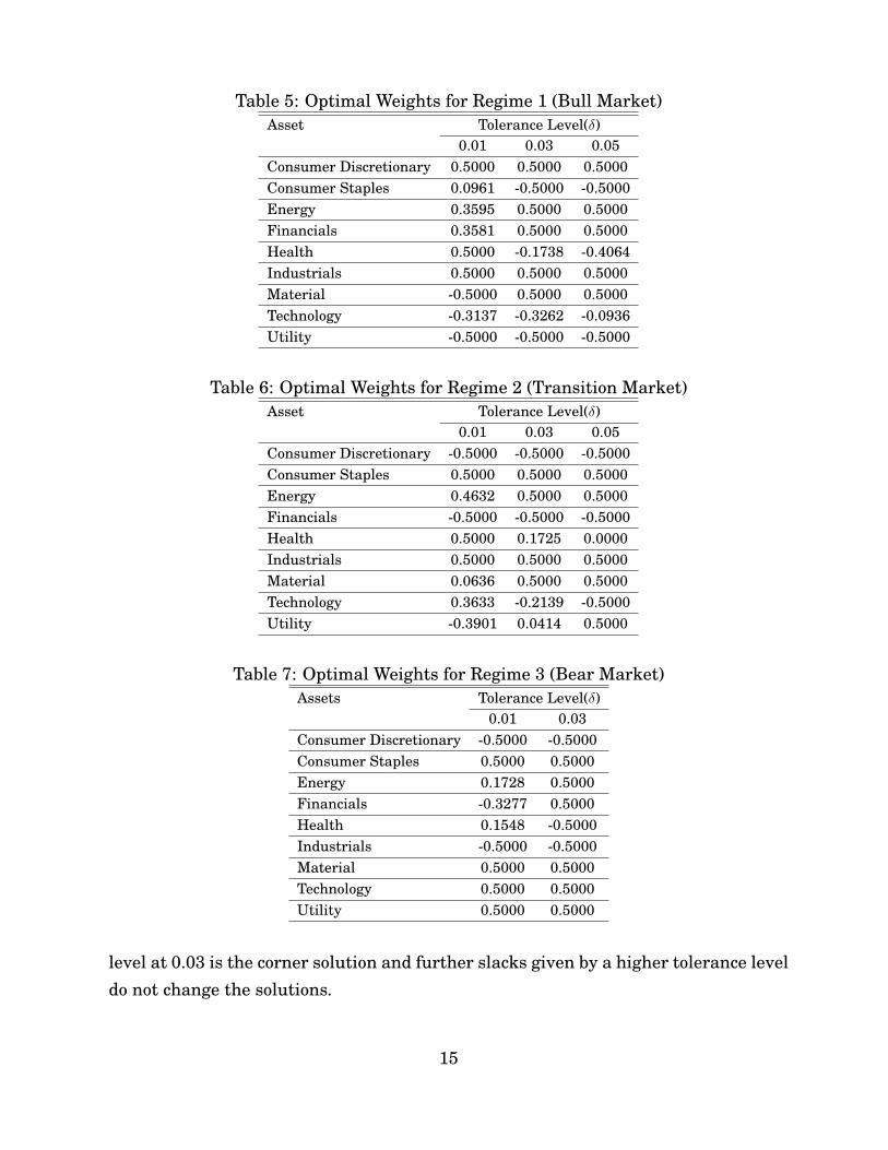
Using the estimates for alphas and betas, the stochastic linear programming problemis solved for the portfolio weights applicable to the next period (day). The limits oninvestment fractions ξl = −0.5 and ξu = 0.5 are imposed. This allows for a lot of varia-tion in the allocation of investment capital to the asset classes. At each decision point,the starting market regime is inferred based on the maximum posterior probabilityof the regimes, so the optimal portfolio weights are given by the starting regime. Asthe level of tolerance δ varies, the regime-dependent market neutral strategy sug-
13
Table 4: Alpha and Beta Estimates by RegimeRegime 1 BetaAsset Alpha MKT SMB HML VIX YS CS
gests different long and short positions for each regime. Tables 5, 6, and 7 provide theoptimal portfolio weights for sector ETFs for the bull, transition, and bear markets.
Table 7 provides the optimal weights for regime 3 (bear market) with the tolerancelevel (δ) at 0.01 and 0.03, as the weights at the tolerance level at 0.05 are the same asthose with the tolerance level at 0.03. That is, the optimal weights with the tolerance
level at 0.03 is the corner solution and further slacks given by a higher tolerance leveldo not change the solutions.
15
As the risk tolerance is relaxed the portfolio weights move to the limits. In fact, forthe transition and bear markets the boundary solution is optimal for lower tolerancelevels. It is in the bull market, where the trade-off between risk and return is greater,that solutions are more sensitive to the beta tolerance level. In each of the regimesshort selling some sector ETFs provides capital to invest in more promising sectorETFs.
5 Portfolio Performance
The regime-dependent strategies will be implemented for the ETFs during the periodfrom February 27, 2009 to September 30, 2009, a period of 150 trading days. At thestart of a day the implied regime (from the Viterbi (1967) algorithm) is considered tobe the true regime and the regime-dependent strategy is implemented. This strategyis then compared with the benchmark strategy, a popular approach to diversificationwith fixed portfolio weights over the investment horizon. Wealth is accumulated fromthe actual daily returns for ETFs during the study period.
Table 8 shows the mean, variance, standard deviation and Sharpe ratio of portfolioreturns under the regime-dependent strategy and benchmark strategy for the periodfrom February 27, 2009 to September 30. 2009.
For mean returns (either excess returns or cumulative returns), the portfolio per-formance under the regime-dependent strategy dominates that of the benchmarkstrategy, but with greater standard deviation (risk).
By examining the Sharpe ratio, we can get a picture of excess returns per unitof risk. The Sharpe ratio I in Table 8 is defined by the difference of portfolio re-turns under the regime-dependent strategy and the benchmark strategy divided bythe standard deviation of the difference of these returns. These Sharpe ratios are allpositive and suggest that the returns earned by the regime-dependent strategy arenot due to excess risk.
The Sharpe ratio II is defined by the difference of mean returns between the port-folio and a three month T-Bill yield divided by the standard deviation of the portfolioreturn. For either excess return or cumulative return, the Shape ratio II of the portfo-lio the under regime-dependent strategy is much higher than that of the benchmarkstrategy.
The regime in each day is implied by the analysis, and the performance in each
16
Table 8: Overall Performances
Panel A Tolerance Level=0.01Excess Return Cumulative Return
Portfolio Benchmark Portfolio BenchmarkMean 0.0032 0.0024 1.0904 1.0752Variance 0.0007 0.0003 0.0134 0.0073Standard Deviation 0.0273 0.0173 0.1160 0.0853Sharpe Ratio (I) 0.0530 0.3780Sharpe Ratio (II) 0.0551 0.0388 0.1086 -0.0304
Panel B Tolerance Level=0.03Excess Return Cumulative Return
Portfolio Benchmark Portfolio BenchmarkMean 0.0050 0.0024 1.1404 1.0752Variance 0.0015 0.0003 0.0465 0.0073Standard Deviation 0.0390 0.0173 0.2156 0.0853Sharpe Ratio (I) 0.1050 0.4480Sharpe Ratio (II) 0.0846 0.0388 0.2902 -0.0304
Panel C Tolerance Level=0.05Excess Return Cumulative Return
Portfolio Benchmark Portfolio BenchmarkMean 0.0052 0.0024 1.1534 1.0752Variance 0.0016 0.0003 0.0511 0.0073Standard Deviation 0.0402 0.0173 0.2260 0.0853Sharpe Ratio (I) 0.1050 0.4920Sharpe Ratio (II) 0.0854 0.0388 0.3345 -0.0304
regime can be calculated. Table 9 lists the portfolio performance statistics underregime-dependent strategy in the bull market. Compared to the overall portfolio per-formance, the portfolio performance for the bull market is similar but presents highermean returns, volatilities and Sharpe ratios.
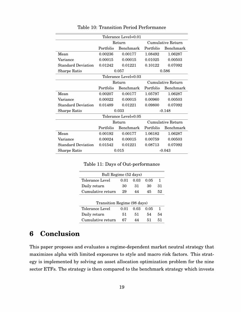
The only other regime in the study period was the “transition” market and thestatistics for that implied regime are provided in Table 10. The advantage of theregime-dependent strategy is not so obvious in this case.
An interesting issue is the number of days in the study period that the regime-dependent strategy outperforms the benchmark strategy. This result is shown inTable 11.
In the overall experiment period, 52 out of 150 days are in the bull market. In thebull market, about 60% of the time the regime-dependent strategy out-performs thebenchmark at each tolerance level. If cumulative returns are considered, where the
excess returns are carried forward, the percentage of days with out-performance ismuch higher, more in the order of 85%.
For the days in the transition market (98 days), the out-performance is about 50%of the time and this is consistent with the comparable statistics for both strategies inthat regime.
This paper proposes and evaluates a regime-dependent market neutral strategy thatmaximizes alpha with limited exposures to style and macro risk factors. This strat-egy is implemented by solving an asset allocation optimization problem for the ninesector ETFs. The strategy is then compared to the benchmark strategy which invests
19
passively and equally among the nine sector ETFs. In general, the regime-dependentstrategy outperforms the benchmark strategy. The regime-dependent strategy ap-pears to be much more attractive in the bull market than in the transition market,as its mean returns and Sharpe ratios are much higher in that market. In the transi-tion market, the regime-dependent strategy also slightly outperforms the benchmarkstrategy. In our evaluation period, the bear market is not present.
20
References
[1] A. Ang and G. Bekaert, International Asset Allocation with Regime Shifts, Re-view of Financial Studies. 20 (2002) 1137 – 1187.
[2] A. Ang and G. Bekaert, How regimes affect asset allocation, Financial AnalystsJournal. 60 (2004) 86–98.
[3] J-P. Berdot, D. Goyeau and J. Leonard, The dynamics of portfolio management:Exchange rate effects and multisector allocation, International Journal of Busi-ness. 11 (2006) 188–209.
[4] G. Berkaert and R.J. Hodrick, On biases in the measure of foreign exchange riskpremiums, Journal of International Money and Finance. 12 (1993) 115–138.
[5] J.W. Bronson, M.H. Scanlan and J. R. Squires, Managing individual investorportfolios, Managing Investor Portfolios: A Dynamic Process. 3rd edition, CFAInstitute, 2007.
[6] J. Cai, A Markov model of switching-regime ARCH, Journal of Business andEconomic Statistics. 12 (1994) 309–316
[7] D. Capocci, Neutrality of market neutral funds, Global Finance Journal. 17(2006) 309–333.
[8] N-F. Chen, R. Roll and S. Ross, Economic forces and the stock market, Journalof Business. 59 (1986) 383–403.
[9] A.P. Dempster, N.M. Laird and D.B. Rubin, Maximum likelihood from incompletedata via the EM algorithm, Journal of the Royal Statistical Society, Series B. 39(1977) 1–38.
[10] F.R. Edwards and M.O. Caglayan, Hedge fund performance and manager skill,Journal of Futures Markets. 21 (2001) 1003–1028.
[11] E. Fama and K.R. French, Common risk factors in the returns on stocks andbonds, Journal of Financial Economics. 33 (1993) 3–56.
[12] G.L. Gastineau, A.R. Olma and G. Robert, Equity portfolio management, Man-aging Investor Portfolios: A Dynamic Process. 3rd edition, CFA Institute, 2007.
21
[13] S.F. Gray, Modeling the conditional distribution of interest rates as a regime-switching process, Journal of Finacial Economics. 42 (1996) 27–62.
[14] M. Guidolin and A. Timmermann, Asset allocation under multivariate regimeswitching, Journal of Economic Dynamics and Control. 31 (2007) 3503–3544.
[15] M. Guidolin and A. Timmermann, International asset allocation under regimeswitching, skew and kurtosis preferences, Review of Financial Studies. 21 (2008)889–935.
[16] J.D. Hamilton, A new approach to the economic analysis of nonstationary timeseries and the business cycle, Econometrica. 57 (1989) 357–384.
[17] J.D. Hamilton, Rational-expectations econometric analysis of changes in regime:An investigation of the term structure of interest rates. Journal of EconomicDynamics and Control. 12(1998) 385–423.
[18] P. Liu, K. Xu and Y. Zhao, Market regimes, sectorial investments, and time-varying risk premiums, International Journal of Managerial Finance. 7 (2011),forthcoming.
[19] H.M. Markowitz, Portfolio selection, The Journal of Finance. 7 (1952) 77–91.
[20] S.M. Schaefer and I.A. Strebulaev, Structural models of credit risk are useful:Evidence from hedge ratios on corporate bonds, Journal of Financial Economics.90 (2008) 1–19.
[21] G.E. Schwarz, Estimating the dimension of a model, Annals of Statistics. 6 (1978)461-464.
[22] G. W. Schwert, Business cycles, financial crises, and stock volatility, Carnegie-Rochester Conference Series on Public Policy. 31 (1989) 82–126.
[23] S. Shyu, Y. Jeng, W.H. Ton, K. Lee and H.M. Chuang, Taiwan multi-factor modelconstruction: Equity market neutral strategies application, Managerial Finance.32 (2006) 915–947.
[24] J. Tu, Is regime switching in stock return important in portfolio decision? Man-agement Science. 56 (2010) 1198–1215.
22
[25] A.J. Viterbi, Error bounds for convolutional codes and an asymptotically opti-mum decoding algorithm. IEEE Transactions on Information Theory. 13 (1967)260–269.
[26] R. Whitelaw, Stock market risk and return: An equilibrium approach, Review ofFinancial Studies. 13 (2001) 521–548.