Affine-invariant geodesic geometry of deformable 3D shapes

Dan Raviv1, Alexander M. Bronstein2, Michael M. Bronstein3, Ron Kimmel1 and Nir Sochen4

1 Dept. of Computer Science, Technion, Israel, {darav,ron}@cs.technion.ac.il2 Dept. of Electrical Engineering, Tel Aviv University, Israel, bron@eng.tau.ac.il3 Institute of Computational Science, Faculty of Informatics, Universita della Svizzera Italiana, Lugano, michael.bronstein@usi.ch4 Dept. of Applied Mathematics, Tel Aviv University, Israel, sochen@math.tau.ac.il

Abstract

Natural objects can be subject to various transformations yet still preserve properties that we refer to as invariants.Here, we use definitions of affine invariant arclength for surfaces in R3 in order to extend the set of existing non-rigidshape analysis tools. We show that by re-defining the surface metric as its equi-affine version, the surface with itsmodified metric tensor can be treated as a canonical Euclidean object on which most classical Euclidean processingand analysis tools can be applied. The new definition of a metric is used to extend the fast marching method techniquefor computing geodesic distances on surfaces, where now, the distances are defined with respect to an affine invariantarclength. Applications of the proposed framework demonstrate its invariance, efficiency, and accuracy in shapeanalysis.

1. Introduction

Modeling 3D shapes as Riemannian manifold is aubiquitous approach in many shape analysis applica-tions. In particular, in the recent decade, shape de-scriptors based on geodesic distances induced by a Rie-mannian metric have become popular. Notable ex-amples of such methods are the canonical forms [7]and the Gromov-Hausdorff [9, 14, 2] and the Gromov-Wasserstein [13, 6] frameworks, used in shape compar-ison and correspondence problems. Such methods con-sider shapes as metric spaces endowed with a geodesicdistance metric, and pose the problem of shape similar-ity as finding the minimum-distortion correspondencebetween the metrics. The advantage of the geodesicdistances is their invariance to inelastic deformations(bendings) that preserve the Riemannian metric, whichmakes them especially appealing for non-rigid shapeanalysis. A particular setting of finding shape self-similarity can be used for intrinsic symmetry detectionin non-rigid shapes [17, 25, 12, 24].

The flexibility in the definition of the Riemannian

metric allows extending the invariance of the afore-mentioned shape analysis algorithms by constructing ageodesic metric that is also invariant to global transfor-mations of the embedding space. A particularly gen-eral and important class of such transformations are theaffine transformations. Such transformations are a com-mon local model for perspective distortions in images[15], and affine invariance is a necessary property ofimage descriptors. In 3D shape analysis, global affinetransformations play an important role in paleontologi-cal research studying bones of prehistoric creatures thatmay be squeezed by earth pressure [8]. Furthermore,photometric properties of 3D shapes and images can betreated as embedding coordinates in high-dimensionalspaces that include both geometric and color coordi-nates [20, 11]. Photometric transformations can be thusrepresented as geometric transformations of the respec-tive coordinates ,for example, affine transformations inthe Lab color space correspond to brightness, contrast,hue, and saturation transformations. Affine-invariantmetrics are thus useful for a description of the objectthat is invariant to color transformations.

Preprint submitted to SMI 2011 March 13, 2011

Many frameworks have been suggested to cope withthe action of the affine group in a global manner, try-ing to undo the affine transformation in large parts ofa shape or a picture. While the theory of affine invari-ance is known for many years [4] and used for curves[18] and flows [19], no numerical constructions appli-cable to general two-dimensional manifolds have beenproposed.

In this paper, we construct an (equi-)affine-invariantRiemannian geometry for 3D shapes. So far, such met-rics have been defined for convex surfaces; we extendthe construction to surfaces with non-vanishing Gaus-sian curvature. By defining an affine-invariant Rie-mannian metric, we can in turn define affine-invariantgeodesics, which result in a metric space with a strongerclass of invariance. This new metric allows us to de-velop efficient computational tools that handle non-rigiddeformations as well as equi-affine transformations. Wedemonstrate the usefulness of our construction in arange of shape analysis applications, such as shape pro-cessing, construction of shape descriptors, correspon-dence, and symmetry detection.

2. Background

We model a shape (X, g) as a compact complete two-dimensional Riemannian manifold (surface) X with ametric tensor g. The metric g can be identified withan inner product 〈·, ·〉x : TxX × TxX → R on the tan-gent plane TxX at point x. We further assume thatX is embedded into R3 by means of a regular mapx : U ⊆ R2 → R3, so that the metric tensor can beexpressed in coordinates as

gi j =∂xT

∂ui

∂x∂u j

, (1)

where ui are the coordinates of U.The metric tensor relates infinitesimal displacements

in the parametrization domain U to displacement on themanifold

dp2 = g11du12 + 2g12du1du2 + g22du2

2. (2)

This, in turn, provides a way to measure length struc-tures on the manifold. Given a curve C : [0,T ]→ X, itslength can be expressed as

`(C) =

∫ T

0〈C(t), C(t)〉1/2C(t)dt, (3)

where C denotes the velocity vector.

2.1. GeodesicsMinimal geodesics are the minimizers of `(C), giving

rise to the geodesic distances

dX(x, x′) = minC∈Γ(x,x′)

`(C) (4)

where Γ(x, x′) is the set of all admissible paths betweenthe points x and x′ on the surface X, where due to com-pleteness assumption, the minimizer always exists.

Structures expressible solely in terms of the metrictensor g are called intrinsic. For example, the geodesiccan be expressed in this way. The importance of intrin-sic structures stems from the fact that they are invari-ant under isometric transformations (bendings) of theshape. In an isometrically bent shape, the geodesic dis-tances are preserved – a property allowing to use suchstructures as invariant shape descriptors [7].

2.2. Fast marchingThe geodesic distance dX(x0, x) can be obtained as

the viscosity solution to the eikonal equation ‖∇d‖2 = 1(i.e., the largest d satisfying ‖∇d‖2 ≤ 1) with bound-ary condition at the source point d(x0) = 0. In thediscrete setting, a family of algorithms for finding theviscosity solution of the discretized eikonal equation bysimulated wavefront propagation is called fast march-ing methods [10]. On a discrete shape represented as atriangular mesh with N vertices, the general structureof fast marching closely resembles that of the classi-cal Dijkstra’s algorithm for shortest path computation ingraphs, with the main difference in the update step. Un-like the graph case where shortest paths are restricted topass through the graph edges, the continuous approxi-mation allows paths passing anywhere in the mesh tri-angles. For that reason, the value of d(x0, x) has to becomputed from the values of the distance map at twoother vertices forming a triangle with x. Computationof the distance map from a single source point has thecomplexity of O(N log N) [23]. On parametric surfaces,the fast marching can be carried out by means of a rasterscan and efficiently parallelized, which makes it espe-cially attractive for GPU-based computation [21, 3].

3. Affine-invariant geometry

An affine transformation x 7→ Ax + b of the three-dimensional Euclidean space can be parametrized usingtwelve parameters: nine for the linear transformationA, and additional three, b, for a translation, which wewill omit in the following discussion (here, we assumevectors to be column). Volume-preserving transforma-tions, known as special or equi-affine are restricted by

2

det A = 1. Such transformations involve only elevenparameters. In the following, when referring to affinetransformations and affine invariance, we will implyvolume-preserving (equi-)affine transformations.

An equi-affine metric can be defined through theparametrization of a curve on the surface. Let C be thecoordinates of a curve on the surface X parametrized byp. By the chain rule,

Cp = x1du1

dp+ x2

du2

dp

Cpp = x1d2u1

dp2 + x2d2u2

dp2 + x11

(du1

dp

)2

+

2x12du1

dpdu2

dp+ x22

(du2

dp

)2

, (5)

where, for brevity, we denote xi = ∂x∂ui

, xi j = ∂2x∂ui∂u j

, Cp =

dCdp , and Cpp = d2C

dp2 . As volumes are preserved underthe equi-affine group of transformations, we define theinvariant arclength p through

f (X) det(x1, x2,Cpp) = 1, (6)

where f (X) is a normalization factor for parameteri-zation invariance (i.e., invariance with respect to thechoice of p), and the determinant is applied on a matrixformed by the column vectors x1, x2, and Cpp. Since xi

is parallel to xiduidp it follows that

det(x1, x2, αx1 + βx2) = 0 ∀α , β, (7)

and plugging (5) into (6) using (7) yields the equi-affinearclength

dp2 = f (X) det(x1, x2, x11du21 +

2x12du1du2 + x22du22)

= f (X)(g11du2

1 + 2g12du1u2 + g22du22

),(8)

where gi j = det(x1, x2, xi j).In order to evaluate f (X) such that the quadratic form

(8) will also be parameterization invariant, we introducean arbitrary parameterization u1 and u2, for which xi =∂x∂ui

and xi j = ∂2x∂ui∂u j

. The relation between the two sets ofparameterizations can be expressed using the chain rule

x1 = xu1 = xu1 u1u1 + xu2 u2u1 (9)x2 = xu2 = xu1 u1u2 + xu2 u2u2 .

It can be shown [1, 4] using the Jacobian

J =

(u1u1 u2u1

u1u2 u2u2

), (10)

that

g11du21 + 2g12du1du2 + g22du2

2

=(g11du2 + 2g12dudv + g22dv2

)det(J), (11)

and

g11g22 − g212 =

(g11g22 − g2

12

)det4(J), (12)

where gi j = det(x1, x2, xi j). From (11) and (12) we con-clude that

g11du21 + 2g12du1du2 + g22du2

2∣∣∣g11g22 − g212

∣∣∣ 14

=g11du2 + 2g12dudv + g22dv2∣∣∣g11g22 − g2

12

∣∣∣ 14

, (13)

and derive the affine invariant parameter normalization

f (X) = |g|−1/4 , (14)

which defines the equi-affine pre-metric tensor [4, 19]

gi j = gi j |g|−1/4 . (15)

The pre-metric tensor (15) applies only for strictlyconvex surfaces [4]; a similar difficulty appeared inequi-affine curve evolution. There the arc-length wasdetermined by the absolute value of the geometric struc-ture [18]. In two dimensions the problem is more acuteas we can encounter non-positive definite metrics inconcave, and hyperbolic regions.

We propose fixing the metric by flipping the mainaxes of the operator, if needed. In practice, we restrictthe eigenvalues of the tensor to be positive. From theeigendecomposition in matrix notation, G = UΓUT ofg where U is orthogonal and Γ = diag{γ1, γ2}, we com-pose a new metric G, such that

G = U|Γ|UT (16)

is positive definite and equi-affine invariant, for surfaceswith non-vanishing Gaussian curvature.

4. Discretization

We model the surface X as a triangular mesh, andconstruct three coordinate functions x(u, v), y(u, v), andz(u, v) for each triangle. While this can be done prac-tically in any representation, we use the fact that a tri-angle and its three adjacent neighbors, can be unfoldedto the plane, and produce a parameter domain. The co-ordinates of this planar representation are used as theparametrization with respect to which the first funda-mental form coefficients are computed at the barycenter

3

Standard Equi-affine

Standard Equi-affine

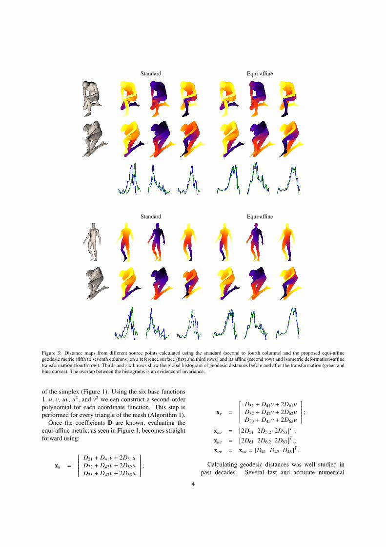
Figure 3: Distance maps from different source points calculated using the standard (second to fourth columns) and the proposed equi-affinegeodesic metric (fifth to seventh columns) on a reference surface (first and third rows) and its affine (second row) and isometric deformation+affinetransformation (fourth row). Thirds and sixth rows show the global histogram of geodesic distances before and after the transformation (green andblue curves). The overlap between the histograms is an evidence of invariance.

of the simplex (Figure 1). Using the six base functions1, u, v, uv, u2, and v2 we can construct a second-orderpolynomial for each coordinate function. This step isperformed for every triangle of the mesh (Algorithm 1).

Once the coefficients D are known, evaluating theequi-affine metric, as seen in Figure 1, becomes straightforward using:

xu =

D21 + D41v + 2D51uD22 + D42v + 2D52uD23 + D43v + 2D53u

;

xv =

D31 + D41v + 2D61uD32 + D42v + 2D62uD33 + D43v + 2D63u

;

xuu =[2D51 2D5,2 2D53

]T ;xuu =

[2D61 2D6,2 2D63

]T ;xuv = xvu = [D41 D42 D43]T .

Calculating geodesic distances was well studied inpast decades. Several fast and accurate numerical

4

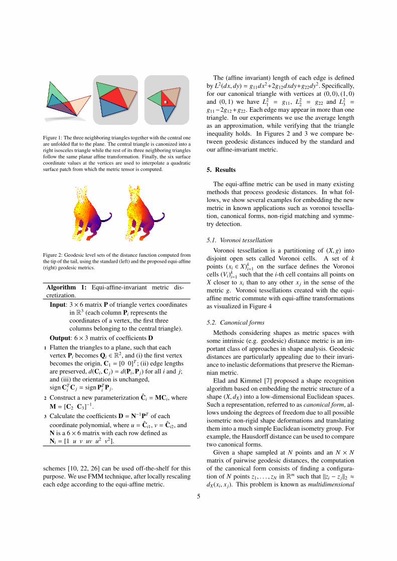
Figure 1: The three neighboring triangles together with the central oneare unfolded flat to the plane. The central triangle is canonized into aright isosceles triangle while the rest of its three neighboring trianglesfollow the same planar affine transformation. Finally, the six surfacecoordinate values at the vertices are used to interpolate a quadraticsurface patch from which the metric tensor is computed.

Figure 2: Geodesic level sets of the distance function computed fromthe tip of the tail, using the standard (left) and the proposed equi-affine(right) geodesic metrics.

Algorithm 1: Equi-affine-invariant metric dis-cretization.

Input: 3 × 6 matrix P of triangle vertex coordinatesin R3 (each column Pi represents thecoordinates of a vertex, the first threecolumns belonging to the central triangle).

Output: 6 × 3 matrix of coefficients D1 Flatten the triangles to a plane, such that each

vertex Pi becomes Qi ∈ R2, and (i) the first vertexbecomes the origin, C1 = [0 0]T ; (ii) edge lengthsare preserved, d(Ci,C j) = d(Pi,P j) for all i and j;and (iii) the orientation is unchanged,sign CT

i C j = sign PTi P j.

2 Construct a new parameterization Ci = MCi, whereM = [C2 C3]−1.

3 Calculate the coefficients D = N−1PT of eachcoordinate polynomial, where u = Ci1, v = Ci2, andN is a 6 × 6 matrix with each row defined asNi = [1 u v uv u2 v2].

schemes [10, 22, 26] can be used off-the-shelf for thispurpose. We use FMM technique, after locally rescalingeach edge according to the equi-affine metric.

The (affine invariant) length of each edge is definedby L2(dx, dy) = g11dx2+2g12dxdy+g22dy2. Specifically,for our canonical triangle with vertices at (0, 0), (1, 0)and (0, 1) we have L2

1 = g11, L22 = g22 and L2

3 =

g11−2g12 +g22. Each edge may appear in more than onetriangle. In our experiments we use the average lengthas an approximation, while verifying that the triangleinequality holds. In Figures 2 and 3 we compare be-tween geodesic distances induced by the standard andour affine-invariant metric.

5. Results

The equi-affine metric can be used in many existingmethods that process geodesic distances. In what fol-lows, we show several examples for embedding the newmetric in known applications such as voronoi tessella-tion, canonical forms, non-rigid matching and symme-try detection.

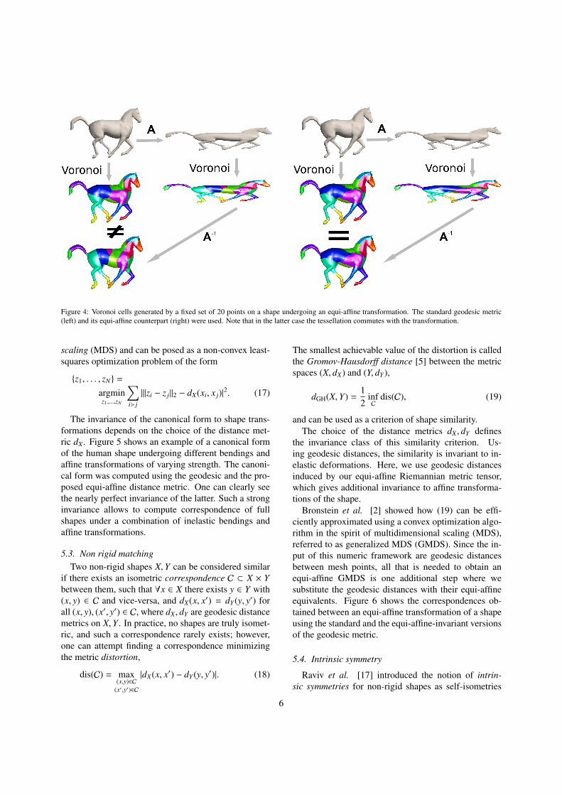
5.1. Voronoi tessellation

Voronoi tessellation is a partitioning of (X, g) intodisjoint open sets called Voronoi cells. A set of kpoints (xi ∈ X)k

i=1 on the surface defines the Voronoicells (Vi)k

i=1 such that the i-th cell contains all points onX closer to xi than to any other x j in the sense of themetric g. Voronoi tessellations created with the equi-affine metric commute with equi-affine transformationsas visualized in Figure 4

5.2. Canonical forms

Methods considering shapes as metric spaces withsome intrinsic (e.g. geodesic) distance metric is an im-portant class of approaches in shape analysis. Geodesicdistances are particularly appealing due to their invari-ance to inelastic deformations that preserve the Rieman-nian metric.

Elad and Kimmel [7] proposed a shape recognitionalgorithm based on embedding the metric structure of ashape (X, dX) into a low-dimensional Euclidean spaces.Such a representation, referred to as canonical form, al-lows undoing the degrees of freedom due to all possibleisometric non-rigid shape deformations and translatingthem into a much simple Euclidean isometry group. Forexample, the Hausdorff distance can be used to comparetwo canonical forms.

Given a shape sampled at N points and an N × Nmatrix of pairwise geodesic distances, the computationof the canonical form consists of finding a configura-tion of N points z1, . . . , zN in Rm such that ‖zi − z j‖2 ≈

dX(xi, x j). This problem is known as multidimensional

5

Figure 4: Voronoi cells generated by a fixed set of 20 points on a shape undergoing an equi-affine transformation. The standard geodesic metric(left) and its equi-affine counterpart (right) were used. Note that in the latter case the tessellation commutes with the transformation.

scaling (MDS) and can be posed as a non-convex least-squares optimization problem of the form

{z1, . . . , zN} =

argminz1,...,zN

∑i> j

|‖zi − z j‖2 − dX(xi, x j)|2. (17)

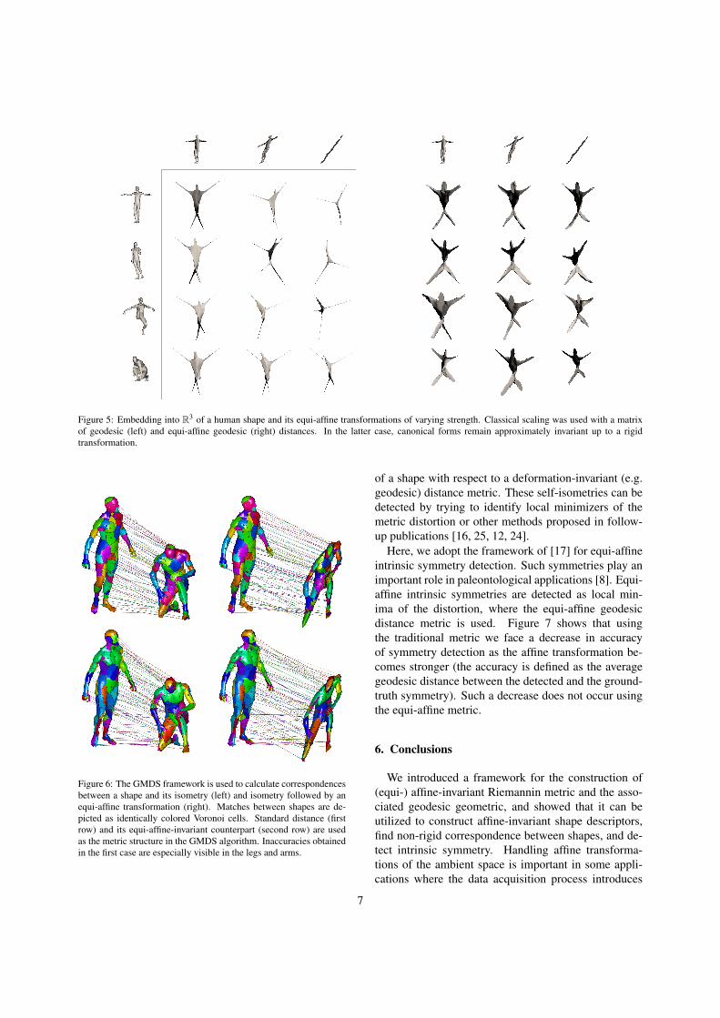
The invariance of the canonical form to shape trans-formations depends on the choice of the distance met-ric dX . Figure 5 shows an example of a canonical formof the human shape undergoing different bendings andaffine transformations of varying strength. The canoni-cal form was computed using the geodesic and the pro-posed equi-affine distance metric. One can clearly seethe nearly perfect invariance of the latter. Such a stronginvariance allows to compute correspondence of fullshapes under a combination of inelastic bendings andaffine transformations.

5.3. Non rigid matchingTwo non-rigid shapes X,Y can be considered similar

if there exists an isometric correspondence C ⊂ X × Ybetween them, such that ∀x ∈ X there exists y ∈ Y with(x, y) ∈ C and vice-versa, and dX(x, x′) = dY (y, y′) forall (x, y), (x′, y′) ∈ C, where dX , dY are geodesic distancemetrics on X,Y . In practice, no shapes are truly isomet-ric, and such a correspondence rarely exists; however,one can attempt finding a correspondence minimizingthe metric distortion,

dis(C) = max(x,y)∈C

(x′,y′)∈C

|dX(x, x′) − dY (y, y′)|. (18)

The smallest achievable value of the distortion is calledthe Gromov-Hausdorff distance [5] between the metricspaces (X, dX) and (Y, dY ),

dGH(X,Y) =12

infC

dis(C), (19)

and can be used as a criterion of shape similarity.The choice of the distance metrics dX , dY defines

the invariance class of this similarity criterion. Us-ing geodesic distances, the similarity is invariant to in-elastic deformations. Here, we use geodesic distancesinduced by our equi-affine Riemannian metric tensor,which gives additional invariance to affine transforma-tions of the shape.

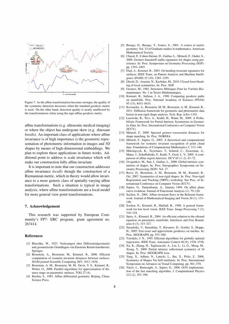
Bronstein et al. [2] showed how (19) can be effi-ciently approximated using a convex optimization algo-rithm in the spirit of multidimensional scaling (MDS),referred to as generalized MDS (GMDS). Since the in-put of this numeric framework are geodesic distancesbetween mesh points, all that is needed to obtain anequi-affine GMDS is one additional step where wesubstitute the geodesic distances with their equi-affineequivalents. Figure 6 shows the correspondences ob-tained between an equi-affine transformation of a shapeusing the standard and the equi-affine-invariant versionsof the geodesic metric.

5.4. Intrinsic symmetry

Raviv et al. [17] introduced the notion of intrin-sic symmetries for non-rigid shapes as self-isometries

6

Figure 5: Embedding into R3 of a human shape and its equi-affine transformations of varying strength. Classical scaling was used with a matrixof geodesic (left) and equi-affine geodesic (right) distances. In the latter case, canonical forms remain approximately invariant up to a rigidtransformation.

Figure 6: The GMDS framework is used to calculate correspondencesbetween a shape and its isometry (left) and isometry followed by anequi-affine transformation (right). Matches between shapes are de-picted as identically colored Voronoi cells. Standard distance (firstrow) and its equi-affine-invariant counterpart (second row) are usedas the metric structure in the GMDS algorithm. Inaccuracies obtainedin the first case are especially visible in the legs and arms.

of a shape with respect to a deformation-invariant (e.g.geodesic) distance metric. These self-isometries can bedetected by trying to identify local minimizers of themetric distortion or other methods proposed in follow-up publications [16, 25, 12, 24].

Here, we adopt the framework of [17] for equi-affineintrinsic symmetry detection. Such symmetries play animportant role in paleontological applications [8]. Equi-affine intrinsic symmetries are detected as local min-ima of the distortion, where the equi-affine geodesicdistance metric is used. Figure 7 shows that usingthe traditional metric we face a decrease in accuracyof symmetry detection as the affine transformation be-comes stronger (the accuracy is defined as the averagegeodesic distance between the detected and the ground-truth symmetry). Such a decrease does not occur usingthe equi-affine metric.

6. Conclusions

We introduced a framework for the construction of(equi-) affine-invariant Riemannin metric and the asso-ciated geodesic geometric, and showed that it can beutilized to construct affine-invariant shape descriptors,find non-rigid correspondence between shapes, and de-tect intrinsic symmetry. Handling affine transforma-tions of the ambient space is important in some appli-cations where the data acquisition process introduces

7

Figure 7: As the affine transformation becomes stronger, the quality ofthe symmetry detection decreases when the standard geodesic metricis used. On the other hand, detection quality is nearly unaffected bythe transformations when using the equi-affine geodesic metric.

affine transformations (e.g. ultrasonic medical imaging)or where the object has undergone skew (e.g. dinosaurfossils). An important class of applications where affineinvariance is of high importance is the geometric repre-sentation of photometric information in images and 3Dshapes by means of high-dimensional embeddings. Weplan to explore these applications in future works. Ad-ditional point to address is scale invariance which willmake our construction fully affine-invariant.

It is important to note that our construction addressesaffine invariance locally though the construction of aRiemannian metric, which in theory would allow invari-ance to a more generic class of spatially-varying affinetransformations. Such a situation is typical in imageanalysis, where affine transformations are a local modelfor more general view point transformations.

7. Acknowledgement

This research was supported by European Com-munity’s FP7- ERC program, grant agreement no.267414.

References

[1] Blaschke, W., 1923. Vorlesungen uber Differentialgeometricund geometrische Grundlagen von Einsteins Relativitatstheorie.Springer.

[2] Bronstein, A., Bronstein, M., Kimmel, R., 2006. Efficientcomputation of isometry-invarient distances between surfaces.SIAM journal Scientific Computing 28/5, 1812–1836.

[3] Bronstein, A. M., Bronstein, M. M., Devir, Y. S., Kimmel, R.,Weber, O., 2008. Parallel algorithms for approximation of dis-tance maps on parametric surfaces. TOG 27 (4).

[4] Buchin, S., 1983. Affine differential geometry. Beijing, China:Science Press.

[5] Burago, D., Burago, Y., Ivanov, S., 2001. A course in metricgeometry. Vol. 33 of Graduate studies in mathematics. AmericanMathematical Society.

[6] Chazal, F., Cohen-Steiner, D., Guibas, L., Memoli, F., Oudot, S.,2009. Gromov-hausdorff stable signatures for shapes using per-sistence. In: Proc. Symposium on Geometry Processing (SGP).pp. 1393–1403.

[7] Elad, A., Kimmel, R., 2003. On bending invariant signatures forsurfaces. IEEE Trans. on Pattern Analysis and Machine Intelli-gence (PAMI) 25 (10), 1285–1295.

[8] Ghosh, D., Amenta, N., Kazhdan, M., 2010. Closed-form blend-ing of local symmetries. In: Proc. SGP.

[9] Gromov, M., 1981. Structures Metriques Pour les Varietes Rie-manniennes. No. 1 in Textes Mathematiques.

[10] Kimmel, R., Sethian, J. A., 1998. Computing geodesic pathson manifolds. Proc. National Academy of Sciences (PNAS)95 (15), 8431–8435.

[11] Kovnatsky, A., Bronstein, M. M., Bronstein, A. M., Kimmel, R.,2011. Diffusion framework for geometric and photometric datafusion in non-rigid shape analysis. Tech. Rep. arXiv:1101.

[12] Lasowski, R., Tevs, A., Seidel, H., Wand, M., 2009. A Proba-bilistic Framework for Partial Intrinsic Symmetries in Geomet-ric Data. In: Proc. International Conference on Computer Vision(ICCV).

[13] Memoli, F., 2009. Spectral gromov-wasserstein distances forshape matching. In: Proc. NORDIA.

[14] Memoli, F., Sapiro, G., 2005. A theoretical and computationalframework for isometry invariant recognition of point clouddata. Foundations of Computational Mathematics 5, 313–346.

[15] Mikolajczyk, K., Tuytelaars, T., Schmid, C., Zisserman, A.,Matas, J., Schaffalitzky, F., Kadir, T., Gool, L. V., 2005. A com-parison of affine region detectors. IJCV 65 (1–2), 43–72.

[16] Ovsjanikov, M., Sun, J., Guibas, L., 2008. Global intrinsic sym-metries of shapes. In: Proc. Eurographics Symposium on Ge-ometry Processing (SGP). Vol. 27.

[17] Raviv, D., Bronstein, A. M., Bronstein, M. M., Kimmel, R.,Oct. 2007. Symmetries of non-rigid shapes. In: Proc. Non-rigidRegistration and Tracking (NRTL) workshop. See Proc. of In-ternational Conference on Computer Vision (ICCV).

[18] Sapiro, G., Tannenbaum, A., January 1994. On affine planecurve evolution. Journal of Functional Analysis (1), 79–120.

[19] Sochen, N., 2004. Affine-invariant flows in the Beltrami frame-work. Journal of Mathematical Imaging and Vision 20 (1), 133–146.

[20] Sochen, N., Kimmel, R., Malladi, R., 1998. A general frame-work for low level vision. IEEE Trans. Image Processing 7 (3),310–318.

[21] Spira, A., Kimmel, R., 2004. An efficient solution to the eikonalequation on parametric manifolds. Interfaces and Free Bound-aries 6 (3), 315–327.

[22] Surazhsky, V., Surazhsky, T., Kirsanov, D., Gortler, S., Hoppe,H., 2005. Fast exact and approximate geodesics on meshes. In:Proc. SIGGRAPH. pp. 553–560.

[23] Tsitsiklis, J. N., 1995. Efficient algorithms for globally optimaltrajectories. IEEE Trans. Automatic Control 40 (9), 1528–1538.

[24] Xu, K., Zhang, H., Tagliasacchi, A., Liu, L., Li, G., Meng, M.,Xiong, Y., 2009. Partial intrinsic reflectional symmetry of 3dshapes. In: Proc. SIGGRAPH Asia.

[25] Yang, X., Adluru, N., Latecki, L., Bai, X., Pizlo, Z., 2008.Symmetry of Shapes Via Self-similarity. In: Proc. InternationalSymposium on Advances in Visual Computing. pp. 561–570.

[26] Yatziv, L., Bartesaghi, A., Sapiro, G., 2006. O(N) implementa-tion of the fast marching algorithm. J. Computational Physics212 (2), 393–399.

8