Research ArticleAGA-Based BP Artificial Neural Network for EstimatingMonthlySurface Air Temperature of the Antarctic during 1960ndash2019
Miao Fang
Northwest Institute of Eco-Environment and Resource Chinese Academy of Sciences Lanzhou 730000 China
Correspondence should be addressed to Miao Fang mfanglzbaccn
Received 11 April 2021 Revised 12 May 2021 Accepted 1 June 2021 Published 7 June 2021
Academic Editor Pedro Jimenez-Guerrero
Copyright copy 2021 Miao Fang )is is an open access article distributed under the Creative Commons Attribution License whichpermits unrestricted use distribution and reproduction in any medium provided the original work is properly cited
)e spatial sparsity and temporal discontinuity of station-based SAT data do not allow to fully understand Antarctic surface airtemperature (SAT) variations over the last decades Generating spatiotemporally continuous SAT fields using spatial interpolationrepresents an approach to address this problem )is study proposed a backpropagation artificial neural network (BPANN)optimized by a genetic algorithm (GA) to estimate the monthly SAT fields of the Antarctic continent for the period 1960ndash2019Cross-validations demonstrate that the interpolation accuracy of GA-BPANN is higher than that of two benchmark methods ieBPANN and multiple linear regression (MLR))e errors of the three interpolation methods feature month-dependent variationsand tend to be lower (larger) in warm (cold) months Moreover the annual SAT had a significant cooling trend during 1960ndash1989(trend minus007degCyear p 004) and a significant warming trend during 1990ndash2019 (trend 006degCyear p 005) )e monthlySATdid not show consistent cooling or warming trends in all months eg SATdid not show a significant cooling trend in Januaryand December during 1960ndash1989 and a significant warming trend in January June July and December during 1990ndash2019Furthermore the Antarctic SAT decreases with latitude and the distance away from the coastline but the eastern Antarctic isoverall colder than the western Antarctic Spatiotemporal inconsistencies on SAT trends are apparent over the Antarcticcontinent eg most of the Antarctic continent showed a cooling trend during 1960ndash1989 (trend minus020sim0degCyearp 001 sim 027) with a peak over the central part of the eastern Antarctic continent while the entire Antarctic continent showed awarming trend during 1990ndash2019 (trend 0sim010degCyear p 004 sim 042) with a peak over the higher latitudes
1 Introduction
Variation in surface air temperature (SAT) over the Ant-arctic is an indicator of global SAT change [1] Variations inthe Antarctic SAT partly contribute to climate anomalies inEast Asia [2] Tropics [3] and Arctic [4] through the at-mosphere-ocean bridges Establishing how the AntarcticSAT modulates the sea ice extent and thickness over theSouthern Hemisphere will improve the predictability ofglobal climate change However challenges exist in un-derstanding the Antarctic SAT and previous studies havenot reached consistent conclusions Some studies have re-ported that most of the Antarctic continent has shown acooling trend [5ndash7] In contrast other studies support aweak warming trend over the entire Antarctic continent[8ndash10] In addition some studies have reported that the
Antarctic Peninsula showed a warming trend during the lastdecades of the twentieth century [11 12] but other researchsuggested that there was no evidence that the AntarcticPeninsula has experienced warming during that period [13]Among the factors responsible for the inconsistent studyresults are the sparsity and temporal discontinuity of station-based SAT data [14] the lack of good quality satellite-basedSAT products which are often affected by cloud cover andsnow surface over the Antarctic [15] the large warm bias inreproducing the Antarctic temperature using climate models[16] the clear cold bias for monthly SAT reanalysis datasetsover the Antarctic coastal regions and the large warm biasdominating the winter over the Antarctic inland [17] )eabove inconsistencies may also be attributed to the differentdata sources used for each study Accordingly generating awidely accepted high-quality and spatiotemporally
HindawiAdvances in MeteorologyVolume 2021 Article ID 8278579 14 pageshttpsdoiorg10115520218278579
continuous SATdataset over the Antarctic is critical to betterunderstand the Antarctic SAT variation during the lastdecades
An alternative approach is used to generate spatiotem-porally continuous and high-quality SAT data based onlimited station-based SAT observations and appropriatespatial interpolation methods [18 19] which allows ex-ploring the SAT variations over the areas where station-based data are not available )ere are many spatial inter-polation methods such as inverse distance weighting (IDW)[20] Spline method [21] Kriging-based method [22] andmultiple linear regression method [23] Based on thesemethods several gridded SATdatasets have been developedsuch as theMet OfficeHadley Centre Climatic Research UnitTemperature version 4 (hereinafter HadCRUT4) [24]Berkeley Earth Surface Temperatures (hereinafter BEST)[25] NASAGISS Surface Temperature Analysis (hereinafterGISTEMP) [26] NOAAMerged Land-Ocean Global SurfaceTemperature Analysis version 4 (MLOST) [27] and ClimaticResearch Unit Timeseries version 4 (CRU TS) [28] How-ever although these SAT datasets have been widely used invarious climate studies shortcomings persist For examplethese datasets do not cover some crucial regions and thereare large areas of missing values over the ocean and theAntarctic [29] )ese shortcomings motivated this researchto establish new approaches to create gridded SAT datasetscovering the entire Antarctic and meeting high-qualitystandards
In recent years machine learning- (ML-) based spatialinterpolation methods have been proposed over traditionalmethods (eg IDW Spline and Kriging) [30ndash33] )efeedforward backward-propagation artificial neural network(BPANN) [34] which is a commonly used ANN model inML is a promising tool for solving complex nonlinearmodelling and prediction problems [35] As a type ofnonlinear model BPANN can find the complex nonlinearrelationships within the sample data without assuming aspecific relationship between the input and output in ad-vance [34] )e BPANN algorithm has been used in thespatial interpolation of climate variables [36ndash38] Howeverdue to its purely data-driven characteristics BPANN alsoshowed deficiencies in practice For example BPANN isprone to overfitting [39] and can easily fall into local optimalsolutions [40] In addition the structure of BPANN cannotbe easily determined and while the selection of the initialconnection weights and thresholds of the network greatlyimpacts BPANNrsquos performance they are random andcannot be accurately obtained [41] Aiming to overcomethese intrinsic deficiencies many researchers have attemp-ted to improve BPANNrsquos performance using intelligentoptimization algorithms [42ndash45] Genetic algorithms (GA)feature excellent global search ability [46] and are used tooptimize the initial connection weights and thresholds ofBPANN (hereinafter GA-BPANN) in order to avoid fallinginto a local optimum and improve its training speed andmodelling ability [42 47] )erefore GA-BPANN has beenapplied in many fields of natural and social sciences forcomplex nonlinear modelling and prediction showing ex-cellent performance over other BPANN models optimized
by different algorithms [48ndash51] Currently however thereare very few reports on the use of GA-BPANN for spatialinterpolation especially for the interpolation of Antarctictemperatures
A high-quality and spatiotemporally continuous SATdataset is the foundation of Antarctic climate research )isstudy aims to produce a monthly gridded SATdataset for theAntarctic continent during 1960ndash2019 using the GA-BPANNmethod and limited station-based SAT observations )eperformance of the GA-BPANN for spatial interpolation iscompared with those of MLR and BPANN)e remainder ofthe paper is organized as follows )e details of the station-based SATdata and the spatial interpolation methods used inthis study are presented in Section 2 Section 3 includes thevalidation of the estimated Antarctic SAT datasets usingdifferent interpolation methods Preliminary analyses re-garding the spatiotemporal variations of the Antarctic SATduring 1960ndash2019 are also described in this section Someprospects for improving the data quality of the SAT inter-polation are discussed in Section 4 In the final section themain findings of this study are summarized
2 Data and Methods
21 Station-Based SAT Data )e station-based SAT data ofthe Antarctic were extracted from the Global HistoricalClimatology Network monthly dataset version 4 (hereinafterGHCNmV4) [52])eGHCNmV4 is a set ofmonthly climaterecords from thousands of weather stations around the world)e monthly data have periods of record that vary by stationwith the earliest observations dating to the eighteenth centurySome station records are purely historical and are no longerupdated whereas many others are still up to date Relative toprevious versions the GHCNmV4 provides an expandeddataset of station-based temperature records as well as morecomprehensive uncertainties for the calculation of station andregional temperature trends )e total number of monthlytemperature stations in GHCNmV4 over the Antarctic during1960ndash2019 is 82 (Figure 1)
22 Geographic Factor Data )e geographic factors af-fecting the spatial distribution of SAT mainly include lon-gitude latitude altitude topographic conditions and landcover [53] Previous studies have reported that the monthlymean SAT has a significant correlation with latitude lon-gitude and altitude [54 55] In addition the spatial dis-tribution of SAT at the continental scales is mainlycontrolled by geographic factors such as latitude longitudeand elevation [54] )ese three factors usually are extractedfrom digital elevation model (DEM) data In this study a1 km resolution Antarctic DEM data was used these datawere downloaded from the National Tibetan Plateau DataCentre (TPDC httpsdatatpdcaccnen) )is 1 km res-olution DEM can well capture the striking effect of Antarcticorography on SAT distributions )e elevation of each SATstation was extracted based on the longitude and latitude ofthis SAT station )e training sample used to construct thespatial interpolation model includes the longitudes and
2 Advances in Meteorology
latitudes of all SATstations the extracted elevations and themonthly SAT observations during 1960ndash2019 )e inter-polation model was constructed monthly using the trainingsample Additionally the longitudes latitudes and eleva-tions on all grids were obtained through DEM sampling inArcGIS software and then were used as the input sample ofthe monthly varied interpolation model for estimating themonthly SAT fields of the Antarctic continent during1960ndash2019 )erefore the spatial resolution of the estimatedSAT fields is consistent with that of DEM both of which are1 km regular grids
23 Spatial Interpolation Methods
231 MLR Multiple linear regression (MLR) is a com-monly used method in spatial interpolation and its per-formance is always superior to several benchmarkinterpolation methods such as IDW Spline and Kriging[23] In this study the MLR-based interpolation result isconsidered as a reference to compare the interpolationperformances of the BPANN andGA-BPANN According toprevious studies the MLR method considers that the spatialdistribution of SAT is the comprehensive effect of longitudelatitude altitude and other geographic factors MLR takesSAT as the dependent variable and geographic factors suchas altitude latitude and longitude as independent variables[20 56] to construct the SAT interpolation model as follows
T ax1 + bx2 + cx3 + ε (1)
where T denotes SAT and x1 x2 x3 are longitude latitudeand altitude respectively ε is the residual error a b c areregression coefficients )e regression coefficients and
residual error are estimated by the least square method )eMLR model is constructed and then the SAT over otherareas is estimated based on the constructed MLR model andthe longitudes latitudes and altitudes extracted from theDEM data
232 BPANN )e BPANN model is one of the mostcommonly used ANN models and has strong nonlinearmodelling and analysis capability for complex systemsBPANN uses a nonlinear differentiable function to train amultilayer network which is divided into input layerhidden layer and output layer BPANN features severaladvantages including (1) simple structures and easy op-erability (2) sophisticated nonlinear mapping from inputto output and (3) self-study ability for further improve-ment and development [57] In this study there were threeneurons in the input layer of the BPANN model to denotethe longitude latitude and altitude and one neuron in theoutput layer (ie the SAT) )e number of neurons in thehidden layer is a fundamental parameter of the BPANNmodel but it is difficult to determine exactly Currentlyempirical rules for addressing this problem have beenproposed [58] In this study the neurons of the hiddenlayer were set to seven according to these rules )estructure of BPANN is described in Figure 2 and takes thefollowing formulation
SAT BPANN(lontitude latitude altitude θ) + ε (2)
where ε is the residual error and θ denotes the parameters ofthe BPANN model such as connection weights andthresholds
30degE60degE
90degE
120degE
150degE
180degE
70degS
150degW120degW
90degW
60degW90degS
80degS
30degW
0deg
(a)
0
10
20
30
40
50
60
70
80
90
Num
ber o
f SA
T sta
tions
1920 1940 1960 19801900 20202000Year
JanFebMarApr
MayJunJulAug
SepOctNovDec
(b)
Figure 1 )e spatiotemporal distribution of the extracted station-based SAT data of the Antarctic
Advances in Meteorology 3
233 GA-BPANN A GA is a kind of self-adaptive andprobabilistic global searching process that starts from aninitial population of finite string representations in whicheach member (called chromosome or individual) representsa candidate solution to the problem [46] )e initial pop-ulation of a GA is randomly sampled A GA provides asolution space that enables BPANN to find the optimalsolution that helps avoid a local optimum In GA-BPANNeach individual (or chromosome) represents a distributionof connection weights and thresholds of each network)us a population of individuals (or chromosomes) rep-resents a population of neural networks with differentweights and threshold distributions A GA is used to op-timize the initial weights and thresholds of BPANN )eBPANN model optimized by GA includes two parts Onepart is to determine the BPANN structure and code theinitial individuals )e other part is to optimize BPANNwith GA )e GA process is summarized as follows (1)initialize the population (2) calculate the fitness value ofeach individual in the population (3) select individualswhich will enter the next generation according to a ruledetermined by individual fitness values (4) performcrossover operation according to crossover probability (5)carry out mutation operation according to mutationprobability (6) if the end conditions are not met then go tostep (2) or enter (7) and (7) use the individual (orchromosome) with the best fitness value in the output
population as the optimal solution of the problem As aresult the most optimal individual which represents theoptimal initial weights and thresholds of the BPANNmodel is generated Figure 3 describes the flowchart ofBPANN optimized with GA for the details of populationinitialization fitness function selection operation cross-over operation and for mutation operation refer to[46 47]
24 Validation Method Cross-validation was used toevaluate the spatial interpolation performances of the abovethree interpolation methods )e cross-validation assumesthat the SAT value of each station is unknown and is es-timated based on the SAT values of the surrounding sta-tions )e errors between the observed SAT values and theestimated SAT values of all stations are calculated toevaluate the performance of the interpolation methodTypical performance indicators including mean absoluteerror (MAE) and root-mean-square error (RMSE) wereused to investigate the differences between the observedSATand the estimated SAT )e MAE reflects the extent ofthe overall error at all sites while the RMSE can reflect theestimated sensitivity and extreme effect of the error sampledata Smaller values of these two metrics indicate higheraccuracy of the interpolation )e formulas for MAE andRMSE are as follows
Input layer Hidden layer Output layer
Actualinput
Actualoutput
Modelledoutput
O1 Y1
μk
μ1
Z1
μm
Ok
Vjk
Om
Zp
Zj
Xn
Xi
X1
θp
θj
Wij
θ1
Yk
Ym
Wij Xi ndash θj)Zj = f ( p
j=1 Vjk Zj ndash μk)Ok = g ( m
k=1
Figure 2)e structure of the BPANNmodel)e number of neurons of each layer is denoted as n p andm respectively Wji (i 1 2 n
and j 1 2 p) represents the weights between the input and hidden layer while Vkj (j 1 2 p and k 1 2 m) represents the
weights between the hidden and the output layer )e threshold values of the hidden layer and the output layer are θj and μk respectively f(middot) is an activation function by which the mapping process from the input layer to the hidden layer is implemented and g (middot) is an activationfunction by which the mapping process from the hidden layer to the output layer is implemented In this study the default activationfunctions of the BPANN model in the MATLAB (2016a) ANN toolbox were adopted )e parameters in the BPANN mainly include themaximum training times learning rate and training target accuracy)e parameters of the BPANNmodel in this study include a maximumtraining time of 2000 a learning rate of 05 and a training target accuracy of 0001
4 Advances in Meteorology
MAE 1n
1113944
n
i1abs To minus Te( 1113857
RMSE
1n
1113944
n
i1To minus Te( 1113857
2
11139741113972
(3)
where To is the observed value Te is the estimated value atthe corresponding site and n is the total number of ob-servational sites
3 Results
31 Results of Cross-Validations In this study 82 station-based SAT data over the Antarctic continent and its sur-rounding regions were selected to estimate the monthly SATfields during the period 1960ndash2019 using the MLR BPANNand GA-BPANN methods )e accuracies of the three in-terpolation methods were tested by cross-validation )eannual and monthly MAEs and RMSEs were calculated andused to observe the variations of the interpolation accuraciesof the three methods (Figures 4 and 5)
Figure 4 reveals a strong monthly dependence of theMAEs and RMSEs associated with the three interpolationmethods ie they show larger errors during the coldmonths
and smaller errors during the warm months Similarly thevalidation of SATreanalysis over the Antarctic demonstratesthat the SAT reanalysis datasets have higher MAEs in theAntarctic winter months and lower MAE in the Antarcticsummer months [17] Similar observations have also beenreported in the air temperature spatial interpolation forChina [59] which found that the interpolation error inwinter is larger than that in summer and autumn In ad-dition the validation of Arctic air temperature reanalysisdatasets also indicated that SAT reanalysis datasets have alarge bias in the Arctic winter and a small bias in the Arcticsummer [60] )e above results imply that the skill of spatialinterpolation for estimating monthly climate variables istemperature-dependent or month-dependent In additionFigure 4 suggests that the MAEs and RMSEs between thestation-based SAT and the estimated monthly SAT usingGA-BPANN are the lowest with the averaged MAEs at allstations in each month ranging between 192 and 491 with amean of 315 and the averaged RMSEs at all stations in eachmonth ranging between 409 and 946 with a mean of 631Following GA-BPANN is the MLR interpolation methodwith station-averaged MAEs in each month ranging from361 to 635 and a mean of 532 and station-averaged RMSEsin each month ranging from 684 to 1038 and a mean of903 )e MAEs and RMSEs associated with BPANN aregreater than those of GA-BPANN andMLR eg the station-
Inputting sample
Preprocessing data
Determining the structure of BPANN
Defining the weights and thresholds length of BPANN
Searching optimal initial weights andthresholds of BPANN
Calculating errors
Updating weights and thresholds of BPANN
Training BPANN and calculating the fitness value
Satisfying the end conditions
Estimating results
Coding intial value andinitializing population
Performing selection crossover and mutation operations
Calculating the fitness value
Satisfying the end conditions
YN N
Y
BPANNGA
Figure 3 Flowchart of BPANN optimized with GA )e parameters in GA mainly include population size evolutionary times crossoverprobability and mutation probability In this study the parameters were set as follows population size of 100 evolutionary times of 50crossover probability of 04 and mutation probability of 01 In this study the GA-BPANNmodel was constructed with the build-in BP andGA functions in MATLAB (2016a) GA and ANN toolbox
Advances in Meteorology 5
averagedMAEs in eachmonth range from 365 to 800 with amean of 628 and the station-averaged RMSEs in eachmonth range from 575 to 1217 with a mean of 930 Overallthe performance ranking of the three interpolation methodsfor estimating the monthly SATof the Antarctic continent isGA-BPANNgtMLRgtBPANN Moreover Figure 5 showsthat the interpolation errors of the three methods graduallydecrease with the increase of observational data availableimplying that when more observational data are used therelationship between SAT distribution and geographicalfactors increases and the interpolation becomes more ac-curate Furthermore Figures 4 and 5 also indicate that theinterpolation accuracy of BPANN is inferior to that of MLRimplying that although the BPANN model can express thenonlinear relationship between SAT and geographical fac-tors without optimal connection weights and thresholds itsperformance in the spatial interpolation of the AntarcticSAT is worse than with MLR which expresses the rela-tionship between SAT and geographical factors in a linearway In this study the interpolation accuracy of GA-BPANNis apparently better than that of the MLR and BPANNmethods indicating the effectiveness of the GA optimizationfor the traditional BPANN
32 Antarctic SAT during 1960ndash2019 In this section thetemporal and spatial variations of the Antarctic SAT during1960ndash2019 were analyzed using the monthly SAT fieldsgenerated by the GA-BPANN method
321 Temporal Variations of the Antarctic SAT Since thetime span of the estimated SAT fields is 60 years it includesexactly two climatologies (a 30-year period is a climatologybaseline defined by the World Meteorological Organiza-tion) ie 1960ndash1989 and 1990ndash2019 allowing for carryingout SAT climatology comparisons )erefore variations ofthe Antarctic SAT during 1960ndash1989 and 1990ndash2019 onmonthly and annual timescales are analyzed here (Figure 6)During 1960ndash1989 the annual mean SAT in the Antarcticcontinent was minus3986plusmn 124degC the highest SATwas found inJanuary (ie minus2162plusmn 132degC) and the lowest SATwas foundin August (ie minus5053plusmn 293degC) During 1990ndash2019 theannual mean SAT in the Antarctic continent wasminus3931plusmn 093degC )e SAT was highest in December (ieminus2071plusmn 124degC) and lowest in August (ie minus4969plusmn 259degC)In addition Figure 6 shows that the Antarctic annual SATexperienced a significant cooling trend during 1960ndash1989
0
5
10
15
MA
E
Jan Feb Mar Apr May Jun Jul Aug Sep Oct Nov DecMonth
MLRBPANNGA-BPANN
(a)
Jan Feb Mar Apr May Jun Jul Aug Sep Oct Nov DecMonth
0
5
10
15
20
25
RMSE
MLRBPANNGA-BPANN
(b)
Figure 4 Boxplots of the monthly mean absolute errors (MAE) and root-mean-square error (RMSE) of the three interpolation methods forestimating monthly Antarctic SAT during 1960ndash2019 obtained from the cross-validation
6 Advances in Meteorology
(trend minus007degCyear p 004) and a significant warmingtrend during 1990ndash2019 (trend 006degCyear p 005)However there was no trend in the Antarctic annual SATduring 2003ndash2019 (trend 0degCyear p 047) )is findingis consistent with the previous conclusion that warming wasabsent in the Antarctic annual SATduring the last decades ofthe twenty-first century [13] Moreover the monthly SATdid not show a consistent cooling or warming trend in allmonths during these two periods For example the highestcooling rate during 1960ndash1989 was found in June(trend minus014degCyear plt 001) while the SAT had no trendin January during 1960ndash1989 (trend 0degCyear p 053)and the SAT in December showed a nonsignificant warmingtrend during 1960ndash1989 (trend 001degCyear p 067) )eSAT in other months showed cooling trends with differentsignificant levels and rates during 1960ndash1989 Furthermorethe warming trends in January June July and Novemberwere not significant during 1990ndash2019 )e SAT in De-cember did not show cooling or warming trends(trend 0degCyear p 044) during 1990ndash2019 )e SAT in
other months showed warming trends with different sig-nificant levels and rates during 1960ndash1989 )e highestwarming rate was in May during 1990ndash2019 (trend 016degCyear plt 001)
322 Spatial Patterns of the Antarctic SAT Figure 7 showsthe spatial distributions of mean SAT fields during1960ndash1989 and 1990ndash2019 respectively )e two SAT fieldsshow almost identical patterns over the Antarctic continent)e Antarctic SAT basically decreased with the increase oflatitude and distance away from the coastline during thesetwo periods with a cold centre (ie minus5513plusmn 467degC) locatedover the eastern Antarctic continent south of 80deg S Overallthe east Antarctic continent was colder than the westAntarctic continent during the two periods Statistical dif-ferences between the two SAT fields cannot be found interms of patterns and amplitudes
Figure 8 shows the spatial patterns of the SAT trendsduring 1960ndash1989 and 1990ndash2019 respectively Although
2
4
6
8
10
MA
E
1970 1980 19901960 2010 20202000Year
MLRBPANNGA-BPANN
(a)
0
5
10
15
RMSE
1970 1980 19901960 2010 20202000Year
MLRBPANNGA-BPANN
(b)
Figure 5 Annual variations of theMAEs and RMSEs associated with the three interpolationmethods used for estimatingmonthly AntarcticSAT during the period 1960ndash2019 )e annual MAE in a year is the average of monthly MAEs at all sites for all months in that year )eannual RMSE was calculated in the same way
Advances in Meteorology 7
the SATclimatology did not show clear differences betweenthe two periods noticeable differences can be found in theSAT trends during the two periods Figure 8(a) shows thatSAT over most of the Antarctic continent had a cooling
trend during 1960ndash1989 (trend minus020sim0degCyearp 001 sim 027) with a peak over the central part of theeastern Antarctic continent During the same period theAntarctic Peninsula also showed a cooling trend
SAT
(degC)
SAT
(degC)
SAT
(degC)
SAT
(degC)
SAT
(degC)
SAT
(degC)
SAT
(degC)
SAT
(degC)
JanuaryTrend = 0 p = 053
Trend = 001 p = 038
FebruaryTrend = ndash007 p = 001
Trend = 004 p = 009
March
Trend = ndash006 p = 018
Trend = 01 p = 001
April
Trend = ndash009 p = 003
Trend = 007 p = 003
May
Trend = ndash01 p = 004
Trend = 016 p lt 001
June
Trend = ndash014 p lt 001
Trend = 002 p = 027
July
Trend = ndash009 p = 004
Trend = 001 p = 037
August
Trend = ndash011 p = 006
Trend = 012 p lt 001
September
Trend = ndash006 p = 012
Trend = 006 p = 006
October
Trend = ndash004 p = 013
Trend = 008 p = 002
November
Trend = ndash004 p = 007
Trend = 003 p = 017
December
Trend = 001 p = 067
Trend = 0 p = 044
Annual
Trend = ndash007 p = 004
Trend = 006 p = 005
ndash25
ndash20
ndash15
SAT
(degC)
SAT
(degC)
ndash25
ndash20
ndash15
ndash50
ndash45
ndash40
ndash35
ndash50
ndash45
ndash40
ndash35
ndash55
ndash50
ndash45
ndash40
SAT
(degC)
ndash55
ndash50
ndash45
ndash40
ndash60
ndash50
ndash40
SAT
(degC)
SAT
(degC)
ndash60
ndash50
ndash40
ndash55
ndash50
ndash45
ndash40
ndash50
ndash45
ndash40
ndash35
ndash35
ndash30
ndash25
ndash25
ndash20
ndash15
19801960 20202000Year
19801960 20202000Year
19801960 20202000Year
19801960 20202000Year
19801960 20202000Year
19801960 20202000Year
19801960 20202000Year
19801960 20202000Year
19801960 20202000Year
19801960 20202000Year
19801960 20202000Year
19801960 20202000Year
ndash42
ndash40
ndash38
ndash36
1970 1980 19901960 2010 20202000Year
Figure 6 Temporal variations of the Antarctic SAT during 1960ndash2019 on monthly and annual timescales )e dotted blue and red linesdenote the linear trends of the Antarctic SATduring 1960ndash1989 and 1990ndash2019 respectively)e trends (unit degCyear) and their significance(ie p values) were calculated using the MannndashKendall trend test method [61]
8 Advances in Meteorology
(trend minus010sim0degCyear p 0 03 sim 041) Only the west-ern coast of the Ross Sea and the eastern and northern coastof the Weddell Sea showed a warming trend
(trend 0sim008degCyear p 006 sim 044) In additionFigure 8(b) shows that almost the entire Antarctic conti-nent showed a warming trend during 1990ndash2019
0deg
180degE
90deg W
90deg E
SAT trend (degCyear)
ndash30 ndash20ndash50 ndash10ndash60 ndash40 0
(a)
0deg
180degE
90deg W
90deg E
SAT trend (degCyear)
ndash30 ndash20ndash50 ndash10ndash60 ndash40 0
(b)
Figure 7 Spatial distributions of the mean SAT fields during (a) 1960ndash1989 and (b) 1990ndash2019 respectively )ese two 30-year periodsdenote two distinct climatologies
Figure 8 Spatial patterns of the SAT trends derived from the estimated SATdatasets during (a) 1960ndash1989 and (b) 1990ndash2019 respectively)e trend on each grid is calculated using the MannndashKendall trend test method [61]
Advances in Meteorology 9
(trend 0sim010degCyear p 004 sim 042) with a peak overthe higher latitude areas of the continent indicating thatthe warming rate increased with latitude during 1990ndash2019Only a small portion of the eastern seaboard showed a weakcooling trend (trend minus002sim0degCyear p 035 sim 049))e above comparisons demonstrate that there are spa-tiotemporal inconsistencies in the SAT trends over theAntarctic continent during the two periods and that theAntarctic SAT trends depend on the time period and thespatial area over which they are computed For examplethe highest cooling rate is found over the central part of theeastern Antarctic continent while the highest warming rateis over the higher latitudes of the Antarctic continent )ecooling rates during 1960ndash1989 are greater than thewarming rates during 1990ndash2019 Finally the mechanismdriving the spatiotemporal inconsistencies in the SATtrends over the Antarctic continent during the two periodsshould be further investigated with the aid of a fullycoupled climate model however this analysis is beyond themain aim of this study and will be addressed in future work
4 Discussion
Generally the interpolation errors for climate variablesdecrease monotonically with the increase of the station-based data used [18 19 23 59] )e interpolation errors ofMLR and BPANN are consistent with this rule (see Figure 5)However the interpolation errors of GA-BPANN showed adecreasing trend before 1980 an increasing trend between1980 and 2003 and a decreasing trend after 2003 Namelythe interpolation errors of GA-BPANN do not decreasemonotonically with the increase of the used station-baseddata Nonetheless the interpolation errors of GA-BPANNare always apparently smaller than those of the MLR andBPANN )e reasons for this situation may be attributed tothe fact that the number and spatial distribution of stationsin different months are time-varied but the parametervalues of GA (see Figure 3) are invariant in all monthsAdditionally the parameter values affect the optimizationperformance of the GA [46 47] Consequently the GAmight not search the optimal connection weights andthresholds for somemonths under these invariant parametervalues leading to the interpolation accuracies of GA-BPANN in the corresponding months that did not reach theexpected optimization effect But GA-BPANN is still su-perior to the traditional BPANN with random connectionsand thresholds and the MLR linearly linking the SAT andgeographical factors )us an straightforward approach tofurther improve the performance of GA-BPANN is to adopttime-varied parameter values in the searching process of theGA Specifically the GA uses multiple groups of parametervalues in each month which are randomly sampled from theempirical ranges of parameters to search the optimalweights and thresholds In each month a cluster of GA-BPANN interpolation models are trained using the sametraining sample but different GA parameter values and weonly select the optimal GA-BPANN interpolation model toestimate the SAT field of that month )is approach ensuresthat the monthly GA-BPANN interpolation model can be
adapted to the sample data in the corresponding month asmuch as possible as long as there are enough groups ofparameter values However the number of parametergroups cannot be infinite because more parameter groupsused means more time consumption is needed
In addition as with previous SAT interpolation studiesfor other regions [18 19 21ndash23 31 59] it usually needs toplace the estimated SAT fields based on the GA-BPANNmethod in the context of previously published SATdatasetsdeveloped by traditional interpolation methods Howeversome data-related issues stymied this attempt In partic-ular although there exist several interpolation-based andwidely used gridded SATdatasets such as HadCRUT4 [24]BEST [25] GISTEMP [26] MLOST [27] and CRU TS [28]these datasets either omit the Antarctic region or have alarge portion of missing values over the Antarctic conti-nent As a result these data-related issues cannot allowcomparing the estimated SATdata in this study with severalwidely used SAT interpolation data in terms of fullyAntarctic SAT patterns Nonetheless a previous study hadgenerated an Antarctic annual mean surface temperaturemap (hereinafter AAMSTM) using the MLRmethod basedon 1175 Antarctic annual mean surface temperaturedatasets including Antarctic ice-sheet temperature data10m borehole temperature and automatic weather stationdata [54] )e AAMSTM demonstrates that the Antarcticannual mean surface temperature has a minimum of belowminus55degC over central East Antarctica features strong eleva-tion-dependent variations and varies from minus20degC to minus10degCover the coastal regions )e SATpatterns and magnitudesreflected in AAMSTM are highly consistent with those ofthe Antarctic SAT showed in Figure 7 indicating the re-liability of the GA-BPANN-estimated SAT fields in thisstudy
Only three geographic factors (ie longitude latitudeand elevation) which were found to be the main factorsaffecting monthly SAT distribution and variation at conti-nental scales in several previous studies were considered forestimating the Antarctic SAT fields in this study Howeverthe mechanisms driving SAT distribution and variation arevery complicated in space and time domains [18 55 59] andthere may be some other factors that have not yet beenevaluated such as land surface type air humidity windspeed wind direction and distance from the coastlineparticularly sea surface temperature and atmospheric cir-culation have been regarded as important factors affectingthe long-term trend of the monthly and annual mean SAT[62 63] However this issue is beyond the scope of this studyand will be explored in future work In addition the to-pography of the Antarctic inland is very complex in thiscase more station-based data are needed to describe thelocal relationship between SAT and topography factors[18 55 59] In this study 82 station-based SATdata over theAntarctic were used in Antarctic SAT interpolation which isfar more than the number of the Antarctic stations used inpreviously published SAT datasets [24ndash26 64] mainly be-cause the GHCNmV4 dataset integrated more historicalstation-based data However as can be seen from Figure 1most of the 82 stations are distributed along the Antarctic
10 Advances in Meteorology
coastline and the stations over the Antarctic inland are stillvery sparse and uneven which may lead to greater uncer-tainty in the SAT interpolation over the Antarctic inland[59] However this intrinsic deficiency associated with thedistributions of the Antarctic meteorological stations cannotbe overcome by current interpolation methods which is amajor challenge for Antarctic SAT interpolation and drivesthe stakeholders to develop new interpolation methodsbased on sparse and uneven historical stations
)e geographical factor samples used for training in-terpolation models and estimating SAT fields generally areextracted from DEM data accordingly the spatial reso-lution and accuracy of DEM data substantially affect theinterpolation accuracy [19 23 59] A DEM data with finerresolution and accuracy would improve the accuracy ofclimate interpolation particularly in areas with compli-cated topography such as the Antarctic continent [54]because it can provide a better topographical descriptionand is beneficial to constructing a more accurate statisticalrelationship between climate variable and geographicalfactors )erefore applying the most appropriate DEMdata to extract geographical factors is critically importantand indispensable )e Antarctic DEM data used in thisstudy has the finest spatial resolution among severalexisting Antarctic DEM data and the quality has beenrigorously tested (see details at httpsdatatpdcaccnendata) )erefore this DEM data enable to minimize theAntarctic SAT interpolation errors as much as possibleHowever the Antarctic continent is different from othercontinents in that it is completely covered by ice and snowthat have been changing in recent decades under the globalwarming [65 66] meaning that the Antarctic elevationsalso have been changing over time as the ice and snow aremelting and freezing [67 68] compared with other ice-freecontinents with stable elevations Actually the AntarcticDEM data used in this study represents the multiyear meanelevations during 1998ndash2008 It is bound to bring errors tointerpolation results if extracting elevation values from themultiyear mean DEM to construct monthly trainingsamples and interpolation samples during 1960ndash2019However there is no monthly and long-term AntarcticDEM data this is challenging in Antarctic SAT interpo-lation when DEM-based geographical factors must beconsidered
Finally spatial interpolation is a complicated issue andeach interpolation method has its own specific assumptionsapplicable conditions merits and drawbacks Although GA-BPANN performed well in the Antarctic SAT interpolationit may not perform well in other areas of the globe withdifferent station-based SAT data and different climate var-iables Spatial interpolation should be carried out accordingto the geographical and topographical characteristics of thestudy area (eg mountainous area plain plateau inlandand coastal) and the characteristics of the station-based data(eg data quality data quantity evenness of spatial distri-bution temporal continuity and physical properties of thevariables) )us the most suitable method and datasetsshould be utilized in the specific area when performingspatial interpolation
5 Conclusions
Accurately and fully understanding the Antarctic SATvariations helps improve global climate change predictionsHowever due to data availability issues the Antarctic SATvariations during the last decades remain controversial )iscontroversy has motivated stakeholders to generate a widelyaccepted high-quality and spatiotemporally continuousSAT dataset over the Antarctic that could help to fullyunderstand the Antarctic SAT variations during the lastdecades Spatial interpolation is an alternative approach usedto generate spatiotemporally continuous and high-qualitySAT data based on limited station-based SAT observations)is study introduced a promising spatial interpolationmethod ie GA-BPANN which is a BPANN optimized byGA)e GA-BPANN was compared with BPANN andMLRto estimate the monthly SAT fields of the Antarctic conti-nent during 1960ndash2019 Validations demonstrated that theinterpolation performance of GA-BPANN is better than thatof BPANN and MLR GA-BPANN improved the repre-sentation of the nonlinear relationship between SATand thegeographic factors modulating the SAT distribution whichcould not be expressed by MLR GA-BPANN also avoidsfalling easily into a local optimum which is a shortcoming ofthe BPANN approach
Based on the estimated SAT fields of the Antarcticcontinent obtained with GA-BPANN the temporal andspatial variations of the Antarctic SAT during 1960ndash2019were analyzed )e Antarctic annual SAT experienced asignificant cooling trend during 1960ndash1989 and a significantwarming trend during 1990ndash2019 )e SAT in most monthsshowed cooling trends during 1960ndash1989 and warmingtrends during 1960ndash1989 though the significance levels andrates varied in different months )e spatial distributions ofthe mean SAT fields during 1960ndash1989 and 1990ndash2019 showalmost identical patterns over the Antarctic continent )eAntarctic SATdecreased with latitude and distance from thecoastline and the eastern Antarctic continent was overallcolder than the west Antarctic continent )e SATover mostof the Antarctic continent including the Antarctic Penin-sula has undergone a cooling trend during 1960ndash1989 witha peak over the central part of the eastern Antarctic con-tinent Only the western coast of the Ross Sea and the easternand northern coast of the Weddell Sea showed warmingtrends In addition almost the entire Antarctic continentshowed a warming trend during 1990ndash2019 with a peak overthe higher latitudes of the Antarctic continent )ese resultsconfirmed the existence of spatiotemporal inconsistencies inthe SAT trends over the Antarctic continent during the twoclimatological periods examined However it is noted that aweakness of this study is the inability to make physicalexplanations on the spatiotemporal inconsistencies in theAntarctic SAT trends during the two climatological periodsbecause addressing this issue requires to conduct compli-cated attribution experiments with the aid of coupled cli-mate models which substantially goes beyond the mainscope of this research
In summary this study confirmed that the introducedGA-BPANN substantially improves the interpolation
Advances in Meteorology 11
accuracies in the estimation of Antarctic SAT fields com-pared with BPANN andMLR)e spatiotemporal variationsof the Antarctic SATduring 1960ndash2019 were analyzed basedon the estimated monthly SAT fields generated by the GA-BPANN method Moreover some prospects for improvingthe skill of spatial interpolation were also discussed )eAntarctic SATdataset generated by this study can provide adata basis for studying Antarctic climate change validatingnumerical climate models and guiding Antarctic field re-search activities (eg drilling ice core and planning mete-orological stations) )e conclusions of this study are alsoexpected to give new insights into the fields of spatial in-terpolation methods and Antarctic SAT change during thelast decades
Data Availability
)e GHCNmV4 dataset was downloaded from the NationalClimatic Data Centre (httpswwwncdcnoaagovdata-accessland-based-station-dataland-based-datasetsglobal-historical-climatology-network-monthly-version-4) )eDEM data were downloaded from the National TibetanPlateau Data Centre (TPDC) (httpsdatatpdcaccnendata) )e monthly gridded SAT dataset for the Antarcticcontinent during 1960ndash2019 was generated by this studyand source codes used in this study are directly availablefrom the author (e-mail mfanglzbaccn)
Conflicts of Interest
)e author declares that there are no conflicts of interestregarding the publication of this study
Acknowledgments
)is work was jointly supported by the Strategic PriorityResearch Program of the Chinese Academy of Sciences(Grant no XDA19070103) the National Key RampD Programof China (Grant no 2017YFA0603302) the National ScienceFoundation of China project under (Grant no 41701046)and the CAS ldquoLight of West Chinardquo Program
References
[1] J J Cassano P Uotila and A Lynch ldquoChanges in synopticweather patterns in the polar regions in the twentieth andtwenty-first centuries part 2 Antarcticrdquo International Journalof Climatology vol 26 no 8 pp 1027ndash1049 2006
[2] J H Oh W Park H G Lim et al ldquoImpact of Antarcticmeltwater forcing on East Asian climate under greenhousewarmingrdquoGeophysical Research Letters vol 47 no 21 ArticleID e2020GL089951 2020
[3] J Feng Y Zhang Q Cheng X S Liang and T JiangldquoAnalysis of summer Antarctic sea ice anomalies associatedwith the spring Indian ocean dipolerdquo Global and PlanetaryChange vol 181 Article ID 102982 2019
[4] M R England L M Polvani and L Sun ldquoRobust Arcticwarming caused by projected Antarctic sea ice lossrdquo Envi-ronmental Research Letters vol 15 Article ID 104005 2020
[5] P T Doran J C Priscu W B Lyons et al ldquoAntarctic climatecooling and terrestrial ecosystem responserdquo Nature vol 415no 6871 pp 517ndash520 2002
[6] D T Shindell and G A Schmidt ldquoSouthern hemisphereclimate response to ozone changes and greenhouse gas in-creasesrdquo Geophysical Research Letters vol 31 no 18 ArticleID L18209 2004
[7] B Stenni M A J Curran N J Abram et al ldquoAntarcticclimate variability on regional and continental scales over thelast 2000 yearsrdquo Climate of the Past vol 13 no 11pp 1609ndash1634 2017
[8] W L Chapman and J E Walsh ldquoA synthesis of Antarctictemperaturesrdquo Journal of Climate vol 20 no 16pp 4096ndash4117 2007
[9] E J Steig D P Schneider S D Rutherford M E MannJ C Comiso and D T Shindell ldquoWarming of the Antarcticice-sheet surface since the 1957 international geophysicalyearrdquo Nature vol 457 no 7228 pp 459ndash462 2009
[10] J P Nicolas and D H Bromwich ldquoNew reconstruction ofAntarctic near-surface temperatures multidecadal trends andreliability of global reanalysesrdquo Journal of Climate vol 27no 21 pp 8070ndash8093 2014
[11] R Mulvaney N J Abram R C A Hindmarsh et al ldquoRecentAntarctic peninsula warming relative to Holocene climate andice-shelf historyrdquo Nature vol 489 no 7414 pp 141ndash1442012
[12] D Bozkurt D H Bromwich J Carrasco et al ldquoRecent near-surface temperature trends in the Antarctic peninsula fromobserved reanalysis and regional climate model datardquoAdvances in Atmospheric Sciences vol 37 no 5 pp 59ndash752020
[13] J Turner H Lu I White et al ldquoAbsence of 21st centurywarming on Antarctic peninsula consistent with naturalvariabilityrdquo Nature vol 535 no 7612 pp 411ndash415 2016
[14] M A Lazzara G A Weidner L M Keller J E )om andJ J Cassano ldquoAntarctic automatic weather station program30 years of polar observationrdquo Bulletin of the AmericanMeteorological Society vol 93 no 10 pp 1519ndash1537 2012
[15] J Turner G J Marshall K Clem S Colwell T Phillips andH Lu ldquoAntarctic temperature variability and change fromstation datardquo International Journal of Climatology vol 40no 6 pp 2986ndash3007 2019
[16] D P Schneider and D B Reusch ldquoAntarctic and Southernocean surface temperatures in CMIP5 models in the contextof the surface energy budgetrdquo Journal of Climate vol 29no 5 pp 1689ndash1716 2016
[17] B Huai Y Wang M Ding J Zhang and X Dong ldquoAnassessment of recent global atmospheric reanalyses for Ant-arctic near surface air temperaturerdquo Atmospheric Researchvol 226 pp 181ndash191 2019
[18] K Stahl R D Moore J A Floyer M G Asplin andI G McKendry ldquoComparison of approaches for spatial in-terpolation of daily air temperature in a large region withcomplex topography and highly variable station densityrdquoAgricultural and Forest Meteorology vol 139 no 3ndash4pp 224ndash236 2006
[19] A O Arowolo A K Bhowmik W Qi and X DengldquoComparison of spatial interpolation techniques to generatehigh-resolution climate surfaces for Nigeriardquo InternationalJournal of Climatology vol 37 no S1 pp 179ndash192 2017
[20] A Di Piazza F L Conti L V Noto F Viola and G LaLoggia ldquoComparative analysis of different techniques forspatial interpolation of rainfall data to create a seriallycomplete monthly time series of precipitation for Sicily Italyrdquo
12 Advances in Meteorology
International Journal of Applied Earth Observation andGeoinformation vol 13 no 3 pp 396ndash408 2011
[21] S Vicente-Serrano M Saz-Sanchez and J Cuadrat ldquoCom-parative analysis of interpolation methods in the middle Ebrovalley (Spain) application to annual precipitation and tem-peraturerdquo Climate Research vol 24 no 2 pp 161ndash180 2003
[22] G Hudson andHWackernagel ldquoMapping temperature usingKriging with external drift theory and an example fromScotlandrdquo International Journal of Climatology vol 14 no 1pp 77ndash91 2010
[23] B Bai X J Chen and J Yu ldquoA study of spatial interpolationof Gansu air temperature based on ArcGISrdquo AdvancedMaterials Research vol 518ndash523 pp 1359ndash1362 2012
[24] C P Morice J J Kennedy N A Rayner et al ldquoQuantifyinguncertainties in global and regional temperature change usingan ensemble of observational estimates the HadCRUT4 datasetrdquo Journal of Geophysical Research Atmospheres vol 117Article ID D08101 2012
[25] R Rohde R Muller R Jacobsen et al ldquoBerkeley earthtemperature averaging processrdquo Geoinformatics amp Geo-statistics An Overview vol 1 no 2 pp 1ndash13 2013
[26] J Hansen R Ruedy M Sato et al ldquoGlobal surface tem-perature changerdquo Reviews of Geophysics vol 48 no 4 ArticleID RG4004 2010
[27] T M Smith R W Reynolds T C Peterson andJ Lawrimore ldquoImprovements to NOAArsquos historical mergedland-ocean surface temperature analysis (1880ndash2006)rdquoJournal of Climate vol 21 no 10 pp 2283ndash2296 2008
[28] I Harris P D Jones T J Osborn and D H Lister ldquoUpdatedhigh-resolution grids of monthly climatic observations - theCRU TS310 datasetrdquo International Journal of Climatologyvol 34 no 3 pp 623ndash642 2014
[29] K Cowtan and R G Way ldquoCoverage bias in the HadCRUT4temperature series and its impact on recent temperaturetrendsrdquo Quarterly Journal of the Royal Meteorological Societyvol 140 no 683 pp 1935ndash1944 2014
[30] J Li A D Heap A Potter and J J Daniell ldquoApplication ofmachine learning methods to spatial interpolation of envi-ronmental variablesrdquo Environmental Modelling amp Softwarevol 26 no 12 pp 1647ndash1659 2011
[31] P Annalisa C Francesco V Francesco E Emanuele andN Leonardo ldquoComparative analysis of spatial interpolationmethods in the Mediterranean area application to temper-ature in Sicilyrdquo Water vol 7 no 12 p 1866 2015
[32] J C S Junior V Medeiros C Garrozi A Montenegro andG E Gonalves ldquoRandom forest techniques for spatial in-terpolation of evapotranspiration data from BrazilianrsquosNortheastrdquoComputers and Electronics in Agriculture vol 166Article ID 105017 2019
[33] P J Mitchell M A Spence J Aldridge A T Kotilainen andM Diesing ldquoSedimentation rates in the Baltic sea a machinelearning approachrdquo Continental Shelf Research vol 214Article ID 104325 2021
[34] A T C Goh ldquoBack-propagation neural networks for mod-eling complex systemsrdquo Artificial Intelligence in Engineeringvol 9 no 3 pp 143ndash151 1995
[35] B T Pham D Tien Bui I Prakash and M B DholakialdquoHybrid integration of multilayer perceptron neural networksand machine learning ensembles for landslide susceptibilityassessment at Himalayan area (India) using GISrdquo Catenavol 149 pp 52ndash63 2017
[36] Q Li J C Cheng and Y M Hu ldquoSpatial interpolation of soilnutrients based on BP neural networkrdquo Agricultural ScienceampTechnology vol 15 no 3 pp 506ndash511 2014
[37] S Lee H An S Yu and J J Oh ldquoCreating an advancedbackpropagation neural network toolbox within GIS soft-warerdquo Environmental Earth Sciences vol 72 no 8pp 3111ndash3128 2014
[38] Z Jia S Zhou Q Su H Yi and J Wang ldquoComparison studyon the estimation of the spatial distribution of regional soilmetal(loid)s pollution based on Kriging interpolation and BPneural networkrdquo International Journal of EnvironmentalResearch and Public Health vol 15 no 1 Article ID 34 2018
[39] D M Merkulov and I V Oseledets ldquoEmpirical study ofextreme overfitting points of neural networksrdquo Journal ofCommunications Technology and Electronics vol 64 no 12pp 1527ndash1534 2019
[40] A O Ibrahim S M Shamsuddin A Y Saleh A AhmedM A Ismail and S Kasim ldquoBackpropagation neural networkbased on local search strategy and enhanced multi-objectiveevolutionary algorithm for breast cancer diagnosisrdquo Inter-national Journal on Advanced Science Engineering and In-formation Technology vol 9 no 2 pp 609ndash615 2019
[41] L A Muhammed ldquoImpact of mutation weights on trainingbackpropagation neural networksrdquo International Journal ofElectronics Communication and Computer Engineering vol 5no 4 pp 779ndash781 2014
[42] S Ding C Su and J Yu ldquoAn optimizing BP neural networkalgorithm based on genetic algorithmrdquo Artificial IntelligenceReview vol 36 no 2 pp 153ndash162 2011
[43] A Bader ldquoSimulation design of a backpropagation neuralsystem of sensor network trained by particle swarm opti-mizationrdquo International Journal of Scientific and EngineeringResearch vol 7 no 4 pp 576ndash582 2016
[44] T Liu and S Yin ldquoAn improved particle swarm optimizationalgorithm used for BP neural network andmultimedia course-ware evaluationrdquo Multimedia Tools and Applications vol 76no 9 pp 11961ndash11974 2017
[45] I Aljarah H Faris and S Mirjalili ldquoOptimizing connectionweights in neural networks using the whale optimizationalgorithmrdquo Soft Computing vol 22 no 1 pp 1ndash15 2018
[46] D E GoldbergGenetic Algorithm in Search Optimization andMachine Learning Vol 8 AddisonWesley BostonMA USA1989
[47] J Wu Y Cheng C Liu I Lee and W Huang ldquoA BP neuralnetwork based on GA for optimizing energy consumption ofcopper electrowinningrdquo Mathematical Problems in Engi-neering vol 2020 Article ID 1026128 10 pages 2020
[48] Y Liang C Ren H Wang Y Huang and Z Zheng ldquoRe-search on soil moisture inversion method based on GA-BPneural network modelrdquo International Journal of RemoteSensing vol 40 no 5ndash6 pp 2087ndash2103 2018
[49] Z Liu X Liu K Wang et al ldquoGA-BP neural network-basedstrain prediction in full-scale static testing of wind turbinebladesrdquo Energies vol 12 no 6 Article ID 1026 2019
[50] Y Peng W Xiang K A Dawson et al ldquoShort-term trafficvolume prediction using GA-BP based on wavelet denoisingand phase space reconstructionrdquo Physica A Statistical Me-chanics and Its Applications vol 549 Article ID 123913 2020
[51] L Wang and X Bi ldquoRisk assessment of knowledge fusion inan innovation ecosystem based on a GA-BP neural networkrdquoCognitive Systems Research vol 66 pp 201ndash210 2021
[52] M J Menne C N Williams B E Gleason J J Rennie andJ H Lawrimore ldquo)e global historical climatology networkmonthly temperature dataset version 4rdquo Journal of Climatevol 31 no 24 pp 9835ndash9854 2018
[53] H Feidas A Karagiannidis S Keppas et al ldquoModeling andmapping temperature and precipitation climate data in
Advances in Meteorology 13
Greece using topographical and geographical parametersrdquoeoretical amp Applied Climatology vol 118 no 1ndash2pp 133ndash146 2014
[54] Y Wang and S Hou ldquoA new interpolation method forAntarctic surface temperaturerdquo Progress in Natural Sciencevol 19 no 12 pp 1843ndash1849 2009
[55] N Takayama S Hayakawa and S Onomoto ldquoDevelopmentof frost damage prediction technique using digital elevationmodel (DEM) in air temperature estimationrdquo Journal ofAgricultural Meteorology vol 60 no 5 pp 873ndash876 2016
[56] V Garzon-Machado R Otto and M J del Arco AguilarldquoBioclimatic and vegetation mapping of a topographicallycomplex oceanic island applying different interpolationtechniquesrdquo International Journal of Biometeorology vol 58no 5 pp 887ndash899 2014
[57] E Pi N Mantri S M Ngai H Lu and L Du ldquoBP-ANN forfitting the temperature-germination model and its applicationin predicting sowing time and region for bermudagrassrdquo PLoSOne vol 8 no 12 Article ID e82413 2013
[58] M Madic and M Radovanovic ldquoMethodology of developingoptimal BP-ANN model for the prediction of cutting force inturning using early stopping methodrdquo Facta UniversitatisMechanical Engineering vol 9 no 1 pp 21ndash32 2011
[59] C Xu J Wang and Q Li ldquoA new method for temperaturespatial interpolation based on sparse historical stationsrdquoJournal of Climate vol 31 no 5 pp 1757ndash1770 2018
[60] R Lindsay M Wensnahan A Schweiger and J ZhangldquoEvaluation of seven different atmospheric reanalysis prod-ucts in the Arcticrdquo Journal of Climate vol 27 no 7pp 2588ndash2606 2014
[61] M Gocic and S Trajkovic ldquoAnalysis of changes in meteo-rological variables using Mann-Kendall and Senrsquos slope es-timator statistical tests in Serbiardquo Global and PlanetaryChange vol 100 pp 172ndash182 2013
[62] S Chen and R Wu ldquoInterdecadal changes in the relationshipbetween interannual variations of spring north Atlantic SSTand Eurasian surface air temperaturerdquo Journal of Climatevol 30 no 10 pp 3771ndash3787 2017
[63] R Wu and S Chen ldquoWhat leads to persisting surface airtemperature anomalies from winter to following spring overthe mid-high latitude Eurasiardquo Journal of Climate vol 33no 14 pp 5861ndash5883 2020
[64] M B Giovinetto N M Waters and C R Bentley ldquoDe-pendence of Antarctic surface mass balance on temperatureelevation and distance to open oceanrdquo Journal of GeophysicalResearch vol 95 no D4 pp 3517ndash3531 1990
[65] F S Paolo H A Fricker and L Padman ldquoVolume loss fromAntarctic ice shelves is acceleratingrdquo Science vol 348no 6232 pp 327ndash331 2015
[66] E Rignot ldquoMass balance of east Antarctic glaciers and iceshelves from satellite datardquoAnnals of Glaciology vol 34 no 1pp 217ndash227 2002
[67] D J Wingham A J Ridout R Scharroo R J Arthern andC K Shum ldquoAntarctic elevation change from 1992 to 1996rdquoScience vol 282 no 5388 pp 456ndash458 1998
[68] T A Scambos R E Bell R B Alley et al ldquoHow much howfast a science review and outlook for research on the in-stability of Antarcticarsquos )waites Glacier in the 21st centuryrdquoGlobal and Planetary Change vol 153 pp 16ndash34 2017
14 Advances in Meteorology
Greece using topographical and geographical parametersrdquoeoretical amp Applied Climatology vol 118 no 1ndash2pp 133ndash146 2014
[54] Y Wang and S Hou ldquoA new interpolation method forAntarctic surface temperaturerdquo Progress in Natural Sciencevol 19 no 12 pp 1843ndash1849 2009
[55] N Takayama S Hayakawa and S Onomoto ldquoDevelopmentof frost damage prediction technique using digital elevationmodel (DEM) in air temperature estimationrdquo Journal ofAgricultural Meteorology vol 60 no 5 pp 873ndash876 2016
[56] V Garzon-Machado R Otto and M J del Arco AguilarldquoBioclimatic and vegetation mapping of a topographicallycomplex oceanic island applying different interpolationtechniquesrdquo International Journal of Biometeorology vol 58no 5 pp 887ndash899 2014
[57] E Pi N Mantri S M Ngai H Lu and L Du ldquoBP-ANN forfitting the temperature-germination model and its applicationin predicting sowing time and region for bermudagrassrdquo PLoSOne vol 8 no 12 Article ID e82413 2013
[58] M Madic and M Radovanovic ldquoMethodology of developingoptimal BP-ANN model for the prediction of cutting force inturning using early stopping methodrdquo Facta UniversitatisMechanical Engineering vol 9 no 1 pp 21ndash32 2011
[59] C Xu J Wang and Q Li ldquoA new method for temperaturespatial interpolation based on sparse historical stationsrdquoJournal of Climate vol 31 no 5 pp 1757ndash1770 2018
[60] R Lindsay M Wensnahan A Schweiger and J ZhangldquoEvaluation of seven different atmospheric reanalysis prod-ucts in the Arcticrdquo Journal of Climate vol 27 no 7pp 2588ndash2606 2014
[61] M Gocic and S Trajkovic ldquoAnalysis of changes in meteo-rological variables using Mann-Kendall and Senrsquos slope es-timator statistical tests in Serbiardquo Global and PlanetaryChange vol 100 pp 172ndash182 2013
[62] S Chen and R Wu ldquoInterdecadal changes in the relationshipbetween interannual variations of spring north Atlantic SSTand Eurasian surface air temperaturerdquo Journal of Climatevol 30 no 10 pp 3771ndash3787 2017
[63] R Wu and S Chen ldquoWhat leads to persisting surface airtemperature anomalies from winter to following spring overthe mid-high latitude Eurasiardquo Journal of Climate vol 33no 14 pp 5861ndash5883 2020
[64] M B Giovinetto N M Waters and C R Bentley ldquoDe-pendence of Antarctic surface mass balance on temperatureelevation and distance to open oceanrdquo Journal of GeophysicalResearch vol 95 no D4 pp 3517ndash3531 1990
[65] F S Paolo H A Fricker and L Padman ldquoVolume loss fromAntarctic ice shelves is acceleratingrdquo Science vol 348no 6232 pp 327ndash331 2015
[66] E Rignot ldquoMass balance of east Antarctic glaciers and iceshelves from satellite datardquoAnnals of Glaciology vol 34 no 1pp 217ndash227 2002
[67] D J Wingham A J Ridout R Scharroo R J Arthern andC K Shum ldquoAntarctic elevation change from 1992 to 1996rdquoScience vol 282 no 5388 pp 456ndash458 1998
[68] T A Scambos R E Bell R B Alley et al ldquoHow much howfast a science review and outlook for research on the in-stability of Antarcticarsquos )waites Glacier in the 21st centuryrdquoGlobal and Planetary Change vol 153 pp 16ndash34 2017

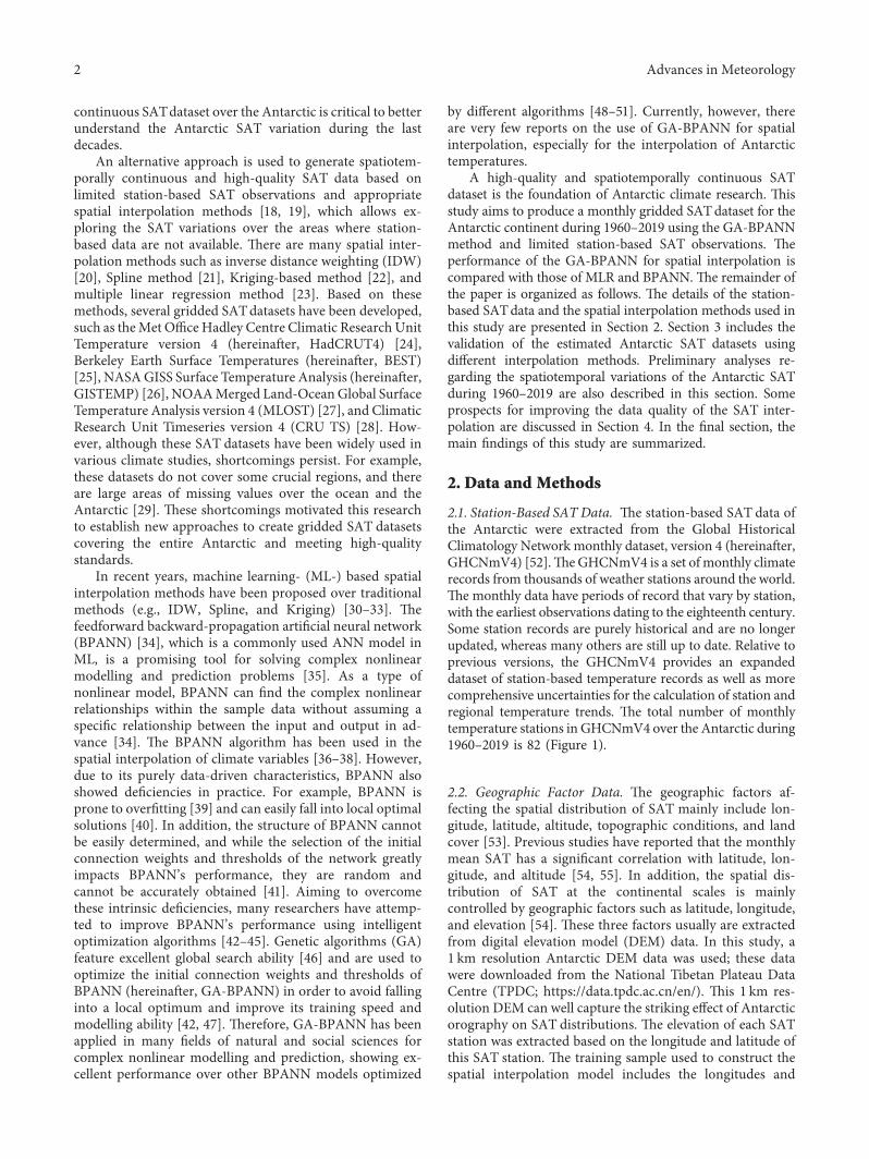


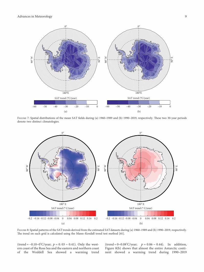


![Data Book AGA 60 D · Aluminium for version AGA 076 - AGA 106 [8] With gasket in NBR only for version single phase AGA 106 . CENTRIFUGAL PUMPS AGA CONSTRUCTIONS 60Hz 301 EBARA Pumps](https://static.documents.pub/doc/80x56/5e694725e04bf5741b5a9b0e/data-book-aga-60-d-aluminium-for-version-aga-076-aga-106-8-with-gasket-in-nbr.jpg)


![AGA BlueBookFall2010[1]](https://static.documents.pub/doc/80x56/577d1d371a28ab4e1e8bd79d/aga-bluebookfall20101.jpg)


