Agency-Based Asset Pricing * Lixin Huang Georgia State University §§§ First Draft: November 8, 2003 This Draft: October 15, 2011 Abstract We study an infinite-horizon Lucas tree model where a manager is hired to tend to the trees and is compensated with a fraction of the trees’ output. The manager trades shares with investors and makes an effort that determines the distribution of the output. When the manager is less risk-averse than the investors, managerial trading smoothes output and results in a less volatile stock price and a lower risk premium; when the manager is more risk-averse, output and the stock price become more volatile and the risk premium is higher. Trading between the manager and investors acts as an indirect renegotiation mechanism that dynamically modulates the manager’s incentives, and in the meantime, allocates risk and return, but its effectiveness is limited when the market consists of dispersed small investors. * We would like to thank Debbie Lucas, Randall Morck, Larry Samuelson, Feng Gao and seminar participants at Columbia University, the IMF, and Georgia State University for helpful comments and suggestions. § School of Management, Yale University, New Haven, CT 06520-8200. E-mail: [email protected]. §§ Tsinghua University, School of Economics and Management, Beijing 100084, China. E-mail: [email protected]. §§§ J. Mack Robinson School of Business, Georgia State University, Atlanta, GA 30303. Email: [email protected]. Gary B. Gorton Yale University and NBER § Ping He Tsinghua University §§
Transcript
Agency-Based Asset Pricing*
Lixin Huang
Georgia State University§§§
First Draft: November 8, 2003
This Draft: October 15, 2011
Abstract
We study an infinite-horizon Lucas tree model where a manager is hired to tend to the trees and is compensated with a fraction of the trees’ output. The manager trades shares with investors and makes an effort that determines the distribution of the output. When the manager is less risk-averse than the investors, managerial trading smoothes output and results in a less volatile stock price and a lower risk premium; when the manager is more risk-averse, output and the stock price become more volatile and the risk premium is higher. Trading between the manager and investors acts as an indirect renegotiation mechanism that dynamically modulates the manager’s incentives, and in the meantime, allocates risk and return, but its effectiveness is limited when the market consists of dispersed small investors.
* We would like to thank Debbie Lucas, Randall Morck, Larry Samuelson, Feng Gao and seminar participants at Columbia University, the IMF, and Georgia State University for helpful comments and suggestions. § School of Management, Yale University, New Haven, CT 06520-8200. E-mail: [email protected]. §§ Tsinghua University, School of Economics and Management, Beijing 100084, China. E-mail: [email protected]. §§§ J. Mack Robinson School of Business, Georgia State University, Atlanta, GA 30303. Email: [email protected].
Gary B. Gorton Yale University and NBER§
Ping He Tsinghua University §§
2
1. Introduction
The canonical asset pricing model views corporate cash flows as exogenous and focuses on identifying a stochastic discount factor or pricing kernel to price the assumed cash flows. On the contrary, the standard corporate finance model views the pricing kernel as exogenous and emphasizes the impact of managerial incentives on corporate cash flows to be priced by the given pricing kernel. Overall then, in the paradigm of financial economics there is a separation between asset pricing and corporate finance.
In this paper we incorporate a standard agency problem into a classical asset pricing model to simultaneously endogenize the pricing kernel and the cash flows. Specifically, we analyze an infinite-horizon Lucas tree model where a manager needs to be hired to tend to the trees and is compensated with a fraction of the trees’ output. The manager trades shares with investors and makes an effort that determines the output. The stock price in this model plays two critical roles: in addition to the usual risk-sharing mechanism, it also acts as a monitoring mechanism that induces the manager to make an effort. The interaction between these two roles results in the reciprocal impact of the pricing kernel and cash flows.
The necessity of explicitly modeling the manager’s trading decisions and effort choices poses challenges to the analysis. Since the manager’s effort determines cash flows, he has to be modeled as a “big” corporate player. But, the manager’s effort depends on his shareholding, so the manager’s trading decisions have an impact on the share price and he also has to be modeled as a “big” trader––a non-price-taker–– in the stock market. We construct a dynamic model in which the manager controls cash flows and trades as a monopolist with a continuum of small competitive investors. For the equilibrium concept, the literature adopts state-dependent Perfect Public Equilibria (PPE) (see Phelan and Stacchetti (2001) for the example of a big government and a continuum of individuals and Atkeson (1991) for the example of two big agents as extensions of Abreu, Pearce, and Stacchetti (1986, 1990)). In a PPE, the recursive state-dependent value correspondences characterize the equilibrium value sets. However, working with value correspondences is difficult, even numerically, and in addition, equilibrium selection is a problem. We propose a Strong Markov Perfect Public Equilibrium (SMPPE) that allows us to work with value functions instead of value correspondences. This generalizes the application of dynamic programming to broader economic settings beyond the traditional competitive market environment. Though more restrictive, SMPPE facilitates our understanding of the model and eases numerical analysis.
Our analysis shows that managerial trading has a large impact on the stock price. This impact depends on the relative risk tolerance between the manager and the investors. When the manager is more risk-averse than the investors, output and the stock price become more volatile and the risk premium is higher; when the manager is less risk-averse than the investors, managerial trading smoothes output and results in a less volatile stock price and a lower risk premium. In addition to its risk-sharing function, trading between the manager and investors also acts as an indirect renegotiation mechanism that dynamically modulates the manager’s incentives. However, when the market consists of small competitive investors, the effectiveness of the incentive function is limited. The
3
conventional wisdom posits that managerial trading leads to an unraveling of incentives, but we find that the opposite can also be true, especially when the manager is less risk-averse than the investors.
Although the literature on managerial compensation is voluminous (see surveys by Abowd and Kaplan (1999), Murphy (1999, 2002), Bebchuk and Fried (2004), Holmström (2005), Core, Guay, and Thomas (2005), among many others), the general understanding of the relation between managerial compensation and firm performance is still very limited, and there are different opinions about managerial pay performance sensitivity. The nub of the issue is the tension between risk-sharing and incentive provision. Having the manager own all of the equity would solve the agency problem, but would also expose the manager to too much risk. While stock compensation can be used to alleviate moral hazard by aligning the interests of firm managers and investors, its effectiveness is limited by the need of risk-sharing between these agents in the economy. For example, in response to Jensen and Murphy’s (1990) finding of low pay performance sensitivity estimate, Garen (1994) and Haubrich (1994) show that a manager’s risk concern has an impact on the effectiveness of the stock compensation. When a manager’s shareholding changes, his incentive also changes, resulting in changes in cash flows. The stock price reflects the changes in cash flows, and in the meantime, affects the manager’s trading decisions that impact cash flows. In this sense, the pricing kernel and cash flows are simultaneously and inseparably determined. Most of the papers in the literature study static models that do not consider the interaction between the pricing kernel and cash flows, let alone the dynamics in a multi-period framework. The main contribution of this paper is to provide a general dynamic modeling framework that enables us to comprehensively analyze the effect of managerial compensation on asset pricing.
A recent paper closely related to ours is DeMarzo and Urosevic (2006), who study the trading behavior of a large shareholder in a similar model setup.1 Despite the similarity in the theoretical structure, our paper significantly differs from DeMarzo and Urosevic (2006) in several aspects. They assume that agents have CARA utilities and shares of the firm can only be traded at discrete times in a continuous-time setting. As a result of these assumptions, the large shareholder’s trading decision and the share price do not depend on the realized cash flows. They find that managerial holding gradually converges toward the competitive allocation in such a way that everything is time deterministic given the initial ownership. We study a more general case without restrictions on preferences and trading times.2 Our results demonstrate richer dynamics that are not time deterministic. The manager’s trading direction depends on the realized cash flows as well as on the relative risk attitude of the manager and the investors. We show that the interaction of risk-sharing and moral hazard can make the stock price more or less volatile depending on whether the manager is more or less risk-averse than the investors. Finally, we formally define Strong Markov Perfect Public Equilibrium and prove the existence of such an equilibrium.
1 Except for the difference in terminology, there is no theoretical difference in calling an agent a “manager” as in our paper or a “large shareholder” as in DeMarzo and Urosevic (2006). Empirically a firm manager has more direct controls over the firm’s operations but less trading flexibility than a large shareholder. 2 Although we use CRRA utility functions for the one-period model in Section 3, the Strong Markov Perfect Public Equilibrium we characterize in Section 4 applies to any utility functions.
4
Our paper is a generalization and extension of the literature that studies the effects of agency problems on asset pricing equilibrium. Admati, Pfleiderer, and Zechner (1994) study a model that is a static version of DeMarzo and Urosevic (2006), and rely on CARA utility and certainty equivalence to analyze the tension between risk-sharing and costly monitoring. Kihlstrom and Matthews (1990) and Magill and Quinzii (2002) also study the static asset market equilibrium based on the assumptions that entrepreneurs cannot control the market price of risk and that certain spanning conditions hold. Holmström and Tirole (2001) focus on asset pricing implications of firms’ inability to contractually pledge future income to external investors. In addition to these static models, there are dynamic models that attempt to integrate corporate agency problems into asset pricing. Dow, Gorton and Krishnamurthy (2005) incorporate Jensen’s free cash flow theory into a dynamic asset pricing model, but they do not consider risk sharing between the manager and investors. Albuquerque and Wang (2008) study the asset pricing implications of different levels of investor protection, and examine the effects on Tobin’s q, risk premia, and volatility. He and Krishnamurthy (2008) are concerned with the effect of bank capital on the pricing kernel when intermediaries are the marginal investors. Sung and Wan (2009) show that it is optimal for the principal to forbid the agent to trade the firm’s equity in the stock market. Unlike our paper, none of these papers models the manager as both a corporate decision maker who affects cash flows and a monopolist trader who affects the stock price.
In most part of the paper, we consider dispersed outside investors interacting with the manager through the stock market. This is different from papers on optimal long-term managerial contracts, such as Holmström and Milgrom (1987), Spear and Srivastava (1987), and Ou-Yang (2005). When outside investors are dispersed and behave competitively, they act independently based on their beliefs about the manager’s trading decisions and effort choices. The equity price consistently reflects these beliefs and induces the manager to behave as expected. The initial managerial shareholding represents the initial contract between the manager and the investors. Trading between the manager and outside investors can be viewed as an indirect renegotiation mechanism that dynamically modulates the manager’s incentive and allocates risk and return. In an extension, we examine the case where dispersed investors are replaced by a single blockholder. We show that the blockholder can monitor the manager more effectively.
We proceed as follows. In Section 2, we set up the model. To build understanding of the interaction between risk-sharing and incentive provision, we first study a simplified one-period case in Section 3. We define the equilibrium concept of SMPPE for the full-blown infinite-horizon model in Section 4. In addition, we characterize the equilibrium, prove its existence, and provide numerical examples to illustrate the equilibrium. In Section 5, we study the case of a single blockholder. We conclude in Section 6.
2. Model Set-up
We introduce the managerial moral hazard problem into the classic Lucas (1978) asset pricing model. Specifically there are two types of agents in the economy, an entrepreneur and a measure-one continuum of investors. The assets in the economy are Lucas trees
5
that need to be watered properly to bear fruit. The investors own these trees, but do not possess the skill to water them. The entrepreneur knows how to water the trees. Therefore, the investors hire the entrepreneur as the manager to take care of the trees. We assume that the investors are homogeneous and only consider a representative investor’s dynamic decisions.
At the beginning of each period t, the manager chooses an effort level et, which is unobservable by the investors and which determines the trees’ output. The output is a random variable defined on a support +⊆= RyyY ],[ that is invariant to the effort level et. However, the distribution of yt over the support Y depends on the manager’s effort et. Specifically, conditional on the effort level, yt has a distribution density function f(yt|et). We assume that the density function f(yt|et) satisfies the monotone likelihood ratio condition:
Assumption 1: The density function f(y|e) satisfies the monotone likelihood ratio condition (MLRC); that is, for e > e’, f(y|e)/f(y|e’) is increasing in y.
The MLRC implies that the manager’s effort is desirable in the sense of increasing productivity. When the manager makes a higher effort, the level of output is more likely to be high.3 Output is perishable. After yt is realized in period t, it is distributed as dividends. The manager and the investors can either consume the dividends or trade for shares in the stock market. The fraction of shares that the manager owns before trade in period t is denoted as αt. The manager trades Δαt and owns αt+1 = αt + Δαt at the beginning of period t + 1. The representative investor’s shareholding before trade in period t is denoted as αit, which is equal to 1 – αt. After trading Δαit the investor owns αit+1 = αit + Δαit shares at the beginning of period t + 1. The price pt is formed to clear the market: αt+1 + αit+1 = 1. After trading in the stock market, the next period starts. To summarize, the sequence of events in each period t is as follows:
1. The manager, with an equity share of ]1 ,0[∈tα , chooses an effort level et;
2. Nature chooses output yt according to the density function f(yt|et); 3. All the output is distributed as dividends; the manager receives αtyt, and the
representative investor receives αityt; 4. Trading in the stock market begins. After trading at price pt, the manager ends up
with αt+1 shares of the equity, and the investor ends up with αit+1 shares of the equity;
5. Consumption occurs and the next period starts.
The manager’s period-t consumption is given by ( ) tttttmt pyc ααα −−= +1 , and the investor’s consumption is given by ( ) titittitit pyc ααα −−= +1 . We assume that the
manager’s lifetime expected utility is [ ]⎥⎦
⎤⎢⎣
⎡−∑
∞
=0)()(
ttmt
t egcuE δ and the representative
3 The monotone likelihood ratio condition implies first-order stochastic dominance, and thereby second-order stochastic dominance as well.
6
investor’s lifetime expected utility is ⎥⎦
⎤⎢⎣
⎡∑∞
=0)(
tit
t cvE δ , where u(.) and v(.) are the
consumption utility functions, g(.) is the effort cost function, and )1 ,0(∈δ is the discount factor. We assume that u(.) and v(.) are increasing and concave; g(.) is increasing and convex; that is, uc > 0, ucc ≤ 0, vc > 0, vcc ≤ 0, ge > 0, and gee ≥ 0. We impose short sale constraints on both the manager and the investors. Therefore,
]1 ,0[∈tα in any period t.
3. One-Period Model
To illustrate the main idea of the paper, we first study a one-period (two-date) model with managerial trading. Specifically, at date 0, the manager owns α0 portion of the total equity and the investor owns a fraction 1 – α0 of the firm’s shares. The firm’s output is y0, which is perishable and distributed as dividends. Upon receiving the dividends, the manager and the investor start trading in the stock market, after which the manager chooses an effort level e, which is unobservable by the investors. Conditional on this effort level, the output at date 1, y1, follows a distribution density function f(y1|e) defined on the support +⊆= RyyY ],[ . The support Y is invariant to the effort level e; therefore, y1 is an imperfect signal of the effort choice, e.
Suppose that the manager owns a fraction α1 of the total equity after trading. At date 0, the manager’s consumption is ( )pycm 01000 ααα −−= , and the investor’s consumption is ( )pyci 01000 )1( ααα −+−= . At date 1, the manager’s consumption is 111 ycm α= , and the representative investor’s consumption is 111 )1( yci α−= .
The manager is risk averse over consumption, and suffers a disutility from making effort e. The manager’s lifetime expected utility is )(]|)([)( 10 egecuEcu mm −+ δ . The representative investor’s lifetime expected utility is ]|)([)( 10 ecvEcv ii δ+ . Again we impose short sale constraints on both the manager and investors.
3.1 Equilibrium Definition
The manager’s strategy is to choose the trading amount, Δα = α1 – α0 based on his shareholding, α0, and output, y0, at date 0, and then to choose the effort level, e, based on his shareholding α1. As for the representative investor, he trades competitively as a price-taker, and his strategy can be written as )(1 piα .
Given α1, the manager’s optimal effort choice is the solution to the problem below:
[ ]...
)(|)(max
111
1
yctsegecuE
m
me
αδ
≤−
(1)
7
We will analyze a sequential equilibrium for the game, in which the manager and the investors rationally expect the effort choice when they trade. Let us denote the solution to (1) as e*(α1). Since the manager is a monopolist trader, we use p*(α1) to denote the equilibrium pricing function of the trading equilibrium. The manager chooses α1 by solving the following optimization problem:
[ ]
.)()(
..
))(()(|)()(max
111
1*
01000
1*
1*
101
ycpyc
ts
egecuEcu
m
m
mm
ααααα
ααδα
≤−−≤
−+
(2)
Given the manager’s effort choice and trading strategy, for any price level, p, the representative investor trades competitively and chooses αi1 to maximize his utility:
[ ]
.)(
..
)(|)()(max
111
01000
1*
101
ycpyc
ts
ecvEcv
ii
iiii
iii
αααα
αδα
≤−−≤
+ (3)
We use *1α to denote the manager’s optimal trading strategy, associated with (2), and use
),( 1*1 pi αα to denote the investor’s trading strategy, associated with (3). In equilibrium,
the market clears and p* is such that 11*
1*1 1))(,( αααα −=pi .
Definition 1 (Sequential Equilibrium) A sequential equilibrium satisfies the following conditions:
1. The manager has no incentive to deviate, that is, for any α1, )( 1* αe is the solution
to (1); and given )( 1* αe and p*(α1), *
1α is the solution to (2). 2. For any choice of 1α made by the manager, the representative investor rationally
anticipates )( 1* αe , and has no incentive to deviate from )(*
1 piα for any given price p.
3. For any α1 chosen by the manager, p*(α1) clears the market: 11
*1
*1 1))(,( αααα −=pi .
Notice that the above conditions imply that, even for an off-equilibrium path choice of *11 αα ≠ , we still require the optimality of the manager’s effort choice and the
representative investor’s trading strategy to clear the market.
It is easy to check that a sequential equilibrium outcome is a triplet )(),(, 1*
1**
1 ααα pe , which can be characterized by the following conditions:
1. The manager’s optimal effort choice:
,0))(())(|()( 1*
11*
11 =−∫ αα egdyeyfcu ee em (4)
where 111 ycm α= , for any ]1 ,0[1 ∈α .
8
2. The manager’s optimal trading strategy:
[ ] )),(()(|)()(maxarg 1*
1*
10]1,0[*1 1
ααδα α egecuEcu mm −+= ∈ (5)
where . and )()( 1111*
01000 ycpyc mm ααααα =−−=
3. The investor’s optimal trading strategy:
[ ] ,0)(|)(/)()( 1*
0111* =+− αδα ecvcvyEp icic for any ]1 ,0[1 ∈α , (6)
where 1111*
01000 )1( and ,)()()1( ycpyc ii ααααα −=−+−= .
Notice in (4), the optimality of e* applies to the manager’s trading decision of α1, regardless of on or off the equilibrium path, and this is a critical condition for a sequential equilibrium. Similarly, the first order condition in (6) also holds for any on- or off-equilibrium trading decision, α1, made by the manager, while imposing the market clearing condition: 11
*1
*1 1))(,( αααα −=pi .
3.2 Managerial Trading without the Agency Problem
For tractability, we assume the following for the rest of this section:
.1
)( ,1
)(11
i
ii
m
mm
im ccv
ccu
γγ
γγ
−=
−=
−−
Using the first order condition for (5) and the Envelope Theorem, we can show that, the manager’s portfolio choice )1 ,0(1 ∈α satisfies the following condition:
.0)](|)([)(])()([ 1*
110*
011* =+−+− αδααα α ecuyEcupp mcmc (7)
Comparing (7) with (6), the representative investor’s portfolio choice, we can see that the manager’s marginal cost of trading consists of two parts: the stock price, p*, and the price impact, Δp* = *
01* )()( αα ααα pp −=Δ , due to the fact that the manager is not a price-
taker. Let us denote the manager’s private valuation of the equity as pm. We have:
[ ].)(|)(/)()()( 1*
011*
011* αδααα α ecucuyEppp mcmcm =−+≡ (8)
Both the manager and the representative investor would like to trade to smooth consumption based on the realization of y0, and depending on the level of risk aversion, the less risk-averse agent will provide insurance to the more risk-averse one. However, trading will affect the manager’s incentive to exert effort. The incentive concern will feedback to the stock price, and the manager’s trading decision should fully incorporate this feedback effect.
The effect of managerial trading on the stock price comes from two sources: the manager trades as a monopolist and trading changes his effort choice. To distinguish between these two effects, we first focus on the monopolist effect by shutting down the channel of the agency problem and assuming that effort is an exogenously given constant.
9
Proposition 1 (Trading without the Agency Problem) Without the agency problem (assuming managerial effort, e, is exogenously given), there exists a unique output level y*(α0, e) ),( yy∈ at which the manager does not trade, and we have: (i) If γm > γi, the manager buys (sells) shares when y0 >(<) y*(α0, e); (ii) If γm < γi, the manager sells (buys) shares when y0 >(<) y*(α0, e). In addition, the manager trades less aggressively– buys or sells fewer shares– than in the case where he is a price taker.
Proof: See Appendix A.
Intuitively, agents want to smooth consumption. When the manager is more risk-averse than the investors (γm > γi), the manager buys shares when the output is high and sells shares when the output is low. In this case, the investors provide insurance to the manager. When the manager is less risk-averse than the investors (γm < γi), it is exactly the opposite. Since the manager is a monopolist, he drives up (down) the price when he buys (sells) shares. The consideration of the price impact prevents him from trading as much as in the case where he is a price-taker, in which case, his trading does not have any impact on the price.
3.3 The Effect of the Agency Problem
The manager’s effort choice equalizes the marginal cost to the marginal benefit, which is the additional utility due to the output distribution shifted toward the high end. With the assumed CRRA utility, the marginal value of an additional share, y1uc(cm1), may increase or decrease with the level of output, depending on the risk aversion coefficient, γm. This dependency determines how the manager’s effort changes with his shareholding, α1.
Lemma 1 (The Manager’s Effort Decision) If γm < 1 (> 1), then the optimal effort level, e, is increasing (decreasing) in the manager’s shareholding, α1.
Proof: See Appendix A.
Lemma 1 shows that only under certain conditions is the manager’s effort increasing in his shareholding. Since the logic of managerial ownership as an incentive mechanism is built upon the assumption that managerial effort is increasing in the manager’s shareholding, we assume γm < 1 for the rest of this section to guarantee that this logic holds. By doing so, we focus on the tension between incentive provision and risk sharing.4
With the agency problem, the manager’s trading behavior will be different. The key driving force is the sensitivity of the stock price to the manager’s shareholding. With the assumption of γm < 1, the manager’s effort choice will increase with his shareholding. This yields the cash flow effect. The change of cash flows is going to affect the investor’s trading decisions and consequently affect the stock price. If the manager’s price impact is enhanced by his effort choice, then the interaction can feedback to reduce the manager’s
4 If the manager has other income in addition to dividend income, then it is possible that his effort is increasing in his shareholding even if γm >1. In an earlier version, we analyzed such cases. To focus the discussion we omit these cases here.
10
trading intensity. On the other hand, if the manager’s price impact is dampened by his effort choice, then the manager is going to trade more aggressively. The following proposition characterizes these interactions.
Proposition 2 (Trading with the Agency Problem) With the agency problem, (i) there exists a unique no-trade output level y*(α0, e*(α0)) ),( yy∈ that coincides with the no-trade point in the absence of the agency problem with the given exogenous managerial effort equal to e*(α0); (ii) if γm > γi, the manager buys (sells) shares when y0 >(<) y*(α0, e*(α0)); if γm < γi, the manager sells (buys) shares when y0 >(<) y*(α0, e*(α0)); and (iii) when γi > (<) 1, the manager will trade more (less) aggressively than in the case without the agency problem.
Proof: See Appendix A.
Intuitively, the representative investor’s marginal value of holding an additional share is equal to yvc(ci1), which increases in y when γi < 1 and decreases in y when γi > 1. Under the assumption that γm < 1, the manager’s effort is increasing in his shareholding. When the manager buys shares, he makes a greater effort that results in more likely high output levels and less likely low output levels. The investor takes this shift in the output distribution into consideration and adjusts the demand for the stock accordingly. When γi < 1, the investor’s marginal value of an additional share increases with the manager’s share holding. The resulting price pressure due to the agency problem feeds back to the manager’s trading decision and induces him to trade less aggressively. In the case of γi > 1, the effect of the agency problem on the stock price dampens the manager’s monopolistic trading impact, and makes the manager trade more aggressively.
With the agency problem, the effort choice ensuing from the manager’s trading decisions endogenously determines productivity in the model economy. This has rich implications for economic fluctuations.
Proposition 3 (Agency Problem and Economic Fluctuations) (i) If γm < γi, then managerial trading will generate mean reversion in output; (ii) If γm > γi, then managerial trading will amplify the output fluctuations.
Proof: See Appendix A.
The intuition behind Proposition 3 is straightforward. If the manager is less risk-averse than the investors, Proposition 2 tells us that the manager sells shares when the output is high and buys shares when the output is low. According to Lemma 1, managerial effort in the second period is increasing in managerial shareholding with γm < 1. Therefore, high output at date 0 tends to result in low productivity at date 1 and low output at date 0 tends to result in high productivity at date 1. In other words, the agency problem can generate an endogenous mean-reverting business cycle. Contrarily, when the manager is more risk-averse than the investors, he buys (sells) shares when the date-0 output is high (low) and exerts a greater (lesser) effort at date 1. As a result, the joint force between risk-sharing and managerial incentive is likely to amplify output shocks.
11
3.4 Asset Pricing Implications
Suppose the small investors can trade a bond in zero net supply.5 The price of the risk free zero-coupon bond is:
.|)()(
)(0
11 ⎥
⎦
⎤⎢⎣
⎡≡ e
cvcv
Ebic
icδα (9)
The realized equity premium given output y1 can be written as:
)(1
)(),(
11*
111 αα
αbp
yy −=Π , (10)
and the ex ante expected equity premium can be written as:
[ ]. |),()( 111 eyE ααπ Π= (11)
Proposition 4 (Equity Premium) Without the agency problem, the equity premium decreases in α1. With the agency problem, the equity premium can either increase or decrease in α1
Proof: See Appendix A.
To understand Proposition 4, we first have a look at the effect of trading on the stock return. We can write out the first order approximations for the equity price and the output density function, as follows:
).)(())(|())(|())(|(
),()()(
010*
0*
10*
11*
1
01*
0*
1*
αααααα
αααα
α
α
−+≈
−+≈
eeyfeyfeyf
ppp
e
(12)
The realized equity return can be written as:
.)()(
),(01
*0
*1
11 αααα
α −+≈
ppyyr (13)
Given α0, the expected equity return conditional on the date-0 output, y0, can be written as:
.)()(
))(()(|()](|[]|),([
01*
0*
10*10
*0
*110
*1
111 ααα
ααααααα
α
α
−+
−+≈ ∫
pp
dyeeyfyeyEyrE
eY (14)
From (14), we can see that trading affects the equity return in two ways: (i) the monopolistic price effect (denominator effect), which corresponds to the first approximation in (12); and (ii) the cash flow effect (numerator effect) due to the extra effort expended by the manager, which corresponds to the second approximation in (12).
5 Since investors are homogeneous, there is no bond trading in equilibrium. Further, since the manager is a monopolist and sets the equity price, we do not consider the manager’s participation in the bond market. Allowing the manager to participate in the bond market involves a lot of complicated issues; for example, there is the question of how to enforce debt repayment; and the question of what happens if the borrower becomes insolvent, etc.
12
Without the agency problem, the cash flow effect does not exist; therefore, the effect of managerial trading on the stock return is a pure price effect: the more shares owned by the manager, the higher the price, and the lower the stock return. With the agency problem, the interaction of the monopolistic price effect and the cash flow effect depends on the risk preferences of the manager and the investors. The assumption of γm < 1 guarantees that the manager’s effort is increasing in α1, that is, 0* >αe ; hence the cash flow effect is positive. The overall effect of trading on the stock return depends on the relative magnitude of the two effects. If the cash flow effect dominates the price effect, then the stock return increases in α1; if the price effect dominates the cash flow effect, then the stock return decreases in α1.
Similar to the effect on the stock return, the effect of α1 on the equity premium also comes through two channels: first, the direct effect on asset prices, p*(α1) and b(α1); second, the indirect cash flow effect on the distribution of y1. The proof in Appendix A shows that the direct price effect is captured by ),( 11 yααΠ , and the indirect cash flow effect is captured by ).|(/)|(),( 1111 eyfeyfey eααΠ The correlations of these two effects with the investor’s marginal utility determine the effect of managerial trading on the equity premium. Without the agency problem, the second channel for the cash flow effect is shut down and the price effect solely determines that the equity premium decreases in α1. With the agency problem, there is an additional positive cash flow effect on the equity premium. Specifically, a higher α1 is going to increase the likelihood of high output states, where the investor’s marginal utility is low. The negative correlation between the investor’s marginal utility and the cash flow effect results in a higher risk premium. Again, the net effect of managerial trading on the equity premium depends on the relative magnitude of the conflicting price effect and cash flow effect.
4. Model with Infinite Horizon
Our analysis above demonstrates the tension between the manager’s trading decision and his effort choice, as well as the effect of this tension on the asset price. The main purpose of this paper is to analyze a dynamic infinite-horizon model with this tension. Similar to Section 3, we will study sequential equilibria, in which the strategies of both the manager and the representative investor depend only on public information. This type of equilibrium is called Perfect Public Equilibrium (PPE) (see Fudenberg, Levine, and Maskin (1994)).
In period t, the manager first decides on his effort choice, et, based on his stock ownership, αt. Then, output, yt, is realized and the manager trades shares with the investor. The manager chooses the number of shares to trade, ]1 ,[ ttt ααα −−∈Δ . The representative investor is a price taker, submitting a demand function Δαit(pt). The equilibrium price tp clears the market such that 0)( =Δ+Δ titt pαα . The public history is denoted as 1
010 )(,,,, −=+ ΔΔ∪= t
it pyph ττττττ αααα . We denote the economy at t =
0 by Φ(α0) because the manager’s shareholding, α0, is the only state variable. The
13
investor’s strategy σi can be written as ∞=+Δ 01 ),,( ttt
tit pyhα ; the manager’s strategy σm
can be written as ∞=Δ 0),(),( tt
tt
tt yhhe α . A strategy profile for the economy Φ(α0) is a
pair of strategies σ = (σm, σi), one for the manager and one for the representative investor.
Phelan and Stacchetti (2001) use an auxiliary competitive equilibrium to characterize the Perfect Public Equilibrium. We take the same approach and construct an auxiliary competitive equilibrium by assuming that the manager adopts an exogenous strategy mσ . With the manager’s strategy exogenously given, we denote the economy at t = 0 by Φ(α0|σm). As a first step toward the solution to the dynamic model, we solve for the representative investor’s equilibrium strategy in such an economy.
4.1 An Auxiliary Competitive Equilibrium
As in Section 3, when the manager’s strategy is given, the distribution of output is also exogenously given and the density function is determined by:
)).(|()|(ˆ ttt
tt heyfhyf = (15)
In this subsection, all the expressions, including the expression in (15), are conditional on the manager’s given strategy σm, and to simplify the notation, we omit σm in all expressions. The representative investor’s optimization problem is:
⎥⎦
⎤⎢⎣
⎡∑∞
=0)(
tit
t cvE δ (16)
,)(.. 1 titittitit pycts ααα −−≤ +
where consumption cit consists of the dividends paid on the equity shares held by the investor plus the income from shares sold. The competitive equilibrium of the economy Φ(α0|σm) is a sequence of stock prices p = ∞
=0 ttp and a sequence of consumption and share allocations ∞
=+ 01 ),(),,( ttt
ittt
it yhyhc α , such that:
1. Given ∞=0 ttp , ∞
=+ 01 ),(),,( ttt
ittt
it yhyhc α maximizes [ ])(0∑∞
=t itt cvE δ .
2. Δαit = αit+1 – αit = – Δαt, for any t.
The logic of this equilibrium is explained in Phelan and Stacchetti (2001). In brief, when there is a continuum of players, individual agents, investors in our case, cannot change the outcome of the game by deviating since their deviation is not observable. Phelan and Stacchetti (2001) show that an implication of this logic is that agents’ incentive constraints are their Euler conditions in equilibrium. Moreover, as we will show, the auxiliary competitive equilibrium of this economy is equivalent to a corresponding static one-period economy defined below. This equivalence result is the key to define our equilibrium concept in the next subsection.
Define
)].()[( 1111 ++++ +≡ itcttt cvpyEM (17)
14
This variable represents the investor’s marginal expected lifetime utility for an additional share of the stock he holds in period t + 1 and summarizes all the information the investor needs to make consumption and investment decisions at time t. Suppose we have solved the auxiliary competitive equilibrium for the economy Φ(α0|σm). We can calculate the value of Mt+1 every period. Let us construct a one-period economy where the investors have initial shareholdings of αit = 1 – αt and Mt+1 is taken as exogenously given. Since the manager’s trading strategy and effort choice are now exogenously given, the investor in this one-period economy chooses the shareholding after trading in period t: αit+1. The investor’s augmented utility function over consumption and end-of-period shareholding is v(cit) + δMt+1αit+1. The competitive equilibrium of this static one-period economy consists of a price pt and a pair (αit+1, cit) such that the following two conditions are satisfied: (i) given pt, αit+1 maximizes v(cit) + δMt+1αit+1; (ii) αit+1 = 1 – αt+1.
Let CE(αit, Mt+1) denote the set of competitive equilibrium allocations (cit, αit+1) of this static one-period economy. In order to establish Perfect Public Equilibrium with endogenous managerial strategies, we will need the boundedness of Mt to satisfy the transversality condition. As shown by Phelan and Stacchetti (2001), the transversality condition holds if we impose boundary conditions on the investor’s marginal utility. Further, there is an equivalence between the auxiliary competitive equilibrium for the infinite-horizon economy and the competitive equilibrium for the static one-period economy.
Proposition 5 (Equivalence to Static One-period Equilibrium) If there exist cc vv <<0 such that ∞<<<< ccc vcvv )(0 , then Mt is bounded from above in a competitive equilibrium of the economy Φ(α0|σm). For ∞
=+ 0*
1* , tititc α to be a competitive allocation of
the economy Φ(α0|σm), a necessary and sufficient condition is that, for all t and ht, ),( *
1*
+ititc α is the static one-period equilibrium outcome, that is, ),(),( *
1**
1*
++ ∈ tititit MCEc αα .
Proof: See Appendix A.
With the satisfaction of the transversality condition and the existence of the auxiliary competitive equilibrium, we can represent the infinite-horizon dynamic problem with recursive functions, as shown below.
4.2 Strong Markov Perfect Public Equilibria
We analyzed the auxiliary equilibrium in the previous subsection by taking the manager’s strategy, σm, as exogenously given. Our purpose in this subsection is to characterize the dynamic equilibrium in which both the manager’s decisions and the investor’s decisions are endogenized. For a given strategy profile σ = (σm, σi), we define the manager’s expected lifetime utility as:
,)]()([][0
⎥⎦
⎤⎢⎣
⎡−= ∑
∞
=ttmt
t egcuEU δσ (18)
15
and the investor’s expected lifetime utility as:
.)(][0
⎥⎦
⎤⎢⎣
⎡= ∑
∞
=tit
t cvEV δσ (19)
The recursive formalization of the dynamic equilibrium involves not only the payoffs to the manager and the investor but also the marginal value of shares for the investors. For any strategy profile σ = (σm, σi), we define the marginal value of shares for the investors at the very beginning of the game as:
)].()[(][ 000 ic cvpyEM +=σ (20)
The role of M[σ] is to enable us to establish the equivalence relation between a dynamic equilibrium and a one-period static equilibrium.
Definition 2 (Perfect Public Equilibrium) A strategy profile σ = (σm, σi) is a Perfect Public Equilibrium (PPE) for the economy Φ(α0) if for any τ ≥ 0, and history ττ Hh ∈ , the following conditions are satisfied:
1. Given the investor’s strategy σiτ, the manager has no incentive to deviate, that is, U[(σmτ, σiτ)] ≥ U[(σ′mτ , σiτ)] for any σ′mτ ≠ σmτ , where (σmτ, σiτ) = (σm, σi)t ≥ τ is the equilibrium strategy profile σ = (σm, σi) starting from t = τ ; 2. ∞
=+− τα titt c ,1 1 is an auxiliary competitive equilibrium allocation of the economy Φ(ατ|σmτ) corresponding to the manager’s shareholding ατ and the exogenously given strategy σmτ= (σm)t ≥ τ.
The definition of the PPE imposes two conditions. The first condition requires that the manager’s continuation strategies be best responses of the investor’s continuation strategies after any history hτ. The second condition states the optimality of the investor’s decision in an auxiliary competitive equilibrium we analyzed in Section 4.1. In a PPE, the continuation payoffs have to correspond to PPE profiles, so the lifetime expected payoffs can be factored into current payoffs and continuation payoffs. Appendix B demonstrates the recursive factorization of the defined PPE. Correspondingly, the PPE utility values, U[σ], V[σ] and M[σ], defined upon the strategy profile σ = (σm, σi) can be replaced with simplified state-dependent value correspondences. In the context of our model, the state variable is the distribution of shareholdings across investors. When all dispersed homogeneous investors hold the same fraction of equity, the distribution of shareholdings is degenerated to a single variable—the manager’s shareholding, α. The value correspondences (U(α), V(α), M(α)), defined upon α. can be formally written as:
.)(economy for the PPE a is |])[]),[],[())(),(),(( ασσσσααα Φ= MVUMVU (21)
The recursive formalization of the PPE only delivers value correspondences that depend on α , but the strategies of the manager and the investor still depend on the history. In seeking tractability, we restrict attention to strategies where the manager’s and the investor’s decisions only depend on α. These strategies, which condition on the realization of a state variable, are known as Markovian strategies. A Markov Perfect Public Equilibrium (MPPE) is a Perfect Public Equilibrium in which both the manager
16
and the investor play time-invariant Markovian strategies (see Fudenberg and Tirole (1991) for the definition of Markov Perfect Euqilibrium (MPE)).
Since MPPEs do not impose any restrictions on what happens off the equilibrium path, there are many different MPPEs depending on the off-equilibrium beliefs. For example, given α, after a certain output y is realized, on the equilibrium path the manager will trade to hold α′ for the next period, and this can be implemented by specifying an off-equilibrium continuation PPE that punishes the manager with a very low payoff if he deviates and holds α′′ ≠ α′. The off-equilibrium continuation PPE can be any PPE; that is, it can be different from the on-equilibrium continuation PPE corresponding to the same managerial ownership, α′′. To fix this arbitrariness of off-equilibrium threats, we consider a special class of MPPE, calling it Strong Markov Perfect Public Equilibrium (SMPPE), as defined below.
Definition 3 (Strong Markov Perfect Public Equilibrium) A Strong Markov Perfect Public Equilibrium (SMPPE) is a Markov Perfect Public Equilibrium (MPPE) that yields the same MPPE in every truncated continuation game regardless of on or off the equilibrium path.
In our setting, managerial shareholding is the public information or the state variable summarizing the public history. An SMPPE generates the same continuation strategies and outcomes, including effort choices, trading strategies, consumption, and asset prices, as long as the manager holds the same fraction of equity, regardless of on or off the equilibrium path. By imposing this restriction on off-equilibrium threats, we can substantially simplify our analysis. With the weaker equilibrium concept of MPPE, for each value of the state variable, there are many possible continuation outcomes. The uniqueness imposed by SMPPE implies that we only need to study functions instead of correspondences. This feature enables us to extend the dynamic programming technique used for a competitive equilibrium to a more general setup with a non-price taker, here, the manager.
It is easy to check that an SMPPE is a set of functions, U(α), V(α), M(α), e(α), p(α, α′, y), α′(α, y), defined below.
First, U(α) is defined as the value function for the manager:
∫ ++−=Y m dyeyfyUcuegU ,))(|())],('()([))(()( αααδαα (22)
where .)),,(',()),('( yypyycm ααααααα −−=
Second, V(α) is defined as the value function for the manager:
∫ +=Y i dyeyfyVcvV ,))(|())],('()([)( αααδα (23)
where )),,(',()),('()1( yypyyci ααααααα −+−= .
Third, M(α) is defined as the marginal value of shares for the investor:
∫ +=Y ic dyeyfcvyyypM ,)|()(])),,(',([)( αααα (24)
17
where ci is the same as defined above. The equivalence result established in Proposition 5 implies that M(α) is the corresponding derivative of the function )|ˆ(ˆ
iiV αα at
ααα −== 1ˆ ii , where )|ˆ(ˆiiV αα denotes the expected payoff to an individual investor
who chooses to hold a fraction of equity iα , which can be any number, given all other investors are holding 1 – α.6
At the same time, the equilibrium strategies and prices, e(α), α′(α, y), and p(α, α′, y), satisfy the following equilibrium conditions.
1. Optimal effort choice by the manager:
,)~|())],('()([)~(maxarg)( ~ ∫ ++−=Y me dyeyfyUcuege ααδα (25)
where .)),,(',()),('( yypyycm ααααααα −−= 2. Optimal trading decision by the manager:
),'~()~(maxarg),(' ]1,0['~ αδαα α Ucuy m += ∈ (26)
where .),'~,()'~(~ ypycm ααααα −−= 3. Optimal trading decision by the representative investor:
,0)'~()~(),'~,( =+− αδαα Mcvyp ic (27)
where ),'~,()'~()1(~ ypyci ααααα −+−= , for any ]1 ,0['~ ∈α .
The term )'~(αU in the manager’s optimal portfolio choice problem (26) reflects that the future payoff will follow the same functional form U(.) no matter whether it is on or off the equilibrium path. At the same time, the first order condition in (27) imposes the market clearing condition '~1' αα −=i and an off-equilibrium price consistency condition, that is, every point )~),~,(( 'α',yααp on the representative investor’s demand curve, including the one on the equilibrium path, (p(α, α′, y), α′(α, y)), is consistent with the SMPPE continuation payoff starting with 'α~ . These are the critical conditions that separate the SMPPE from a PPE.
Proposition 6 (Existence of SMPPE) If u(.) and g(.) are continuous, and v(.) has a continuous differential, then there exists a Strong Markov Perfect Public Equilibrium.
Proof: See Appendix A.
The SMPPE equilibrium concept enables us to derive some results related to the manager’s effort choices and trading decisions. We summarize these results in the next proposition, and we will compare them with the solutions to the one-period case derived in Section 3.
6 On the equilibrium path, iα is equal to 1- α; off the equilibrium path, iα can be any other number different from 1- α.
18
Proposition 7 (Manager’s Trading Behavior and Effort Choice) In an SMPPE, for any α∈(0, 1), there exists a no-trade point, that is, an output level y*(α)∈Y such that α′(α, y*(α)) = α. In addition, if uc(cm)[y + p – (α′ – α) pα] is increasing in y, then the manager's equilibrium effort choice, e, is increasing in his shareholding, α.
Proof: See Appendix A.
Proposition 7 tells us that, for any α∈(0, 1), there exists some level of output, y*(α), at which there is no trade between the manager and the investors. Because the support of the output, ],,[ yyY = is invariant to the manager’s effort level, the more risk-averse agent has a stronger desire to buy (sell) shares when the output is high (low). Consequently, there is an intermediate output level at which there is no trade, and this output level depends on the manager’s shareholding, α. The no-trade result is similar to the results
derived for the one-period case. In addition, we have )()(
)()(
ic
mc
cvcu
MU
=ααα at the no-trade
point. It is easy to check that if the manager and the representative investor both have
CRRA preferences, )()(
ic
mc
cvcu is monotonic in the output level, y; therefore the no-trade
point is unique, and the manager’s trading directions are similar to what we have characterized in Propositions 1 and 2 for the one-period case in Section 3.
The manager’s marginal gain from holding an additional share of the stock comes from the output, y, the equity price, p, and the price impact when he trades, (α′ – α)pα. The manager’s effort choice shifts the output distribution and thus changes the expected value of this marginal gain. If the resulting change in the expected marginal gain is positive, the manager makes a greater effort when he holds more shares. On the contrary, the manager’s effort decreases in his shareholding if his effort causes a decrease in the expected marginal gain. This result generalizes Lemma 1 in Section 3 for the one-period case.
4.3 Numerical Examples
Although we have proved the existence of a Strong Markov Perfect Public Equilibrium and fully characterized it, it is very difficult to derive closed-form solutions. In this subsection, we provide a numerical example to illustrate the equilibrium dynamics of the trading volume, effort choice, stock price, and equity return. There is only one state variable, that is, managerial equity holding, which determines all these dynamic processes. The analytical solutions of the one-period model provide us with ideas about the solution of the dynamic model. As we will see, the numerical results conform to these ideas, and in addition, demonstrate the dynamic features of the infinite-horizon model. The algorithm for the numerical example is given in Appendix C.
The numerical examples are based on the following assumptions:
• Output, y, can only take one of two values, yH or yL;
19
• The effort choice e∈[0, 1], has the cost function g(e) = qe², where q is a positive constant;
• The probability Pr(yH|e) = e and Pr(yL|e) =1– e;
• m
mmm
mccuγ
λ γ
−=
−
1)(
1
and i
iii
iccvγ
λ γ
−=
−
1)(
1
, where λm, λi, γm, and γi are all positive
constants.
Based on these assumptions, we set the parameter values as follows:
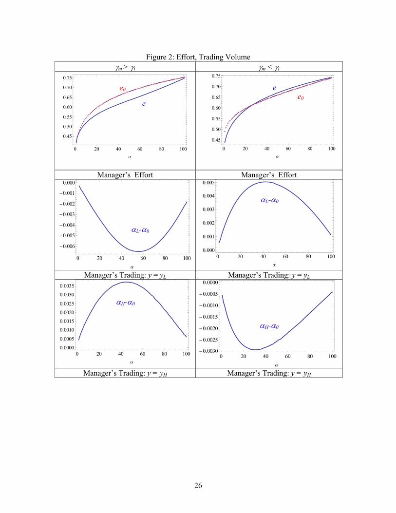
The analytical results in Section 3 show that the relative risk-aversion between the manager and the representative investor has a large impact on trading. To draw a comparison, we study two different cases for the investor’s risk tolerance: 1) γm > γi = 0.2; and 2) γm < γi = 2. In all the figures, the left-hand-side corresponds to the case with γm > γi and the right-hand-side corresponds to the case with γm < γi. For comparison, we also plot the case in which the manager is not allowed to trade with dotted curves in Figures 2, 3, and 4. Appendix D includes the analysis of this no-trade case.
Figure 1 illustrates the manager’s expected lifetime utility, U, the representative investor’s expected lifetime utility, V, and the investor’s marginal value of the stock, M, at different values of the manager’s initial shareholding. The figure shows that for both cases, γm > γi and γm < γi , the manager’s expected lifetime utility is increasing in his shareholding, while the investor’s expected lifetime utility is concave in the manager’s shareholding—it first increases then decreases in the manager’s shareholding. The case of γm > γi shows that the investor’s utility peaks at α ≈ 6%. In the case of γm < γi the investor’s utility reaches its peak at α ≈ 3%.7 The existence of the utility peaks means that investors have an optimally desired managerial ownership at t = 0. However, because the manager can trade shares, managerial ownership can quickly deviate from the optimal point. The manager’s trading strategy is illustrated in Figure 2, discussed later. Figure 1 also shows that the investor’s marginal value of the stock, M, is increasing with the manager’s shareholding in both cases; however, it increases much faster when γm < γi . This is mainly caused by the curvature of the investor’s utility function: as the investor’s shareholding decreases along the horizontal axis, his marginal utility increases faster if he is more risk-averse.
We present the manager’s strategy in Figure 2, which shows the manager’s trading volume and effort choice. Let us first examine the case with γm > γi, that is, the manager is
7 Because of the scale of the figure, the peak of the investor’s utility curve is not obvious in the case of γm < γi.
20
more risk averse. We can see that the manager buys the stock when the output is high and sells the stock when the output is low. This is consistent with the analytical results of the one-period model. The manager’s effort is increasing in his shareholdings; however, in general he makes less effort compared with his effort choice in the case where he is not allowed to trade, illustrated by the dotted e0 curve in the figure. In this case, there is a tension between risk sharing and incentive provision, and managerial trading can undermine the effectiveness of stock compensation as an incentive device. The plots on the right-hand-side present the case with γm < γi. Since the investor is more risk averse, the manager provides insurance to the investor. When output is low, the manager buys shares from the investor. As a result, the manager’s contemporaneous consumption u(cmt) decreases while his expected future utility δU(α') increases. On the contrary, when the output is high, the manager sells shares to the investor, resulting in greater contemporaneous consumption u(cmt) and lower expected future utility δU(α'). The trading results in this case are again in accord with the theoretically results in Section 3 for the one-period model. The manager chooses an effort level to maximize the sum of his contemporaneous and future utilities. Compared with the manager’s effort choice in the case where trading is not allowed (the dotted e0 curve in the figure), we find that the manager makes more of an effort when his shareholding is low and less of an effort when his shareholding is high. This finding is interesting because it is contrary to the conventional wisdom that managerial trading unravels the manager’s incentive to work hard and mitigates the power of the compensation structure.
Our trading results are different from those of DeMarzo and Urosevic (2006) who show that managerial ownership monotonically converges toward the competitive equilibrium level. Convergence in their model results from assumptions on utility functions and trading restrictions. We study a more general model that does not impose these restrictions. As a result, managerial ownership fluctuates along with output, and there is no steady state where trading stops.
Figures 3 and 4 illustrate the dynamics of the stock price, stock return, and equity premium for the two different cases, respectively. When the manager is not allowed to trade and is more risk-averse than the investor (γm > γi), the dotted curves show that the stock price and stock return are increasing, while the equity premium is decreasing in managerial shareholding. And everything is exactly the opposite when the manager is less risk-averse than the investor (γm < γi). Appendix D contains theoretical proofs of these monotonicity results. When the manager is allowed to trade, things change significantly. In the case of a more risk-averse manager (γm > γi), he sells shares when the output is low and make a smaller effort next period since effort is increasing in shareholding. As a result, the stock price conditional on the low output goes down and the stock return conditional on the low output goes up. On the other hand, the conditional stock return is lower when the output is higher. Overall, the stock is more volatile and ends up with a higher risk premium. When the investor is more risk averse (γm < γi), the opposite happens: the stock return is higher conditional on the high output and lower conditional on the low output. Consequently the stock is less volatile and the equity premium is much lower. These results conform to the analytical results summarized in Proposition 3 for the one-period case in Section 3.
21
5. Discussion
The manager’s trading behavior affects his equilibrium effort choice. This incentive effect is anticipated by the investors and reflected in their trading decisions. In this sense, the investors use the stock price as a renegotiation device to provide the manager with effort incentives. In this section, we first show that dispersed small investors cannot efficiently monitor the manger. To draw a comparison, we also study the case where small investors are replaced with one single block shareholder, who can renegotiate and monitor the manager more effectively.
5.1 Trading Behavior and Corporate Governance
Competitive trading among the continuum of small outside investors imposes a limit on the effectiveness of incentive provision. An efficient equity price, which would generate a greater incentive for managerial effort, cannot survive in a competitive environment. We now formally show this inefficiency.
Proposition 8 (Inefficiency of Market Discipline) In an SMPPE, for any trading outcome α′(α, y) ∈(0, 1), we have
.)'()(
)()'()'(
'' αα αααα
ppp
cucv
UM
mc
ic
−+= (28)
Proof: See Appendix A.
Recall that M(α) represents the marginal value of shares for the individual investor, or the derivative of the function )|ˆ(ˆ
iiV αα at ααα −== 1ˆ ii , where )|ˆ(ˆiiV αα is the lifetime
utility for an investor holding an arbitrary fraction of equity iα , while all other investors hold iα . In general, M(α) is not the same as –Vα(α), which measures the change in the representative investor’s value function in an SMPPE caused by a change in the manager’s shareholding.8 In the standard long-term contracting problem, such as the one analyzed by Spear and Srivastava (1987), an optimal contract requires that the principal and the agent have the same marginal rate of substitution between present and future payoffs, that is, Vα’(α′)/Uα’(α′) = –vc/uc. In our case, we have a continuum of investors, and the corresponding expression is –M(α′)/Uα’(α′). It would be equal to –vc/uc if (α′ – α) pα′ = 0. However, the fact that the manager trades (α′ – α ≠ 0), and more importantly, trades as a monopolist (pα′ ≠ 0) drives a wedge between the manager’s marginal rate of substitution between the current and future payoffs, uc/Uα’(α′), and that of the investors’ vc/M(α′). This implies that the necessary condition for an optimal long-term contract cannot be replicated through trading in the stock market.
8 See the discussion following equation (24) for the interpretation of M(α). The difference between M(α) and Vα(α) concerns whether only one individual investor’s shareholding changes or every investor’s shareholding changes simultaneously. M(α) is compared with –Vα(α) because αi = 1– α and dV(α)/dαi = –Vα(α).
22
Compared with a long-term optimal contract, market-based corporate control is imperfect in an SMPPE. This imperfection is due to a lack of coordination among investors, who are price takers, and thus cannot effectively set the price to induce the optimal managerial effort. The manager’s market power restricts the effectiveness of using the stock price as a renegotiation and monitoring device. The manager will take advantage of his market power and make effort choices that are not preferred by the investors. If the investors could coordinate and act as a single shareholder, then it would be possible to set the stock price to the efficient level to induce the desired managerial effort.
5.2 Block Shareholder
Now we analyze the case with a single outside investor, a blockholder. In this case, the blockholder bargains with the manager about the trading price and volume to generate the incentive for the preferred managerial effort. We consider the case in which the blockholder retains all the bargaining power and makes a take-it-or-leave-it offer to the manager. The time line of each period is as follows:
1. The manager chooses an effort level; 2. After the output is realized, the blockholder makes a take-it-or-leave-it offer to the
manager, ( tαΔ , pt); 3. The manager chooses to accept or reject the offer; 4. Consumption occurs and then the next period starts.
In the case of a single blockholder, we can also define a Strong Markov Perfect Public Equilibrium, and it is easy to check that an SMPPE consists of a set of functions, U(α), V(α), e(α), p(α, y), α′(α, y), such that, with U(α) and V(α) being the value functions for the manager and the investor, respectively, e(α), p(α, y) and α′(α, y) solve the following optimization problem:
s.t. [ ] 0)~|()~()~()~( =++− ∫ eyfUcueg eY me αδ (30)
0)]()([)]'~()~([ ≥+−+ αδααδ UyuUcu m , for any ,1'~0 ≤≤ α (31)
Constraint (30) is the first order condition for the manager’s optimal effort choice in the case where the offer is accepted. The constraint in (31) implies that the manager will accept any offer that makes him better off given that he will use the same strategy in the continuation game. It is trivial to infer that the constraint in (31) is always binding; otherwise the blockhokder could always do better by keeping α′(y) unchanged and manipulating p to reduce cm and increase ci. In other words, the blockholder will always make an offer such that the manager is indifferent between accepting and rejecting the offer. As a result, the manager will expend the same effort as in the case with no trading, and his expected lifetime utility will be the same as well. The next proposition shows that such an SMPPE exists.
23
Proposition 9 (SMPPE with a Single Blockholder) There exists a Strong Markov Perfect Public Equilibrium in which (i) the manager will exert the same effort and obtain the same utility as in the benchmark case where managerial trading is not allowed; and (ii) .
)()(
)'()'(
'
'
mc
ic
cucv
UV
−=αα
α
α
Proof: See Appendix A.
The result in Proposition 9 sharply contrasts with the case of dispersed investors. When the blockholder has the power to set trade terms, the manager and the investor can have the same marginal rate of substitution between present and future payoffs. This condition is necessary for an optimal long term contact, as in Spear and Srivastava (1987). In an SMPPE equilibrium, given the manager’s shareholding, α, the manager is always indifferent between trading or not trading. As a result, the manager will exert the same effort as in the benchmark case with no trading, and his expected lifetime utility will be the same as well. Once the output, y, is realized, the blockholder is going to trade with the manager at the consideration of two things: risk sharing and the manager’s effort incentive. Trading is essentially a renegotiation process, and the blockholder’s bargaining power makes it possible that the tension between risk sharing and incentive provision can be balanced. As a result, the manager does not extract any surplus from trading and is induced to make the effort that is desired by the blockholder.
6. Conclusion
Ownership and control are not completely separated in the real world. Certain groups of agents, managers in some firms or large shareholders in other firms, control corporate decisions and also trade in the asset market. Then there is a tension between incentive provision and risk sharing. This tension endogenously determines the pricing kernel and cash flows. In this paper, we analyze an infinite-horizon model to capture the interaction of corporate finance and asset pricing. The Strong Markov Perfect Public Equilibrium we propose enables us to use the managerial ownership as the sole state variable to characterize the dynamic processes of effort, output, and asset price. We find that managerial trading can be a source of business cycle fluctuations. When the manager is more risk-averse than the investors, output and the stock price become more volatile and the risk premium is higher; when the manager is less risk-averse than the investors, managerial trading smoothes output and results in a less volatile stock price and a lower risk premium. Our model shows that the stock price, in addition to its function as a risk allocation device, also acts as an incentive device. In absence of a long-term contract, dispersed investors renegotiate with the manager through trading in the asset market to induce managerial effort. However, a market consisting of small investors in general cannot effectively discipline the manager.
Lakonishok and Lee (2001) study the insider trading activity of all firms traded on the NYSE, AMEX, and Nasdaq during the period 1975-1995. They find that “insiders are active and that there is at least some insider trading in more than 50% of the stocks in a given year” (p. 82). Recent research by Cohen, Malloy and Pomorski (2011) argues that
24
some insider trading is not informative (that is, it is anticipated) because it is “routine,” but there is also trading that is informative. Our model predicts that insider trading conveys “inside information” to outside investors because it reveals the manager’s intended effort choice. In this sense, we focus on endogenous inside information instead of exogenous inside information.
The goal of this paper is to provide a formal dynamic framework for the analysis of agency-based asset pricing. For ease of tractability, there is only one manager and one asset in our model. If there are multiple managers and multiple assets, diversification by either managers or investors will reduce the need of risk-sharing and have an impact on managerial trading decisions and effort choices. Since idiosyncratic output shocks can change managerial holdings in different firms, these shocks will be priced. Recent empirical studies find evidence that idiosyncratic risk is indeed priced (for example, see Goyal and Santa-Clara (2003), Spiegel and Wang (2005), and Fu (2009)). Kocherlakota (1998) discusses the portfolio choice of an agent with moral hazard problem and its impact on asset prices when the agent can trade multiple stocks. An extension of our model along the same line is straightforward, but the analysis is complicated because it involves multiple state variables. Other extensions include introducing endowment shock and serial output correlation into the model. We leave these interesting questions as topics for future research.
Abowd, John and David Kaplan (1999), “Executive Compensation: Six Questions That Need Answering,” Journal of Economic Perspectives, 13 (4), 145-168.
Abreu, Dilip, David Pearce, and Ennio Stacchetti (1986), “Optimal Cartel Equilibria with Imperfect Monitoring,” Journal of Economic Theory, 39 (1), 251-269.
Abreu, Dilip, David Pearce, and Ennio Stacchetti (1990), “Toward a Theory of Discounted Repeated Games with Imperfect Monitoring,” Econometrica, 58 (5), 1041-1063.
Admati, Anat, Paul Pfleiderer, and Josef Zechner (1994), “Large Shareholder Activism, Risk Sharing, and Financial Market Equilibrium,” The Journal of Political Economy, 102 (6), 1097-1130.
Albuquerque, Rui and Neng Wang (2008), “Agency Conflicts, Investment, and Asset Pricing,” Journal of Finance, 63 (1), 1-40.
Aliprantis, Charalambos and Kim Border (1999), Infinite Dimensional Analysis, Springer.
Atkeson, Andrew (1991), “International Lending with Moral Hazard and Risk of Repudiation,” Econometrica, 59 (4), 1069-1089.
Bebchuk, Lucian and Jesse Fried (2004), Pay Without Performance: The Unfulfilled Promise of Executive Compensation, Harvard University Press
Chari, V. V. and Patrick J. Kehoe (1990), “Sustainable Plans,” Journal of Political Economy, 98 (4), 783-802.
Cohen, Lauren, Christopher Malloy, and Lukasz Pomorski (2011), “Decoding Inside Information,” Harvard Business School, Working Paper.
Core, John, Wayne Guay, and Randall Thomas (2005), “Is U.S. CEO Compensation Inefficient Pay Without Performance?” Michigan Law Review, 103 (6), 1142-1185.
DeMarzo, Peter and Branko Urosevic (2006), “Optimal Trading and Asset Pricing with a Large Shareholder,” Journal of Political Economy, 114 (4), 774-815.
Dow, James, Gary Gorton, and Arvind Krishnamurthy (2005), “Equilibrium Asset Prices Under Imperfect Corporate Control,” American Economic Review, 95 (2), 659-681.
Fu, Fangjian (2009), “Idiosyncratic Risk and the Cross-Section of Expected Stock Returns,” Journal of Financial Economics, 91(1), 24-37.
Fudenberg, Drew, David Levine, and Eric Maskin (1994), “The Folk Theorem with Imperfect Public Information,” Econometrica, 62 (5), 997-1039.
30
Fudenberg, Drew and Jean Tirole (1991), Game Theory, MIT Press.
Garen, John (1994), “Executive Compensation and Principal-Agent Theory,” Journal of Political Economy, 102 (6), 1175-1199.
Goyal, Amit and Pedro Santa-Clara (2003), “Idiosyncratic Risk Matters!” Journal of Finance, 58 (3), 975-1007.
Haubrich, Joseph G. (1994), “Risk Aversion, Performance Pay, and the Principal-Agent Problem,” Journal of Political Economy, 102 (2), 258-276.
He, Zhiguo and Arvind Krishnamurthy (2008), “Intermediary Asset Pricing,” Northwestern University, working paper.
Holmström, Bengt (2005), “Pay Without Performance and the Managerial Power Hypothesis: A Comment,” Journal of Corporation Law, 30 (4), 703-715.
Holmström, Bengt, and Paul Milgrom (1987), “Aggregation and Linearity in the Provision of Intertemporal Incentives,” Econometrica 55 (2), 303-328.
Holmström, Bengt and Jean Tirole (2001), “LAPM: A Liquidity-Based Asset Pricing Model,” Journal of Finance, 56 (5), 1837-1867.
Jensen, Michael and Kevin Murphy (1990), “Performance Pay and Top-Management Incentives,” Journal of Political Economy, 98 (2), 225-264.
Kihlstrom, Richard and Steven Matthews (1990), “Managerial Incentives in an Entrepreneurial Stock Market Model,” Journal of Financial Intermediation, 1 (1), 57-79.
Kocherlakota, Narayana (1998), “The Effects of Moral Hazard on Asset Prices when Financial Markets are Complete,” Journal of Monetary Economics, 41 (1), 39-56.
Lakonishok, Josef and Inmoo Lee (2001), “Are Insider Trades Informative?” Review of Financial Studies, 14 (1), 79-111
Lucas, Robert E., Jr. (1978), “Asset Prices in an Exchange Economy,” Econometrica, 46 (6), 1429-1445.
Magill, Michael and Martine Quinzii (2006), “Capital Market Equilibrium with Moral Hazard,” Journal of Mathematical Economics 38 (2), 149-190.
Murphy, Kevin (1999), “Executive Compensation,” chapter in Handbook of Labor Economics, Orley Ashenfelter and David Card (eds.), North-Holland, Elsevier.
Murphy, Kevin J. (2002), “Explaining Executive Compensation: Managerial Power versus the Perceived Cost of Stock Options,” University of Chicago Law Review (Summer) 69, 847-869.
Ou-Yang, Hui (2005), “An Equilibrium Model of Asset Pricing and Moral Hazard,” Review of Financial Studies, 18 (4), 1219-1251.
31
Phelan, Christopher and Ennio Stacchetti (2001), “Sequential Equilibria in a Ramsey Tax Model,” Econometrica 69 (6), 1491-1518.
Spear, Stephen E.and Sanjay Srivastava (1987), “On Repeated Moral Hazard with Discounting,” Review of Economic Studies, 54 (4), 599-617.
Spiegel, Matthew and Xiaotong Wang (2005), “Cross-Sectional Variation in Stock Returns: Liquidity and Idiosyncratic Risk,” Yale ICF working paper No. 05-13.
Stokey, Nancy L., Robert E. Lucas Jr., with Edward C. Prescott (1989), Recursive Methods in Economic Dynamics, Harvard University Press.
Sung, Jaeyoung and Xuhu Wan (2009), “Equilibrium Equity Premium, Interest Rate and the Cost of Capital in a Single-Firm Economy under Moral Hazard,” Ajou University, Working Paper.
32
Appendix A: Proofs
Proof of Proposition 1: We will only prove the case with γm > γi , as the case with γm < γi can be proved similarly. For the first part, we show that (i) if γm > γi, then the manager buys (sells) shares when y0 = y ( y ); (ii) given α0 and e, there is a unique no-trade point y* ),( yy∈ .
Differentiating (6) with respect to α1, we have:
.)|()()|()()()(
11
**1111
*11
210
*
0
* ∫∫ +−−= dyeeyfcvydyeyfcvypcvpcv
p eiciccmiccic
αα δδ .
Without the agency problem, the last term *αe is zero, and we can easily show that 0* >αp
results from the concavity of v(.). By manipulating (7), at y0 = y , we have:
.)|()1(
))(()1())((
)|()()(
)()(
)(
1*
11
*1
0*1
*1
1*1
0*1
*1
1
1*
10
11
0
11**0
*1
∫
∫
⎥⎥
⎦
⎤
⎢⎢
⎣
⎡
⎟⎟⎠
⎞⎜⎜⎝
⎛
−
+−+−−
⎟⎟⎠
⎞⎜⎜⎝
⎛ +−−=
⎥⎦
⎤⎢⎣
⎡−=−=−
dyeyfy
pyy
y
pyyy
dyeyfcvcvy
cucuy
ppp
im
ic
ic
mc
mcm
γγ
α
α
ααα
α
αααδ
δαα
Assuming *1α ≥ α0, we have 0)( *
0*1 ≥−= ααα pLHS , and for the right-hand side, we
have:
,0
)1(
))(()1())((
1*1
0*1
*1
111*1
0*1
*1
<⇒
⎟⎟⎠
⎞⎜⎜⎝
⎛
−
+−+−≤⎟
⎟⎠
⎞⎜⎜⎝
⎛<⎟
⎟⎠
⎞⎜⎜⎝
⎛≤
⎟⎟⎠
⎞⎜⎜⎝
⎛ +−−
RHS
y
pyy
y
y
y
y
y
pyy iimm γγγγ
α
ααα
α
ααα
which is a contradiction. Therefore, we must have *1α < α0 with γm > γi and y0 = y .
Similarly, we must have *1α > α0 with γm > γi and y0 = y .
The existence of a no-trade point, y*, is the result of the Mean Value Theorem. For uniqueness, at y* we have:
0)|( 1*
11
*
1
*
1 =⎥⎥⎦
⎤
⎢⎢⎣
⎡⎟⎟⎠
⎞⎜⎜⎝
⎛−⎟⎟
⎠
⎞⎜⎜⎝
⎛= ∫ dyeyf
yy
yyyRHS
im γγ
.
Rearranging the above equation, we get:
∫∫
−
−
− =1
*1
11
1*
11
1*
)|(
)|()(
dyeyfy
dyeyfyy
m
i
im
γ
γ
γγ .
33
Since imy γγ −)( * is monotonic in y*, there is a unique no-trade point y* at which *1α = α0.
Further, continuity implies that *1α > α0 when y > y* and *
1α < α0 when y < y*.
For the second part, if the manager is a price-taker, then (7) becomes:
.0)|()()( 1*
1110 =+− ∫ dyeyfcuycpu mcmc δ
At the same time, (6) can be rewritten as:
.0)|()()( 1*
1110 =+− ∫ dyeyfcvycpv icic δ
Let us denote the equilibrium managerial shareholding as **1α in this case. Then we have,
at y0:
.)|()1(
))(()1())((0 1
*1
1**
1
00**
10**
1
1**
1
00**
10**
11∫ ⎥
⎥⎦
⎤
⎢⎢⎣
⎡⎟⎟⎠
⎞⎜⎜⎝
⎛
−+−+−
−⎟⎟⎠
⎞⎜⎜⎝
⎛ +−−= dyeyf
ypyy
ypyy
yim γγ
αααα
αααα
δ
Since the right-hand-side is exactly the same as in the case where the manager is a monopolistic trader, the no-trade point still holds. We can further prove that the RHS is a decreasing function of **
1α :
.0)1(
1)1(
))(()1()(
))((
)1())(()1())((
1
02**
1
0
1
1**
1
00**
10**
1
1
02**
1
0
1
1**
1
00**
10**
1
1**
1
00**
10**
1
1**
1
00**
10**
1**
1
<+
−−
⎟⎟⎠
⎞⎜⎜⎝
⎛−
+−+−−
+⎟⎟⎠
⎞⎜⎜⎝
⎛ +−−−=
⎥⎥⎦
⎤
⎢⎢⎣
⎡⎟⎟⎠
⎞⎜⎜⎝
⎛−
+−+−−⎟⎟
⎠
⎞⎜⎜⎝
⎛ +−−∂
∂
−−
ypy
ypyy
ypy
ypyy
ypyy
ypyy
im
im
im αα
ααααγ
αα
ααααγ
αααα
αααα
αγγ
γγ
When y0 > y*, we have *1α > 0α and RHS > 0 when the manager is a monopolistic trader,
so we must have **1α > *
1α to drive RHS down to zero in the case where he is a price taker. Similarly, when y0 < y*, we have *
1α < 0α and RHS < 0, so we must have **1α < *
1α to drive RHS up to zero.
Proof of Lemma 1: The optimal effort choice, e, satisfies the first order condition:
∫ =+−Y ee dyeyfyueg .0)|()()( α
We assume that the second order condition holds:
∫ <+−Y eeee dyeyfyueg .0)|()()( α
Taking the derivative of the first order condition with respect to α gives:
∫ ∫ =++−Y Y eceeee dyeyfyyudyeyfyuege .0)|()(])|()()([ ααα
This implies that eα > 0 if and only if ∫ >Y ec dyeyfyyu 0)|()(α .
34
Plugging in ,1
)(1
m
mm
mccu
γ
γ
−=
−
∫ ∫−
=Y Y e
mec dyeyfyudyeyfyyu )|()(
1)|()( α
αγ
α . Since
MLRC guarantees that ∫ =Y ee egdyeyfyu )()|()(α > 0, we have eα > 0 if and only if γm <
1. For a general utility function, Appendix D shows that the condition for eα > 0 is that yuc(αy) is increasing in y.
Proof of Proposition 2: For (i), let us prove the existence of a no-trade point by construction. Let y* be the no-trade point for the case without the agency problem, and in particular, with the effort choice equal to )( 0
* αe , the optimal effort choice when 0*1 αα =
in the case with the agency problem. It is easy to check that the triplet ( ))( ),(, 0
*0
*0
*1 αααα ep= satisfies the equilibrium conditions in (4), (5) and (6). Therefore,
there exists a no-trade point y*** ),( yy∈ coinciding with the corresponding no-trade point
without the agency problem, y*( ))(, 0*
0 αα e . The proof of uniqueness is the same as Proposition 1, and is thus omitted.
Next we prove part (ii). Differentiating (6) with respect to α1, we have:
.)|()()|()()()(
11
**1111
*11
210
*
0
* ∫∫ +−−= dyeeyfcvydyeyfcvypcvpcv
p eiciccmiccic
αα δδ .
In the above equation, the effect of the agency problem is captured by the last
term ∫ 1**
111 )|()( dyeeyfcvy eic α . Similar to the proof of Lemma 1 (also see the proof of
Lemma D1 in Appendix D), we can show:
.1 ifonly and if 0)|()( 1**
111 <>∫ ieic dyeeyfcvy γα
Therefore, in the case of γi <1 the value of *αp is positive and greater than in the case
without the agency problem. Similar to the Proof of Proposition 1, we can show that the manager buys (sells) shares when y0 >(<) y* if γm > γi,, and sells (buys) shares when y0 >(<) y* if γm < γi.
In the case of γi > 1 > γm, the value of *αp is smaller, and we proceed to prove that part (ii)
holds as long as αeeyfeyfe
)|()|(
is bounded.
The last two terms of *αp can be combined as:
.)|(
)|()(
)|()()|()(
1*1
**1
111
1**
1111*
1121
∫
∫∫
⎥⎦
⎤⎢⎣
⎡+=
+−
dyeyf
eeyfcvy
dyeeyfcvydyeyfcvy
e
i
iic
eicicc
α
α
αγ
δ
δδ
35
When α0 is close to 1, αi1 is close to zero (the investor cannot buy many shares due to the wealth constraint and cannot sell many shares due to the short sale constraint),
)|()|(*
1
**1
1 eyfeeyfe
i
i α
αγ
+ is positive and accordingly *αp is positive. Similar to what we have
shown in the proof of Proposition 1, we must have the manager selling shares when y0 = y and buying shares when y0 = y if α0 is close to 1. Because y0 = y or y cannot be a no-trade point, the manager sells shares when y0 = y and buys shares when y0 = y for all other values of α0. Combining this with the uniqueness of the no-trade point, we know that the manager sells (buys) shares when y0 >(<) y* .
Now let us prove part (iii). Let ***1α be the manager’s optimal choice of α1. By
manipulating (7), at y0, we have:
.)|()1(
))(()1())(()( 1
*1
1***
1
00***
10***
1
1***
1
00***
10***
11
*0
***1 ∫ ⎥
⎥⎦
⎤
⎢⎢⎣
⎡⎟⎟⎠
⎞⎜⎜⎝
⎛
−+−+−
−⎟⎟⎠
⎞⎜⎜⎝
⎛ +−−=− dyeyf
ypyy
ypyy
ypim γγ
α αααα
αααα
δαα
We only examine the case where 1> γm > γi and y0 < y*. All other cases can be proved similarly. From the proof of part (ii), we know when γm > γi and y0 < y*, the manager sells shares, that is, ***
1α < α0. In addition the value of *αp is greater than that in the case
without the agency problem. If the manager trades more aggressively than in the case without the agency problem, that is, ***
1α ≤ *1α , we will have that LHS is smaller while
RHS is greater than in the case without the agency problem (from the proof of Proposition 1, we know that RHS of the above equation is a decreasing function of ***
1α ). The equation above cannot hold; a contradiction. Therefore, we must have ***
1α > *1α ,
that is, the manager will sell less aggressively.
Proof of Proposition 3: For (i), with γm < γi, the manager is less risk averse than the investor, and he provides insurance to the investor. When the date 0 output is higher (lower) than the no-trade point, the manager sells (buys) shares, the next period’s effort choice is lower (higher), and it is less likely to have a high (low) output; and this automatically generates a mean reverting pattern in outputs. For (ii), with γm > γi, the manager is more risk averse than the investor, and he smoothes consumption with the investor providing liquidity. When the date 0 output is higher (lower) than the no-trade point, the manager buys (sells) shares. Accordingly, the next period’s effort choice is higher (lower), and it is more likely to have a high (low) output. So managerial trading amplifies the economic fluctuations.
Proof of Proposition 4: We know that:
.0]|),()([)(
1 *111
0
=Π eycvEcv ic
ic
αδ
With CRRA preferences for the investor, differentiating the above equation with respect
36
to α1 gives:
,0]|),()([ *111 =eygcvE ic α
where )|()|(),(),(),(
1
1111111 eyf
eyfeyyyg eαα ααα Π+Π= .
It is easy to check that πα(α1) = E[g(α1, y1)|e*]. We know:
].|),([]|)([
]|),([]|)([]|),()([
]|),(),([
*11
*1
*11
*1
*111
*111
eygEecvE
eygEecvEeygcvE
eygcvCOV
ic
icic
ic
α
αα
α
−=
−=
Since vc(ci1) is always positive, we have E[vc(ci1)|e*] > 0. This means COV[vc(ci1), g(α1, y1)|e*] and E[g(α1, y1)|e*] have different signs. Since vc(ci1) is decreasing with y1, when g(α1, y1) is increasing (decreasing) with y1, we have COV[vc(ci1), g(α1, y1)|e*] < 0 (>0) and E[g(α1, y1)|e*] > 0 (< 0). Without the agency problem, ),(),( 1111 yyg αα αΠ= and is decreasing
with y1 because .0))((
/),(/),( 21
*
*
111111 <−=∂Π∂=∂Π∂α
ααα αα p
pyyy y With the agency
problem, g(α1, y1) may increase with y1 because eα>0, Π(α1, y1) is increasing in y1, and MLRC implies fe(y1|e)/f(y1|e) is increasing in y1.
Proof of Proposition 5: We first prove that Mt+1 is bounded above. The representative investor's decision problem is:
])([max0
1∑
∞
=∞=
tit
t cvEtt
δα
s.t. .)( 1 titittitit pyc ααα −−= +
Taking the derivative with respect to αit+1, for t ≥ 0, we have:
,1
)]])([
)]]()([)([)]()([)(
11
222111
111
cts
cts
tsiscs
tst
itctttitctt
itcttttitc
vyvycvyE
cvpyEcvyEcvpyEpcv
δδδδ
δδδδ
−=≤=
++=+=
∑∑∞
+=
−∞
+=
−
++++++
+++
which implies that )(1 yv
vypc
ct δ
δ−
≤ for any t ≥ 0. Consequently, we have:
.)()1(
)]()[( 1111
∞<⎟⎟⎠
⎞⎜⎜⎝
⎛−
+≤
+= ++++
cc
c
itctttt
vyv
vyy
cvpyEM
δδ
Next, we prove the equivalence between the outcome of the auxiliary dynamic competitive equilibrium and that of the static one-period equilibrium. The necessity part
37
is trivial. We now prove sufficiency. Assume ),(),( *1
***+∈ tititit MCEc αα . Then, a necessary
condition for ),( **ititc α to be the equilibrium outcome is:
( ) ].1,0[ allfor ,0)()( 1*
11*
1** ∈≤−+− ++++ ititittitct αMcvp ααδ
This implies that:
)].([
)])(([*
11*
11
*11
**1
+++−
++−
−−≤
−−
itittt
itititctt
ME
cvpE
ααδ
αα
Add )]([)])(()[( **1
***1 ititttitittcttt MEcvpyE αααα −=−+ −− to each side of the above
Since *tM is bounded from above, we have [ ] 0)]()([lim
0* ≤−∑ =∞→
T
t ititt
T cvcvE δ , and
),( **ititc α is optimal.
Proof of Proposition 6: Given the pricing function p(α, α’, y) and the value function U(α), the manager of the firm chooses effort choice, e, and next period’s shareholding, α’, to maximize his utility. Let CU be the set of continuous functions from [0, 1] to R, and let ρ be the sup-norm defined on CU, that is ρ(U1, U2)=sup ]1,0[∈α U1(α) – U2(α). Given continuous p(α,α’,y) and U(α), define a mapping TU: CU→CU as follows:
.),',()'(..
)|(])'()([max)(max))(( '
ypycts
dyeyfUcuegUT
m
Y meU
ααααα
αδα α
−−=
++−= ∫
We can show that TU(U) is a contraction mapping. According to Berge’s Maximum Theorem, we know that the fixed point U is a continuous function, and, moreover, the corresponding solution E(α) for the effort choice and A’(α, y) for the trading strategy are
38
compact-valued upper hemi-continuous correspondences (E(α) and A’(α, y) are not empty-valued as the objective function is continuous and the choice sets are compact by the Extreme Value Theorem). We know that a compact-valued upper hemi-continuous correspondence contains a continuous function, 9 and we can pick such continuous functions from E(α) and A’(α, y), defined as e(α) and α’(α, y), respectively. Therefore, we have a map from a continuous pricing function p(α, α’, y) to e(α), α’(α, y), which is also continuous.
Given continuous e(.), α’(.), define:
).','','()'''(')'1(')'('
)','('''..
')'|'()]','','(')['([)')((
ypycee
yts
dyeyfypycvpT
i
Y icp
αααααα
ααα
ααδα
−+−==
=
+= ∫
Let Cp be the set of continuous function from [0,1]2× ],[ yy to R, and let ρ be the sup-norm define on Cp, we can show Tp(.) is a contraction mapping, and there exists a continuous function p(α,α’,y) such that, vc(ci)p=Tp(p) with ci = (1– α)y + (α’ – α) p(α, α’, y). Thus, we establish a mapping from e(α), α’(α,y) to p(α, α’, y).
With Cp being the set of continuous pricing functions defined on [0,1]2× ],[ yy , so far we have established a mapping from p(α, α’, y)∈Cp to p(α, α’, y) ∈ Cp, which we call T. We can show that Cp is a non-empty weakly compact convex subset of a Banach space (because the set of continuous functions defined on a compact set with the sup-norm is compact, convex, and complete), and T is a continuous mapping as it is the product of two continuous mappings. By the Brouwer-Schauder-Tychonoff Fixed Point Theorem,
we know there exists a fixed point p(α, α’, y)∈Cp([0,1]2× ],[ yy ) such that p∈T(p). 10
Proof of Proposition 7: To prove the existence of no-trade point, we first show the following lemma.
Lemma A1: For two continuous function x1(y) > 0 and x2(y), if ∫=Y
dyyxX )(11 and
∫=Y
dyyxX )(22 , then there exists y*∈Y such that X2/X1 = x2(y*)/x1(y*).
Proof: Assume x2(y)/x1(y) > X2/X1 for all y ∈ Y, then we have ∫=Y
dyyxX )(22 >
∫ =Y
XdyXXyx 2
1
21 )( , a contradiction. Similarly, it is not possible x2(y)/x1(y) < X2/X1 for all
9 To see this, we know that a compact-valued upper hemi-continuous correspondence (Ω: X→Y) has the following property: for every sequence xn→x and every sequence yn such that yn∈Ω(xn) for all n, there exists a convergent subsequence of yn whose limit point y is in Ω(x). See, for example, Stokey and Lucas (1989). 10 See, for example, Aliprantis and Border (1999).
39
y∈Y. By the Mean Value Theorem, we know that there exists some y* such that X2/X1 = x2(y*)/x1(y*).
With Lemma A1, we can prove the existence of a no-trade point as follows. Taking the derivative with respect to α for (22), and using the Envelope Theorem, we have:
∫ −−+=Y mc dyeyfppycuU .)|(])'()[()( αα ααα
Applying Lemma A1 to the above equation for Uα(α) and equation (24) for M(α) , we know that there exists a y*(α)∈Y, such that:
.))((
])'()[()()(
***
*****
pycvppycu
MU
ic
mc
+−−+
= αα αααα
On the other hand, the first order condition for (26) implies:
,])'()[(1)'( 10*
'' λλααδ
α αα +−−+= ppcuU mc
where λ0(α, y) ≥ 0 and λ1(α, y) ≥ 0 are Lagrange multipliers for the constraints α′ ≥ 0 and 1 – α′ ≥ 0. And equation (27) shows that:
).~(),'~,(1)'~( ic cvypM ααδ
αδ =
At y*(α), we have α′* = α′(α, y*(α)) satisfying the following condition:
)(])'()[(
)'()'(
**
*1
*0
*'
***
*
*'
ic
mc
cvpppcu
MU λλαα
αα αα +−−+
= .
Comparing the above equation with the one for )()(
ααα
MU at y*(α), we can see that α′* = α is
a solution for α′(α, y*(α)), at which λ0(α, y) =0, λ1(α, y) =0 and )()(
)'()'(
*
*'
αα
αα αα
MU
MU
=
=)()(
ic
mc
cvcu . Therefore, y*(α) is a no-trade point.
As for the monotonicity of the manager’s effort with respect to his shareholding, we differentiate the first order condition for (25) with respect to α and have:
∫∫ =−−++⎥⎦⎤
⎢⎣⎡ +−
∂∂
Y emcY eemee dyeyfcuppydyeyfcuege .0)|()(])'([)|()()( αααα
Notice that α’∈(0, 1) guarantees ∂(u(cm) + δU(α′))/∂α′ = 0 from the first order condition for (26), and that eliminates the ∂α′/∂α term from the above expression.
We can see that ∂e/∂α > 0 iff ∫ >−−+Y emc dyeyfcuppy 0)|()(])'([ ααα , since
∫ <+−Y eeee dyeyfyueg 0)|()()( α is assumed for the optimality of e. Similar to the proofs
40
of Lemma 1 and Lemma D1, MLRC implies that uc(cm)[y + p – (α′ – α) pα] increasing in y is a sufficient condition for ∂e/∂α > 0.
Proof of Proposition 8: From equation (27), we know that:
.)(1)'( pcvM icδα =
With Lagrange multipliers λ0(α, y) ≥ 0 and λ1(α, y) ≥ 0 for the constraints α′ ≥ 0 and 1 – α′ ≥ 0 respectively, the first order condition for (26) implies:
.])'()[(1)'( 10*
' λλααδ
α αα +−−+= ppcuU mc
For α′(α, y)∈(0, 1), λ0 = λ1 = 0. The result is immediate.
Proof of Proposition 9: Since the constraint in (31) is binding, we have:
,0
)|()([)(
)|()()|()([)(
)|()]()([)(
)|()'()([)(
=
+−=
++−=
++−=
++−
∫∫∫
∫∫
Y ee
Y eY ee
Y ee
Y eme
dyeyfyueg
dyeyfUdyeyfyueg
dyeyfUyueg
dyeyfUcueg
α
αδα
αδα
αδ
where ∫Y e dyeyf )|( =0 follows 1)|( =∫Y dyeyf . The first order condition is exactly the
same as the one for the benchmark case with no trade characterized in Appendix D, so the manager makes the same effort and gets the same expected utility as in the benchmark case with no trade.
subject to constraints (30) and (31). Given U(.) = U0(.), with U0(.) being the value function with no trade, it is easy to show that T(V) satisfies Blackwell's sufficient conditions (monotonicity and discounting) for being a contraction mapping for any bounded function V(.) defined on [0, 1]: (i) Monotonicity: For all α∈[0, 1], V1(α) ≤ V2(α) implies T(V1)(α) ≤ T(V2)(α); (ii) Discounting: T(V+c)(x) ≤ T(V)(x) + δc, for any c ≥ 0.
In equilibrium, with the optimal α′ and p, we also can represent the manager’s and the investor’s value functions with the following Bellman equations:
∫ ++−=Y m dyeyfUcuegU )|()]'()([)()( αδα
41
.)|()]'()([)( ∫ +=Y i dyeyfVcvV αδα
Pointwise variations in α′ and p for the above two equations give:
.0')'(')()')((
0')'(')()')((
'
'
=++−
=+−−−
pV
ppcvcv
pU
ppcucu
icic
mcmc
ΔαΔαδ
ΔαΔαα
ΔαΔαδ
ΔαΔαα
α
α
So we have .)()(
)'()'(
'
'
mc
ic
cucv
UV
−=αα
α
α
42
Appendix B: Factorization of the Game
Given the initial shareholding of the manager α∈[0, 1], define Γ(α) to be the set of values which the manager and the representative investor can obtain and the marginal value of shares for the investor from a symmetric sequential equilibrium:
.)(economy for the PPE a is |])[]),[],[())(),(),(()( ασσσσαααα Φ==Γ MVUMVU
Characterizing the PPE requires the factorization of the Γ(α) into a stage payoff and a continuation payoff, a step that is necessary in order to write the equilibrium outcomes recursively (see Abreu, Pearce, and Stacchetti (1990)). We provide this characterization in this appendix, following Abreu, Pearce and Stacchetti (1990). We demonstrate the factorization of Γ(α) for the game with a continuum of investors below.
Let W: [0, 1]→R³ be an arbitrary value correspondence, which is compact and convex.
Definition B1 A vector ζ1 = (α′(y), U′(y), V′(y), M′(y)) is said to be consistent with respect to W at the initial shareholding α∈[0, 1] if the following conditions are satisfied:
1. Generation: (U′(y), V′(y), M′(y))∈W(α).
2. Short Sale Constraint: α′(y)∈[0, 1] for any y∈Y.
3. Investor Optimality: (αi′(y), ci(y))∈CE(1 – α, M′(y)) with price p(y), where αi′(y) = 1 – α′(y) and ci(y) = (1 – α)(y + p(y)) – (1 – α′(y))p(y).
The investor’s optimality in a competitive market requires –p(y)vc(ci(y)) + δM′(y) = 0 (first order condition), which determines p(y) once M′(y) is set. Given α′, for each y∈Y, let:
]'~)~([min)',,( )'~,'~,'~( UcuyU mMVU δαα +≡
s.t. )'~,'~,'~,'(~1 MVUαζ = is consistent with respect to W at α,
and .~')~(~ ppycm αα −+=
U(α, y, α′) gives us the worst possible payoff for the manager, and this is used to define the punishment value for the manager when he deviates from the equilibrium path.
Define ).'ˆ,,(max),( 'ˆ ααα α yUyU ≡ Therefore, ),( yU α is the best alternative value to the manager when he deviates from the equilibrium.
Definition B2 A consistent vector ζ = (e, ζ1) is said to be admissible with respect to W at the initial shareholding α if ζ1 is consistent with W at α and the following two conditions are satisfied:
]ˆ|)('))(()ˆ([max]|)('))(()([ ˆ eyUycuegEeyUycuegE mem δδ ++−≥++− ,
).,()('))(( yUyUycu m αδ ≥+
43
Admissibility adds the manager's incentive constraint to the requirements for consistency; the first inequality implies that the manager will make the optimal effort choice given his trading behavior, and the second inequality requires the manager to trade optimally. When the manager trades an unexpected fraction of equity, the investor’s beliefs are updated in the subsequent subgame so as to yield the worst possible payoff for the manager. This is without loss of generality. If an equilibrium is sustainable with another type of punishment upon deviation, then it must also be sustainable with the worst punishment upon deviation. This is the same concept as what Chari and Kehoe (1990) call a “sustainable equilibrium.”
The vector ζ = (e, α′(y), U′(y), V′(y), M′(y)) gives the following payoff values to the manager and the investor and the marginal value of the shares to the investor:
].|))(())([(),(
],|)('))(([),(
],|)(')),(([),(
eycvypyEM
eyVycvEV
eyUeycuEU
ic
i
m
+≡
+≡
+≡
ζα
δζα
δζα
(
(
(
Let )),(),,(),,((),( ζαζαζαζα MVU(((
≡Ξ , and for a value correspondence W, define:
.at respect to with admissible is |),())(( αζζαα WWB Ξ=
Lemma B1 If W has a compact graph, then B(W) has a compact graph.
Proof: First, we can show that B(W) has a bounded graph. It is easy to see that
]/)(,/)([)( δδα yvyvV ∈ and ])()(,)()(
[)(δδ
α yuegyuegU +−+−
∈ . Also we have
shown in the proof of Proposition 5 that M is bounded from below and above.
Second, we can show that B(W) has a closed graph. Let wn, αn be a sequence in the graph of B(W) which converges to a point (w, α). We need to show that (w, α) is also in the graph of B(W). By the definition of B(W), there exists a sequence of vectors ζn = en, αn′(y), Un′(y), Vn′(y), Mn′(y) admissible with respect to W at αn, and wn = Ξ(αn, ζn) satisfying the short-sale constraint, price consistency, and incentive compatibility. Because the space of admissible stage strategies and value functions are bounded, we may assume this sequence converges to some limit point ζ = e, α′(y), U′(y), V′(y), M′(y), where the convergence of functions αn′(y), Un′(y), Vn′(y), and Mn′(y) is almost everywhere.
The convergence of the sequence en is trivial to show. To show the almost-everywhere convergence of αn′(y), Un′(y), Vn′(y), and Mn′(y), we proceed as follows. First, all these functions are bounded on Y, which is itself bounded. Therefore, these functions are in Lp-space. It is easy to find a Cauchy subsequence for each of them, say gn, and we know that there exists a function g in Lp-space with a Lp-norm, s.t.
0||||lim →−∞→ pnn gg . Second, 0||||lim →−∞→ pnn gg in Lp-space implies that there exists a subsequence hn of gn, such that hn converges to g almost everywhere. This guarantees that g is a feasible function, that is, it is constrained by the same bounds as that for the original function sequence, αn′(y), Un′(y), Vn′(y), or Mn′(y).
44
By continuity of Ξ, we know that Ξ(α, ζ) = w, and ζ is admissible with respect to W at α. Therefore, (w, α) is in the graph of B(W).
Following Phelan and Stacchetti (2001), we can show that Γ(α) = B(Γ)(α) for all α, and Γ(α) is the largest value correspondence W such that W = B(W)(α). For each α, define W∞(α) = B(B(...(B(W)))(α) = B∞(W)(α), and with the compactness property of B(.), we can show W∞(α) = Γ(α).
45
Appendix C: Algorithm for the Numerical Examples
It is easy to show that in an SMPPE, we have the following Bellman equations:
∫ ++−=Y m dyeyfyUcuegU ,))(|())],('()([))(()( αααδαα
∫ +=Y i dyeyfyVcvV ,))(|())],('()([)( αααδα
.))(|()),('()),,(',(
)),,(',()( dyeyfyMyyp
yypyMY
αααδααα
αααα ∫+
=
These Bellman equations will be used for our numerical examples.
Define a grid α1, ..., αN and solve for the value functions of U0(α), V0(α) and M0(α) assuming that the manager is not allowed to trade.Starting from the solved functions U0(α), V0(α) and M0(α) as the initial functions, we map (Ut(α), Vt(α), Mt(α)) to (Ut+1(α), Vt+1(α), Mt+1(α)) as follows:
• Step 1: For each αk, k = 1, ..., N, given the output y, find the optimal α′ to maximize u(cm) + δUt(α′) with p determined by the first order condition in equation (27) using Mt(α′);
• Step 2: Find the optimal effort choice, e, of the manager given the optimal α′ and the resulting p for each y;
• Step 3: Define:
].|)'([)(
],|)'()([)(
],|)'()([)()(
1
1
1
eMp
pyEM
eVcvEV
eUcuEegU
t
ti
t
tm
t
αδα
αδα
αδα
+=
+=
++−=
+
+
+
Repeat Steps 1-3 until (U, V, M) converges, and then generate sample equilibrium paths based on the limit (U, V, M).
46
Appendix D: No Trading Case
In this appendix, we analyze a benchmark case in which the manager is not allowed to trade shares in the stock market. It is infinite horizon, and each period the manager makes an effort choice that determines the distribution of the output, f(y|e). We assume the f(y|e) satisfies the Monotone Likelihood Ratio Condition. After the output is realized, it is given out as dividends to the manager and the investors based on the number of shares they hold. The manager’s effort choice is influenced by the fraction of the equity he owns. Equity prices are decided in a competitive market with a continuum of outside investors.
For a given managerial ownership α, the manager chooses an effort level to maximize his lifetime utility:
∫
∑
++−=
+−=∞
=
Ye
ttmtt
te
Udyeyfyueg
ecuegEUt
).()|()]()~([max
]|)()([max)(
0~
00
αδα
δα
The optimal effort choice, e, satisfies the first order condition:
∫ =+−Y ee dyeyfyueg .0)|()()( α
We assume that the second order condition holds:
∫ <+−Y eeee dyeyfyueg .0)|()()( α
The next two lemmas discuss the manager’s effort choice and trading incentive, respectively.
Lemma D1 (The Manager’s Effort Decision) If the manager's utility function satisfies the condition that yuc(αy) is increasing (decreasing) in y, then the optimal effort level, e, is increasing (decreasing) in the manager’s shareholding, α.
Proof: Taking the derivative of the first order condition with respect to α gives:
∫ ∫ =++−Y Y eceeee dyeyfyyudyeyfyuege .0)|()(])|()()([ ααα
We assume ∫ <+−Y eecee dyeyfyyueg 0)|()()( α so that there is an interior solution for e.
Following this assumption, we have eα > 0 iff ∫ >Y ec dyeyfyyu 0)|()(α .
Write: ∫ ∫=Y Y
ecec dyeyf
eyfeyf
yyudyeyfyyu .)|()|()|(
)()|()( αα
47
Since ,1)|(∫ =Y
dyeyf we have .0)|()|()|()|()|(
∫∫∫ =∂∂
==YY eY
e dyeyfe
dyeyfdyeyfeyfeyf
The Monotone Likelihood Ratio Condition (MLRC) implies that there exists a y* such that fe(y|e)/f(y|e)>0 iff y > y*. If yuc(αy) is increasing in y, then we have:
.0
)|()|()|()(
)|()|()|()()|(
)|()|()(
)|()|()|()()|(
)|()|()(
)|()|()|()(
**
****
=
=
+>
+=
∫
∫∫
∫∫
∫
><
><
Ye
c
y*ye
cy*ye
c
y*ye
cy*ye
c
Ye
c
dyeyfeyfeyfyuy
dyeyfeyfeyfyuydyeyf
eyfeyfyuy
dyeyfeyfeyfyyudyeyf
eyfeyfyyu
dyeyfeyfeyfyyu
α
αα
αα
α
Similarly if yuc(αy) is decreasing in y, we have .0)|()|()|(
)( <∫Ye
c dyeyfeyfeyf
yyu α
Lemma D2 (The Manager’s Incentive to Trade) If the manager and the investors have CRRA preferences with the manager’s risk-aversion coefficient, γm, different from the investors’ risk-aversion coefficient, γi, then the manager has an incentive to trade.
Proof: The expected utility of the manager is given by ∑∞
=
+−=0
]|)()([)(t
t eyuegEU αα , where
e is the optimal effort level in the equilibrium. Without loss of generality, we assume α∈(0, 1) and we consider a one shot deviation after yy = is realized. The manager is facing the following optimization problem:
)]'([)(max ' αδα UEcu m +
s.t. ).()'( ypycm ααα −+=
The first order condition with respect to α′ is:
.0)'()()( ' =+− αδ αUypcu mc
The Envelope Theorem tells us that:
∑ ∫∞
=
=0
' .))'(|()'()'(t
Y tttctt dyeyfyuyU ααδαα
Given α, the investors' trading determines the equity price:
∑∞
=
−−
=1
)].(|))1(([))1((
1)(t
tctt
c
eyvyEyv
yp ααδα
48
It is easy to check that, with CRRA preferences, at α′ = α, the first order derivative with respect to α′ is:
[ ]
( )[ ],1
1
))1(('))1(('
)(')('1
)(')()('
1
11
mimiim
imimm
yyyE
yyyE
yvyv
yuyuyEUypcu
γγγγγγ
γγγγγ
αδ
δ
αδ
δ
αα
ααδ
δαδ
−−−−
−−−−
−−
=
−−
=
⎥⎦
⎤⎢⎣
⎡⎟⎟⎠
⎞⎜⎜⎝
⎛−
−−
−=+−
which is > 0(< 0) if γm > γi (γm < γi). Therefore, we can see that the manager in general will have an incentive to trade in the market as long as γi ≠ γm even though they are forbidden to do so.
Proposition D1 (Asset Prices) Assume the investor has a constant Arrow-Pratt measure of relative risk aversion, then: (i) if both yvc(ci) and yuc(cm) are monotonic in y and
)0(0)()(<>
∂∂
∂∂
ycyu
ycyv mcic , then the equity price is increasing (decreasing) in α ; and (ii)
if yuc(cm) is increasing (decreasing) in y, then the price of the risk free bond is decreasing (increasing) in α and the risk free interest rate is increasing (decreasing) in α.
Proof: Given α and y, the price of equity is:
∫
∫
−=
+=
Yic
ic
Yic
ic
dyeyfcvcv
y
eyfypycvcv
yp
'.)|'()()'(
'1
),|'()]',('[)()'(
),(
δδ
αδ
α
where ci and ci′ denote the investor’s consumption in the current period and the next period, respectively. We do not explicitly have a bond in the economy, but that is equivalent to assuming that a bond is in zero net supply and thus no one trades the bond in a symmetric (among investors) equilibrium. The price of a risk free zero-coupon bond is:
∫≡Y
ic
ic eyfcvcvyb ).|'(
)()'(),( δα
For (i), differentiating the equity price with respect to α gives us:
.')|'()'(')(')|'()'(')()(
1
')|'()'(')(
1),(
22 ∫ ∫
∫
+−+
=
Y Y icicciccicic
Y eicic
dyeyfcvycyvdyeyfcvycvcv
dyeyfecvycv
yp
δδ
δα αα
With a constant Arrow-Pratt measure of relative risk aversion for the investor, the last two terms sum to zero and we have: