Agency Theory and Firm Value in India

Jayesh Kumar∗

Indira Gandhi Institute of Development Research,

Gen. A. K. Vaidya Marg, Goregaon (East), Mumbai 400 065

E-mail : jayesh@igidr.ac.in

∗The author is grateful to Kausik Chaudhuri, Joseph P. H. Fan, Stijn Claessens, and the participants of theSixth International Conference of The Association of Asia-Pacific Operational Research Societies (APORS) atIIT Delhi, Regional Network Meeting of Global Corporate Governance Forum (GCGF), World Bank at ISBHyderabad, and the Seventh Capital Markets Conference at IICM Navi Mumbai for helpful suggestions andcomments. Usual disclaimer applies.

Agency Theory and Firm Value in India

ABSTRACT

This paper examines empirically the effects of ownership structure on the firm perfor-

mance for a panel of Indian corporate firms, from an ‘agency perspective’. We examine

the effect of interactions between corporate, foreign, institutional, and managerial owner-

ship on firm performance. Using panel data framework, we show that a large fraction of

cross-sectional variation, in firm performance, found in several studies, can be explained

by unobserved firm heterogeneity. We provide some evidence that the shareholding by in-

stitutional investors and managers affect firm performance non-linearly, after controlling

for observed firm characteristics and unobserved firm heterogeneity. We also find that the

equity ownership by dominant group influences firm-performance. We find no evidence

in favor of endogeneity of shareholding pattern.

JEL Classification:G32; G34.

Keywords:Corporate governance, Shareholding pattern, Firm performance, Panel Data,

India.

1

In this paper, we examine whether differences in ownership structure across firms can

explain their performance differences in an emerging economy like India. Using detailed

ownership structure of more than 2000 Indian corporate firms over the period 1994-2000,

we provide answer to some of the questions raised herewith. Does ownership matter? If it

does, then, whether government ownership is more effective than private (including foreign)

ownership in maximizing firm value? Does the identity of shareholder matter? What is the

comparative efficiency of several forms of private ownership? What is the preferred ownership

structure for privately held firms? Is ownership structure really endogenous? Can ownership

be a tool to control agency cost?

These are some of the important questions, which researchers are trying to explore in the

recent literature of corporate finance. In this context, we investigate Indian corporate firms in

order to provide new evidence on how ownership structure influence firm value.

Corporate Governance is the system of control mechanisms, through which“the supplier

of finance to corporations assure themselves of getting a return on their investment,”(Shleifer

and Vishny (1997)). The classical problem lies within the separation of ownership and con-

trol, i.e. the agency cost resulting from a divergence of interest between the owners and the

managers of the firm (Jensen and Meckling (1976)).

Researchers have extensively studied the conflict between managers and owners regard-

ing the functioning of the firm, although, the research on understanding the differences in

behavior of different shareholder identities is limited. Berle and Means (1932) indicates that

with an increase in professionalism of management, firms might be operating for the man-

agers’ benefit rather than that of the owners. The principal-agent framework is used by Jensen

and Meckling (1976) to explain the conflict of interests between managers and shareholders.

The agency problem (developed by Coase (1960), Jensen and Meckling (1976) and Fama and

Jensen (1983)) is an essential part of the contractual view of the firm. A rich empirical lit-

erature has investigated the efficacy of alternative mechanisms in terms of the relationship

between takeovers, performance, managerial pay structure and performance of the firm. A

2

rather small literature has attempted to test directly Berle and Means hypothesis. The em-

pirical evidence on this point is mixed. Mork, Shleifer, and Vishny (1988), McConnell and

Servaes (1990) provided evidence in favor of significant effect of managerial and institutional

shareholding on performance. Recently a growing amount of empirical work has been done

for emerging economies including India: Ahuja and Majumdar (1998),Chibber and Majumdar

(1998), Chibber and Majumdar (1999), Majumdar (1998), Khanna and Palepu (2000), Sarkar

and Sarkar (2000), Qi, Wu, and Zhang (2000), Claessens, Djankov, and Lang (2000), Wiwat-

tanakantang (2001) and Patibandla (2002). Claessens and Fan (2003) provide an excellent

survey on Corporate Governance in Asia.

These findings have recently been questioned by Agrawal and Knober (1996), Himmel-

berg, Hubbard, and Palia (1999), and Chen, Guo, and Mande (2003). They did not find any

evidence for the relationship between firm value and managerial stock-holdings except Chen,

Guo, and Mande (2003) after controlling for unobserved firm heterogeneity, and thus con-

cluded that managerial shareholding are optimally chosen over the long run. Chen, Guo,

and Mande (2003) document that managerial shareholding has a linear significant impact on

Japanese firm performance, even after controlling for firm fixed effects. However they find

that the fixed effect is significant.

Our work continues along these lines. It examines the link between firm performance and

shareholding pattern for a panel of more than 2000 publicly traded Indian corporate firms over

the years 1994 to 2000. We have contributed in three ways to the existing literature. First,

we employ an econometric framework that specifically controls for firm specific unobserved

heterogeneity and aggregate macroeconomic shocks. Second, our econometric methodology

allows us to control for the unobserved firm heterogeneity caused by the ownership structure

and other observed variables. This approach also provides evidence in favor of the fixed effect

approach. Thirdly, it uses exact shareholding by different groups of owners, controlling for

change in firm value due to small change in shareholding pattern (not exactly changing the

dominance of a group), as in most of the cases shareholders dominance does not change dra-

3

matically. We also provide the evidence that the ownership structure do change significantly

over time in case of emerging economies like India. We document that institutional share-

holders including the government (institutional) and in some cases directors’ are the group

of owners, which confirms to Berle and Means hypothesis after controlling for firm specific

fixed effects and some observed firm-specific factors that may influence firm’s economic per-

formance.

Our paper now proceeds as follows: Section I briefly reviews the existing literature. Data,

institutional details and variable constructions are presented in Section II, with their definitions

provided in the Appendix. The methodology used and the obtained results are presented in

Section III. Finally, some concluding remarks are presented in Section IV .

I. Literature Review

The nature of relation between the ownership structure and firm’s economic performance, have

been the core issue in the corporate governance literature. From a firms’ point of view, firms’

profitability, enjoyed by agents, is affected by ownership structure of the firm. In particular,

ownership structure is an incentive device for reducing the agency costs associated with the

separation of ownership and management, which can be used to protect property rights of the

firm (Barbosa and Louri (2002)).

The theoretical literature on corporate governance proposes six main different mechanisms

to control the agency costs. i.e.Ownership Structure (Share holding pattern) :Jensen and

Meckling (1976) and Shleifer and Vishny (1986),Capital Structure and Board Structure :

Jensen (1986),Managerial Remuneration :Jensen and Mourphy (1990),Product Market

Competition :Hart (1983),Takeover Market :Fama and Jensen (1983), Jensen and Warner

(1988)1.

1For a detailed survey see Shleifer and Vishny (1997) and Megginson and Netter (2001).

4

While theoretical analysis of corporate governance deliver counteracting mechanisms of

control, the empirical literature sheds light on the role of these counteracting mechanisms,

suggesting firm value is an outcome of these mechanisms. As large shareholdings are com-

mon in the world, except the US and the UK (Porta, Lopez-De-Silanes, and Shleifer (1999)),

it is argued that large share-holders’ incentive to collect information and to monitor manage-

ment reduces agency costs (Shleifer and Vishny (1986)).2 Most of the works in literature

have evolved against the backdrop of capitalist economies, while there is very little known

(empirically) about such issues in emerging market economies.

In the literature, along with agency cost approach, some other mechanisms are also pro-

posed to explain the differences (relationship) in ownership structure and firm performance.

In general, agency theory is used to analyze the relationship between principals and agents.

But there is an increasing need to understand the conflict between the different classes of prin-

cipals. As some owners might have different incentives/strategies to monitor and they may

also have better know-how of the market it may result in increased firm performance. The

different class of owners may have different ‘network effect’, for example: group vs. stand-

alone firms. There may be ‘spillover effect’ resulting from diversified owners. Same owners

can have holdings in firms that provide inputs for other firms and lower cost than the market,

reducing the costs incurred for the ‘middle man’.

If complete contracts could be written and enforced, ownership structure should not be

a matter of concern (Coase (1960), Hart (1983)). In general, public sector firms are argued

to be less efficient than private sector firms (in relatively competitive markets) due to low-

powered managerial incentives and interest alignment. There could be “political” reasons, as

government pursues multiple objectives, some of which, unlike profit maximization, are hard

to be contracted upon. Share holding pattern in such cases can make a difference in terms of

firms’ performance.

2For a survey of empirical studies on the impact of ownership structure on corporate performance (see Short(1994)).

5

In 1990s, with the onset of liberalization process, the monitoring of corporations became

one of the important issues addressed in corporate governance literature in India. Chibber and

Majumdar (1998), using industry level survey data (ASI), compared performance of state-

owned enterprises (SOEs), mixed-enterprises (MEs), and private corporations (PCs), using

data for 1973-89. They document that efficiency scores averaging 0.975 for private firms are

significantly higher than averages of 0.912 for MEs and 0.638 for SOEs. A concern with this

study is of the use of aggregated data. In addition, it could provide little insight to explain the

efficiency differences across the sectors. Majumdar (1998) and Ahuja and Majumdar (1998),

discuss the relationship between the levels of debt in the capital structure and firm perfor-

mance. While existing theory posits a positive relationship, Indian data reveals a negative

relationship. As supply of loan capital is government owned, they support privatization to

increase economic efficiency of firms. Chibber and Majumdar (1998),Chibber and Majumdar

(1999) examine the influence of foreign ownership on performance of firms operating in India

using accounting measures of performance in cross sectional data analysis. Rather than captur-

ing ownership variation through looking at categories such as domestic versus state ownership

or joint ventures versus solely owned subsidiaries, they look only at ownership variations that

have a legal basis in Indian Companies Act of 1956. They find foreign ownership to have a

positive and significant influence on various dimensions of firm performance, but it does so,

only when it crosses a certain threshold limit, which is defined by the property rights regime.

Sarkar and Sarkar (2000), using firm level balance sheet data for 1995-96, provide evi-

dence on the role of large shareholders in monitoring company value (Market to Book Value

Ratio). They find that block-holdings by directors’ increases company value after a certain

level of holdings. However, they do not obtain any evidence of active governance from insti-

tutional investors. They also highlight that foreign equity ownership has a beneficial effect on

company value. By adopting a spline methodology,3 they documented that for each type of

large shareholder, the incentives for monitoring, changes significantly when ownership stakes

3They have found that linear specification is not able to detect any evidence in favor of relationship betweenfirm performance and ownership structure.

6

rise beyond a particular threshold. The use of Market to Book Value Ratio, as a performance

measure may not be desirable, as the denominator does not include the investments a firm

may have made in its intangible assets. If a firm has a higher ratio of its investment in the

total assets as in intangibles, and if the monitoring of intangible assets is more difficult, then

the stakeholders are likely to require a higher fraction of managerial shareholding to align the

incentives. The firm with higher level on intangible assets will also have a higher performance

(measured as a ratio of market value to book value), since the numerator will impound the

present value of the cash flows generated by the intangible assets, but the denominator, under

current accounting conventions (where book value of assets are reported rather than the current

value of assets), will not include replacement cost of these intangible assets. These intangible

assets will generate a positive correlation between ownership variables and performance, but

this relation is spurious not causal. The market moods may also affect this measure. As for

measurement of the market value researcher uses last trading days, closing price for the year,

which may be different than the actual value. As during the end of financial year stock market

gets more volatile due to certain other factors such as Budget announcement, which may have

nothing to do with the specific firm.

Khanna and Palepu (2000), using business group level Indian data from 1993, find that

firm performance initially declines with group diversification and subsequently increase once

group diversification exceeds a certain level. Gupta (2001), using firm level data of govern-

ment owned firms from 1993-98, documents that privatization and competition have a com-

plementary impact on firm performance. Patibandla (2002),using firm level data from 1989

to 1999, show that foreign ownership is positively related with the firm performance, without

accounting for unobserved firm heterogeneity.

Douma, George, and Kabir (2002), examine how ownership structure, namely the differ-

ential role played by foreign individual investors and foreign corporate shareholders affect

the firm performance, using firm level data for 2002 from India. They find foreign corpora-

tions attribute to positive effect on firm performance. They also document positive influence

7

of domestic corporate shareholding on firm performance. However, all the above-mentioned

studies have tried to look into the question using a cross-section of data except Patibandla

(2002), which uses firm level panel data for 11 industries chosen for the noticeable level of

foreign equity presence in the industries. The study uses industry dummies in a Pooled OLS

framework, to capture the fixed effects of the panel data. The study uses only one ownership

variable at a time in the regression analysis to avoid multicollinearity, which may not be able

to detect any interaction effect between two groups of owners and use only one group of own-

ers in regression analysis at a time and argues that using all the six major groups of owners

may lead to problem of multicollinearity, as the six major group of owners account for 100%

of shareholding. However, the problem of multicollinearity may be taken care of by using four

major group of owners in the regression study, which does not necessarily add to 100%.

Our study differs from the above mentioned study in the following aspects: first we try

to utilize the panel structure of our data accounting for unobserved firm heterogeneity and

provide evidence that unobserved firm heterogeneity does exist. Second, we also model the

endogeneity that may exist in terms of ownership variables. Finally, we use an extensive

set of empirical specifications to examine the relationship between ownership structure and

firms’ performance. Hence, the obtained results are more robust than the earlier studies have

documented.

8

II. Data and Institutional Details

A. Data sources and Sample selection

For our study of effects of ownership structure (shareholding pattern) on firm performance,

in emerging economy, we focus our attention on Indian corporate sector. We choose this as

an experimental setting as Indian corporate sector offers the following advantages over other

emerging market economies.

• The Indian Corporate Sector has large number of corporate firms, lending itself to large

sample statistical analysis.

• It is large by emerging market standards and the contribution of the industrial and man-

ufacturing sectors (value added) is close to that in several advanced economies (Khanna

and Palepu (2000)).

• Unlike several other emerging markets, firms in India, typically maintain their share-

holding pattern over the period of study (Patibandla (2002)), making it possible to iden-

tify the ownership affiliation of each sample firm with clarity.

• It is by and large a hybrid of the“outsider systems”4 and the“insider systems”5 of

corporate governance (Sarkar and Sarkar (2000)).

• The legal framework for all corporate activities including governance and administration

of companies, disclosures, share-holders rights, has been in place since the enactment

of the Companies Act in 1956 and has been fairly stable. The listing agreement of stock

exchanges have also been prescribing on-going conditions and continuous obligations

for companies.6

• India has had a well established regulatory framework for more than four decades, which

forms the foundation of the corporate governance system in India. Numerous initiatives

4Where the management of the firm have nil or minimal shareholding.5Management of the firm have significant shareholding.6For more discussion on this see Kar (2001), pg. 249.

9

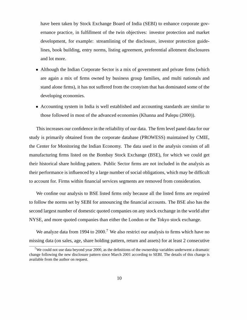
have been taken by Stock Exchange Board of India (SEBI) to enhance corporate gov-

ernance practice, in fulfillment of the twin objectives: investor protection and market

development, for example: streamlining of the disclosure, investor protection guide-

lines, book building, entry norms, listing agreement, preferential allotment disclosures

and lot more.

• Although the Indian Corporate Sector is a mix of government and private firms (which

are again a mix of firms owned by business group families, and multi nationals and

stand alone firms), it has not suffered from the cronyism that has dominated some of the

developing economies.

• Accounting system in India is well established and accounting standards are similar to

those followed in most of the advanced economies (Khanna and Palepu (2000)).

This increases our confidence in the reliability of our data. The firm level panel data for our

study is primarily obtained from the corporate database (PROWESS) maintained by CMIE,

the Center for Monitoring the Indian Economy. The data used in the analysis consists of all

manufacturing firms listed on the Bombay Stock Exchange (BSE), for which we could get

their historical share holding pattern. Public Sector firms are not included in the analysis as

their performance is influenced by a large number of social obligations, which may be difficult

to account for. Firms within financial services segments are removed from consideration.

We confine our analysis to BSE listed firms only because all the listed firms are required

to follow the norms set by SEBI for announcing the financial accounts. The BSE also has the

second largest number of domestic quoted companies on any stock exchange in the world after

NYSE, and more quoted companies than either the London or the Tokyo stock exchange.

We analyze data from 1994 to 2000.7 We also restrict our analysis to firms which have no

missing data (on sales, age, share holding pattern, return and assets) for at least 2 consecutive

7We could not use data beyond year 2000, as the definitions of the ownership variables underwent a dramaticchange following the new disclosure pattern since March 2001 according to SEBI. The details of this change isavailable from the author on request.

10

years8 There are 2575 firms (5224 firm years) in our sample, for which there is data required

for at least 2 consecutive years9. Our final sample consists of 2517 firms with 5,117 obser-

vations. For this unbalanced panel of 5,117 observations, we collect the following additional

data for each firm observation: advertising, distribution, depreciation, marketing, imports, ex-

ports, excise, capital and research and development (R&D) expenditure. Despite the problem

of attrition and missing data, our sample provides several distinct advantages over the samples

used in earlier studies. We perform our analysis after restricting the performance measure to

lie between 1st and 99th percentile to tackle the problem of outliers, which may be influential.

This leaves us with 5017 observations for 2478 firms.

B. Key Variables

We include four ownership variables: the managerial shareholding (director),10 institutional

investors shareholding (institutional), foreign investors shareholding (foreign), and corporate

shareholding (corporate) and their squares to examine the presence of ownership effect. The

squares of the ownership variables are included to distinguish the change in their effect after a

certain threshold. Year dummies are also included to control for contemporaneous macroeco-

nomic shocks. We use accounting measure of performance such as Return on Assets (ROA)

and Return on equity (ROE). The accounting measures do not take into account the future

prospects of firm performance but they do take into account the current status of the firm per-

formance. The share market measures of firm performance may run into severe problems,

especially in emerging market context, as most of the firms, go for debt-financing in these

economies rather than using finance from the share market. Therefore, share market measures

8We can not avoid these conditioning because we can not use firms with observations less than two continuousyears of data in our methodology.

9We drop observations, where values reported for capital stock, sales and age are missing, zero or negative10A number of studies, for example, Mork, Shleifer, and Vishny (1988) have used board of directors’ equity

holdings as a proxy for managerial ownership.

11

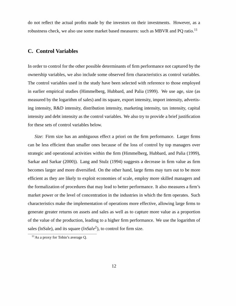
do not reflect the actual profits made by the investors on their investments. However, as a

robustness check, we also use some market based measures: such as MBVR and PQ ratio.11

C. Control Variables

In order to control for the other possible determinants of firm performance not captured by the

ownership variables, we also include some observed firm characteristics as control variables.

The control variables used in the study have been selected with reference to those employed

in earlier empirical studies (Himmelberg, Hubbard, and Palia (1999). We use age, size (as

measured by the logarithm of sales) and its square, export intensity, import intensity, advertis-

ing intensity, R&D intensity, distribution intensity, marketing intensity, tax intensity, capital

intensity and debt intensity as the control variables. We also try to provide a brief justification

for these sets of control variables below.

Size: Firm size has an ambiguous effect a priori on the firm performance. Larger firms

can be less efficient than smaller ones because of the loss of control by top managers over

strategic and operational activities within the firm (Himmelberg, Hubbard, and Palia (1999),

Sarkar and Sarkar (2000)). Lang and Stulz (1994) suggests a decrease in firm value as firm

becomes larger and more diversified. On the other hand, large firms may turn out to be more

efficient as they are likely to exploit economies of scale, employ more skilled managers and

the formalization of procedures that may lead to better performance. It also measures a firm’s

market power or the level of concentration in the industries in which the firm operates. Such

characteristics make the implementation of operations more effective, allowing large firms to

generate greater returns on assets and sales as well as to capture more value as a proportion

of the value of the production, leading to a higher firm performance. We use the logarithm of

sales (lnSale), and its square (lnSale2), to control for firm size.

11As a proxy for Tobin’s average Q.

12

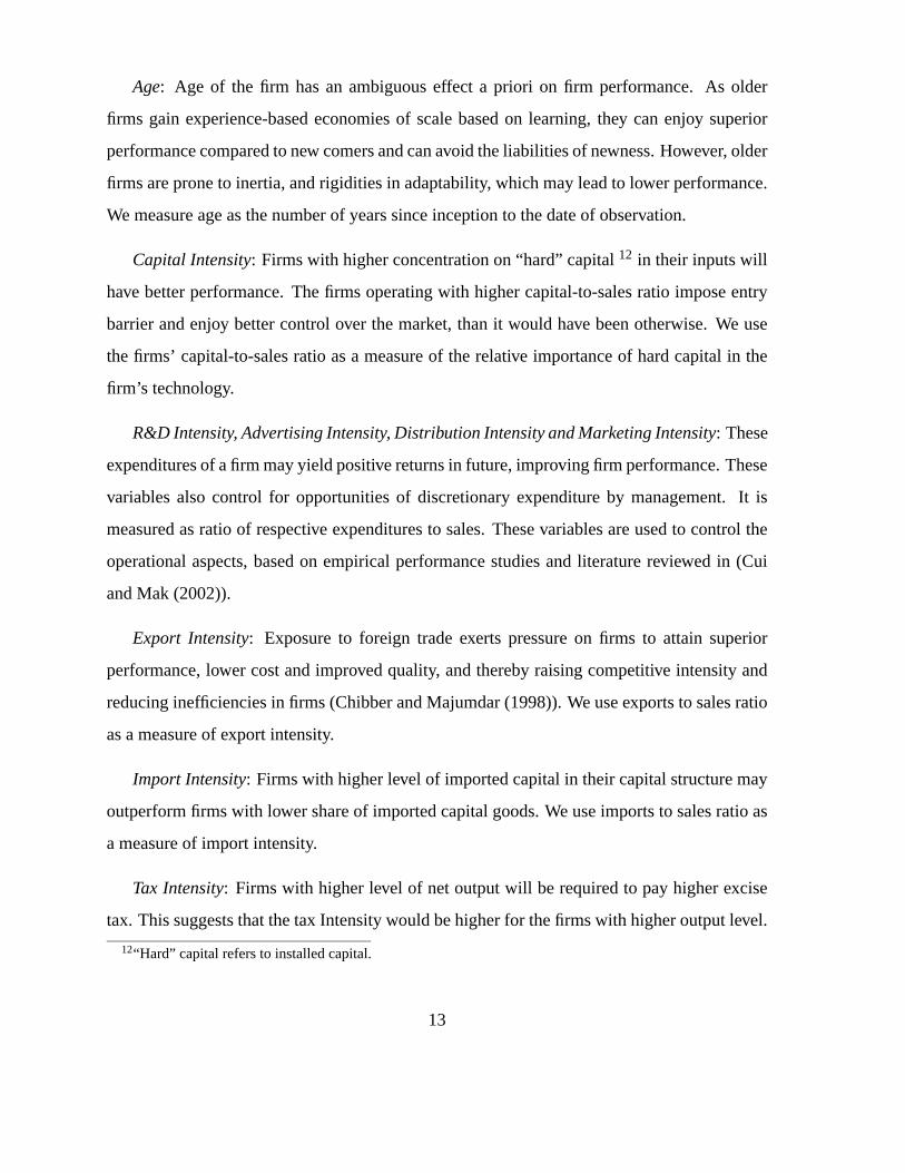
Age: Age of the firm has an ambiguous effect a priori on firm performance. As older

firms gain experience-based economies of scale based on learning, they can enjoy superior

performance compared to new comers and can avoid the liabilities of newness. However, older

firms are prone to inertia, and rigidities in adaptability, which may lead to lower performance.

We measure age as the number of years since inception to the date of observation.

Capital Intensity: Firms with higher concentration on “hard” capital12 in their inputs will

have better performance. The firms operating with higher capital-to-sales ratio impose entry

barrier and enjoy better control over the market, than it would have been otherwise. We use

the firms’ capital-to-sales ratio as a measure of the relative importance of hard capital in the

firm’s technology.

R&D Intensity, Advertising Intensity, Distribution Intensity and Marketing Intensity: These

expenditures of a firm may yield positive returns in future, improving firm performance. These

variables also control for opportunities of discretionary expenditure by management. It is

measured as ratio of respective expenditures to sales. These variables are used to control the

operational aspects, based on empirical performance studies and literature reviewed in (Cui

and Mak (2002)).

Export Intensity: Exposure to foreign trade exerts pressure on firms to attain superior

performance, lower cost and improved quality, and thereby raising competitive intensity and

reducing inefficiencies in firms (Chibber and Majumdar (1998)). We use exports to sales ratio

as a measure of export intensity.

Import Intensity: Firms with higher level of imported capital in their capital structure may

outperform firms with lower share of imported capital goods. We use imports to sales ratio as

a measure of import intensity.

Tax Intensity: Firms with higher level of net output will be required to pay higher excise

tax. This suggests that the tax Intensity would be higher for the firms with higher output level.

12“Hard” capital refers to installed capital.

13

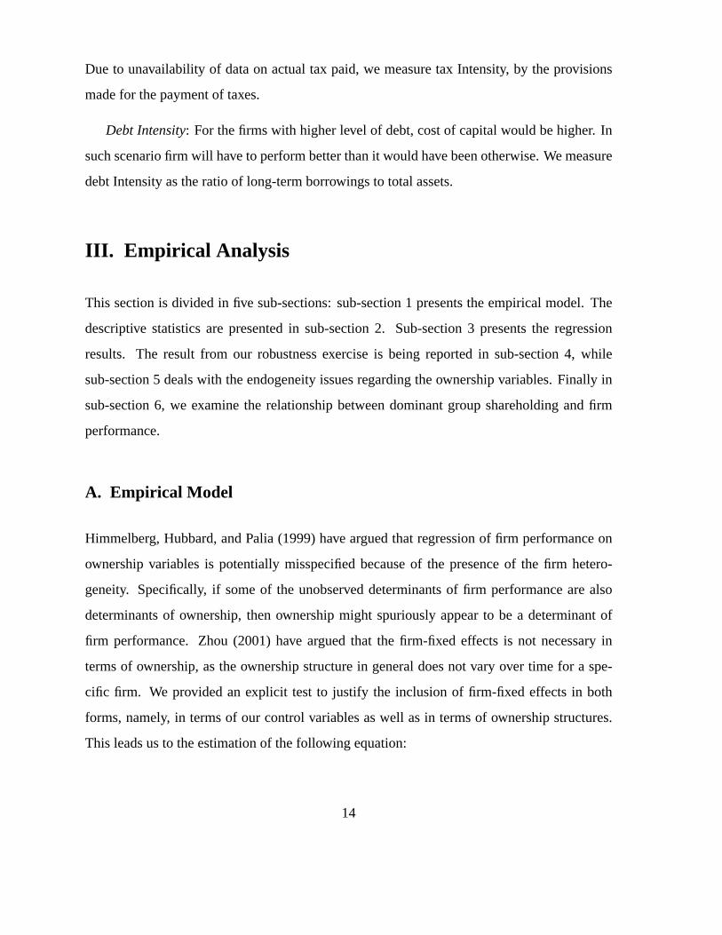
Due to unavailability of data on actual tax paid, we measure tax Intensity, by the provisions

made for the payment of taxes.

Debt Intensity: For the firms with higher level of debt, cost of capital would be higher. In

such scenario firm will have to perform better than it would have been otherwise. We measure

debt Intensity as the ratio of long-term borrowings to total assets.

III. Empirical Analysis

This section is divided in five sub-sections: sub-section 1 presents the empirical model. The

descriptive statistics are presented in sub-section 2. Sub-section 3 presents the regression

results. The result from our robustness exercise is being reported in sub-section 4, while

sub-section 5 deals with the endogeneity issues regarding the ownership variables. Finally in

sub-section 6, we examine the relationship between dominant group shareholding and firm

performance.

A. Empirical Model

Himmelberg, Hubbard, and Palia (1999) have argued that regression of firm performance on

ownership variables is potentially misspecified because of the presence of the firm hetero-

geneity. Specifically, if some of the unobserved determinants of firm performance are also

determinants of ownership, then ownership might spuriously appear to be a determinant of

firm performance. Zhou (2001) have argued that the firm-fixed effects is not necessary in

terms of ownership, as the ownership structure in general does not vary over time for a spe-

cific firm. We provided an explicit test to justify the inclusion of firm-fixed effects in both

forms, namely, in terms of our control variables as well as in terms of ownership structures.

This leads us to the estimation of the following equation:

14

Performanceit = f ( Foreignit , Institutional it , Corporateit , Director it , lnSaleit , Ageit ,

DebtInt .it , Exp.Int .it , Imp .Int .it , R&DInt .it , Adv.Int .it , Dis.Int .it ,

Cap.Int .it , Mkt .Int .it )+ δi + γt + εit (1)

where i and t represent the firm and periods, respectively,δi is the firm-specific effect, andεit

is the error term.

Performanceit = α + β(Ownership)it + γX it + θt + δi + εit (2)

where(Ownership)it variables measures the fraction of the equity of firm i, lying between 0

and 100, that is owned by different group of owners in period t. TheXit variables are firm-

specific factors. This specification allows for a firm specific fixed effectδi , time effects which

are common to firms captured by year dummies (θt), and a random unobserved component

εit . The main advantage of a fixed effect estimation model is that it would control for the

selection biases (see Gupta (2001)). Percentage shareholding of different investors (Foreign,

Institutional, Corporate and Director) are correlated, because, these shares, along with the

shares of ‘other top 50 shareholders’ and ‘others not included above’ adds upto ‘100’ percent.

In order to avoid the problem of multi- collinearity, we use only four main shareholders, i.e.

foreign, institutional, corporate, and director. We also use 1-digit and 2-digit level industry

dummies, based on industrial classification of Annual Survey of Industries-National Industrial

Classification’ (1998) by NSSO (National Sample Survey Organization), which has similar

classification as of Standard Industrial Classification (SIC).

15

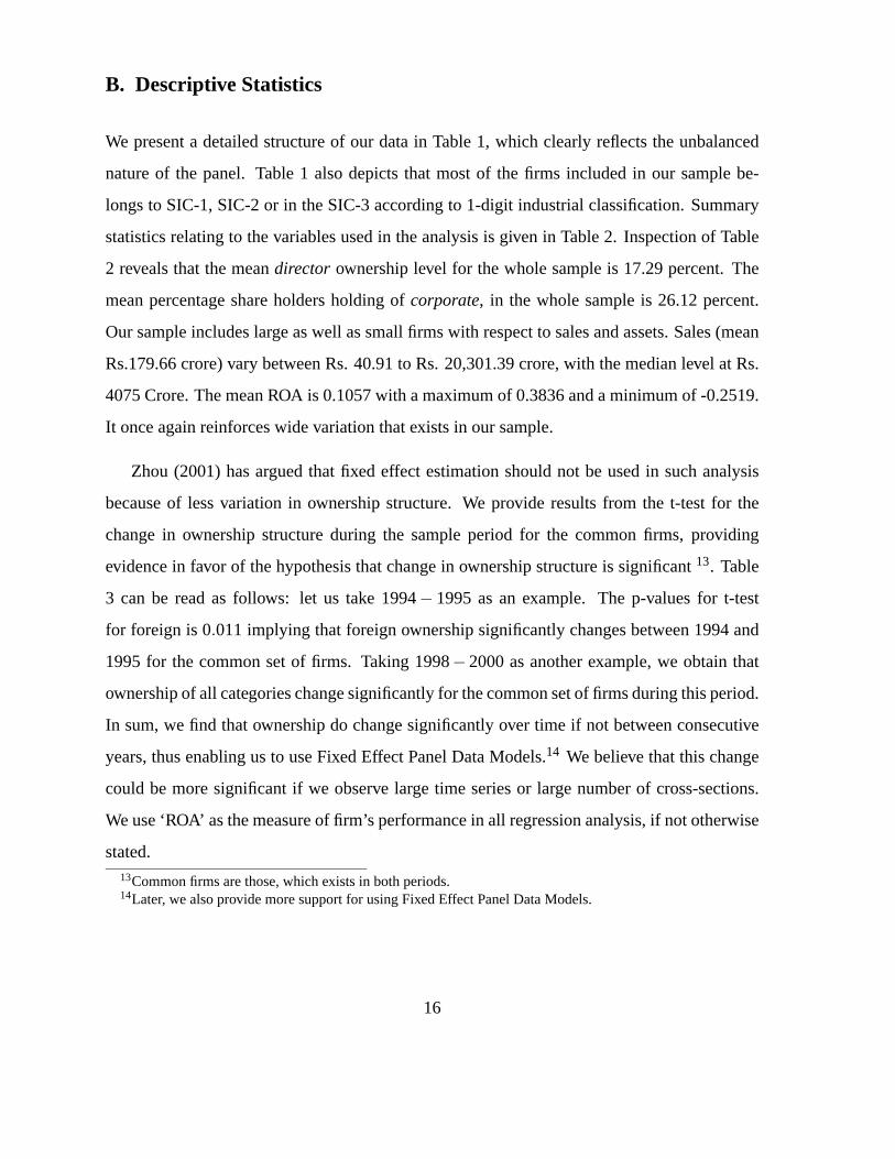
B. Descriptive Statistics

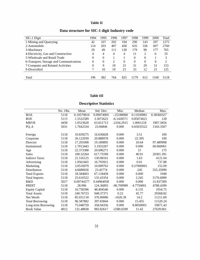
We present a detailed structure of our data in Table 1, which clearly reflects the unbalanced

nature of the panel. Table 1 also depicts that most of the firms included in our sample be-

longs to SIC-1, SIC-2 or in the SIC-3 according to 1-digit industrial classification. Summary

statistics relating to the variables used in the analysis is given in Table 2. Inspection of Table

2 reveals that the meandirector ownership level for the whole sample is 17.29 percent. The

mean percentage share holders holding ofcorporate, in the whole sample is 26.12 percent.

Our sample includes large as well as small firms with respect to sales and assets. Sales (mean

Rs.179.66 crore) vary between Rs. 40.91 to Rs. 20,301.39 crore, with the median level at Rs.

4075 Crore. The mean ROA is 0.1057 with a maximum of 0.3836 and a minimum of -0.2519.

It once again reinforces wide variation that exists in our sample.

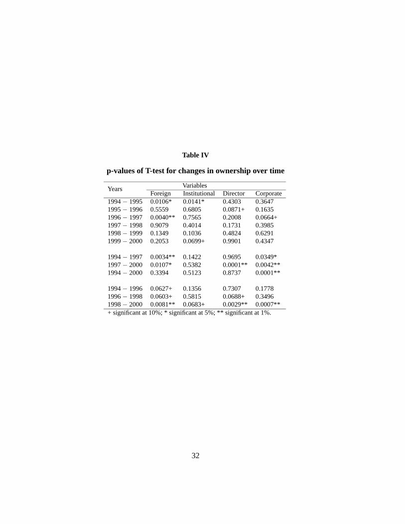
Zhou (2001) has argued that fixed effect estimation should not be used in such analysis

because of less variation in ownership structure. We provide results from the t-test for the

change in ownership structure during the sample period for the common firms, providing

evidence in favor of the hypothesis that change in ownership structure is significant13. Table

3 can be read as follows: let us take 1994− 1995 as an example. The p-values for t-test

for foreign is 0.011 implying that foreign ownership significantly changes between 1994 and

1995 for the common set of firms. Taking 1998−2000 as another example, we obtain that

ownership of all categories change significantly for the common set of firms during this period.

In sum, we find that ownership do change significantly over time if not between consecutive

years, thus enabling us to use Fixed Effect Panel Data Models.14 We believe that this change

could be more significant if we observe large time series or large number of cross-sections.

We use ‘ROA’ as the measure of firm’s performance in all regression analysis, if not otherwise

stated.13Common firms are those, which exists in both periods.14Later, we also provide more support for using Fixed Effect Panel Data Models.

16

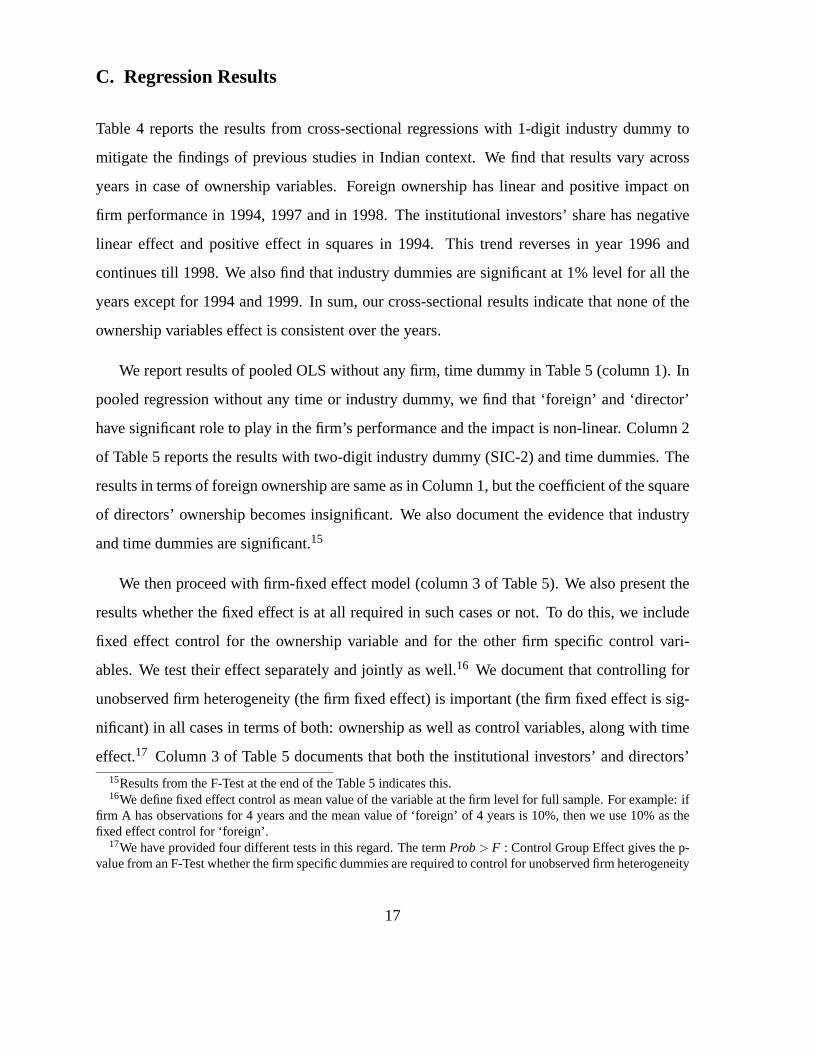
C. Regression Results

Table 4 reports the results from cross-sectional regressions with 1-digit industry dummy to

mitigate the findings of previous studies in Indian context. We find that results vary across

years in case of ownership variables. Foreign ownership has linear and positive impact on

firm performance in 1994, 1997 and in 1998. The institutional investors’ share has negative

linear effect and positive effect in squares in 1994. This trend reverses in year 1996 and

continues till 1998. We also find that industry dummies are significant at 1% level for all the

years except for 1994 and 1999. In sum, our cross-sectional results indicate that none of the

ownership variables effect is consistent over the years.

We report results of pooled OLS without any firm, time dummy in Table 5 (column 1). In

pooled regression without any time or industry dummy, we find that ‘foreign’ and ‘director’

have significant role to play in the firm’s performance and the impact is non-linear. Column 2

of Table 5 reports the results with two-digit industry dummy (SIC-2) and time dummies. The

results in terms of foreign ownership are same as in Column 1, but the coefficient of the square

of directors’ ownership becomes insignificant. We also document the evidence that industry

and time dummies are significant.15

We then proceed with firm-fixed effect model (column 3 of Table 5). We also present the

results whether the fixed effect is at all required in such cases or not. To do this, we include

fixed effect control for the ownership variable and for the other firm specific control vari-

ables. We test their effect separately and jointly as well.16 We document that controlling for

unobserved firm heterogeneity (the firm fixed effect) is important (the firm fixed effect is sig-

nificant) in all cases in terms of both: ownership as well as control variables, along with time

effect.17 Column 3 of Table 5 documents that both the institutional investors’ and directors’15Results from the F-Test at the end of the Table 5 indicates this.16We define fixed effect control as mean value of the variable at the firm level for full sample. For example: if

firm A has observations for 4 years and the mean value of ‘foreign’ of 4 years is 10%, then we use 10% as thefixed effect control for ‘foreign’.

17We have provided four different tests in this regard. The termProb> F : Control Group Effect gives the p-value from an F-Test whether the firm specific dummies are required to control for unobserved firm heterogeneity

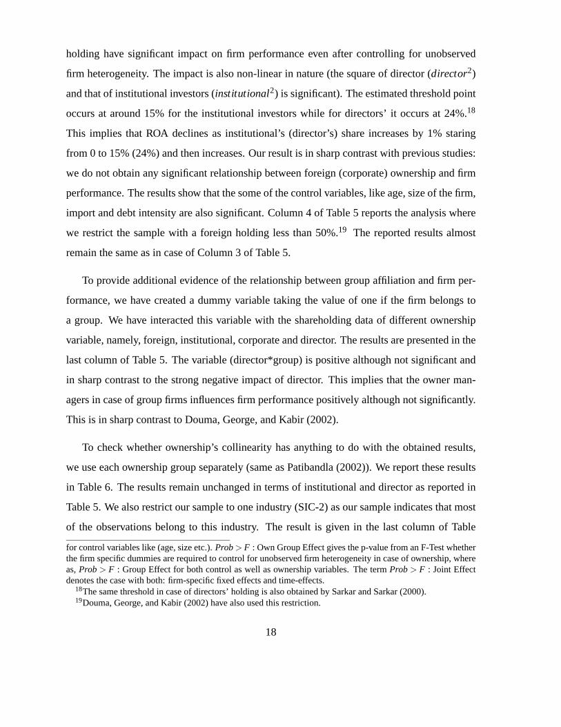
17

holding have significant impact on firm performance even after controlling for unobserved

firm heterogeneity. The impact is also non-linear in nature (the square of director (director2)

and that of institutional investors (institutional2) is significant). The estimated threshold point

occurs at around 15% for the institutional investors while for directors’ it occurs at 24%.18

This implies that ROA declines as institutional’s (director’s) share increases by 1% staring

from 0 to 15% (24%) and then increases. Our result is in sharp contrast with previous studies:

we do not obtain any significant relationship between foreign (corporate) ownership and firm

performance. The results show that the some of the control variables, like age, size of the firm,

import and debt intensity are also significant. Column 4 of Table 5 reports the analysis where

we restrict the sample with a foreign holding less than 50%.19 The reported results almost

remain the same as in case of Column 3 of Table 5.

To provide additional evidence of the relationship between group affiliation and firm per-

formance, we have created a dummy variable taking the value of one if the firm belongs to

a group. We have interacted this variable with the shareholding data of different ownership

variable, namely, foreign, institutional, corporate and director. The results are presented in the

last column of Table 5. The variable (director*group) is positive although not significant and

in sharp contrast to the strong negative impact of director. This implies that the owner man-

agers in case of group firms influences firm performance positively although not significantly.

This is in sharp contrast to Douma, George, and Kabir (2002).

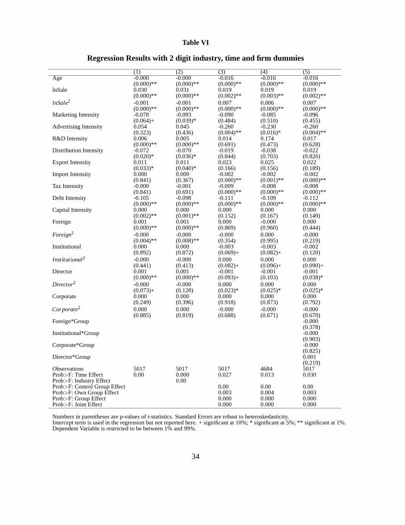
To check whether ownership’s collinearity has anything to do with the obtained results,

we use each ownership group separately (same as Patibandla (2002)). We report these results

in Table 6. The results remain unchanged in terms of institutional and director as reported in

Table 5. We also restrict our sample to one industry (SIC-2) as our sample indicates that most

of the observations belong to this industry. The result is given in the last column of Table

for control variables like (age, size etc.).Prob> F : Own Group Effect gives the p-value from an F-Test whetherthe firm specific dummies are required to control for unobserved firm heterogeneity in case of ownership, whereas,Prob> F : Group Effect for both control as well as ownership variables. The termProb> F : Joint Effectdenotes the case with both: firm-specific fixed effects and time-effects.

18The same threshold in case of directors’ holding is also obtained by Sarkar and Sarkar (2000).19Douma, George, and Kabir (2002) have also used this restriction.

18

6. We, however, include the entire ownership category in this case. In this case, although,

‘institutional’ still continues to be significant, ‘director’ looses its significance.

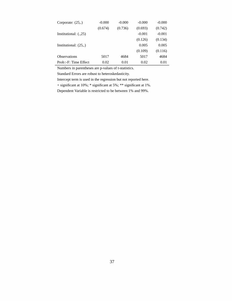
To focus more on the obtained results, we also use two different specifications by estimat-

ing the spline specification in terms of ownership variable in the regression. The first one in-

cludes two piece-wise linear terms in ownership variables (‘foreign1’, ‘foreign2’, ‘director1’,

‘director2’, ‘institutional1’, ‘institutional2’, and ‘corporate1’, ‘corporate2’.) Specifically,

Foreign1 =

foreign ownership level if foreign ownership level< 25,

25 everywhere else;

Foreign2 =

0 if foreign ownership level< 25,

foreign ownership level minus 25 if foreign ownership level≥ 25.

Similarly we specify piece-wise linear terms for (‘director’) and (‘corporate’), but in case

of (‘institutional’) we use 15%.20 In second specification we include again two piece- wise

linear terms in ownership variables (‘Foreign1’, ‘Foreign2’, ‘Director1’, ‘Director2’, ‘Institu-

tional1’, ‘Institutional2’, and ‘Corporate1’, ‘Corporate2’.) However, here we use 25% of all

four categories.

The result with the spline estimation is reported in Table 7. Column 1 of Table 7 reports the

case with first spline, where as in column 3, we report the case with the second one. In column

2 of Table 7, the result with the first spline specification is reported for those firms where the

foreign ownership is less than 50%. The estimates from column 1 show that ROA significantly

increases by 0.7% for every 1% increase in directors’ holdings after 25% and significantly

decreases by 0.2% for every 1% increase in institutional investors’ holdings below 15%. Use

of threshold points at 25% for the spline does not alter the results, except that institutional and

its square is marginally insignificant (column 4 of Table 7).

20Recall that from our regression results of column 2 (Table 5), we obtain 15% as the threshold point in caseof ‘Institutional’.

19

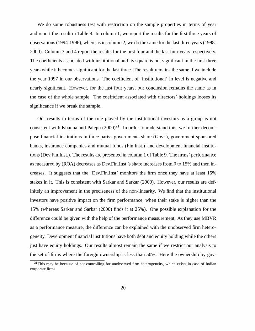
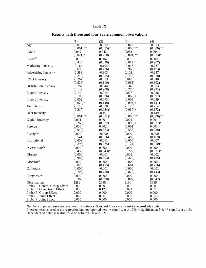
We do some robustness test with restriction on the sample properties in terms of year

and report the result in Table 8. In column 1, we report the results for the first three years of

observations (1994-1996), where as in column 2, we do the same for the last three years (1998-

2000). Column 3 and 4 report the results for the first four and the last four years respectively.

The coefficients associated with institutional and its square is not significant in the first three

years while it becomes significant for the last three. The result remains the same if we include

the year 1997 in our observations. The coefficient of ‘institutional’ in level is negative and

nearly significant. However, for the last four years, our conclusion remains the same as in

the case of the whole sample. The coefficient associated with directors’ holdings looses its

significance if we break the sample.

Our results in terms of the role played by the institutional investors as a group is not

consistent with Khanna and Palepu (2000)21. In order to understand this, we further decom-

pose financial institutions in three parts: governments share (Govt.), government sponsored

banks, insurance companies and mutual funds (Fin.Inst.) and development financial institu-

tions (Dev.Fin.Inst.). The results are presented in column 1 of Table 9. The firms’ performance

as measured by (ROA) decreases as Dev.Fin.Inst.’s share increases from 0 to 15% and then in-

creases. It suggests that the ‘Dev.Fin.Inst’ monitors the firm once they have at least 15%

stakes in it. This is consistent with Sarkar and Sarkar (2000). However, our results are def-

initely an improvement in the preciseness of the non-linearity. We find that the institutional

investors have positive impact on the firm performance, when their stake is higher than the

15% (whereas Sarkar and Sarkar (2000) finds it at 25%). One possible explanation for the

difference could be given with the help of the performance measurement. As they use MBVR

as a performance measure, the difference can be explained with the unobserved firm hetero-

geneity. Development financial institutions have both debt and equity holding while the others

just have equity holdings. Our results almost remain the same if we restrict our analysis to

the set of firms where the foreign ownership is less than 50%. Here the ownership by gov-

21This may be because of not controlling for unobserved firm heterogeneity, which exists in case of Indiancorporate firms

20

ernment sponsored banks, insurance companies and mutual funds becomes also significant in

influencing firm performance if their ownership crosses 19%.

D. Robustness of the Results

To check the robustness of our results, we report some further findings in Table 10. In column

1, firms with positive ROA are considered for the regression analysis. The results indicate

that except institutional, none of the other ownership variables are significant. The same

feature holds true for firms with firms having a manufacturing intensity higher than 50%,

although the square of the directors’ shareholding significantly increases performance of the

firms (column 3). Performance of firms with positive net worth does not share a significant

relationship with ownership (column 2). In column 5, we report the case for top 25% firms

according to gross sales and bottom 25% in column 6. We find that performance of firms in

top 25% class or in bottom 25% class does not change with change in ownership structure,

but their performance does change for top 25% of the firms classified by age variable with the

ownership of institutional investors (column 7).

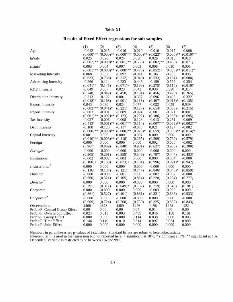
We have stated earlier that to mitigate the problem of outliers, we restrict the dependent

variable (ROA) to lie between 1% and 99%. We test the sensitivity of this by restricting ROA

to lie between 10% and 90%. Column 1 of Table 11 reports the results. We still find the

institutional is significant in level and also in its square, however, the variable director looses

its significance. The threshold point for institutional is found to be at 18%. It implies that ROA

decreases when institutional increases upto 18% and then starts increasing. Omitting firms

where foreign ownership is more than 50% does not alter our results (column 2 of Table 11).

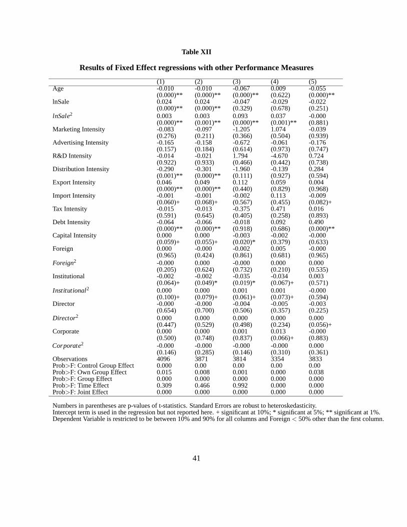
We also perform our analysis in terms of other performance variable: Return on Equity (ROE),

Market to Book value ratio (MBVR) and PQ ratio (PQA). In all these cases, we restrict the

dependent variable to lie between 10% and 90% and we impose the additional restriction that

foreign ownership (‘foreign’) to be less than 50%. When we use ROE as dependent variable,

‘institutional’ still has negative effect on firm performance in level and positive effect with its

21

squares, which is similar with ROA as performance measure. The threshold point turns out to

be at 19% in case of ROE.22 Use of market based measure such as MBVR does not change the

results in terms of institutional ownership, however, here the holding by corporates’ increases

firm value in level.23 The last column of Table 11 reports the result where we PQA as our

performance. In this case, we find that only the directors’ holding increases the value of the

firm if the directors’ holding crosses 18%.

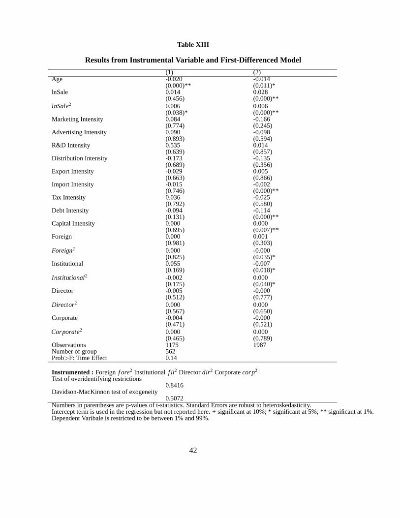
E. Is Ownership Endogenous?

There has been increasing concern about the endogeneity issue of ownership variables in liter-

ature Himmelberg, Hubbard, and Palia (1999). We try to mitigate this problem in this part of

our paper. The results are given in Table 12. Column 2 of Table 12 reports the results where

we use 2nd lag and the difference between 1st and 2nd lag of the ownership variable as instru-

ments. Results from the endogeneity and over-identification test are reported in Table 12. We

find that ownership variables are not endogenous. We also document that use of instruments

satisfies the over-identification test. In the last column of Table 12, we also report the results

from the first-differenced model.24 Our results document that changes in institutional investors

influences the changes in firm performance significantly and the effect is non-linear. Here the

directors’ shareholding is no longer significant. We also show that if the foreign ownership

increases over 13%, then the changes in foreign ownership exerts a negative influence on firm

performance.

22Restricting ROE to lie between 1% and 99% does not alter our results. The results are not presented althoughavailable on request.

23Without restriction on foreign ownership gives the same qualitative result in case of MBVR as reported inTable 11. However, if we restrict MBVR to lie between 1% and 99%, ownership variable is not significant ininfluencing MBVR.

24First-differencing is another approach to remove the fixed effects.

22

F. Does the Dominant Owner Influences Performance?

In order to examine whether the dominant owner influences firm performance, we construct

a variable that acts as a proxy for the dominant shareholding equity of an owner group. For

each observation, we use the maximum of the shareholding of the four owners as the dominant

ones. We use that shareholding representing the stake of the dominant group and use zeros for

the others.25 To be consistent with our previous specification, we also include the square of

the shareholding by the dominant owner. The results are reported in Table 14. We obtain that

if the directors’ act as a dominant group, it influences firm performance even after controlling

for unobserved firm heterogeneity. The impact is non-linear in nature (although the level is

not significant, the square term is significant). The estimated threshold point occurs at around

21%.

IV. Conclusion

This study has examined empirically the relationship between the ownership structure and

firm performance using a panel of Indian corporate firms over 1994-2000. We document

that unobserved firm heterogeneity explains a large fraction of cross-sectional variation in

shareholding pattern that exists among Indian corporate firms.

We conclude that the foreign shareholding pattern does not influence the firm performance

significantly. This result is in sharp contrast with other existing studies with respect to India

and other developing countries, which find that foreign ownership lead to higher performance.

We document that institutional investors especially the development financial institutions af-

fect firm performance positively once their ownership crosses a threshold level. Financial

institutions monitor the firm once they have at least 15% equity stakes in it. The sharehold-

25For example, for firm i in year t, suppose that the holdings by the foreign, institutional, corporates’ anddirectors’ stand at 16%, 4%, 12% and 27% respectively. In our construction, we would classify the directors’ asthe dominant group with a shareholding of 27% and the rest as zero.

23

ing by the directors’ also influences the performance of the firm beyond a certain threshold.

This is consistent with the fact that many Indian corporates’ are family dominated enterprises.

Our analysis also document that the effect of managerial shareholding and firm performance

does not differ significantly across group and stand-alone firms. Our results also document

that ownership variable is not endogenous. Given the contradictory results produced by the

current study and the prior studies using Indian data, it is clear that there are many questions

relating to the relationship between share holding pattern and performance of the firm, which

remain unsolved. There remains the task of finding out the mechanisms for the determination

of shareholding pattern and corporate governance practices. One other useful extension of

this analysis would be to include additional policy variables measuring changes in the market

conditions such as trade or tax policy changes, to see whether ownership structure changes

dramatically or not, if so to what extent and why? Do companies in emerging markets actu-

ally raise substantial equity finance? Who are the buyers of this equity? If they are dispersed

minority shareholder, why are they buying equity despite the apparent absence of minority

protections? However, these are left for future research.

24

References

Agrawal, A., and C. Knober, 1996, Firm performance and mechanisms to control agency problems

between managers and shareholders,Journal of Financial and Quantitative Analysis31, 377–397.

Ahuja, Gautam, and Sumit K. Majumdar, 1998, An Assessment of the Performance of Indian State-

Owned Enterprises,The Journal of Productivity Analysis9, 113–132.

Barbosa, Natalia, and Helen Louri, 2002, On The Determinants of Multinationals’ Ownership Pref-

erences: Evidence from Greece and Portugal,International Journal of Industrial Economics20,

493–515.

Berle, Adolf A., and Gardiner C. Means, 1932,The Modern Corporation and Private Property. (Lar-

court, Brace & World Inc. New York (Republished:1968)).

Chen, Carl R., Weiyu Guo, and Vivek Mande, 2003, Managerial ownership and firm valuation : Evi-

dence from Japanese firms,Pacific-Basin Finance Journal11, 267–283.

Chibber, Pradeep K., and Sumit K. Majumdar, 1998, State as Investor and State as Owner: Con-

sequences for Firm Performance in India,Economic Development and Cultural Change46,no.3,

561–580.

Chibber, Pradeep K., and Sumit K. Majumdar, 1999, Foreign Ownership and Profitability: Property

Rights, Control, and the Performance of Firms in Indian Industry,The Journal of Law and Eco-

nomicsXLII, 209–238.

Claessens, Stijn, Simeon Djankov, and Larry H. P. Lang, 2000, The Separation of Ownership and

Control in East Asian Corporations,The Journal of Financial Economics58, 81–112.

Claessens, Stijn, and Joseph P. H. Fan, 2003, Corporate Governance in Asia: A Survey,International

Review of Finance3(2), 71–113.

Coase, Ronald, 1960, The Problem of Social Cost,The Journal of Law and Economics1, 1–44.

Cui, Huimin, and Y. T. Mak, 2002, The relationship between Managerial Ownership and Firm Perfor-

mance in High R&D Firms,Journal of Corporate Finance8, 313–336.

25

Douma, Sytse, Rejie George, and Rezaul Kabir, 2002, Foreign and Domestic Ownership, Business

Groups and Firm Performance: Evidence from a Large Emerging Market, Titenburg University

Working Paper.

Fama, Eugene F., and Michael C. Jensen, 1983, Separation of Ownership and Control,The Journal of

Law and Economics26, 301–325.

Gupta, Nandini, 2001, Partial Privatization and Firm Performance, William Davidson Institute Working

Paper:426.

Hart, Oliver D., 1983, The Market Mechanism as an Incentive Scheme,The Bell Journal of Economics

14(2), 366–382.

Himmelberg, Charles P., R. Glenn Hubbard, and Darius Palia, 1999, Understanding the Determinants of

Managerial Ownership and the Link Between Ownership and Performance,The Journal of Financial

Economics53, 353–384.

Jensen, Michael C., 1986, Agency Costs of Free Cash Flow, Corporate Finance, and Takeovers,AEA

Papers and Proceedings76(2), 323–329.

Jensen, Michael C., and William H. Meckling, 1976, Theory of the Firm: Managerial Behavior, Agency

Costs and Ownership Structure,The Journal of Financial Economics3, 305–360.

Jensen, Michael C., and K. J. Mourphy, 1990, Performance pay and top management incentive,Journal

of Political Economics98, 225–264.

Jensen, Michael C., and J. Warner, 1988, The distribution of Power among corporate managers, share-

holders, and directors,The Journal of Financial Economics20, 3–24.

Kar, Pratip, 2001, Corporate Governance in India, inCorporate Governance in Asia - A Comparative

Perspective(OECD, OECD ).

Khanna, Tarun, and Krishna Palepu, 2000, Is Group Affiliation Profitable in Emerging Markets? An

Analysis of Diversified Indian Business Groups,The Journal of FinanceLV,no.2, 867–891.

Lang, Larry H. P., and Rane M. Stulz, 1994, Tobin’s q, Corporate Diversification and Firm Perfor-

mance,Journal of Political Economics102,no.6, 1248–1280.

26

Majumdar, Sumit K., 1998, Capital Structure and Performance: Evidence from a transition economy

on an aspect of Corporate Governance,Public Choice98, 287–305.

McConnell, John J., and Henri Servaes, 1990, Additional Evidence on Equity Ownership and Corporate

Value,The Journal of Financial Economics27, 595–612.

Megginson, William L., and Jeffery M. Netter, 2001, From State to Market: A Survey of Empirical

Studies on Privatization,Journal of Economic LiteratureXXXIX, 321–389.

Mork, Randall, Andrei Shleifer, and Robert W. Vishny, 1988, Management Ownership and Market

Valuation - An Empirical Analysis,The Journal of Financial Economics20, 293–315.

Patibandla, Murali, 2002, Equity Pattern, Corporate Governance and Performance: A Study of Indian

corporate Sector, Copenhagen Business School, Working Paper.

Porta, Rafel La, Florencio Lopez-De-Silanes, and Andrei Shleifer, 1999, Corporate Ownership Around

the World,The Journal of FinanceLIV, No.2, 471–517.

Qi, Daqing, Woody Wu, and Hua Zhang, 2000, Shareholding structure and corporate performance of

partially privatized firms: Evidence from listed Chinese companies,Pacific-Basin Finance Journal

8, 587–610.

Sarkar, Jayati, and Subrata Sarkar, 2000, Large Shareholder Activism in Corporate Governance in

Developing Countries: Evidence From India,International Review of Finance1,no.3, 161–194.

Shleifer, Andrei, and Robert W. Vishny, 1986, Large Shareholders and Corporate Control,Journal of

Political Economics94,no.3, 461–488.

Shleifer, Andrei, and Robert W. Vishny, 1997, A Survey of Corporate Governance,The Journal of

FinanceLII,no.2, 737–783.

Short, Helen, 1994, Ownership, Control, Financial Structure and the Performance of Firms,Journal of

Economic Surveys8,no.3, 203–209.

Wiwattanakantang, Yupana, 2001, Controlling shareholders and corporate value: Evidence from Thai-

land,Pacific-Basin Finance Journal9, 323–362.

27

Zhou, Xianming, 2001, Understanding the determinants of managerial ownership and the link between

ownership and performance: comment,The Journal of Financial Economics62, 559–571.

28

Table I: List of Variables

Abbreviation Description

Performance Measures: ROA, ROE, MBVR, PQA

ROA We measure Return on Assets as the ratio of return to total assets, where re-

turn is defined as the difference between operating revenues and expenditure

before tax and interest payments (i.e. pbdit) and total asset of firm includes

fixed assets, investments and current assets. R&D expenditures are included in

operating expenditure in the year incurred, even though the R&D results may

produce technical breakthroughs that will benefit the firm for years to come.

We treat, therefore, R&D as investment rather than as current expenditure. To-

tal assets include value of fixed assets, investments and current assets.

ROA = Profit Before Depriciation, Interest and Tax (PBDIT) / Total Assets

ROE We measure Return on Equity Capital as the ratio of return to equity capital.

Equity Capital is the total outstanding paid up equity capital of the firm as

at the end of the accounting period. Shares issued but not paid-up or pending

allotments do not form part of equity capital. This includes bonus equity shares

issued, if any, by the firm in the past.

ROE = PBDIT/ Equity Capital

PQ A Proxy for Tobin’s Average Q is defined as the ratio of the value of the firm

divided by the replacement value of firm. For firm value, we use the market

value of common equity plus total borrowings (includes all form of debt, inter-

est bearing or other wise), and for the replacement value, we use total assets.

We use last trading day’s closing price for calculating market value of the firm.

PQ A = (Total Borrowings + Market Value (Equity) )/ Total Assets

MBVR Market to Book Value Ratio is defined as the ratio of the market value of the

firm divided by the book value of firm. For market value of firm, we use the

market value of common equity plus total borrowings (includes all form of

debt, interest bearing or other wise). We use last trading day’s closing price for

calculating market value of the firm.

MBVR = (Total Borrowings + Market Value (Equity) )/ Book Value (Equity)

Ownership Variables

Foreign Foreigners’ Share Holding is equity shares held by foreigners as percentage

of total equity shares. These include foreign collaborators, foreign financial

institutions, foreign nationals and non-resident Indians.

Institutional Governments’ and Financial Institutions’ Share Holding is equity shares held

by government companies as percentage of total equity shares. These includes

insurance companies, mutual funds, financial institutions, banks, central and

state government firms, state financial Corporations and other government bod-

ies.

Corporate Corporates’ Share Holding is equity shares held by Corporate bodies as a per-

centage of total equity shares. These include corporate bodies excluding those

already covered.

29

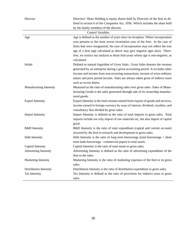
Director Directors’ Share Holding is equity shares held by Directors of the firm as de-

fined in section 6 of the Companies Act, 1956. Which includes the share held

by the family members of the director.

Control Variables

Age Age is defined as the number of years since its inception. Where incorporation

year pertains to the most recent incarnation year of the firm. In the case of

firms that were reorganized, the year of incorporation may not reflect the true

age of a firm (age calculated as above may give negative ages also). There-

fore, we restrict our analysis to those firm-years whose age is non-negative, as

calculated.

lnSale Defined as natural logarithm of Gross Sales. Gross Sales denotes the revenue

generated by an enterprise during a given accounting period. It excludes other

income and income from non-recurring transactions, income of extra-ordinary

nature and prior period income. Sales are always taken gross of indirect taxes

such as excise duties.

Manufacturing Intensity Measured as the ratio of manufacturing sales over gross sales. Sales of Manu-

facturing Goods is the sales generated through sale of its ownership manufac-

tured goods.

Export Intensity Export Intensity is the total revenue earned from exports of goods and services,

income earned in foreign currency by ways of interest, dividend, royalties, and

consultancy fees divided by gross sales.

Import Intensity Import Intensity is defined as the ratio of total imports to gross sales. Total

imports include not only import of raw materials etc, but also import of capital

good.

R&D Intensity R&D Intensity is the ratio of total expenditure (capital and current account)

incurred by the firm in research and development to gross sales.

Debt Intensity Debt Intensity is the ratio of long term borrowings (total borrowings + short

term bank borrowings - commercial paper) to total assets.

Capital Intensity Capital Intensity is the ratio of total assets to gross sales.

Advertising Intensity Advertising Intensity is defined as the ratio of advertising expenditure of the

firm to the sales.

Marketing Intensity Marketing Intensity is the ratio of marketing expenses of the firm to its gross

sales.

Distribution Intensity Distribution Intensity is the ratio of distribution expenditure to gross sales.

Tax Intensity Tax Intensity is defined as the ratio of provisions for inderect taxes to gross

sales.

30

Table II

Data structure for SIC-1 digit Industry code

SIC-1 Digit 1994 1995 1996 1997 1998 1999 2000 Total1-Mining and Quarrying 42 107 202 194 290 143 297 12752-Automobile 114 203 407 458 635 336 607 27603-Machinary 29 49 111 130 179 90 177 7654-Electricity, Gas and Construction 4 4 4 4 11 2 6 355-Wholesale and Retail Trade 0 0 1 1 0 0 1 36-Transport, Storage and Communications 0 0 2 0 0 0 0 27-Computer and Related Activities 0 9 18 15 31 29 51 1539-Diversified 7 10 19 23 33 12 21 125

Total 196 382 764 825 1179 612 1160 5118

Table III

Descriptive Statistics

No. Obs. Mean Std. Dev. Min. Median Max.ROA 5118 0.10579816 0.09074905 -.25188968 0.11030981 0.38360327ROE 5115 1.5522589 3.3072623 -6.1428571 0.85074621 128MBVR 4458 1.0523628 63.651713 -2104.2915 1.0001218 1907.5856PQ A 5031 1.7642334 23.84846 0.000 0.65035522 1343.3507

Foreign 5118 10.839275 16.636828 0.000 3.51 100Corporate 5118 26.122939 20.888978 0.000 22.395 100Director 5118 17.291008 19.189895 0.000 10.64 97.489998Institutional 5118 1.7013443 5.1933267 0.000 0.000 60.060001Age 5118 22.373388 20.696271 0.000 15 175Sales 5118 180.32264 617.75599 0.000 40.91 20301.391Indirect Taxes 5118 21.516125 130.08161 0.000 1.63 4121.04Advertising 5118 1.9561665 16.793921 0.000 0.01 737.88Marketing 5118 3.0516979 10.009763 0.000 0.27000001 152.09Distribution 5118 4.6680656 23.45774 0.000 .245 555.35999Total Exports 5118 18.584603 67.118458 0.000 0.000 1948Total Imports 5118 25.610522 135.43354 0.000 2.245 5176.6899R&D 5017 0.00744277 0.44964938 0.000 0.000 31.837309PBDIT 5118 28.996 124.36893 -96.709999 4.7750001 4788.4399Equity Capital 5118 16.758396 48.404546 0.000 6.135 1054.75Total Assets 5118 240.76723 948.37371 0.22 45.77 29368.82Net Worth 5118 85.031118 376.00086 -1626.39 14.2 11211.69Total Borrowing 5118 96.587882 397.83844 0.000 15.455 11520.24Long term Borrowing 5118 75.048759 358.04356 0.000 8.8050003 10871.43Book Value 4912 131.48838 983.82617 -2580.6599 11.42 27639.061

31

Table IV

p-values of T-test for changes in ownership over time

VariablesYearsForeign Institutional Director Corporate

1994− 1995 0.0106* 0.0141* 0.4303 0.36471995− 1996 0.5559 0.6805 0.0871+ 0.16351996− 1997 0.0040** 0.7565 0.2008 0.0664+1997− 1998 0.9079 0.4014 0.1731 0.39851998− 1999 0.1349 0.1036 0.4824 0.62911999− 2000 0.2053 0.0699+ 0.9901 0.4347

1994− 1997 0.0034** 0.1422 0.9695 0.0349*1997− 2000 0.0107* 0.5382 0.0001** 0.0042**1994− 2000 0.3394 0.5123 0.8737 0.0001**

1994− 1996 0.0627+ 0.1356 0.7307 0.17781996− 1998 0.0603+ 0.5815 0.0688+ 0.34961998− 2000 0.0081** 0.0683+ 0.0029** 0.0007**+ significant at 10%; * significant at 5%; ** significant at 1%.

32

Table V

Cross-sectional regression results with 1-digit industry dummy

(1) (2) (3) (4) (5) (6) (7)Age 0.000 0.000 -0.000 -0.000 -0.000 -0.000 -0.000

(0.994) (0.478) (0.108) (0.065)+ (0.000)** (0.016)* (0.044)*lnSale 0.033 0.029 0.040 0.044 0.042 0.020 0.022

(0.000)** (0.000)** (0.000)** (0.000)** (0.000)** (0.001)** (0.000)**lnSale2 -0.003 -0.003 -0.003 -0.003 -0.002 0.000 -0.000

(0.001)** (0.001)** (0.000)** (0.000)** (0.000)** (0.703) (0.373)Marketing Intensity -0.356 -0.208 -0.024 -0.104 0.033 -0.077 -0.068

(0.146) (0.164) (0.783) (0.549) (0.643) (0.525) (0.386)Advertising Intensity -0.547 -0.152 -0.015 0.212 0.285 0.428 -0.018

(0.150) (0.593) (0.863) (0.253) (0.013)* (0.007)** (0.910)R&D Intensity -0.132 2.461 -0.627 0.010 -0.073 0.006 0.058

(0.933) (0.226) (0.615) (0.975) (0.022)* (0.000)** (0.899)Distribution Intensity 0.094 0.055 0.168 0.016 -0.122 -0.056 -0.267

(0.644) (0.396) (0.036)* (0.777) (0.127) (0.529) (0.012)*Export Intensity 0.000 0.006 -0.010 -0.023 0.008 0.057 0.030

(0.993) (0.714) (0.440) (0.099)+ (0.398) (0.001)** (0.015)*Import Intensity -0.028 0.000 0.000 -0.010 -0.007 -0.035 0.001

(0.067)+ (0.731) (0.843) (0.330) (0.041)* (0.109) (0.700)Tax Intensity 0.079 0.047 0.016 0.003 0.007 0.077 -0.003

(0.265) (0.388) (0.681) (0.943) (0.563) (0.193) (0.269)Debt Intensity -0.112 -0.017 -0.087 -0.098 -0.114 -0.128 -0.090

(0.001)** (0.647) (0.000)** (0.000)** (0.000)** (0.000)** (0.000)**Capital Intensity -0.000 0.000 0.000 0.000 0.000 -0.000 -0.000

(0.750) (0.701) (0.001)** (0.000)** (0.000)** (0.625) (0.920)Foreign 0.003 0.000 0.001 0.001 0.001 0.001 0.000

(0.017)* (0.846) (0.186) (0.015)* (0.002)** (0.275) (0.296)Foreign2 -0.000 0.000 0.000 -0.000 -0.000 -0.000 -0.000

(0.372) (0.566) (0.438) (0.283) (0.035)* (0.588) (0.498)Institutional -0.004 -0.001 0.002 0.001 0.000 -0.001 -0.002

(0.099)+ (0.652) (0.096)+ (0.159) (0.954) (0.218) (0.080)+Institutional2 0.000 0.000 -0.000 -0.000 -0.000 0.000 0.000

(0.012)* (0.342) (0.074)+ (0.044)* (0.817) (0.776) (0.320)Director 0.001 0.001 0.001 0.000 0.001 0.001 0.000

(0.161) (0.181) (0.148) (0.565) (0.004)** (0.021)* (0.428)Director2 -0.000 -0.000 -0.000 0.000 -0.000 -0.000 0.000

(0.669) (0.334) (0.214) (0.802) (0.085)+ (0.102) (0.704)Corporate 0.002 -0.000 -0.000 0.000 0.000 -0.000 0.001

(0.206) (0.894) (0.974) (0.430) (0.306) (0.451) (0.165)Corporate2 -0.000 0.000 0.000 -0.000 -0.000 0.000 -0.000

(0.723) (0.734) (0.351) (0.371) (0.596) (0.097)+ (0.237)Observations 187 365 734 806 1163 600 1155Prob>F: Industry Effect 0.82 0.00 0.00 0.04 0.02 0.91 0.00

Numbers in parentheses are p-values of t-statistics. Standard Errors are robust to heteroskedasticity.Intercept term is used in the regression but not reported here. + significant at 10%; * significant at 5%; ** significant at 1%.Dependent Variable is restricted to be between 1% and 99%.

33

Table VI

Regression Results with 2 digit industry, time and firm dummies

(1) (2) (3) (4) (5)Age -0.000 -0.000 -0.016 -0.016 -0.016

(0.000)** (0.000)** (0.000)** (0.000)** (0.000)**lnSale 0.030 0.031 0.019 0.019 0.019

(0.000)** (0.000)** (0.002)** (0.003)** (0.002)**lnSale2 -0.001 -0.001 0.007 0.006 0.007

(0.000)** (0.000)** (0.000)** (0.000)** (0.000)**Marketing Intensity -0.078 -0.093 -0.090 -0.085 -0.096

(0.064)+ (0.039)* (0.484) (0.510) (0.455)Advertising Intensity 0.054 0.045 -0.260 -0.230 -0.260

(0.323) (0.436) (0.004)** (0.016)* (0.004)**R&D Intensity 0.006 0.005 0.014 0.174 0.017

(0.000)** (0.000)** (0.691) (0.473) (0.628)Distribution Intensity -0.072 -0.070 -0.019 -0.038 -0.022

(0.020)* (0.036)* (0.844) (0.703) (0.826)Export Intensity 0.011 0.011 0.023 0.025 0.022

(0.033)* (0.040)* (0.166) (0.156) (0.189)Import Intensity 0.000 0.000 -0.002 -0.002 -0.002

(0.841) (0.367) (0.000)** (0.001)** (0.000)**Tax Intensity -0.000 -0.001 -0.009 -0.008 -0.008

(0.841) (0.691) (0.000)** (0.000)** (0.000)**Debt Intensity -0.105 -0.098 -0.111 -0.109 -0.112

(0.000)** (0.000)** (0.000)** (0.000)** (0.000)**Capital Intensity 0.000 0.000 0.000 0.000 0.000

(0.002)** (0.001)** (0.152) (0.167) (0.149)Foreign 0.001 0.001 0.000 -0.000 0.000

(0.000)** (0.000)** (0.869) (0.960) (0.444)Foreign2 -0.000 -0.000 -0.000 0.000 -0.000

(0.004)** (0.008)** (0.354) (0.995) (0.219)Institutional 0.000 0.000 -0.003 -0.003 -0.002

(0.892) (0.872) (0.069)+ (0.082)+ (0.120)Institutional2 -0.000 -0.000 0.000 0.000 0.000

(0.441) (0.413) (0.082)+ (0.096)+ (0.090)+Director 0.001 0.001 -0.001 -0.001 -0.001

(0.000)** (0.000)** (0.093)+ (0.103) (0.038)*Director2 -0.000 -0.000 0.000 0.000 0.000

(0.073)+ (0.128) (0.023)* (0.025)* (0.025)*Corporate 0.000 0.000 0.000 0.000 0.000

(0.249) (0.396) (0.918) (0.873) (0.792)Corporate2 0.000 0.000 -0.000 -0.000 -0.000

(0.885) (0.819) (0.688) (0.671) (0.670)Foreign*Group -0.000

(0.378)Institutional*Group -0.000

(0.903)Corporate*Group -0.000

(0.825)Director*Group 0.001

(0.219)Observations 5017 5017 5017 4684 5017Prob>F: Time Effect 0.00 0.000 0.027 0.013 0.030Prob>F: Industry Effect 0.00Prob>F: Control Group Effect 0.00 0.00 0.00Prob>F: Own Group Effect 0.003 0.004 0.003Prob>F: Group Effect 0.000 0.000 0.000Prob>F: Joint Effect 0.000 0.000 0.000

Numbers in parentheses are p-values of t-statistics. Standard Errors are robust to heteroskedasticity.Intercept term is used in the regression but not reported here. + significant at 10%; * significant at 5%; ** significant at 1%.Dependent Variable is restricted to be between 1% and 99%.

34

Table VII

One ownership at a time with firm dummies

(1) (2) (3) (4) (5)Age -0.016 -0.016 -0.016 -0.016 -0.017

(0.000)** (0.000)** (0.000)** (0.000)** (0.000)**lnSale 0.019 0.019 0.019 0.019 0.014

(0.002)** (0.002)** (0.002)** (0.002)** (0.071)+lnSale2 0.007 0.006 0.006 0.006 0.008

(0.000)** (0.000)** (0.000)** (0.000)** (0.000)**Marketing Intensity -0.093 -0.097 -0.092 -0.091 0.040

(0.479) (0.457) (0.483) (0.486) (0.818)Advertising Intensity -0.255 -0.250 -0.247 -0.249 -0.559

(0.004)** (0.006)** (0.006)** (0.005)** (0.006)**R&D Intensity 0.015 0.007 0.011 0.012 0.010

(0.667) (0.826) (0.742) (0.731) (0.737)Distribution Intensity -0.022 -0.024 -0.025 -0.027 -0.038

(0.824) (0.804) (0.796) (0.780) (0.848)Export Intensity 0.022 0.023 0.022 0.022 0.031

(0.192) (0.177) (0.201) (0.204) (0.262)Import Intensity -0.002 -0.002 -0.002 -0.002 -0.002

(0.001)** (0.001)** (0.001)** (0.001)** (0.000)**Tax Intensity -0.009 -0.009 -0.009 -0.008 -0.011

(0.000)** (0.000)** (0.000)** (0.000)** (0.000)**Debt Intensity -0.108 -0.108 -0.106 -0.107 -0.142

(0.000)** (0.000)** (0.000)** (0.000)** (0.000)**Capital Intensity 0.000 0.000 0.000 0.000 0.000

(0.153) (0.151) (0.145) (0.147) (0.321)Foreign 0.000 0.001

(0.984) (0.202)Foreign2 -0.000 -0.000

(0.481) (0.105)Institutional -0.002 -0.003

(0.090)+ (0.082)+Institutional2 0.000 0.000

(0.095)+ (0.086)+Director -0.001 -0.001

(0.126) (0.451)Director2 0.000 0.000

(0.019)* (0.150)Corporate -0.000 -0.000

(0.872) (0.864)Corporate2 -0.000 0.000

(0.906) (0.912)Observations 5017 5017 5017 5017 2706Prob>F: Control Group Effect 0.00 0.00 0.00 0.00 0.00Prob>F: Own Group Effect 0.079 0.170 0.677 0.037 0.092Prob>F: Group Effect 0.000 0.000 0.000 0.000 0.000Prob>F: Time Effect 0.023 0.020 0.014 0.022 0.027Prob>F: Joint Effect 0.000 0.000 0.000 0.000 0.000

Numbers in parentheses are p-values of t-statistics. Standard Errors are robust to heteroskedasticity.Intercept term is used in the regression but not reported here. + significant at 10%; * significant at 5%; ** significant at 1%.Dependent Variable is restricted to be between 1% and 99%.

35

Table VIII: Spline specification with firm dummies

(1) (2) (3) (4)

Age -0.016 -0.016 -0.016 -0.016

(0.000)** (0.000)** (0.000)** (0.000)**

lnSale 0.019 0.019 0.019 0.019

(0.002)** (0.003)** (0.002)** (0.002)**

lnSale2 0.007 0.006 0.007 0.006

(0.000)** (0.000)** (0.000)** (0.000)**

Marketing Intensity -0.086 -0.082 -0.085 -0.081

(0.507) (0.527) (0.512) (0.535)

Advertising Intensity -0.260 -0.227 -0.258 -0.225

(0.004)** (0.017)* (0.004)** (0.017)*

R&D Intensity 0.010 0.176 0.010 0.172

(0.762) (0.466) (0.762) (0.473)

Distribution Intensity -0.021 -0.041 -0.021 -0.041

(0.833) (0.683) (0.830) (0.682)

Export Intensity 0.023 0.025 0.024 0.026

(0.164) (0.152) (0.161) (0.149)

Import Intensity -0.002 -0.002 -0.002 -0.002

(0.000)** (0.001)** (0.001)** (0.001)**

Tax Intensity -0.009 -0.009 -0.009 -0.009

(0.000)** (0.000)** (0.000)** (0.000)**

Debt Intensity -0.110 -0.108 -0.111 -0.109

(0.000)** (0.000)** (0.000)** (0.000)**

Capital Intensity 0.000 0.000 0.000 0.000

(0.151) (0.165) (0.150) (0.164)

Foreign: (.,25) -0.000 -0.000 -0.000 -0.000

(0.824) (0.655) (0.812) (0.640)

Foreign: (25,.) -0.001 0.001 -0.001 0.000

(0.226) (0.645) (0.237) (0.662)

Institutional: (.,15) -0.002 -0.002

(0.096)+ (0.097)+

Institutional: (15,.) 0.002 0.002

(0.155) (0.150)

Director: (.,25) -0.000 -0.000 -0.001 -0.001

(0.246) (0.259) (0.240) (0.253)

Director: (25,.) 0.001 0.001 0.001 0.001

(0.078)+ (0.086)+ (0.079)+ (0.086)+

Corporate: (.,25) -0.000 -0.000 -0.000 -0.000

(0.648) (0.630) (0.629) (0.636)

36

Corporate: (25,.) -0.000 -0.000 -0.000 -0.000

(0.674) (0.736) (0.693) (0.742)

Institutional: (.,25) -0.001 -0.001

(0.126) (0.134)

Institutional: (25,.) 0.005 0.005

(0.109) (0.116)

Observations 5017 4684 5017 4684

Prob>F: Time Effect 0.02 0.01 0.02 0.01

Numbers in parentheses are p-values of t-statistics.

Standard Errors are robust to heteroskedasticity.

Intercept term is used in the regression but not reported here.

+ significant at 10%; * significant at 5%; ** significant at 1%.

Dependent Variable is restricted to be between 1% and 99%.

37

Table IX

Results with three and four years common observations

(1) (2) (3) (4)Age -0.018 -0.012 -0.022 -0.013

(0.001)** (0.015)* (0.000)** (0.000)**lnSale 0.049 0.042 0.053 0.064

(0.021)* (0.270) (0.001)** (0.013)*lnSale2 0.002 0.004 0.005 0.000

(0.424) (0.330) (0.012)* (0.907)Marketing Intensity -0.164 -0.104 -0.013 -0.287

(0.693) (0.736) (0.965) (0.193)Advertising Intensity -0.588 -0.303 0.102 -0.247

(0.218) (0.615) (0.756) (0.218)R&D Intensity -0.267 -0.633 0.010 -0.048

(0.828) (0.110) (0.961) (0.302)Distribution Intensity -0.787 -0.044 -0.340 -0.003

(0.129) (0.900) (0.276) (0.991)Export Intensity 0.140 -0.014 0.077 -0.038

(0.109) (0.836) (0.068)+ (0.397)Import Intensity -0.002 -0.073 -0.003 -0.039

(0.020)* (0.148) (0.094)+ (0.141)Tax Intensity -0.118 -0.528 -0.178 -0.274

(0.217) (0.024)* (0.080)+ (0.172)Debt Intensity -0.170 -0.191 -0.136 -0.149

(0.001)** (0.011)* (0.000)** (0.000)**Capital Intensity 0.001 0.001 0.001 0.001

(0.265) (0.072)+ (0.093)+ (0.017)*Foreign 0.000 0.002 -0.001 0.001

(0.918) (0.374) (0.552) (0.238)Foreign2 0.000 -0.000 0.000 -0.000

(0.541) (0.356) (0.485) (0.169)Institutional -0.003 -0.011 -0.004 -0.007

(0.293) (0.075)+ (0.124) (0.050)+Institutional2 0.000 0.000 0.000 0.000

(0.455) (0.043)* (0.222) (0.031)*Director -0.000 -0.001 0.001 -0.002

(0.988) (0.603) (0.429) (0.185)Director2 0.000 0.000 -0.000 0.000

(0.820) (0.415) (0.661) (0.266)Corporate -0.000 -0.001 -0.000 -0.001

(0.705) (0.738) (0.875) (0.443)Corporate2 0.000 0.000 0.000 0.000

(0.368) (0.898) (0.807) (0.542)Observations 1282 2335 2100 3335Prob>F: Control Group Effect 0.00 0.00 0.00 0.00Prob>F: Own Group Effect 0.006 0.124 0.021 0.074Prob>F: Group Effect 0.000 0.000 0.000 0.000Prob>F: Time Effect 0.820 0.861 0.853 0.059Prob>F: Joint Effect 0.000 0.000 0.000 0.000

Numbers in parentheses are p-values of t-statistics. Standard Errors are robust to heteroskedasticity.Intercept term is used in the regression but not reported here. + significant at 10%; * significant at 5%; ** significant at 1%.Dependent Variable is restricted to be between 1% and 99%.

38

Table X

Results of Fixed Effect regression with more disagrregated ownership structure

(1) (2)Age -0.016 -0.016

(0.000)** (0.000)**lnSale 0.018 0.018

(0.007)** (0.007)**lnSale2 0.007 0.007

(0.000)** (0.000)**Marketing Intensity -0.121 -0.118

(0.354) (0.364)Advertising Intensity -0.251 -0.221

(0.007)** (0.025)*R&D Intensity 0.015 0.189

(0.674) (0.442)Distribution Intensity -0.019 -0.035

(0.851) (0.735)Export Intensity 0.035 0.036

(0.042)* (0.045)*Import Intensity -0.002 -0.002

(0.001)** (0.001)**Tax Intensity -0.009 -0.008

(0.000)** (0.000)**Debt Intensity -0.119 -0.118

(0.000)** (0.000)**Capital Intensity 0.000 0.000

(0.178) (0.177)Foreign 0.000 0.000

(0.798) (1.000)Foreign2 -0.000 0.000

(0.332) (0.966)Director -0.001 -0.001

(0.120) (0.133)Director2 0.000 0.000

(0.028)* (0.032)*Corporate 0.000 0.000

(0.849) (0.764)Corporate2 -0.000 -0.000

(0.602) (0.535)Dev. Fin. Inst. -0.003 -0.003

(0.077)+ (0.106)Dev.Fin.Inst.2 0.000 0.000

(0.081)+ (0.112)Fin. Inst. -0.001 -0.001

(0.331) (0.141)Fin.Inst.2 0.000 0.000

(0.238) (0.089)+Govt. -0.001 -0.002

(0.314) (0.205)Govt.2 0.000 0.000

(0.472) (0.470)Observations 4852 4529Prob>F: Control Group Effect 0.00 0.00Prob>F: Own Group Effect 0.021 0.019Prob>F: Group Effect 0.000 0.000Prob>F: Time Effect 0.023 0.012Prob>F: Joint Effect 0.000 0.000

Numbers in parentheses are p-values of t-statistics. Standard Errors are robust to heteroskedasticity.Intercept term is used in the regression but not reported here. + significant at 10%; * significant at 5%; ** significant at 1%.Dependent Variable is restricted to be between 10% and 90%.

39

Table XI

Results of Fixed Effect regressions for sub-samples

(1) (2) (3) (4) (5) (6) (7)Age -0.012 -0.015 -0.016 -0.010 -0.010 -0.017 -0.008

(0.000)** (0.000)** (0.000)** (0.000)** (0.023)* (0.000)** (0.010)**lnSale 0.025 0.028 0.024 0.030 0.029 -0.010 0.018

(0.002)** (0.000)** (0.001)** (0.568) (0.002)** (0.460) (0.071)+lnSale2 0.003 0.004 0.007 0.003 0.008 0.010 0.005

(0.001)** (0.000)** (0.000)** (0.470) (0.052)+ (0.000)** (0.011)*Marketing Intensity 0.068 0.037 -0.092 -0.014 0.106 -0.235 0.096

(0.633) (0.738) (0.512) (0.940) (0.533) (0.164) (0.608)Advertising Intensity -0.266 -0.114 -0.233 -0.446 -0.159 -0.599 -0.354

(0.041)* (0.145) (0.071)+ (0.193) (0.275) (0.114) (0.019)*R&D Intensity -0.049 0.007 0.023 0.043 0.030 0.320 0.317

(0.748) (0.842) (0.458) (0.784) (0.456) (0.479) (0.265)Distribution Intensity -0.313 -0.122 0.001 -0.327 -0.096 -0.483 -0.322

(0.018)* (0.168) (0.991) (0.118) (0.497) (0.013)* (0.135)Export Intensity 0.043 0.030 0.024 0.077 -0.022 0.058 0.039

(0.003)** (0.041)* (0.221) (0.127) (0.614) (0.066)+ (0.215)Import Intensity -0.003 -0.001 -0.009 -0.024 -0.001 -0.071 0.001

(0.001)** (0.002)** (0.123) (0.292) (0.106) (0.063)+ (0.695)Tax Intensity -0.027 -0.006 -0.008 -0.128 -0.013 -0.251 -0.009

(0.413) (0.001)** (0.001)** (0.114) (0.007)** (0.002)** (0.002)**Debt Intensity -0.100 -0.123 -0.117 -0.078 0.021 -0.127 -0.082

(0.000)** (0.000)** (0.000)** (0.029)* (0.659) (0.000)** (0.014)*Capital Intensity 0.001 0.000 0.000 -0.007 0.000 0.000 0.000

(0.010)** (0.008)** (0.118) (0.265) (0.209) (0.739) (0.579)Foreign 0.000 0.000 0.000 0.000 0.002 -0.000 -0.002

(0.967) (0.869) (0.848) (0.931) (0.627) (0.906) (0.280)Foreign2 -0.000 -0.000 -0.000 -0.000 -0.000 -0.000 0.000

(0.305) (0.291) (0.358) (0.546) (0.797) (0.444) (0.433)Institutional -0.002 -0.002 -0.003 0.000 0.000 -0.004 -0.000

(0.100)+ (0.130) (0.073)+ (0.781) (0.996) (0.021)* (0.942)Institutional2 0.000 0.000 0.000 -0.000 -0.000 0.000 0.000

(0.116) (0.137) (0.121) (0.747) (0.846) (0.040)* (0.859)Director -0.000 -0.000 -0.001 0.000 -0.002 -0.002 -0.000

(0.660) (0.521) (0.165) (0.824) (0.228) (0.254) (0.777)Director2 0.000 0.000 0.000 -0.000 0.000 0.000 0.000

(0.291) (0.317) (0.049)* (0.762) (0.219) (0.548) (0.781)Corporate 0.000 -0.000 0.000 0.000 -0.003 -0.000 0.000

(0.861) (0.527) (0.401) (0.881) (0.321) (0.636) (0.933)Corporate2 -0.000 0.000 -0.000 -0.000 0.000 0.000 -0.000

(0.609) (0.724) (0.260) (0.759) (0.325) (0.838) (0.843)Observations 4468 4678 4489 1276 1196 1278 1251Prob>F: Control Group Effect 0.00 0.00 0.00 0.04 0.01 0.00 0.00Prob>F: Own Group Effect 0.024 0.013 0.003 0.489 0.846 0.158 0.191Prob>F: Group Effect 0.000 0.000 0.000 0.114 0.038 0.000 0.003Prob>F: Time Effect 0.146 0.119 0.010 0.314 0.897 0.034 0.800Prob>F: Joint Effect 0.000 0.000 0.000 0.000 0.000 0.000 0.000

Numbers in parentheses are p-values of t-statistics. Standard Errors are robust to heteroskedasticity.Intercept term is used in the regression but not reported here. + significant at 10%; * significant at 5%; ** significant at 1%.Dependent Variable is restricted to be between 1% and 99%.

40

Table XII

Results of Fixed Effect regressions with other Performance Measures

(1) (2) (3) (4) (5)Age -0.010 -0.010 -0.067 0.009 -0.055

(0.000)** (0.000)** (0.000)** (0.622) (0.000)**lnSale 0.024 0.024 -0.047 -0.029 -0.022

(0.000)** (0.000)** (0.329) (0.678) (0.251)lnSale2 0.003 0.003 0.093 0.037 -0.000

(0.000)** (0.001)** (0.000)** (0.001)** (0.881)Marketing Intensity -0.083 -0.097 -1.205 1.074 -0.039

(0.276) (0.211) (0.366) (0.504) (0.939)Advertising Intensity -0.165 -0.158 -0.672 -0.061 -0.176

(0.157) (0.184) (0.614) (0.973) (0.747)R&D Intensity -0.014 -0.021 1.794 -4.670 0.724

(0.922) (0.933) (0.466) (0.442) (0.738)Distribution Intensity -0.290 -0.301 -1.960 -0.139 0.284

(0.001)** (0.000)** (0.111) (0.927) (0.594)Export Intensity 0.046 0.049 0.112 0.059 0.004

(0.000)** (0.000)** (0.440) (0.829) (0.968)Import Intensity -0.001 -0.001 -0.002 0.113 -0.009

(0.060)+ (0.068)+ (0.567) (0.455) (0.082)+Tax Intensity -0.015 -0.013 -0.375 0.471 0.016

(0.591) (0.645) (0.405) (0.258) (0.893)Debt Intensity -0.064 -0.066 -0.018 0.092 0.490

(0.000)** (0.000)** (0.918) (0.686) (0.000)**Capital Intensity 0.000 0.000 -0.003 -0.002 -0.000

(0.059)+ (0.055)+ (0.020)* (0.379) (0.633)Foreign 0.000 -0.000 -0.002 0.005 -0.000

(0.965) (0.424) (0.861) (0.681) (0.965)Foreign2 -0.000 0.000 -0.000 0.000 0.000

(0.205) (0.624) (0.732) (0.210) (0.535)Institutional -0.002 -0.002 -0.035 -0.034 0.003

(0.064)+ (0.049)* (0.019)* (0.067)+ (0.571)Institutional2 0.000 0.000 0.001 0.001 -0.000

(0.100)+ (0.079)+ (0.061)+ (0.073)+ (0.594)Director -0.000 -0.000 -0.004 -0.005 -0.003

(0.654) (0.700) (0.506) (0.357) (0.225)Director2 0.000 0.000 0.000 0.000 0.000

(0.447) (0.529) (0.498) (0.234) (0.056)+Corporate 0.000 0.000 0.001 0.013 -0.000

(0.500) (0.748) (0.837) (0.066)+ (0.883)Corporate2 -0.000 -0.000 -0.000 -0.000 0.000

(0.146) (0.285) (0.146) (0.310) (0.361)Observations 4096 3871 3814 3354 3833Prob>F: Control Group Effect 0.000 0.00 0.00 0.00 0.00Prob>F: Own Group Effect 0.015 0.008 0.001 0.000 0.038Prob>F: Group Effect 0.000 0.000 0.000 0.000 0.000Prob>F: Time Effect 0.309 0.466 0.992 0.000 0.000Prob>F: Joint Effect 0.000 0.000 0.000 0.000 0.000

Numbers in parentheses are p-values of t-statistics. Standard Errors are robust to heteroskedasticity.Intercept term is used in the regression but not reported here. + significant at 10%; * significant at 5%; ** significant at 1%.Dependent Variable is restricted to be between 10% and 90% for all columns and Foreign< 50% other than the first column.

41

Table XIII

Results from Instrumental Variable and First-Differenced Model

(1) (2)Age -0.020 -0.014

(0.000)** (0.011)*lnSale 0.014 0.028

(0.456) (0.000)**lnSale2 0.006 0.006

(0.038)* (0.000)**Marketing Intensity 0.084 -0.166

(0.774) (0.245)Advertising Intensity 0.090 -0.098

(0.893) (0.594)R&D Intensity 0.535 0.014

(0.639) (0.857)Distribution Intensity -0.173 -0.135

(0.689) (0.356)Export Intensity -0.029 0.005

(0.663) (0.866)Import Intensity -0.015 -0.002

(0.746) (0.000)**Tax Intensity 0.036 -0.025

(0.792) (0.580)Debt Intensity -0.094 -0.114

(0.131) (0.000)**Capital Intensity 0.000 0.000

(0.695) (0.007)**Foreign 0.000 0.001

(0.981) (0.303)Foreign2 0.000 -0.000

(0.825) (0.035)*Institutional 0.055 -0.007

(0.169) (0.018)*Institutional2 -0.002 0.000

(0.175) (0.040)*Director -0.005 -0.000

(0.512) (0.777)Director2 0.000 0.000

(0.567) (0.650)Corporate -0.004 -0.000

(0.471) (0.521)Corporate2 0.000 0.000

(0.465) (0.789)Observations 1175 1987Number of group 562Prob>F: Time Effect 0.14

Instrumented : Foreign f ore2 Institutional f ii2 Directordir2 Corporatecorp2

Test of overidentifying restrictions0.8416

Davidson-MacKinnon test of exogeneity0.5072

Numbers in parentheses are p-values of t-statistics. Standard Errors are robust to heteroskedasticity.Intercept term is used in the regression but not reported here. + significant at 10%; * significant at 5%; ** significant at 1%.Dependent Varibale is restricted to be between 1% and 99%.

42

Table XIV

Results with Donimant Owner Group

(1)

Age -0.016(0.000)**

lnSale 0.019(0.002)**

lnSale2 0.006(0.000)**

Marketing Intensity -0.095(0.465)

Advertising Intensity -0.251(0.005)**

R&D Intensity 0.017(0.632)

Distribution Intensity -0.027(0.786)

Export Intensity 0.022(0.192)

Import Intensity -0.002(0.001)**

Tax Intensity -0.009(0.000)**

Debt Intensity -0.109(0.000)**

Capital Intensity 0.000(0.146)

Max Foreign 0.001(0.397)

Max Foreign2 -0.000(0.198)

Max Institutional -0.004(0.142)

Max Institutional2 0.000(0.192)

Max Director -0.001(0.202)

Max Director2 0.000(0.033)*

Max Corporate 0.000(0.959)

Max Corporate2 -0.000(0.843)

Observations 5017Prob>F: Control Group Effect 0.000Prob>F: Own Group Effect 0.010Prob>F: Group Effect 0.000Prob>F: Time Effect 0.027Prob>F: Joint Effect 0.000

Numbers in parentheses are p-values of t-statistics. Standard Errors are robust to heteroskedasticity.Intercept term is used in the regression but not reported here. + significant at 10%; * significant at 5%; ** significant at 1%.Dependent Varibale is restricted to be between 1% and 99%.

43