A Gentle Introduction to Machine Learning in Natural Language Processing using R ESSLLI ’2013 Düsseldorf, Germany http://ufal.mff.cuni.cz/mlnlpr13 Barbora Hladká [email protected]ff.cuni.cz Martin Holub [email protected]ff.cuni.cz Charles University in Prague, Faculty of Mathematics and Physics, Institute of Formal and Applied Linguistics ESSLLI ’2013 Hladká & Holub Day 2, page 1/78
• 2.1 A few necessary R functions• 2.2 Mathematics• 2.3 Decision tree learning –Theory
• 2.4 Decision tree learning –Practice
• Summary
ESSLLI ’2013 Hladká & Holub Day 2, page 2/78
Block 2.1A few necessary R functions
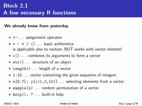
We already know from yesterday
• <- . . . assignment operator• + - * / () . . . basic arithmeticsis applicable also to vectors, BUT works with vector elemets!
• c() . . . combines its arguments to form a vector• str() . . . structure of an object• length() . . . length of a vector• 1:15 . . . vector containing the given sequence of integers• x[5:7]; y[c(1,2,10)] . . . selecting elements from a vector• sample(x) . . . random permutation of a vector• help(), ? . . . built-in help
ESSLLI ’2013 Hladká & Holub Day 2, page 3/78
Working with external files
• getwd() . . . to print the working directory• setwd() . . . to set your working directory• list.files() . . . to list existing files in your working directory
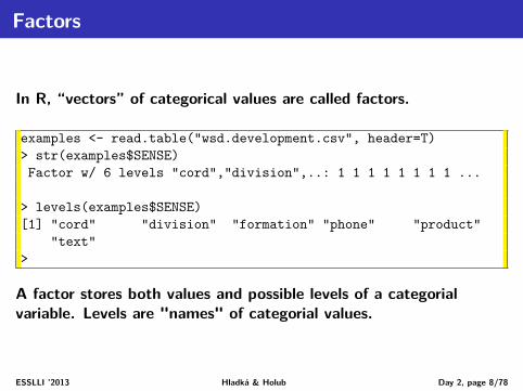
• read.table() . . . to load data from a .csv file– This function is the principal means of reading tabular data into R.
ESSLLI ’2013 Hladká & Holub Day 2, page 4/78
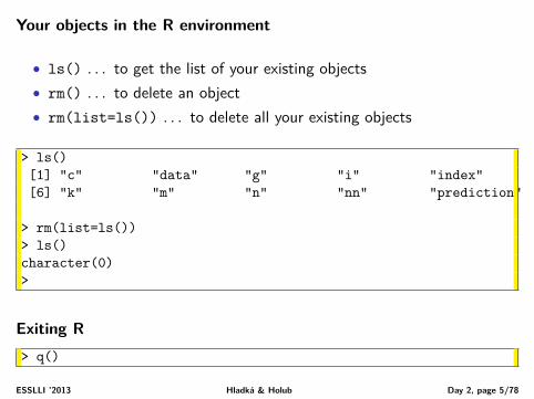
Your objects in the R environment
• ls() . . . to get the list of your existing objects• rm() . . . to delete an object• rm(list=ls()) . . . to delete all your existing objects
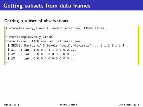
– Will retrieve first 20 observations and select only the 3 given variables.
ESSLLI ’2013 Hladká & Holub Day 2, page 13/78
Block 2.2Mathematics for machine learning
Machine learning requires some mathematical knowledge, especially
• statistics• probability theory• information theory• algebra (vector spaces)
ESSLLI ’2013 Hladká & Holub Day 2, page 14/78
Why statistics and probability theory?
Motivation
• In machine learning, models come from data and provide insights forunderstanding data or making prediction.
• A good model is often a model which not only fits the data but givesgood predictions, even if it is not interpretable.
Statistics
• is the science of the collection, organization, and interpretation ofdata
• uses the probability theory
ESSLLI ’2013 Hladká & Holub Day 2, page 15/78
Two purposes of statistical analysis
Statistics is the study of the collection, organization, analysis, andinterpretation of data. It deals with all aspects of this, including theplanning of data collection in terms of the design of surveys andexperiments.
Description
• describing what was observed in sample data numerically orgraphically
Inference
• drawing inferences about the population represented by thesample data
ESSLLI ’2013 Hladká & Holub Day 2, page 16/78
Random variables
A random variable (or sometimes stochastic variable) is, roughlyspeaking, a variable whose value results from a measurement/observationon some type of random process. Intuitively, a random variable is anumerical or categorical description of the outcome of a randomexperiment (or a random event).
Random variables can be classified as either
• discrete= a random variable that may assume either a finite number of valuesor an infinite sequence of values (countably infinite)
• continuous= a variable that may assume any numerical value in an interval orcollection of intervals.
ESSLLI ’2013 Hladká & Holub Day 2, page 17/78
Features as random variables
In machine learning theory we take features as random variables.
Target class is a random variable as well.
Data instance is considered as a vector of random values.
ESSLLI ’2013 Hladká & Holub Day 2, page 18/78
Probability theory – basic terms
Formal definitions• random experiment• elementary outcomes ωi
• sample space Ω =⋃ωi
• event A ⊆ Ω
• complement of an event Ac = Ω \ A• probability of any event is a non-negative value P(A) ≥ 0• total probability of all elementary outcomes is one∑
ω∈Ω
P(ω) = 1
• if two events A, B are mutually exclusive (i.e. A ∩ B = ∅), thenP(A ∪ B) = P(A) + P(B)
ESSLLI ’2013 Hladká & Holub Day 2, page 19/78
Basic formulas to calculate probabilities
Generally, probability of an event A is
P(A) =∑
ω∈AP(ω)
Probability of a complement event is
P(Ac) = 1− P(A)
ESSLLI ’2013 Hladká & Holub Day 2, page 20/78
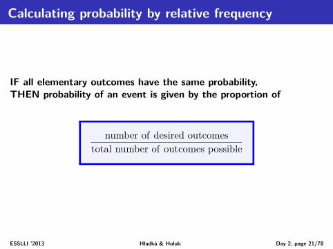
Calculating probability by relative frequency
IF all elementary outcomes have the same probability,THEN probability of an event is given by the proportion of
number of desired outcomestotal number of outcomes possible
ESSLLI ’2013 Hladká & Holub Day 2, page 21/78
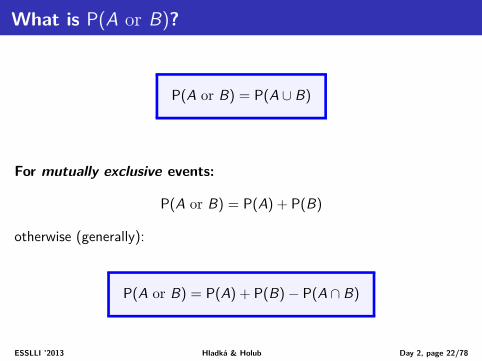
What is P(A or B)?
P(A or B) = P(A ∪ B)
For mutually exclusive events:
P(A or B) = P(A) + P(B)
otherwise (generally):
P(A or B) = P(A) + P(B)− P(A ∩ B)
ESSLLI ’2013 Hladká & Holub Day 2, page 22/78
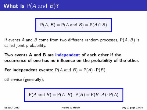
What is P(A and B)?
P(A, B) = P(A and B) = P(A ∩ B)
If events A and B come from two different random processes, P(A, B) iscalled joint probability.
Two events A and B are independent of each other if theoccurrence of one has no influence on the probability of the other.
For independent events: P(A and B) = P(A) · P(B).
otherwise (generally):
P(A and B) = P(A |B) · P(B) = P(B |A) · P(A)
ESSLLI ’2013 Hladká & Holub Day 2, page 23/78
Warming exercisesIf you want to make sure that you understand well basic probability computing
Rolling two dice, observing the sum. What is likelier?
a) the sum is evenb) the sum is greater than 8c) the sum is 5 or 7
What is likelier:
a) rolling at least one six in four throws of a single die, ORb) rolling at least one double six in 24 throws of a pair of dice?
ESSLLI ’2013 Hladká & Holub Day 2, page 24/78
Definition of conditional probability
Conditional probability of the event A given the event B is
P(A |B) =P(A ∩ B)
P(B)=
P(A, B)
P(B)
Or, in other words,
P(A, B) = P(A |B)P(B)
ESSLLI ’2013 Hladká & Holub Day 2, page 25/78
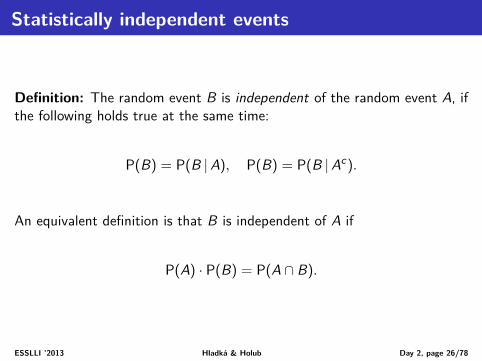
Statistically independent events
Definition: The random event B is independent of the random event A, ifthe following holds true at the same time:
P(B) = P(B |A), P(B) = P(B |Ac).
An equivalent definition is that B is independent of A if
P(A) · P(B) = P(A ∩ B).
ESSLLI ’2013 Hladká & Holub Day 2, page 26/78
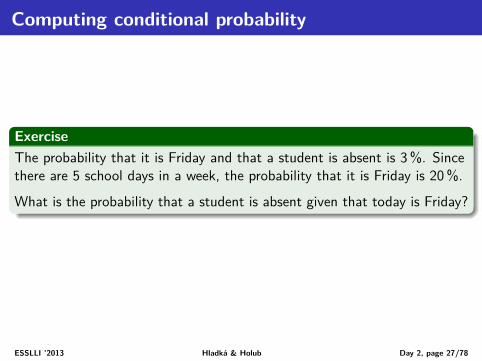
Computing conditional probability
ExerciseThe probability that it is Friday and that a student is absent is 3%. Sincethere are 5 school days in a week, the probability that it is Friday is 20%.
What is the probability that a student is absent given that today is Friday?
ESSLLI ’2013 Hladká & Holub Day 2, page 27/78
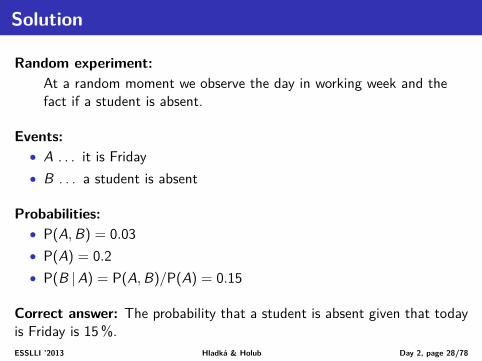
Solution
Random experiment:At a random moment we observe the day in working week and thefact if a student is absent.
Events:• A . . . it is Friday• B . . . a student is absent
Correct answer: The probability that a student is absent given that todayis Friday is 15%.ESSLLI ’2013 Hladká & Holub Day 2, page 28/78
Example – probability of target class
Look at the wsd.development data. There are 3524 examples in total.Each example can be considered as a random observation, i.e. as anoutcome of a random experiment.Occurrence of a particular value of the target class can be taken as an
event, similarly for other attributes.
Assume that• event A stands for SENSE = ‘PRODUCT’
• event B stands for A19 = ‘lines’
Then unconditioned probabilities Pr(A) and Pr(B) are
Pr(A) =number of observations with SENSE=‘PRODUCT’
number of all observations =18383524 = 52.16%
Pr(B) =number of observations with A19=‘lines’
number of all observations =11303524 = 32.07%
ESSLLI ’2013 Hladká & Holub Day 2, page 29/78
Example – conditional probability of target class
To compute conditional probability Pr(A |B) you need to know jointprobability Pr(A, B)
Pr(A, B) =number of observations with SENSE=‘PRODUCT’ and A19=‘lines’
number of all observations
Pr(A, B) =5193524 = 14.73%
Pr(A |B) =Pr(A, B)
Pr(B)=
14.73%
32.07%= 45.93%
Or, equivalently
Pr(A |B) =number of observations with SENSE=‘PRODUCT’ and A19=‘lines’
number of observations with A19=‘lines’
Pr(A |B) =5191130 = 45.93%
ESSLLI ’2013 Hladká & Holub Day 2, page 30/78
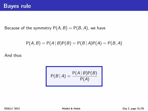
Bayes rule
Because of the symmetry P(A, B) = P(B, A), we have
P(A, B) = P(A |B)P(B) = P(B |A)P(A) = P(B, A)
And thus
P(B |A) =P(A |B)P(B)
P(A)
ESSLLI ’2013 Hladká & Holub Day 2, page 31/78
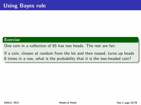
Using Bayes rule
ExerciseOne coin in a collection of 65 has two heads. The rest are fair.
If a coin, chosen at random from the lot and then tossed, turns up heads6 times in a row, what is the probability that it is the two-headed coin?
ESSLLI ’2013 Hladká & Holub Day 2, page 32/78
Solution
Random experiment and considered eventsWe observe if a chosen coin is two-headed (event A), and if all 6 randomtosses result in heads (event B). So, we want to know P(A |B).
Probabilities• P(A |B) is the probability that we are looking for
= P(B |A)P(A)/P(B) (application of Bayes rule)• P(B |A) = 1 (two-headed coin cannot give any other result)• P(A) = 1/65; P(Ac) = 64/65• P(B) = P(B, A) + P(B, Ac) (two mutually exclusive events)
1 Practise using R!Go thoroughly through all examples in our presentation and try it onyour own– using your computer, your hands, and your brain :–)
2 Study the Homework 1.1 Solution.Understand it. Especially the conditional probability computing.
ESSLLI ’2013 Hladká & Holub Day 2, page 34/78
Block 2.3Decision tree learning – Theory
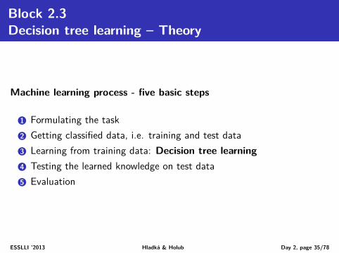
Machine learning process - five basic steps
1 Formulating the task2 Getting classified data, i.e. training and test data3 Learning from training data: Decision tree learning4 Testing the learned knowledge on test data5 Evaluation
ESSLLI ’2013 Hladká & Holub Day 2, page 35/78
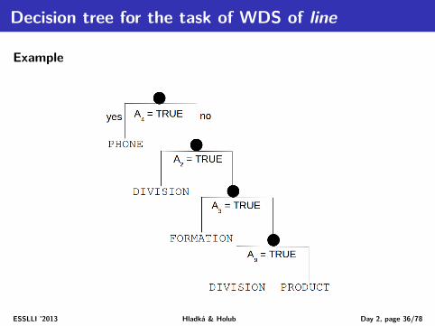
Decision tree for the task of WDS of line
Example
ESSLLI ’2013 Hladká & Holub Day 2, page 36/78
Using the decision tree for classification
Example
Assign the correct sense of line in the sentence "Draw a line between thepoints P and Q."
First, get twenty feature values from the sentence
A1 A2 A3 A4 A5 A6 A7 A8 A9 A10 A11
0 0 0 0 0 0 0 0 1 0 0
A12 A13 A14 A15 A16 A17 A18 A19 A20
a draw X between DT IN DT line dobj
ESSLLI ’2013 Hladká & Holub Day 2, page 37/78
Using the decision tree for classification
Second, get the classification of the instance using the decision tree
ESSLLI ’2013 Hladká & Holub Day 2, page 38/78
Using the decision tree for classification
Example
Assign the correct sense of line in the sentence "Draw a line that passesthrough the points P and Q."
First, get twenty feature values from the sentence
A1 A2 A3 A4 A5 A6 A7 A8 A9 A10 A11
0 0 0 0 0 0 0 0 0 0 0
A12 A13 A14 A15 A16 A17 A18 A19 A20
a draw X that DT WDT VB line dobj
ESSLLI ’2013 Hladká & Holub Day 2, page 39/78
Using the decision tree for classification
Second, get the classification of the instance using the decision tree
ESSLLI ’2013 Hladká & Holub Day 2, page 40/78
Building a decision tree from training data
Tree structure description
• Nodes• Root node• Internal nodes• Leaf nodes with TARGET
CLASS VALUES• Decisions
• Binary questions on a singlefeature, i.e. each internalnode has two child nodes
ESSLLI ’2013 Hladká & Holub Day 2, page 41/78
Building a decision tree from training data
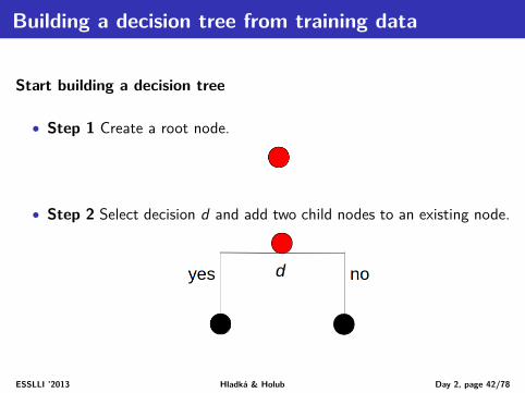
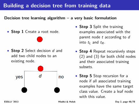
Start building a decision tree
• Step 1 Create a root node.
• Step 2 Select decision d and add two child nodes to an existing node.
ESSLLI ’2013 Hladká & Holub Day 2, page 42/78
Building a decision tree from training data
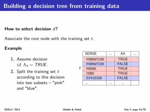
How to select decision d?
Associate the root node with the training set t.
Example
1. Assume decisionif A4 = TRUE .
2. Split the training set taccording to this decisioninto two subsets – "pink"and "blue".
t
SENSE ... A4 ...FORMATION TRUEFORMATION FALSEPHONE TRUECORD TRUEDIVISION FALSE
... ... ...
ESSLLI ’2013 Hladká & Holub Day 2, page 43/78
Building a decision tree from training data
3. Add two child nodes, "pink" and"blue", to the root. Associateeach of them with thecorresponding subset tL, tR ,resp.
tL
SENSE ... A4 ...FORMATION TRUECORD TRUEPHONE TRUE
... ... ...
tR
SENSE ... A4 ...FORMATION FALSEDIVISION FALSE
... ... ...
ESSLLI ’2013 Hladká & Holub Day 2, page 44/78
Building a decision tree from training data
How to select decision d?
Working with more than one feature, more than one decision can beformulated.
Which decision is the best?
Focus on a distribution of target class values in associated subsets oftraining examples.
ESSLLI ’2013 Hladká & Holub Day 2, page 45/78
Building a decision tree from training data
Example
• Assume a set of 120 training examples from the task of WSD.• Some decision splits them into two sets (1) and (2) with the followingtarget class value distribution:
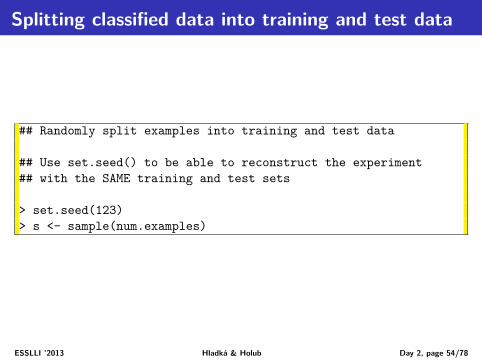
Splitting classified data into training and test dataSecond, split them into the training and test sets
## Get the number of input examples> num.examples <- nrow(examples)
## Set the number of training examples = 90% of examples> num.train <- round(0.9 * num.examples)
## Set the number of test examples = 10% of examples> num.test <- num.examples - num.train
## Check the numbers> num.examples[1] 3524> num.train[1] 3172> num.test[1] 352
ESSLLI ’2013 Hladká & Holub Day 2, page 52/78
Splitting classified data into training and test data
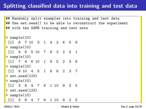
## Randomly split examples into training and test data## Use set.seed() to be able to reconstruct the experiment## with the SAME training and test sets
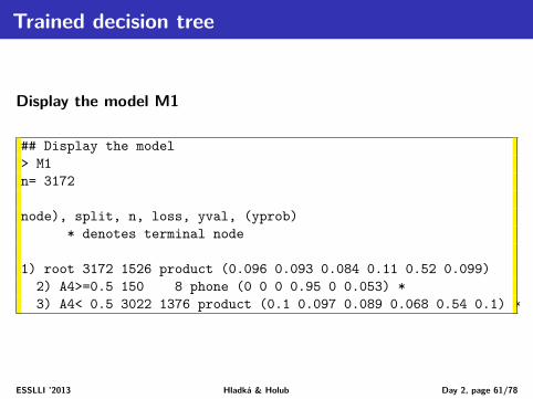
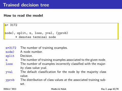
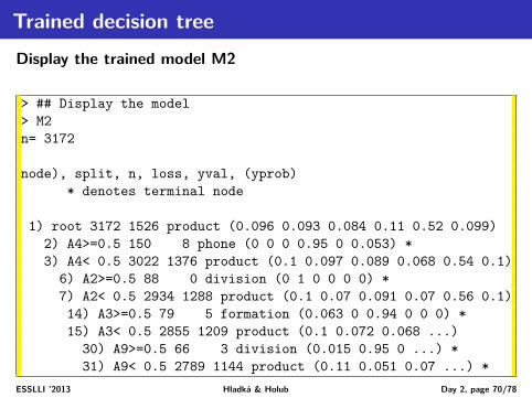
node), split, n, loss, yval, (yprob)* denotes terminal node
n=3172 The number of training examples.node) A node number.split Decision.n The number of training examples associated to the given node.loss The number of examples incorrectly classified with the major-
ity class value yval.yval The default classification for the node by the majority class
value.yprob The distribution of class values at the associated training sub-
set.ESSLLI ’2013 Hladká & Holub Day 2, page 62/78
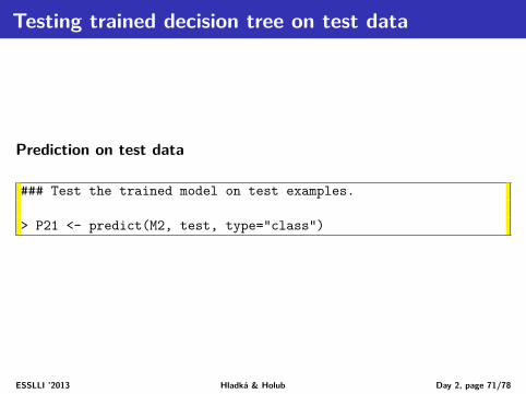
Testing trained decision tree on test data
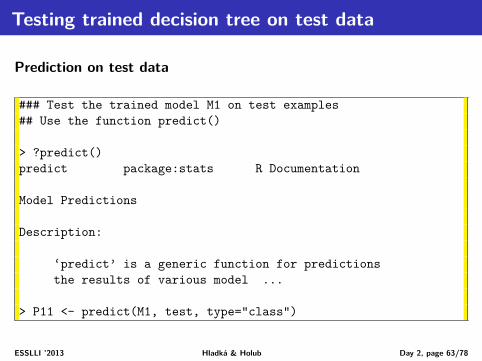
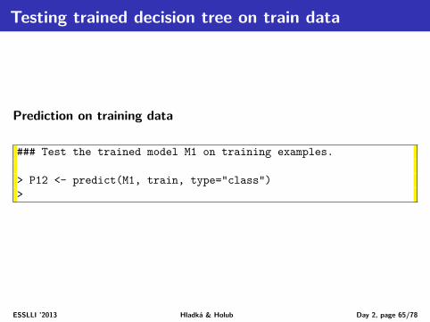
Prediction on test data
### Test the trained model M1 on test examples## Use the function predict()
> ?predict()predict package:stats R Documentation
Model Predictions
Description:
‘predict’ is a generic function for predictionsthe results of various model ...
> P11 <- predict(M1, test, type="class")
ESSLLI ’2013 Hladká & Holub Day 2, page 63/78
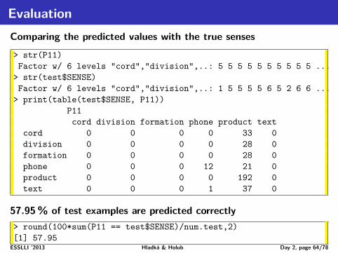
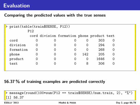
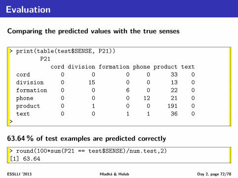
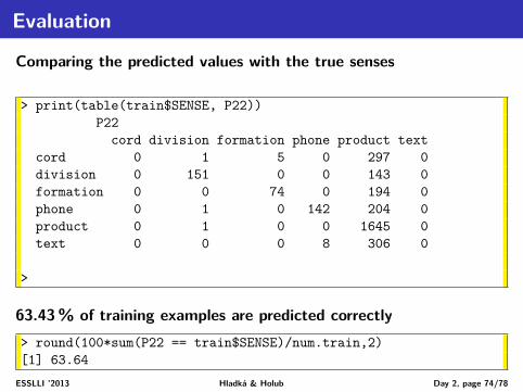
EvaluationComparing the predicted values with the true senses
63.43% of training examples are predicted correctly> round(100*sum(P22 == train$SENSE)/num.train,2)[1] 63.64
ESSLLI ’2013 Hladká & Holub Day 2, page 74/78
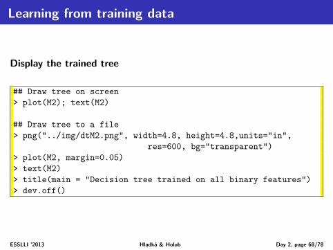
Run the script in R
The R script DT-WSD.R
• builds the classifier M1 using the feature A4, classifies training andtest data using M1 and computes the performance of M1.
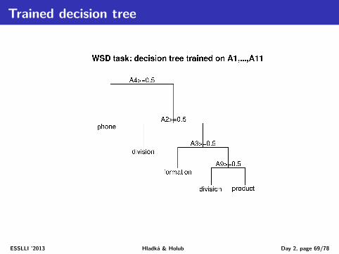
• builds the classifier M2 using binary features A1, ..., A11, classifiestraining and test data using M2 and computes the performance of M2.
Download the script from the course page and run in R
> source("DT-WSD.R")>
ESSLLI ’2013 Hladká & Holub Day 2, page 75/78
Homework 2.2
Generate the same training and test sets as we did in practice above.Assume the following feature groups:
1 A2, A3, A4, A9
2 A1, A6, A7
3 A1, A11
For each of them, build a decision tree classifier and list its percentage ofcorrectly classified training and test examples.
ESSLLI ’2013 Hladká & Holub Day 2, page 76/78
Summary of Day 2
Theory
• Decision tree structure: nodes, decisions• A basic formulation of decision tree learning algorithm
ESSLLI ’2013 Hladká & Holub Day 2, page 77/78
Summary of Day 2
Practice
We built two decision tree classifiers (M1, M2) on two different sets offeatures and we tested them on both training and test sets.
features used trained model data set performanceA4 M1
train 57.37test 57.95
A1, ..., A11 M2train 63.43test 63.64
!!! You know how to build a decision tree classifier from trainingexamples in R. Performance is not important right now. !!!ESSLLI ’2013 Hladká & Holub Day 2, page 78/78