AGGREGATE EXPENDITURES

Frederick University 2014

Aggregate Demand (AD)

AD – the quantity of GDP, which the economic agents are planning to buy at every price level, ceteris paribus (Y = const)

Aggregate Expenditures

АЕ – the expenditures that economic decision makers are planning to make at every level of income, ceteris paribus

Planned Spending Real GDP = Nominal GDP AE = C + I + G + X - M

Consumption Spending (С)

С – the expenditures that households are planning to make at every level of income, ceteris paribus

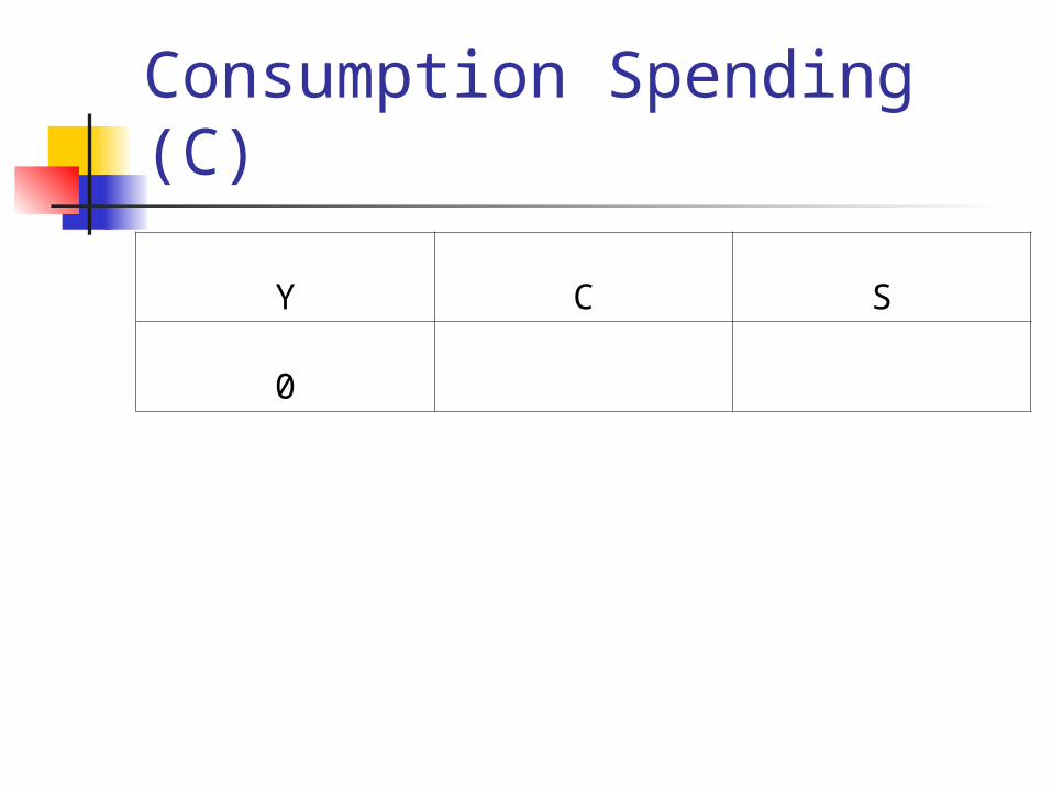
Consumption Spending (С)

Y C S

0

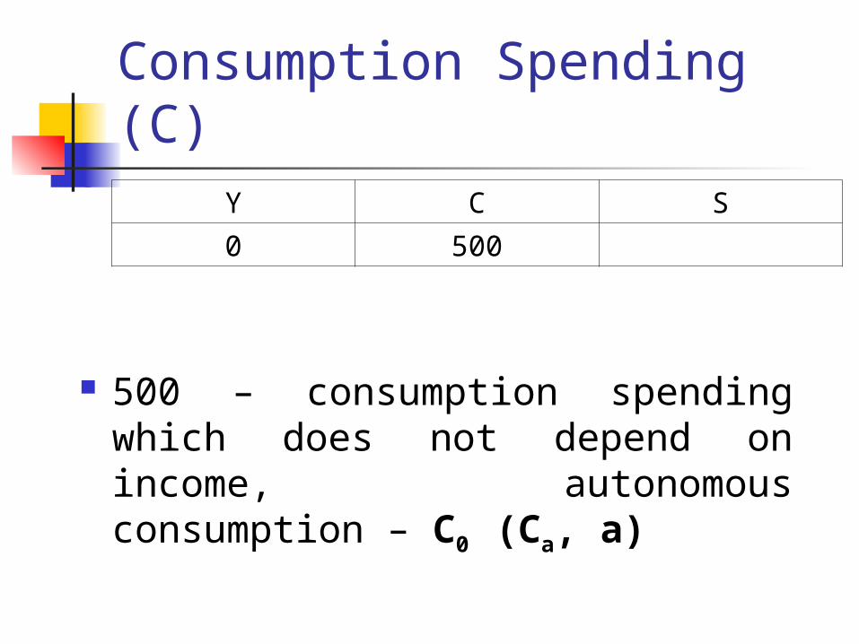
Consumption Spending (С) Y C S

0 500

500 – consumption spending which does not depend on income, autonomous consumption – С0 (Ca, a)

Consumption Spending (С)

Y C S

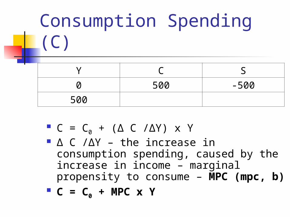
0 500 -500

Consumption Spending (С)

Y C S

0 500 -500

500

C = C0 + (Δ C /ΔY) x Y Δ C /ΔY – the increase in consumption

spending, caused by the increase in income – marginal propensity to consume – MPC (mpc, b)

C = C0 + MPC x Y

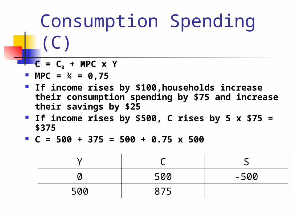
Consumption Spending (С) C = C0 + MPC x Y MPC = ¾ = 0,75 If income rises by $100,households increase their

consumption spending by $75 and increase their savings by $25

If income rises by $500, С rises by 5 х $75 = $375 C = 500 + 375 = 500 + 0.75 x 500

Y C S

0 500 -500

500 875

Savings (S) Marginal propensity to save – the increase in

savings, caused by the increase in income: MPS = Δ S /ΔY If income rises by $100, and households raise

their consumption spending by $75, savings increase by $25

MPC + MPS = 1 C + S = Y S = Y – C = Y – (C0 + MPC x Y) = Y - C0 - MPC x

Y = - C0 + Y - MPC x Y = - C0 + Y(1 - MPC) S = - C0 + MPS x Y

Consumption Spending (С) and Savings (S)

Y C S

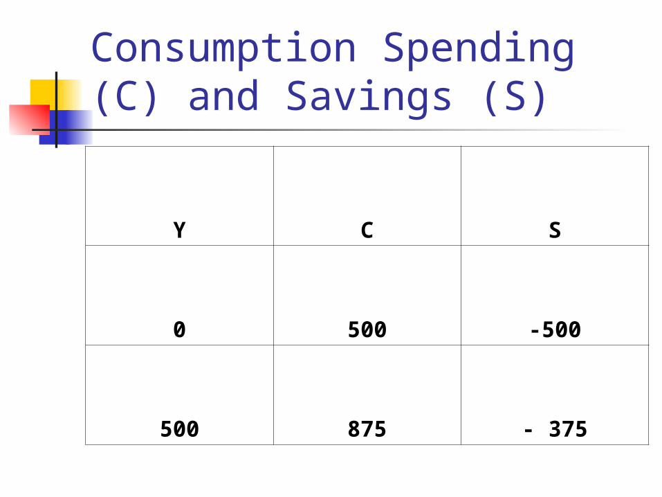
0 500 -500

500 875 - 375

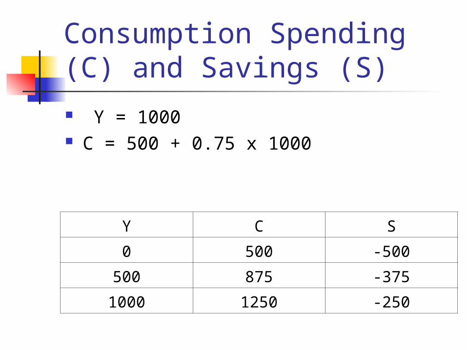
Consumption Spending (С) and Savings (S) Y = 1000 C = 500 + 0.75 x 1000

Y C S

0 500 -500

500 875 -375

1000 1250 -250

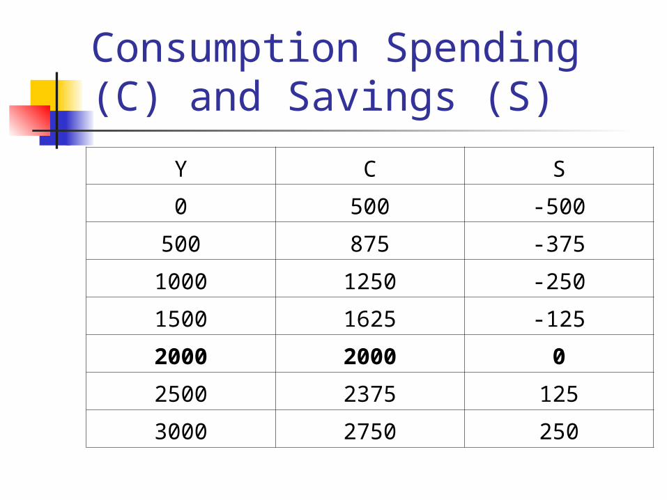
Consumption Spending (С) and Savings (S)

Y C S

0 500 -500

500 875 -375

1000 1250 -250

1500 1625 -125

2000 2000 0

2500 2375 125

3000 2750 250

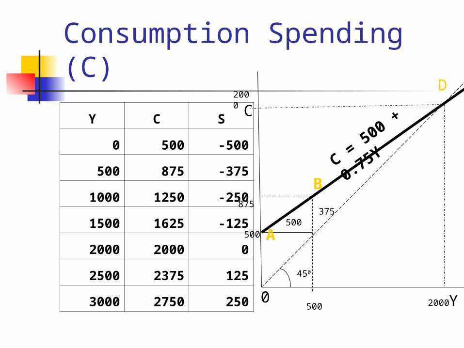
Consumption Spending (С)

Y C S

0 500 -500

500 875 -375

1000 1250 -250

1500 1625 -125

2000 2000 0

2500 2375 125

3000 2750 250

450

C

Y

500

2000

2000500

875

500375

C = 500 + 0.75Y

0

A

B

D

Factors determining C Households’ income Indirect taxation Propensity to buy imported goods and services Direct taxation Consumers’ expectations Availability of consumer credit Income distribution Living standards Efficiency of market institutions

Investment spendingI = Gross Private Domestic Investment I – Depreciation = Net Investment Net investment = Purchases of New

Equipment + Change in Inventories Fixed Investment = Depreciation + Purchases

of New Equipment Net Fixed Investment = Purchases of New

Equipment Inventories = Raw Material + Unfinished Production + Finished Goods

Factors determining Investment Spending (I)

Interest rate (i) Expected future profits (π) Risk Excess capacity Capital-output ratio (α) Technological changes Cost of production Competitiveness of markets Depreciation policies Efficiency of market institutions

AE

450

C

Y

500

2000

2000500

875

500375

0

A

B

D

CAE = C

+ I +

G +

X -

M

AE

0

5001000

1500

2000

25003000

3500

0 1000 2000 3000 4000

Y

AE

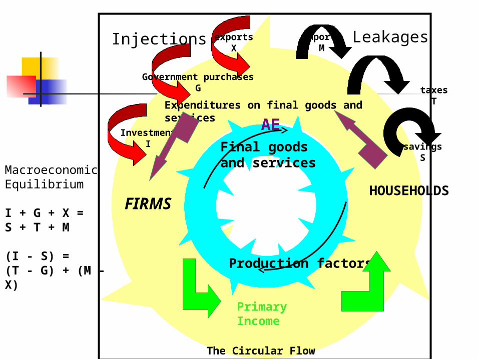
HOUSEHOLDSFIRMS

Expenditures on final goods and services

Primary Income

importsМ

taxesТ

savingsS

exportsХ

Government purchasesG

InvestmentІ

LeakagesInjections

Production factors

Final goods and services

The Circular Flow

AE

Macroeconomic Equilibrium

I + G + X =S + T + M

(I - S) = (T - G) + (M - X)

Macroeconomic Equilibrium

Y < AE Reduction of inventories Y Y = AE Y > AE Increase in inventories Y Y = AE

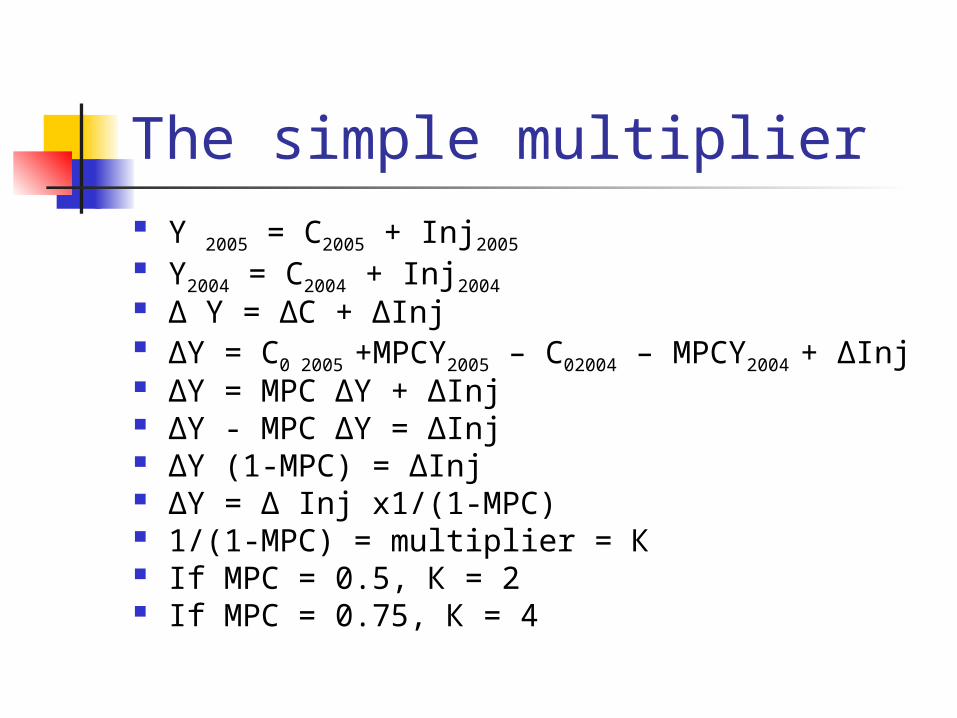
The simple multiplier Y 2005 = C2005 + Inj2005 Y2004 = C2004 + Inj2004 Δ Y = ΔC + ΔInj ΔY = C0 2005 +MPCY2005 – C02004 – MPCY2004 + ΔInj ΔY = MPC ΔY + ΔInj ΔY - MPC ΔY = ΔInj ΔY (1-MPC) = ΔInj ΔY = Δ Inj x1/(1-MPC) 1/(1-MPC) = multiplier = К If МРС = 0.5, К = 2 If МРС = 0.75, К = 4

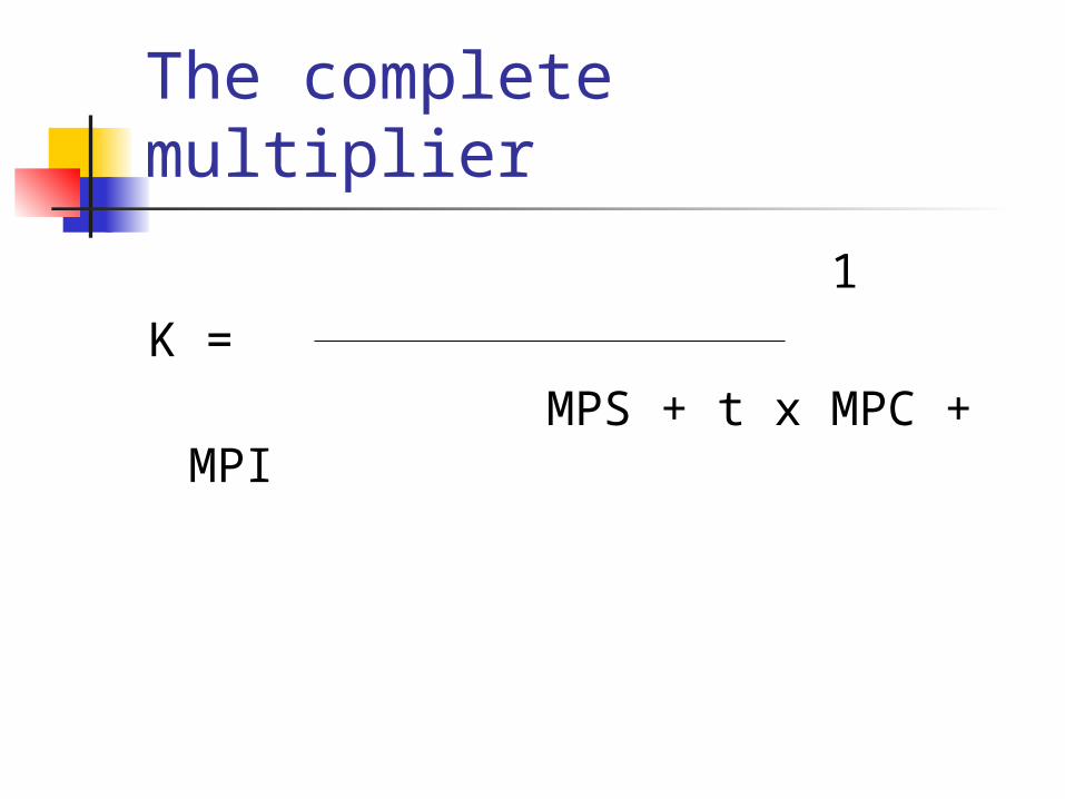
The complete multiplier

1K = MPS + t x MPC + MPI

Multiplier Constraints

Factors of production bottlenecks Limited productive capacity Institutions

Deriving the Complete Multiplier Y 2005 = C2005 + (I + G + X)2005 - M2005 Y2004 = C2004 + (I + G + X)2004 - M2004 Δ Y = ΔC + ΔInj - ΔM ΔY = C0 2005 +MPC x (Y2005 – t x Y2005) - C02004 – MPC x (Y2004 – t x

Y2004) + ΔInj - M0 2005 – MPI x (Y2005 – t x Y2005) - M02004 – MPI x (Y2004 – t x Y2004) + ΔInj

ΔY = MPC x Y2005 ( 1– t x) – MPC x Y2004 ( 1 - t) - MPI x Y2005 ( 1– t) – MPI x Y2004 (1– t)

ΔY = MPC ( 1 - t) x ΔY – MPI x ΔY + ΔInj ΔY - MPC ( 1 - t) ΔY + MPI x ΔY = ΔInj ΔY [(1-MPC + MPC x t) + MPI] = ΔInj ΔY = Δ Inj :1/(1-MPC + MPC x t + MPI) K = 1/(1-MPC + MPC x t + MPI) = 1/ (MPS + MPT + MPI)