Aggregate interlock - TU Delft

Faculty of Civil Engineering and Geosciences Department of Structural and Building Engineering

; 12

Aggregate Interlock Extending the aggregate interlock model to high strength concrete

Stamatia Presvyri

| ii

Aggregate Interlock Extending the aggregate interlock model to high strength

concrete

By

Stamatia Presvyri

in partial fulfilment of the requirements for the degree of

Master of Science

in Civil Engineering

at the Delft University of Technology,

to be defended publicly on Tuesday January 22, 2019 at 15:30.

Supervisor: Dr. ir. Y. Yang, TU Delft

Thesis committee: Dr. J.H.M. Visser, TNO

Dr. ir M.A.N. Hendriks, TU Delft

Prof. dr. ir. D.A. Hordijk, TU Delft

Study Program Coordinator: Ir. L.J.M. Houben, TU Delft

An electronic version of this thesis is available at http://repository.tudelft.nl/.

http://repository.tudelft.nl/

| iii

Cover illustration: Shear failure of a beam

Copyright © 2019 by Stamatia Presvyri

| iv

Preface This master thesis is submitted as a partial fulfilment of the requirements for the Master of Science degree in Structural Engineering, with a specialization in Concrete Structures at the Delft University of Technology. This work could not have been possible without the support of many people.

First of all, I would like to express my gratitude to my supervisor, Yuguang Yang, for his continuous support, guidance and encouragement throughout this period. I am grateful for giving me the opportunity to work on this interesting topic and for sharing his deep knowledge, experience and enthusiasm regarding this. Furthermore, I would like to thank the members of my thesis committee Prof. dr. ir. Dick Hordijk, Dr. Jeanette Visser and Dr. ir. Max Hendriks for their valuable advices and interesting remarks.

I would like to acknowledge the Gemeente of Rotterdam, for borrowing the laser scanner station, which provided me with valuable results that contributed to the completion of my project.

Moreover, I would like to thank my friends for their continuous encouragement and the enjoyable time during this period. Special thanks to Dimitris for his useful advices about the coding part, that helped me to overcome some difficulties. Also, I am very grateful to my boyfriend, Marios, who was always by my side, supporting and giving me valuable help throughout the difficult times.

Finally, I would like to thank my family, Manolis, Lefki and Socrates, for their endless love, encouragement and support during my whole life. I couldn’t have done this without them.

Stamatia Presvyri

Delft, January 2019

| v

| vi

Abstract The shear capacity of concrete members is a major challenge of structural concrete research through the years. Many theoretical models have been developed and various experiments have been performed, focusing on the accurate prediction of the shear behavior. Many of the available theoretical models assume that a large contribution of the shear capacity is transferred through cracks by a mechanism often recognized as aggregate interlock. At the same time, due to the increase in the complexity of the structures and the development of the concrete technology, the mechanical properties of concrete have improved significantly. This fact leads to the need for modification of the existing models or the development of new ones, accommodated to the improved materials.

Since, the aggregate interlock plays a significant role in the development of the shear capacity, the present research proposes a new numerical methodology for the calculation of the aggregate interlock in high strength concrete in which aggregates break, based on the widely recognized model proposed by Walraven and the results of direct surface roughness measurements.

The crack surfaces of concrete cylindrical specimens drilled from a 70 years old existing concrete bridge and newly casted cubic specimens generated by splitting tensile tests were measured by a laser scanner. Moreover, the surface of a reinforced deep beam after flexural shear failure was measured as well. The measured crack surfaces were used to implement the plasticity based aggregate interlock model proposed by Walraven with an algorithm which was validated with Walraven’s theoretical model, using a so-called mesostructural model. The output of the analysis gave suggestions on the adjustment of the available aggregate interlock model for high strength concrete.

The proposed model is then implemented into a shear test on a 1.2 m concrete beam, which has a concrete strength larger than 70 MPa and the aggregate interlock seems to influence significantly the shear resistance of a cracked section.

Based on the observation of the surface roughness of a crack, the thesis further proposed that with a sufficiently large crack face, the localized variation in the crack surface is averaged out. Thus, the surface can be used to develop a master curve for the given concrete type.

In the last part of the study, two improvement suggestions are given regarding the Critical Shear Displacement Theory. The one point is relevant to the simplification of the crack profile that can be changed from a straight line into a more inclined and the second point is related to the correction factor considering the fracture of the aggregates, that should be dependent on the crack width.

| vii

| viii

Notation Abbreviations

AASHTO American Association of State Highway and Transportation Officials ACI American Concrete Institute CDM Contact Density Model CSA Canadian Standards Association CSDT Critical Shear Displacement Theory DIC Digital Image Correlation EC2 Eurocode 2 fib International Federation for Structural Concrete LVDT Linear Variable Differential Transformer, a sensor used to measure

deformations in a single direction

Roman upper case

𝐴𝐴𝑐𝑐 concrete area 𝐴𝐴𝑐𝑐v area of concrete shear interface 𝛢𝛢𝑡𝑡 total area of crack surface 𝐴𝐴𝑣𝑣f area of interface shear reinforcement 𝐴𝐴𝑥𝑥 projection of total contact area on x-plane 𝐴𝐴𝑦𝑦 projection of total contact area on y-plane 𝐶𝐶𝐶𝐶 fracture index 𝐶𝐶𝑅𝑅d,𝑐𝑐 coefficient derived from tests (EC2) 𝐷𝐷𝑚𝑚𝑚𝑚𝑥𝑥 maximum aggregate size 𝐷𝐷𝑚𝑚𝑚𝑚𝑚𝑚 minimum aggregate size 𝐸𝐸𝑠𝑠 Young’s modulus of steel 𝐾𝐾(𝑤𝑤) ratio of effective contact area 𝑃𝑃c permanent net compressive strength 𝑅𝑅𝑚𝑚𝑚𝑚 reduction factor of aggregate interlock 𝑅𝑅𝑐𝑐 contact normal force 𝑉𝑉𝑚𝑚𝑚𝑚 shear force component carried by aggregate interlock 𝑉𝑉𝑐𝑐 shear force component carried in the uncracked concrete compression zone 𝑉𝑉𝑑𝑑 shear force component carried by dowel action 𝑉𝑉𝑅𝑅,𝑑𝑑𝑐𝑐 design value of the shear capacity

https://en.wikipedia.org/wiki/List_of_welding_codes#Canadian_Standards_Association_(CSA)_Standards

| ix

Roman lower case

𝑏𝑏𝑤𝑤 web width 𝑐𝑐 cohesion factor 𝑑𝑑 effective height of cross section 𝑑𝑑𝑚𝑚ax/𝑑𝑑min the maximum/minimum sizes of aggregate particles within a grading segment 𝐶𝐶′𝑐𝑐𝑐𝑐 crushing strength of cement matrix 𝐶𝐶𝑐𝑐𝑐𝑐 characteristic concrete cylinder compressive strength 𝐶𝐶𝑐𝑐𝑚𝑚 mean concrete compressive strength (through standard cylinder tests) fc,cube mean concrete compressive strength (through standard cube tests) 𝐶𝐶𝑦𝑦 yield strength of steel 𝐶𝐶y,𝑐𝑐r tensile stress in longitudinal reinforcement at the crack surface 𝑘𝑘 size effect factor 𝑛𝑛 tension-to-shear loading ratio 𝑝𝑝𝑘𝑘 the aggregate area fraction w crack width

Greek upper case

Δ shear displacement 𝛺𝛺(𝜃𝜃) contact density function

Greek lower case

𝑎𝑎 coefficient for interface / pre-crack condition 𝛽𝛽 factor for tensile stresses (SMCFT) 𝛾𝛾𝑐𝑐 partial safety factor of the concrete according to the design situation 𝜃𝜃 angle of contact stress 𝜇𝜇 coefficient of friction 𝜌𝜌𝑠𝑠 reinforcement ratio σ normal stress at the crack surface 𝜎𝜎𝑐𝑐on(𝜃𝜃) contact stress 𝜎𝜎𝑝𝑝u matrix yielding strength τ shear stress at the crack surface τmax maximum shear stress that can be resisted by aggregate interlock 𝜑𝜑𝑐𝑐 shear capacity reduction factor (CSA code)

| x

Table of Contents

1 Introduction ...................................................................................................................... 1

1.1 Problem Definition .................................................................................................... 1

1.1.1 Shear failure ...................................................................................................... 1

1.1.2 Definition of aggregate interlock ........................................................................ 2

1.2 Aggregate interlock in current design codes ............................................................ 3

1.2.1 fib Model Code 2010 & Canadian code (CSA) .................................................. 3

1.2.2 EC2 & ACI-318 .................................................................................................. 4

1.2.3 Conclusions ....................................................................................................... 4

1.3 Research Objectives ................................................................................................ 5

1.4 Research Methodology ............................................................................................. 5

1.4.1 Literature Review .............................................................................................. 5

1.4.2 Measurements of surface roughness ................................................................ 5

1.4.3 Numerical Approach .......................................................................................... 6

1.5 Thesis Outline ........................................................................................................... 7

2 Literature Review ............................................................................................................. 9

2.1 Theoretical Models ................................................................................................... 9

2.1.1 Empirical models ............................................................................................... 9

2.1.2 Physical models .............................................................................................. 11

2.1.3 Conclusions ..................................................................................................... 21

2.2 Experimental Research .......................................................................................... 21

2.2.1 Conclusions ..................................................................................................... 24

3 Numerical simulation of Walraven’s model .................................................................... 25

3.1 Definition of the numerical mesoscale modelling ................................................... 25

3.2 Numerical simulation .............................................................................................. 26

3.2.1 Assumptions .................................................................................................... 26

3.2.2 Description of the procedure ........................................................................... 26

3.3 Validation of the model ........................................................................................... 30

3.3.1 Case 1 ............................................................................................................. 31

3.3.2 Case 2 ............................................................................................................. 32

3.4 Conclusions ............................................................................................................ 33

4 Surface roughness measurements ................................................................................ 35

| xi

4.1 Test Program .......................................................................................................... 35

4.1.1 Specimens ....................................................................................................... 35

4.2 Roughness Measurements ..................................................................................... 37

5 Crack Surface Geometry ............................................................................................... 39

5.1 Post-processing of laser scanning data .................................................................. 39

5.2 Surface Roughness Index ...................................................................................... 40

5.3 Angle distribution .................................................................................................... 43

5.4 Conclusions ............................................................................................................ 47

6 Aggregate interlock based on measured crack surfaces ............................................... 49

6.1 Adoption of the numerical approach to scanned surfaces ...................................... 49

6.2 Fracture of the aggregates ..................................................................................... 50

6.3 Beam Study ............................................................................................................ 55

6.3.1 I603A Results .................................................................................................. 57

6.3.2 Influence of the segments’ length in crack profile ........................................... 58

6.3.3 Master curve .................................................................................................... 61

6.4 Conclusions ............................................................................................................ 63

7 Conclusions & Recommendations ................................................................................. 65

7.1 Conclusions ............................................................................................................ 65

7.2 Recommendations .................................................................................................. 66

Bibliography .......................................................................................................................... 67

Table of figures ..................................................................................................................... 71

Appendix A ............................................................................................................................ 73

Appendix B ............................................................................................................................ 83

| 1

Fig. 1.2: Shear compression failure Fig. 1.1: Flexural shear failure

1 Introduction

1.1 Problem Definition In structural design, the determination of shear capacity is a very complicated process and the shear failure causes many disasters, or even collapses. During the years, many models have been developed trying to accurately describe the shear behavior and the shear transfer mechanisms that affect it. Although, there is not yet a model that predicts precisely the shear capacity. In particular, the old concrete structures used low strength concrete and aggregates with very large size. So, the crack faces of this “old concrete” are complicated and the prediction of the failure is difficult. These facts arise safety issues for the existing structures and the construction of new structures.

On the other hand, nowadays the growth of the population, the construction of big and complex projects, the development of the technology and the environmental pollution lead to the development of new strong, durable and sustainable materials. Because of that, the demand for high strength concrete and concrete with lightweight or recycled aggregates increases constantly and leads to the change to the composition of concrete throughout the years. In the past, the strength of the concrete was lower, and the aggregate sizes, strengths and types were different. Therefore, the existing models about shear failure describe the behavior of this “old concrete”.

Due to the reasons mentioned above, a general model about the shear behavior that will include the older and the current composition and properties of concrete is necessary.

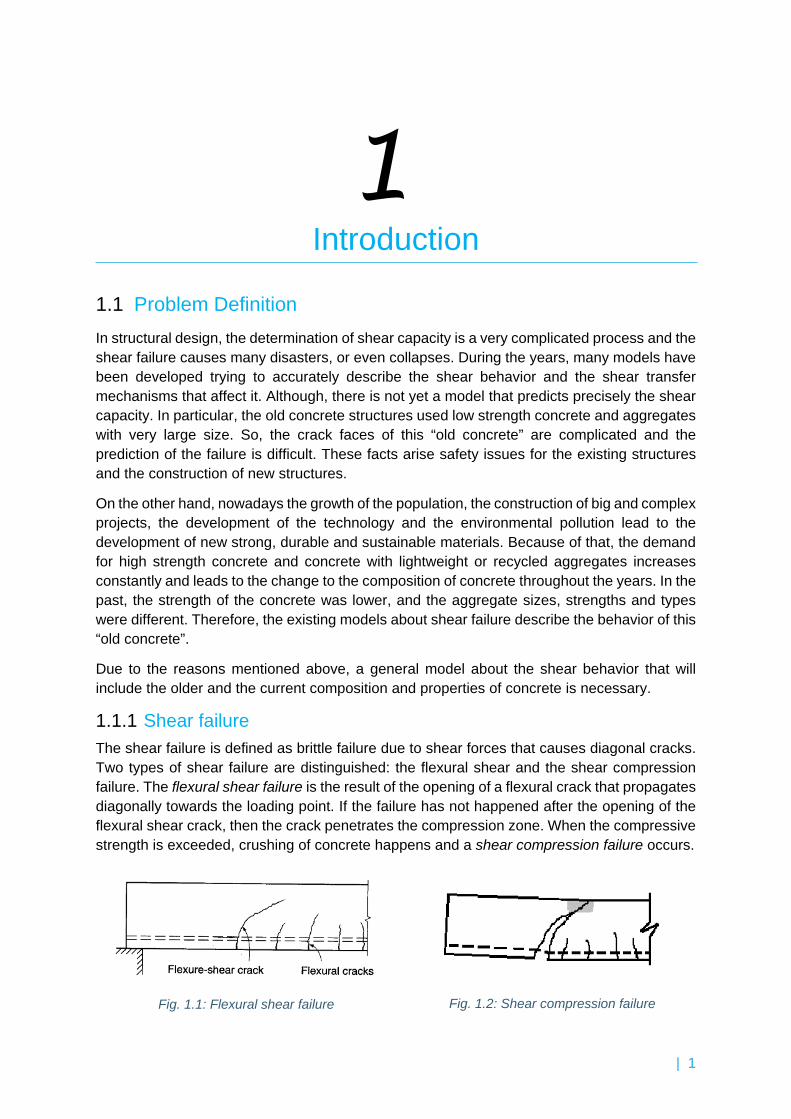
1.1.1 Shear failure The shear failure is defined as brittle failure due to shear forces that causes diagonal cracks. Two types of shear failure are distinguished: the flexural shear and the shear compression failure. The flexural shear failure is the result of the opening of a flexural crack that propagates diagonally towards the loading point. If the failure has not happened after the opening of the flexural shear crack, then the crack penetrates the compression zone. When the compressive strength is exceeded, crushing of concrete happens and a shear compression failure occurs.

1. Introduction

| 2

1.1.2 Definition of aggregate interlock As it is known, the cracks can transmit shear forces. In cracked concrete members without shear reinforcement, there are three principal transfer mechanisms [1]:

1) the direct shear transfer in the concrete compressive zone (Vc) 2) the dowel action (Vd) of the longitudinal reinforcement and 3) the aggregate interlock (Vai)

The aggregate interlock occurs when shear displacements act between two cracked surfaces. The protruding aggregate particles form contact areas on their surfaces, which produce stresses, during the relative slip and friction between the two faces. This mechanism is directly related to the roughness of the crack surfaces and the crack kinematics. Four main parameters that characterize the aggregate interlock mechanism are: the crack width, the shear displacement, the normal and the shear stresses.

In the normal strength concrete, the strength of the hardened cement paste is lower than the strength of the aggregate particles and the crack propagates around the aggregates. On the other hand, in high strength concrete the strength of cement matrix is higher and the crack propagates through the aggregates, resulting in smoother crack surfaces.

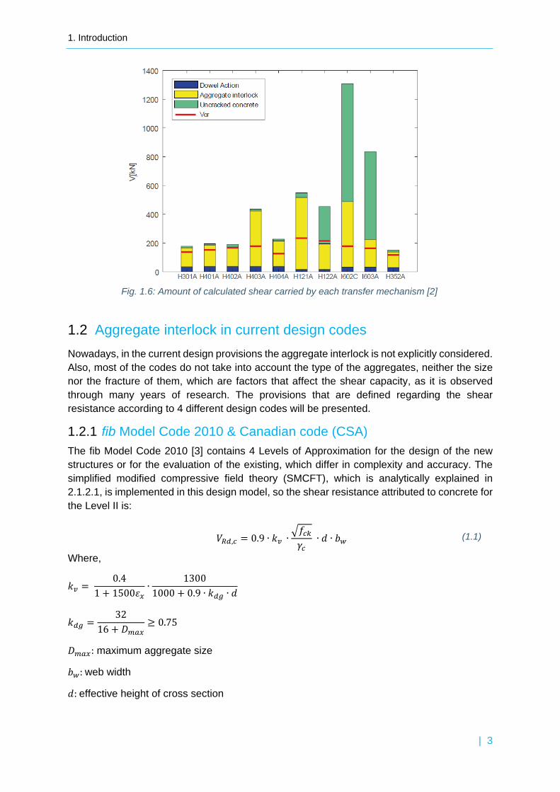
A recent research at TU Delft about the analysis of shear transfer mechanisms in concrete members [2] concluded that the aggregate interlock contributes significantly to the shear capacity. Especially, in flexural shear failure the aggregate interlock is the governing mechanism. The results of this research are depicted in Fig. 1.6. So, this was a motivation for the subject of this research, which focuses to the further study of aggregate interlock.

Fig. 1.3: Shear transfer mechanisms [1]

Fig. 1.5: Crack propagation in HSC [1] Fig. 1.4: Crack propagation in NSC [11]

1. Introduction

| 3

Fig. 1.6: Amount of calculated shear carried by each transfer mechanism [2]

1.2 Aggregate interlock in current design codes Nowadays, in the current design provisions the aggregate interlock is not explicitly considered. Also, most of the codes do not take into account the type of the aggregates, neither the size nor the fracture of them, which are factors that affect the shear capacity, as it is observed through many years of research. The provisions that are defined regarding the shear resistance according to 4 different design codes will be presented.

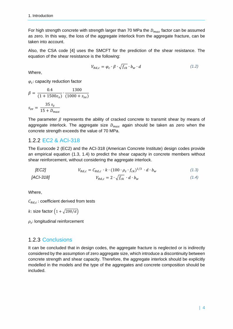
1.2.1 fib Model Code 2010 & Canadian code (CSA) The fib Model Code 2010 [3] contains 4 Levels of Approximation for the design of the new structures or for the evaluation of the existing, which differ in complexity and accuracy. The simplified modified compressive field theory (SMCFT), which is analytically explained in 2.1.2.1, is implemented in this design model, so the shear resistance attributed to concrete for the Level II is:

𝑉𝑉𝑅𝑅𝑑𝑑,𝑐𝑐 = 0.9 ∙ 𝑘𝑘𝑣𝑣 ∙�𝐶𝐶𝑐𝑐𝑐𝑐𝛾𝛾𝑐𝑐

∙ 𝑑𝑑 ∙ 𝑏𝑏𝑤𝑤 (1.1)

Where,

𝑘𝑘𝑣𝑣 = 0.4

1 + 1500𝜀𝜀𝑥𝑥∙

13001000 + 0.9 ∙ 𝑘𝑘𝑑𝑑𝑑𝑑 ∙ 𝑑𝑑

𝑘𝑘𝑑𝑑𝑑𝑑 =32

16 + 𝐷𝐷𝑚𝑚𝑚𝑚𝑥𝑥≥ 0.75

𝐷𝐷𝑚𝑚𝑚𝑚𝑥𝑥: maximum aggregate size

𝑏𝑏𝑤𝑤: web width

𝑑𝑑: effective height of cross section

1. Introduction

| 4

For high strength concrete with strength larger than 70 MPa the 𝐷𝐷𝑚𝑚𝑚𝑚𝑥𝑥 factor can be assumed as zero. In this way, the loss of the aggregate interlock from the aggregate fracture, can be taken into account.

Also, the CSA code [4] uses the SMCFT for the prediction of the shear resistance. The equation of the shear resistance is the following:

𝑉𝑉𝑅𝑅𝑑𝑑,𝑐𝑐 = 𝜑𝜑𝑐𝑐 ∙ 𝛽𝛽 ∙ �𝐶𝐶𝑐𝑐𝑐𝑐 ∙ 𝑏𝑏𝑤𝑤 ∙ 𝑑𝑑 (1.2) Where,

𝜑𝜑𝑐𝑐: capacity reduction factor

𝛽𝛽 = 0.4

(1 + 1500𝜀𝜀𝑥𝑥)∙

1300(1000 + 𝑠𝑠𝑧𝑧𝑧𝑧)

𝑠𝑠𝑧𝑧𝑧𝑧 = 35 𝑠𝑠𝑧𝑧

15 + 𝐷𝐷𝑚𝑚𝑚𝑚𝑥𝑥

The parameter 𝛽𝛽 represents the ability of cracked concrete to transmit shear by means of aggregate interlock. The aggregate size 𝐷𝐷𝑚𝑚𝑚𝑚𝑥𝑥 again should be taken as zero when the concrete strength exceeds the value of 70 MPa.

1.2.2 EC2 & ACI-318 The Eurocode 2 (EC2) and the ACI-318 (American Concrete Institute) design codes provide an empirical equation (1.3, 1.4) to predict the shear capacity in concrete members without shear reinforcement, without considering the aggregate interlock.

[EC2] 𝑉𝑉𝑅𝑅𝑑𝑑,𝑐𝑐 = 𝐶𝐶𝑅𝑅𝑑𝑑,𝑐𝑐 ∙ 𝑘𝑘 ∙ (100 ∙ 𝜌𝜌𝑠𝑠 ∙ 𝐶𝐶𝑐𝑐𝑐𝑐)1/3 ∙ 𝑑𝑑 ∙ 𝑏𝑏𝑤𝑤 (1.3)

[ACI-318] 𝑉𝑉𝑅𝑅𝑑𝑑,𝑐𝑐 = 2 ∙ �𝐶𝐶𝑐𝑐𝑐𝑐 ∙ 𝑑𝑑 ∙ 𝑏𝑏𝑤𝑤 (1.4)

Where,

𝐶𝐶𝑅𝑅𝑑𝑑,𝑐𝑐 : coefficient derived from tests

𝑘𝑘: size factor �1 + �200 𝑑𝑑⁄ �

𝜌𝜌𝑠𝑠: longitudinal reinforcement

1.2.3 Conclusions It can be concluded that in design codes, the aggregate fracture is neglected or is indirectly considered by the assumption of zero aggregate size, which introduce a discontinuity between concrete strength and shear capacity. Therefore, the aggregate interlock should be explicitly modelled in the models and the type of the aggregates and concrete composition should be included.

1. Introduction

| 5

1.3 Research Objectives In this research, the mechanism of the aggregate interlock, which contributes significantly in the shear capacity, will be further investigated. There is a lack in the existing study of a realistic approach for the aggregate interlock. In particular, investigation is required for the behavior of the high strength concrete considering the fracture of the aggregates. This research will be based on a model about the aggregate interlock, with a strong physical background, by Walraven and its latest realistic modification by Yang which needs further validation.

Thus, the main objective of this research is the:

“Extending of the aggregate interlock model to high strength concrete”

During the accomplishment of the project, the following additional objectives will be achieved:

Creating a link between the surface roughness and the aggregate interlock mechanism Development of a simple model to quantify the aggregate interlock Modification of the Walraven’s model considering fracture of the aggregates Validation of the proposed factor for aggregate interlock of Yang’s model considering

the fracture of aggregates Investigation of the contribution of the aggregate interlock to the shear capacity

1.4 Research Methodology In this section, the stages that will be followed during the accomplishment of the project will be demonstrated.

1.4.1 Literature Review First of all, a literature study is essential to define exactly the goal of the project based on the available knowledge and discover the missing parts that will help to solve the problem. It is helpful to understand theoretically through the existing models and practically through the carried out experiments the aggregate interlock mechanism in different materials. The models and the experimental results will be categorized and compared. Also, the experimental data could be used during the project.

1.4.2 Measurements of surface roughness The measurements for cracked surfaces of high strength concrete, aiming to the investigation of aggregate interlock, are limited. So, experiments were necessary to be done in order to generate a real crack surface. Different specimens with different strengths and aggregate distributions will be investigated. A series of splitting tests on cubic and cylindrical specimens will be carried out. After the tests, measurements for the surface roughness of the crack faces from a laser scanner will be done. Also, the crack surface of a remaining part of a beam without shear reinforcement, subjected in shear test will be measured too.

1. Introduction

| 6

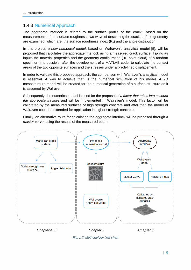
1.4.3 Numerical Approach The aggregate interlock is related to the surface profile of the crack. Based on the measurements of the surface roughness, two ways of describing the crack surface geometry are examined, which are: the surface roughness index (Rs) and the angle distribution.

In this project, a new numerical model, based on Walraven’s analytical model [5], will be proposed that calculates the aggregate interlock using a measured crack surface. Taking as inputs the material properties and the geometry configuration (3D point cloud) of a random specimen it is possible, after the development of a MATLAB code, to calculate the contact areas of the two opposite surfaces and the stresses under a predefined displacement.

In order to validate this proposed approach, the comparison with Walraven’s analytical model is essential. A way to achieve that, is the numerical simulation of his model. A 2D mesostructure model will be created for the numerical generation of a surface structure as it is assumed by Walraven.

Subsequently, the numerical model is used for the proposal of a factor that takes into account the aggregate fracture and will be implemented in Walraven’s model. This factor will be calibrated by the measured surfaces of high strength concrete and after that, the model of Walraven could be extended for application in higher strength concrete.

Finally, an alternative route for calculating the aggregate interlock will be proposed through a master curve, using the results of the measured beam.

Chapter 4, 5 Chapter 3 Chapter 6

Fig. 1.7: Methodology flow chart

1. Introduction

| 7

1.5 Thesis Outline The structure of this thesis is presented below.

Chapter 1 provides background information about the shear failure and the aggregate interlock mechanism. Also, the research objectives and the methodology that will be followed during this research will be reported.

Chapter 2 demonstrates an overview of the literature, which is related to this research. Many theoretical models for aggregate interlock mechanism are described, as well as relevant experimental work that is done through the years.

In Chapter 3 a numerical simulation of Walraven’s analytical model will be proposed and a validation of this proposed model will be performed.

Chapter 4 gives information about the experimental tests, the properties of the specimens and the method for the roughness measurement of the cracked surfaces from a laser scanner.

Chapter 5 explains the method for the post-processing of the laser scanning data and presents two ways of describing the roughness properties which are the surface roughness index (Rs) and the angle distribution.

Chapter 6 displays the results for the measured crack surfaces generated by the proposed numerical approach, which is described in detail at the beginning of the chapter. Also, a reduction factor that will be implemented into Walraven’s model and considers the aggregate fracture, is generated, based on the experimental results. Through a study of the measured beam, the goal of creating a master curve that will provide the aggregate interlock, will be reached.

Chapter 7 presents the main conclusions of this research and recommendations for further research on this subject.

1. Introduction

| 8

| 9

2 Literature Review

In order to obtain more insight of the mechanism of aggregate interlock, a literature study on the existing theoretical models is deemed necessary. In addition, the following gathering of the relevant experimental results is essential for the implementation of the project.

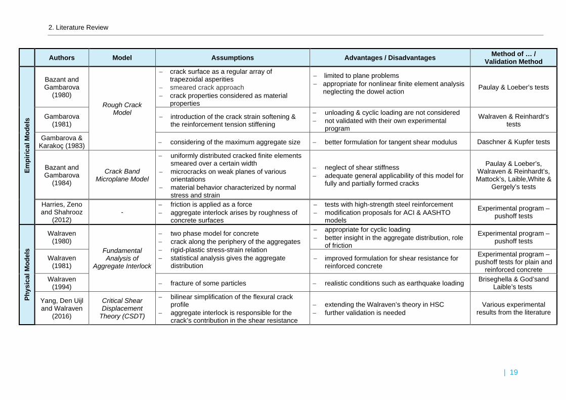
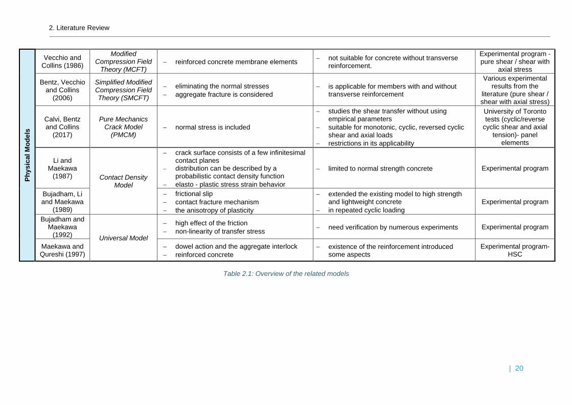
2.1 Theoretical Models In the last years, several models have been proposed for the description of the shear behavior considering the mechanism of aggregate interlock. In this section a review from 1980 until today will be demonstrated. Attention will be given to the assumptions, the advantages, the disadvantages, the principal equations and the validation method of each model. Also, the theoretical models are summarized in Table 2.1.

2.1.1 Empirical models The following models are based on regression analysis of experimental results.

Bažant and Gambarova (1980) presented the Rough Crack Model. In this approach, the crack slip of rough crack surfaces is directly related to the aggregate interlock. It is assumed that in-plane forces act in the concrete plate where the reinforcing bars as well as the cracks are densely distributed (Fig. 2.1- left). Also, only the axial stresses are considered to be carried from the reinforcing bars. The relation between normal and shear stresses, the crack opening and the crack slip is considered as a material property, which is expressed as the crack stiffness. The crack surface is simplified as a row of trapezoidal curves (Fig. 2.1- right). The numerical analysis required fitting of the results from the various types of tests (at constant crack width / constant confinement). Finally, the results of the derived equations were satisfactory precise compared to these of the existing experiments. This model is appropriate for nonlinear finite element analysis with a limitation to monotonic incremental loading neglecting the dowel action and the kinking of the bars [6].

Fig. 2.1: Rough crack model

2. Literature Review

| 10

Two important parameters were missing from this model. Therefore, a year later, Gambarova (1981) proposed the introduction of the crack strain softening and the reinforcement tension stiffening, improving the existing approach. The strain softening explains the fact that the stresses become zero, when the crack faces lose contact. On the other hand, the tension stiffening considers the effect of bond between reinforcement and concrete increasing the crack shear stiffness. However, the establishment of these improvements was not validated due to some weaknesses in the existing experiments, which are related to these parameters. Results by Walraven and Reinhardt were used for the validation [7].

Gambarova & Karakoç (1983) improved the Rough Crack model based on tests only with constant confinement. The relation between the normal stress and the crack displacements changed considering the maximum aggregate size. The resulting better formulation for tangent shear modulus of cracked concrete facilitates significantly the finite element analysis [8].

A new model more suitable for finite element analysis was performed by Bazant and Gambarova (1984) based on data from various shear tests. The Crack Band Microplane Model assumes uniformly distributed cracked finite elements smeared over a certain width. This was an already known approach, namely crack band theory, but the introduction of microplane model expanded it for the cases of arbitrary general loading path where microcracks are formed on weak planes of various orientations. It is concluded that the shear stiffness in each microplane could be neglected and the material behavior is characterized by the relation between the normal stress and strain for each micromodel. The smeared cracking overcomes the computational difficulties. In particular, at the line crack model there is an increase in the number of nodes when the crack line propagates, and trial calculations must be done for the prediction of the location of the nodes. On the other hand, the smeared cracking is a fixed mesh with certain number of nodes. Into these benefits the adequate general applicability of this model for fully and partially formed cracks, is added, which is proven by the comparison with many experimental data from the literature [9].

One more empirically derived model explaining the aggregate interlock in reinforced concrete was accomplished recently by Harries, Zeno and Shahrooz (2012). The ACI and AASHTO LFRD provisions about this topic were studied and a new modified model that represents better the actual behavior was proposed based on them. It was shown that these provisions are unreliable because they are based on data for lower strength of reinforcing steel and concrete compared to these that are used nowadays. For this reason, a special experimental study that included push-off tests with high-strength steel reinforcement have been done in addition to some existing data that were used. The outcome showed that the aggregate interlock mechanism is divided into 3 important stages: the precracked, the postcracked and the post-ultimate behavior. Therefore, a new expression for the shear friction was proposed (2.3) including the concrete contribution, which is significant in the precracked stage and the friction force by the reinforcement that affects the following stages. In addition, the ACI and AASHTO approaches wrongly assume, as the past models, that the reinforcement steel yields when the ultimate capacity is reached, so the steel strength is considered to be equal to the yield strength. However, these experimental results showed that the ultimate capacity occurs before the yielding of the reinforcement and the friction force is a function of the steel modulus [10]. The aforementioned differences can be observed below, where the proposed modified equation (2.3) as well as the existing equations (2.1)(2.2) for the shear friction capacity by ACI and AASHTO are depicted.


| 11

𝐴𝐴𝐴𝐴𝐴𝐴𝐴𝐴𝐴𝐴𝐴𝐴: 𝑉𝑉𝑚𝑚𝑚𝑚 = 𝑐𝑐 ∙ 𝐴𝐴𝑐𝑐𝑣𝑣 + 𝜇𝜇 ∙ (𝐴𝐴𝑣𝑣𝑣𝑣𝐶𝐶𝑦𝑦 + 𝑃𝑃𝑐𝑐) (2.1)

𝐴𝐴𝐶𝐶𝐴𝐴: 𝑉𝑉𝑚𝑚𝑚𝑚 = 𝐴𝐴𝑣𝑣𝑣𝑣 ∙ 𝐶𝐶𝑦𝑦 ∙ 𝜇𝜇 (2.2)

𝑉𝑉𝑚𝑚𝑚𝑚 = 𝑎𝑎 ∙ 𝐴𝐴𝑐𝑐𝑣𝑣 ∙ 𝐶𝐶𝑐𝑐𝑚𝑚 + 0.002 ∙ 𝐴𝐴𝑣𝑣𝑣𝑣 ∙ 𝐸𝐸𝑠𝑠 ≤ 0.02𝐴𝐴𝑐𝑐𝑣𝑣 ∙ 𝐶𝐶′𝑐𝑐 (2.3)

Where,

𝐴𝐴𝑐𝑐𝑣𝑣: area of concrete shear interface

𝐴𝐴𝑣𝑣𝑣𝑣: area of interface shear reinforcement

𝜇𝜇 : coefficient of friction

𝑐𝑐 : cohesion factor

𝑃𝑃𝑐𝑐: permanent net compressive strength

𝑎𝑎: coefficient for interface / pre-crack condition

𝐸𝐸𝑠𝑠: Young’s modulus of steel

2.1.2 Physical models The following two basic models and their modifications will be further investigated in the project. These are two micro-physical models based on assumptions of the shape of the crack surface using rational formulation.

2.1.2.1 Walraven’s model and modifications based on this

The rational and remarkably detailed explanation of the aggregate interlock by Walraven made his model the basis for many investigations and development of new improved models. Also, this research will be based on this.

After a thorough study from Walraven (1980), the Fundamental Analysis of Aggregate Interlock was occurred. This physical model distinguishes concrete in two phases: the aggregate particles, which are simplified as spheres with higher strength and a matrix consisting of hardened cement paste with lower strength. The aggregate grading was taken also into account. The crack behavior is simply explained as friction between two interfaces and the crack expands along the periphery of the aggregate spheres (Fig. 2.2).

Fig. 2.2: Walraven’ s model


| 12

The shear and the normal stresses are developed during the shear displacement and the sliding of the formed contact areas. The relation between normal stresses and strains is assumed as rigid-plastic. Moreover, the model includes a statistical analysis in order to calculate the distribution of the particles on the crack plane, in particular the depth that aggregate embeds into the crack surface. Various tests demonstrated the variables that influence the aggregate interlock. Some of them are the aggregate size, the type of grading curve, the friction, the loading protocol (monotonic / cycling). The expressions for the normal and shear stress are the following (2.4). The contact areas depend on the crack width (w), the shear displacement (Δ), the maximum diameter of the aggregates and the aggregate volume [11] [12].

𝜎𝜎 = 𝜎𝜎𝑝𝑝𝑝𝑝 ∙ ��̅�𝐴𝑥𝑥 − 𝜇𝜇 ∙ �̅�𝐴𝑦𝑦� 𝜏𝜏 = 𝜎𝜎𝑝𝑝𝑝𝑝 ∙ (�̅�𝐴𝑦𝑦 + 𝜇𝜇 ∙ �̅�𝐴𝑥𝑥)

(2.4)

Where, 𝜎𝜎 : normal stress at the crack surface 𝜏𝜏 : shear stress at the crack surface 𝜎𝜎𝑝𝑝𝑝𝑝 = 6.39𝐶𝐶′𝑐𝑐𝑐𝑐

0.56 : matrix yielding strength 𝐶𝐶′𝑐𝑐𝑐𝑐 : crushing strength of cement matrix �̅�𝐴𝑥𝑥 : projection of total contact area on x-plane �̅�𝐴 𝑦𝑦 : projection of total contact area on y-plane Case A: 𝛥𝛥 < 𝑤𝑤

�̅�𝐴𝑦𝑦 = � 𝑝𝑝𝑐𝑐 ∙4𝜋𝜋∙ 𝐹𝐹 �

𝐷𝐷𝐷𝐷𝑚𝑚𝑚𝑚𝑥𝑥

� ∙ 𝐺𝐺1(𝛥𝛥,𝑤𝑤,𝐷𝐷)𝐷𝐷𝑚𝑚𝑚𝑚𝑥𝑥

𝑤𝑤2+𝛥𝛥2𝛥𝛥

∙ 𝑑𝑑𝐷𝐷

�̅�𝐴𝑥𝑥 = � 𝑝𝑝𝑐𝑐 ∙4𝜋𝜋∙ 𝐹𝐹 �



𝑤𝑤2+𝛥𝛥2𝛥𝛥


Case B: 𝛥𝛥 < 𝑤𝑤

�̅�𝐴𝑦𝑦 = � 𝑝𝑝𝑐𝑐 ∙4𝜋𝜋∙ 𝐹𝐹 �


� ∙ 𝐺𝐺3(𝛥𝛥,𝑤𝑤,𝐷𝐷)𝑤𝑤2+𝛥𝛥2𝑤𝑤

2𝑤𝑤∙ 𝑑𝑑𝐷𝐷 + � 𝑝𝑝𝑐𝑐 ∙

4𝜋𝜋∙ 𝐹𝐹 �



𝑤𝑤2+𝛥𝛥2𝑤𝑤


�̅�𝐴𝑥𝑥 = � 𝑝𝑝𝑐𝑐 ∙4𝜋𝜋∙ 𝐹𝐹 �


� ∙ 𝐺𝐺4(𝛥𝛥,𝑤𝑤,𝐷𝐷)𝑤𝑤2+𝛥𝛥2𝑤𝑤

2𝑤𝑤∙ 𝑑𝑑𝐷𝐷 + � 𝑝𝑝𝑐𝑐 ∙

4𝜋𝜋∙ 𝐹𝐹 �



𝑤𝑤2+𝛥𝛥2𝑤𝑤



| 13

Where,

𝐹𝐹 �𝐷𝐷

𝐷𝐷𝑚𝑚𝑚𝑚𝑥𝑥� = 0.532 ∙ �

𝐷𝐷𝐷𝐷𝑚𝑚𝑎𝑎𝐷𝐷

�0.5

− 0.212 ∙ �𝐷𝐷

𝐷𝐷𝑚𝑚𝑎𝑎𝐷𝐷�4

− 0.072 ∙ �𝐷𝐷


− 0.036 ∙ �𝐷𝐷


− 0.025

∙ �𝐷𝐷


𝑢𝑢𝑚𝑚𝑚𝑚𝑥𝑥 =− 1

2𝑤𝑤(𝑤𝑤2 + 𝛥𝛥2) + 12�𝑤𝑤

2(𝑤𝑤2 + 𝛥𝛥2)2 − (𝑤𝑤2 + 𝛥𝛥2) ∙ ((𝑤𝑤2 + 𝛥𝛥2)2 − 4𝛥𝛥2𝑅𝑅2)𝑤𝑤2 + 𝛥𝛥2

𝐺𝐺1(𝛥𝛥,𝑤𝑤,𝐷𝐷) = 𝐷𝐷−3 ∙ ��𝐷𝐷2 − (𝑤𝑤2 + 𝛥𝛥2)𝛥𝛥

√𝑤𝑤2 + 𝛥𝛥2∙ 𝑢𝑢𝑚𝑚𝑚𝑚𝑥𝑥 − 𝑤𝑤 ∙ 𝑢𝑢𝑚𝑚𝑚𝑚𝑥𝑥 − 𝑢𝑢𝑚𝑚𝑚𝑚𝑥𝑥2�

𝐺𝐺2(𝛥𝛥,𝑤𝑤,𝐷𝐷) =

𝐷𝐷−3 ∙ ��𝛥𝛥 − �𝐷𝐷2 − (𝑤𝑤2 + 𝛥𝛥2)𝑤𝑤

√𝑤𝑤2 + 𝛥𝛥2� ∙ 𝑢𝑢𝑚𝑚𝑚𝑚𝑥𝑥 − (𝑤𝑤 + 𝑢𝑢𝑚𝑚𝑚𝑚𝑥𝑥) ∙ �

14∙ 𝐷𝐷2 − (𝑤𝑤 + 𝑢𝑢𝑚𝑚𝑚𝑚𝑥𝑥)2

− 𝑤𝑤�14∙ 𝐷𝐷2 − 𝑤𝑤2 +

14∙ 𝐷𝐷2𝑎𝑎𝑎𝑎𝑐𝑐𝑠𝑠𝑎𝑎𝑛𝑛 �

𝑤𝑤 + 𝑢𝑢𝑚𝑚𝑚𝑚𝑥𝑥12𝐷𝐷

� −14∙ 𝐷𝐷2𝑎𝑎𝑎𝑎𝑐𝑐𝑠𝑠𝑎𝑎𝑛𝑛 �

2𝑤𝑤𝐷𝐷��

𝐺𝐺3(𝛥𝛥,𝑤𝑤,𝐷𝐷) = 𝐷𝐷−3 �12𝐷𝐷 − 𝑤𝑤�

2

𝐺𝐺4(𝛥𝛥,𝑤𝑤,𝐷𝐷) = 𝐷𝐷−3 �𝜋𝜋8𝐷𝐷2 − 𝑤𝑤�

14𝐷𝐷2 − 𝑤𝑤2 −

14∙ 𝐷𝐷2𝑎𝑎𝑎𝑎𝑐𝑐𝑠𝑠𝑎𝑎𝑛𝑛 �

2𝑤𝑤𝐷𝐷��

Many tests have been carried out by the same author in 1981 for plain and reinforced concrete that prove the reliability of this approach. The results from the theory reached more precisely the experimental due to a correction for the elastic deformations which were neglected because the plastic considered as dominant. At the same time the difference in behavior between them, due to the bond stresses between concrete and reinforcement, became apparent. However, a significant disadvantage is that the model and the experiments were limited to a low strength of concrete up to 60 N/mm2 [5].

In 1994, Walraven adjusted his model to more realistic conditions such as earthquake loading. The representation of the aggregates as spheres, the assumption that the matrix behaves like a rigid-plastic material and the formulas remain the same. However, one parameter is added in the existing model. As it is expected, fracture of some particles will occur in high strength or in concrete with low-strength aggregates. Therefore, the fracture index (𝐶𝐶𝑣𝑣) was introduced as a material parameter that reduces the total projected contact areas (2.6). It was concluded that fracture and friction are decisive parameters for cyclic loading. The validation of the model was achieved through comparison with experiments of other authors [13].

𝜎𝜎 = 𝐶𝐶𝑣𝑣 ∙ 𝜎𝜎𝑝𝑝𝑝𝑝 ∙ ��̅�𝐴𝑥𝑥 − 𝜇𝜇 ∙ �̅�𝐴𝑦𝑦� 𝜏𝜏 = 𝐶𝐶𝑣𝑣 ∙ 𝜎𝜎𝑝𝑝𝑝𝑝 ∙ (�̅�𝐴𝑦𝑦 + 𝜇𝜇 ∙ �̅�𝐴𝑥𝑥)

(2.5)


| 14

In 2016, Yang, Den Uijl and Walraven developed the Critical Shear Displacement Theory (CSDT). This model aims to the evolution of shear design for high-strength concrete members without shear reinforcement. Two failure modes were depicted: the flexural shear and the shear compression. The flexural shear failure gives a lower bound for shear capacity. Therefore, an expression for the critical shear displacement, which is the value of the initiation of the unstable flexural crack, was determined based on a big number of experimental data. Between the assumptions that were made the most significant is the bilinear simplification of the flexural crack profile and the assumption that the aggregate interlock in the main branch is responsible for the crack’s contribution in the shear resistance [1]. Regarding the aggregate interlock mechanism, the authors improved the Walraven's model considering the fact that in high strength concrete the aggregate particles fracture, so the contact area reduces and as a result the shear stress that can be carried by aggregate interlock reduces too. For this reason, they introduced a reduction factor (𝑅𝑅𝑚𝑚𝑚𝑚) in the shear stress formula that taking into account the aggregate interlock, as it is depicted in the equation (2.6). This model seems to be reliable compared to a limited number of experimental results. However, further validation is needed which will consider the fracture of the aggregates [14].

𝜏𝜏 = 𝑅𝑅𝑚𝑚𝑚𝑚 ∙ 𝜎𝜎𝑝𝑝𝑝𝑝 ∙ (�̅�𝐴𝑦𝑦 + 𝜇𝜇 ∙ �̅�𝐴𝑥𝑥) (2.6)

Where,

𝑅𝑅𝑚𝑚𝑚𝑚 = 0.85��7.2

𝐶𝐶𝑐𝑐𝑚𝑚 − 40 + 1�2

− 1 + 0.34 (2.7)

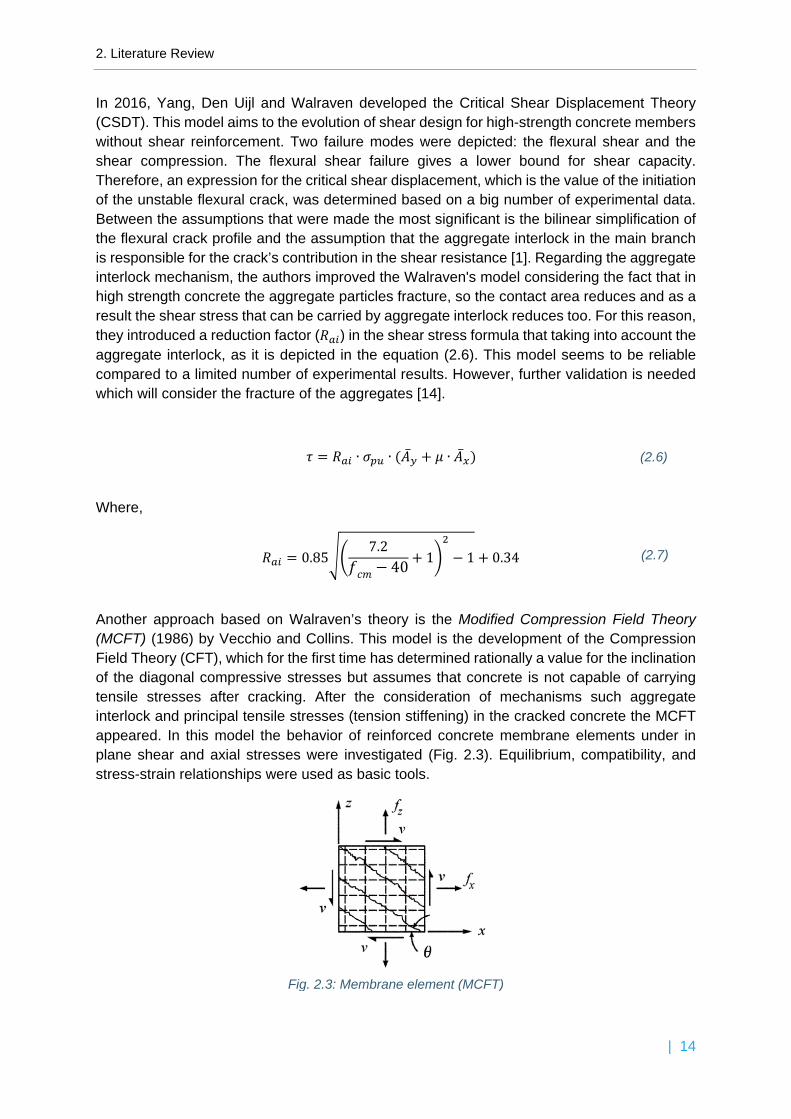
Another approach based on Walraven’s theory is the Modified Compression Field Theory (MCFT) (1986) by Vecchio and Collins. This model is the development of the Compression Field Theory (CFT), which for the first time has determined rationally a value for the inclination of the diagonal compressive stresses but assumes that concrete is not capable of carrying tensile stresses after cracking. After the consideration of mechanisms such aggregate interlock and principal tensile stresses (tension stiffening) in the cracked concrete the MCFT appeared. In this model the behavior of reinforced concrete membrane elements under in plane shear and axial stresses were investigated (Fig. 2.3). Equilibrium, compatibility, and stress-strain relationships were used as basic tools.

Fig. 2.3: Membrane element (MCFT)


| 15

Based on Walraven’s model the authors derived the following equation [15]:

𝜏𝜏 = 0,18𝜏𝜏𝑚𝑚𝑚𝑚𝑥𝑥 + 1,64𝜎𝜎 −0,82𝜎𝜎2

𝜏𝜏𝑚𝑚𝑚𝑚𝑥𝑥 (2.8)

Where,

𝜏𝜏𝑚𝑚𝑚𝑚𝑥𝑥 =�𝐶𝐶𝑐𝑐𝑚𝑚

0.31 + 24𝑤𝑤𝐷𝐷𝑚𝑚𝑚𝑚𝑥𝑥 + 16

(2.9)

𝜏𝜏𝑚𝑚𝑚𝑚𝑥𝑥 : maximum shear stress that can be resisted by aggregate interlock 𝐷𝐷𝑚𝑚𝑚𝑚𝑥𝑥 : maximum aggregate size

It is observed from the formula that the shear displacement (Δ) does not affect the shear stress, fact which is not realistic according to the existing reliable models. Therefore, this model is not suitable for concrete without transverse reinforcement.

In 2006 the Simplified Modified Compression Field Theory (SMCFT) was presented by Bentz, Vecchio and Collins. The SMCFT is based on the results of 102 shear tests on reinforced concrete panels. This model can predict accurately the shear strength eliminating the normal stresses and using only simple equations for the inclination of diagonal compressive stresses (θ) and the factor for tensile stresses (β). Also, the aggregate fracture is considered for high strength concrete setting as zero the term that represents the maximum aggregate size when the concrete strength is fcm > 70 MPa. But this assumption introduces a steep decrease of the shear capacity which is not so realistic. In addition, the model is applicable for members with and without transverse reinforcement. It seems to give more conservative results but at the same time gives excellent predictions of shear strength. The factor 𝛽𝛽 depends on the crack width as well as the final equation for shear capacity as it is shown (2.10) [16]:

𝜏𝜏 = 𝛽𝛽 ∙ �𝐶𝐶𝑐𝑐𝑚𝑚 (2.10)

Where, 𝜏𝜏 : shear stress at the crack surface 𝛽𝛽 : factor for tensile stresses An interesting approach by the same authors was demonstrated in 2017. Calvi, Bentz and Collins presented the Pure Mechanics Crack Model (PMCM), an improved version of their own previous models. The main advantage of this model is that studies the shear transfer in cracked reinforced concrete without using empirical parameters, but it requires only some basic properties of the structure as it is obvious from the formula of shear stress:

𝜏𝜏 =𝜌𝜌𝑠𝑠 ∙ 𝐶𝐶𝑦𝑦,𝑐𝑐𝑟𝑟 ∙ (𝑤𝑤 + 𝜇𝜇 ∙ 𝛥𝛥)

𝛥𝛥 − 𝜇𝜇 ∙ 𝑤𝑤 + 𝑛𝑛 ∙ 𝑤𝑤 + 𝑛𝑛 ∙ 𝜇𝜇 ∙ 𝛥𝛥 (2.11)

Where,

𝜏𝜏 : shear stress at the crack surface


| 16

𝜌𝜌𝑠𝑠 : longitudinal reinforcement ratio

𝐶𝐶𝑦𝑦,𝑐𝑐𝑟𝑟 : tensile stress in longitudinal reinforcement at the crack surface

𝛥𝛥 : crack slip

𝑛𝑛 : tension-to-shear loading ratio

Also, the included normal stress makes the model more realistic than before. The equilibrium, compatibility and constitutive equations that are used, make the model applicable for various loading conditions. The equilibrium equations differ for the loading, the unloading and the reverse loading phases, as long as the forces change direction. This model is suitable for monotonic, cyclic, reversed cyclic shear and axial loads. However, there are restrictions in its applicability due to the specific demand of the orientation of the reinforcement and the usage of an unknown value for the length of the reinforcement. Therefore, generalization and validation are needed for a future implementation of the model [17].

2.1.2.2 Contact density model and modifications

The Contact Density Model by Li and Maekawa (1987) introduced the geometrical roughness and the mechanical rigidity of crack faces. This physical approach is based on the following three assumptions. It assumes that the crack surface consists of a few infinitesimal contact planes with various inclinations (Fig. 2.4a). This distribution can be described by a probabilistic contact density function which is independent of the size and the grading of the aggregates (Fig. 2.4b). Also, the contact stress transfer is calculated based on an elasto-perfectly plastic model (Fig. 2.4c) and is the result of the integration of all the local stresses at each contact plane.

These assumptions make the model suitable for application in cycling and non-proportional loading. The verification was accomplished through systematically planned experimental process. However, its applicability is limited to normal strength concrete [18]. Below, the expressions for shear and normal stress are demonstrated.

a) Idealization of crack surface b) Contact density function c) Contact stress model

Fig. 2.4: Contact Density Model


| 17

𝜏𝜏 = � 𝑅𝑅𝑐𝑐(𝑤𝑤,𝛥𝛥,𝜃𝜃) ∙ 𝑠𝑠𝑎𝑎𝑛𝑛𝜃𝜃 𝑑𝑑𝜃𝜃𝜋𝜋/2

−𝜋𝜋/2= � 𝛢𝛢𝑡𝑡 ∙ 𝜎𝜎𝑐𝑐𝑐𝑐𝑚𝑚(𝜃𝜃) ∙ 𝐾𝐾(𝑤𝑤) ∙ 𝛺𝛺(𝜃𝜃) ∙ 𝑠𝑠𝑎𝑎𝑛𝑛𝜃𝜃 𝑑𝑑𝜃𝜃

𝜋𝜋/2

−𝜋𝜋/2 (2.12)

𝜎𝜎 = � 𝑅𝑅𝑐𝑐(𝑤𝑤,𝛥𝛥, 𝜃𝜃) ∙ 𝑐𝑐𝑐𝑐𝑠𝑠𝜃𝜃 𝑑𝑑𝜃𝜃𝜋𝜋/2

−𝜋𝜋/2= � 𝛢𝛢𝑡𝑡 ∙ 𝜎𝜎𝑐𝑐𝑐𝑐𝑚𝑚(𝜃𝜃) ∙ 𝐾𝐾(𝑤𝑤) ∙ 𝛺𝛺(𝜃𝜃) ∙ 𝑠𝑠𝑎𝑎𝑛𝑛𝜃𝜃 𝑑𝑑𝜃𝜃

𝜋𝜋/2

−𝜋𝜋/2 (2.13)

Where,

𝑅𝑅𝑐𝑐 : contact normal force

𝜃𝜃 : angle of contact stress

𝛢𝛢𝑡𝑡 : total area of crack surface

𝜎𝜎𝑐𝑐𝑐𝑐𝑚𝑚(𝜃𝜃) : contact stress

𝐾𝐾(𝑤𝑤) : ratio of effective contact area

𝛺𝛺(𝜃𝜃) : contact density function

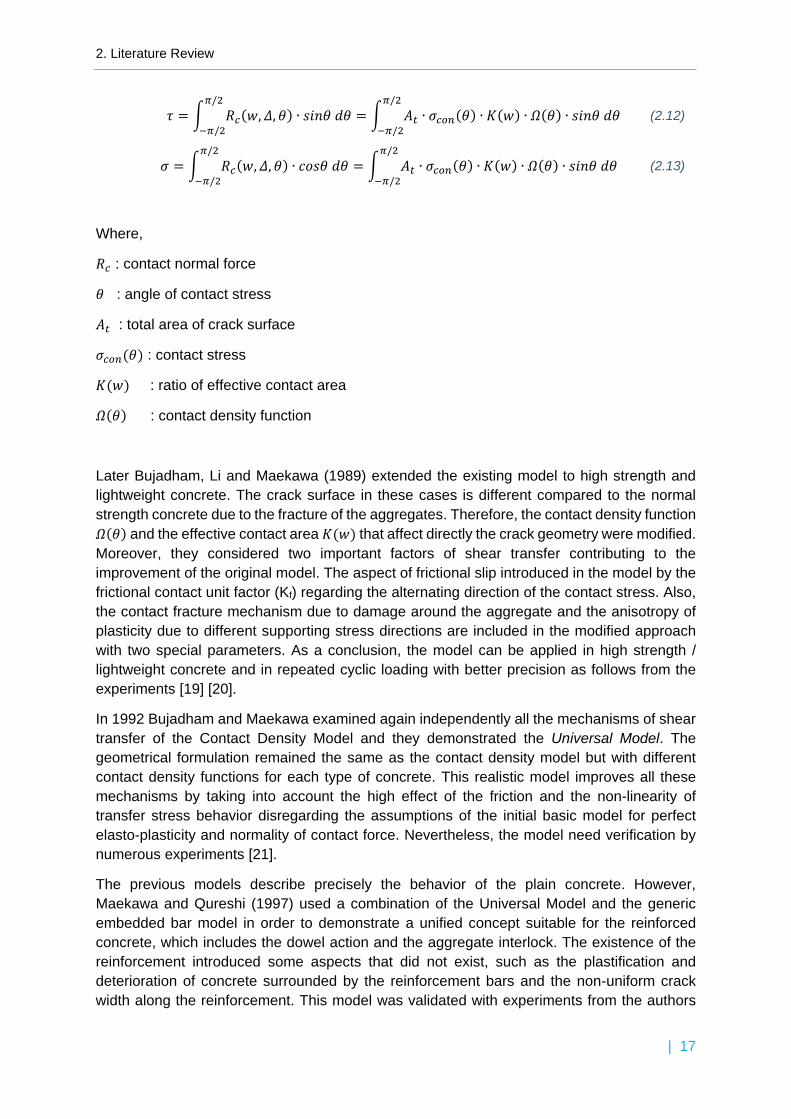
Later Bujadham, Li and Maekawa (1989) extended the existing model to high strength and lightweight concrete. The crack surface in these cases is different compared to the normal strength concrete due to the fracture of the aggregates. Therefore, the contact density function 𝛺𝛺(𝜃𝜃) and the effective contact area 𝐾𝐾(𝑤𝑤) that affect directly the crack geometry were modified. Moreover, they considered two important factors of shear transfer contributing to the improvement of the original model. The aspect of frictional slip introduced in the model by the frictional contact unit factor (Kf) regarding the alternating direction of the contact stress. Also, the contact fracture mechanism due to damage around the aggregate and the anisotropy of plasticity due to different supporting stress directions are included in the modified approach with two special parameters. As a conclusion, the model can be applied in high strength / lightweight concrete and in repeated cyclic loading with better precision as follows from the experiments [19] [20].

In 1992 Bujadham and Maekawa examined again independently all the mechanisms of shear transfer of the Contact Density Model and they demonstrated the Universal Model. The geometrical formulation remained the same as the contact density model but with different contact density functions for each type of concrete. This realistic model improves all these mechanisms by taking into account the high effect of the friction and the non-linearity of transfer stress behavior disregarding the assumptions of the initial basic model for perfect elasto-plasticity and normality of contact force. Nevertheless, the model need verification by numerous experiments [21].

The previous models describe precisely the behavior of the plain concrete. However, Maekawa and Qureshi (1997) used a combination of the Universal Model and the generic embedded bar model in order to demonstrate a unified concept suitable for the reinforced concrete, which includes the dowel action and the aggregate interlock. The existence of the reinforcement introduced some aspects that did not exist, such as the plastification and deterioration of concrete surrounded by the reinforcement bars and the non-uniform crack width along the reinforcement. This model was validated with experiments from the authors


| 18

and from the literature. In addition, the reinforcement ratio effect and size effect were investigated concluding that the increasing ratio increases the contribution of shear transfer mechanisms in the shear transfer and the size does not affect significantly the shear transfer [22].


| 19

Authors Model Assumptions Advantages / Disadvantages Method of … / Validation Method

Empi

rical

Mod

els

Bazant and Gambarova

(1980) Rough Crack

Model

− crack surface as a regular array of trapezoidal asperities

− smeared crack approach − crack properties considered as material

properties

− limited to plane problems − appropriate for nonlinear finite element analysis

neglecting the dowel action

Paulay & Loeber’s tests

Gambarova (1981)

− introduction of the crack strain softening & the reinforcement tension stiffening

− unloading & cyclic loading are not considered − not validated with their own experimental

program

Walraven & Reinhardt’s tests

Gambarova & Karakoç (1983) − considering of the maximum aggregate size − better formulation for tangent shear modulus Daschner & Kupfer tests

Bazant and Gambarova

(1984)

Crack Band Microplane Model

− uniformly distributed cracked finite elements smeared over a certain width

− microcracks on weak planes of various orientations

− material behavior characterized by normal stress and strain

− neglect of shear stiffness − adequate general applicability of this model for

fully and partially formed cracks

Paulay & Loeber’s, Walraven & Reinhardt’s, Mattock’s, Laible,White &

Gergely’s tests

Harries, Zeno and Shahrooz

(2012) -

− friction is applied as a force − aggregate interlock arises by roughness of

concrete surfaces

− tests with high-strength steel reinforcement − modification proposals for ACI & AASHTO

models

Experimental program – pushoff tests

Phys

ical

Mod

els

Walraven (1980)

Fundamental Analysis of

Aggregate Interlock

− two phase model for concrete − crack along the periphery of the aggregates − rigid-plastic stress-strain relation − statistical analysis gives the aggregate

distribution

− appropriate for cyclic loading − better insight in the aggregate distribution, role

of friction

Experimental program – pushoff tests

Walraven (1981)

− improved formulation for shear resistance for reinforced concrete

Experimental program – pushoff tests for plain and

reinforced concrete Walraven

(1994) − fracture of some particles − realistic conditions such as earthquake loading Briseghella & God’sand Laible’s tests)

Yang, Den Uijl and Walraven

(2016)

Critical Shear Displacement

Theory (CSDT)

− bilinear simplification of the flexural crack profile

− aggregate interlock is responsible for the crack’s contribution in the shear resistance

− extending the Walraven’s theory in HSC − further validation is needed

Various experimental results from the literature


| 20

Phys

ical

Mod

els

Vecchio and Collins (1986)

Modified Compression Field

Theory (MCFT) − reinforced concrete membrane elements − not suitable for concrete without transverse

reinforcement.

Experimental program - pure shear / shear with

axial stress

Bentz, Vecchio and Collins

(2006)

Simplified Modified Compression Field Theory (SMCFT)

− eliminating the normal stresses − aggregate fracture is considered

− is applicable for members with and without transverse reinforcement

Various experimental results from the

literature (pure shear / shear with axial stress)

Calvi, Bentz and Collins

(2017)

Pure Mechanics Crack Model

(PMCM) − normal stress is included

− studies the shear transfer without using empirical parameters

− suitable for monotonic, cyclic, reversed cyclic shear and axial loads

− restrictions in its applicability

University of Toronto tests (cyclic/reverse

cyclic shear and axial tension)- panel

elements

Li and Maekawa

(1987) Contact Density Model

− crack surface consists of a few infinitesimal contact planes

− distribution can be described by a probabilistic contact density function

− elasto - plastic stress strain behavior

− limited to normal strength concrete Experimental program

Bujadham, Li and Maekawa

(1989)

− frictional slip − contact fracture mechanism − the anisotropy of plasticity

− extended the existing model to high strength and lightweight concrete

− in repeated cyclic loading Experimental program

Bujadham and Maekawa

(1992) Universal Model

− high effect of the friction − non-linearity of transfer stress − need verification by numerous experiments Experimental program

Maekawa and Qureshi (1997)

− dowel action and the aggregate interlock − reinforced concrete

− existence of the reinforcement introduced some aspects

Experimental program- HSC

Table 2.1: Overview of the related models


| 21

2.1.3 Conclusions All the above models show the complexity of the aggregate interlock mechanism. The common characteristic between all these models is the simulation of the stress transfer based on the crack surface geometry. Another one is the relation between the crack width, the shear displacement, the shear and the normal stress for the definition of the aggregate interlock mechanism. Among them, there are models such as the physical models that are based on the current knowledge, have a rational formulation and their results correspond to the experimental, in contrast to the empirical that are based on experimental results having limited applicability. However, the biggest percentage of the models are old and ignore the existence of new types of concrete such as high strength concrete. The most recent of them try to include this type of concrete but either need further validation or need some improvements, as it was discussed earlier.

2.2 Experimental Research Subsequently, it follows some experimental work that is done through the years. The purpose, the experimental program and the conclusions of each research will be presented.

Hamadi and Regan (1980) investigated the influence of different types of aggregate. They carried out tests with push-off specimens and beams composed of natural gravel and lightweight aggregates. At first, they performed some push-off tests using some specimens with embedded and other with external rebars. A bilinear shear strength relationship was assumed. The results demonstrated the great difference between the two types of aggregate and the significant influence of the crack roughness at interlock strength and behavior. The crack surface of the gravel concrete was rough, and the fracture occurred around the aggregates, while in the lightweight concrete the opposite happened. The strength seems to depend on normal stress and not on the crack width in contrast with stiffness which depends on the crack width and not on the normal stress. In addition, 10 reinforced concrete T-beams were tested and also there were differences in strength and behavior due to the different aggregates. Their behavior was analyzed based on a truss model which gave different values for the angle of the web compression for the two types of concrete. Moreover, the paper contains some expressions including stiffness of the interlock, but the rough approximations and the assumption that the aggregate interlock behaves linearly elastic make these inappropriate for use. However, the proposed equations for the ultimate shear resistance give satisfactory results [23].

Millard and Johnson (1984) accomplished a new type of tests in reinforced concrete which study separately the mechanisms of dowel action and the aggregate interlock in tensile cracking. For the aggregate interlock testing, on which this research will focus, the dowel stiffness was eliminated with a special construction of oversized ducts around the reinforcement. Two different concrete mixes with low strength concrete (35 / 55 MPa) were used. The parameters that investigated were the initial crack width, the strength of concrete and the stiffness normal to the crack plane. The results of the tests were compared with different theoretical models from the literature and the two-phase model of Walraven was proved to be the most accurate having only the negative requirement for knowledge of stiffness before its use, which is something that should be measured. The diagrams that compare the experimental results with the model, agree between the various specimens with


| 22

different reinforcement diameters, sizes and strengths as well as constant or increasing crack widths [24]. A year later (1985) the same authors reported further investigations by combining the contributions of the two mechanisms and by applying shear forces simultaneously with tensile forces. The results aim at the investigation of the crack widening, the tensile forces and the shear stiffness. Strain gauges and resin injection used for this purpose and 13 specimens with various strengths and reinforcement were tested. The comparison between the results of the two papers showed that different mechanisms do not occur. Nevertheless, the two mechanisms of aggregate interlock and dowel action interact and end up in slightly different values of strength and stiffness compare to the independently study of them, due to the local bond between the reinforcement and the concrete [25].

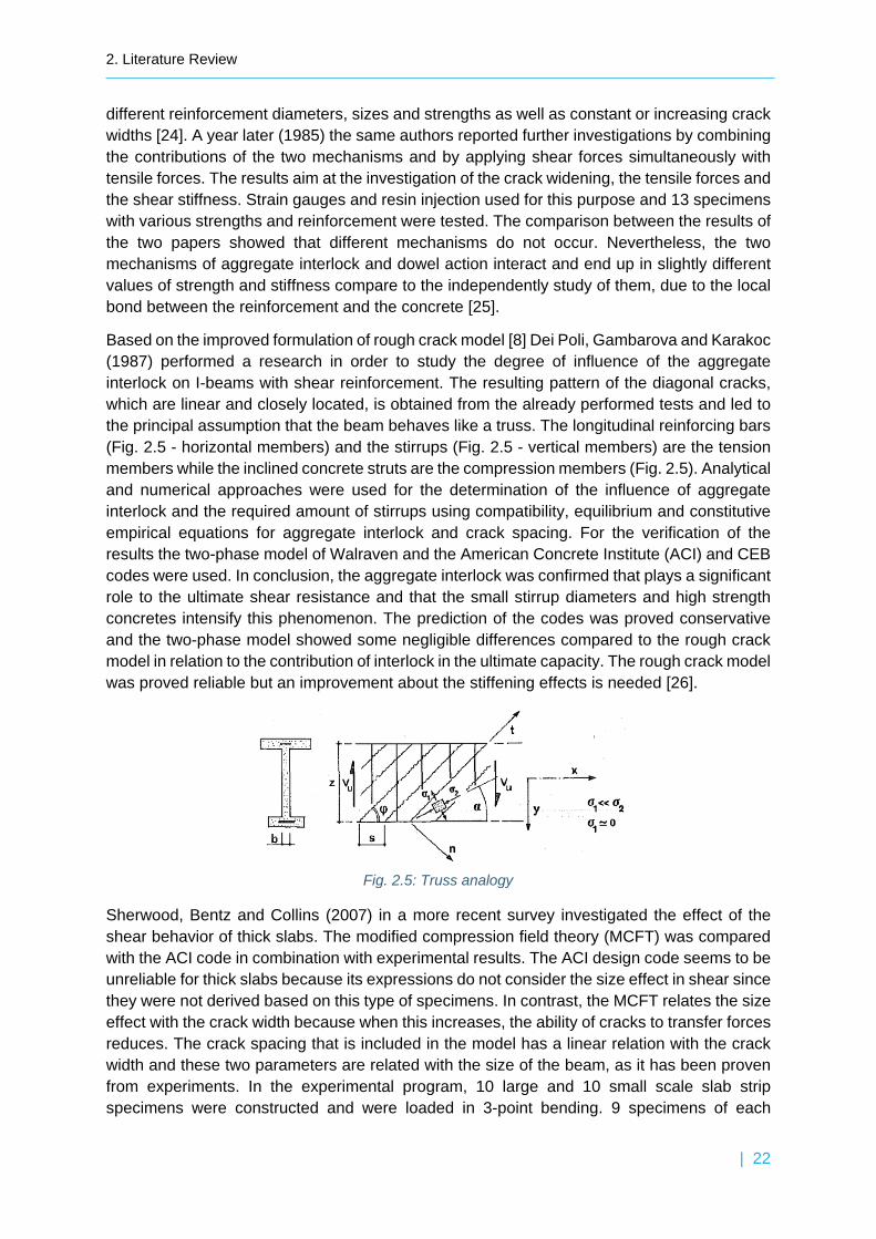
Based on the improved formulation of rough crack model [8] Dei Poli, Gambarova and Karakoc (1987) performed a research in order to study the degree of influence of the aggregate interlock on I-beams with shear reinforcement. The resulting pattern of the diagonal cracks, which are linear and closely located, is obtained from the already performed tests and led to the principal assumption that the beam behaves like a truss. The longitudinal reinforcing bars (Fig. 2.5 - horizontal members) and the stirrups (Fig. 2.5 - vertical members) are the tension members while the inclined concrete struts are the compression members (Fig. 2.5). Analytical and numerical approaches were used for the determination of the influence of aggregate interlock and the required amount of stirrups using compatibility, equilibrium and constitutive empirical equations for aggregate interlock and crack spacing. For the verification of the results the two-phase model of Walraven and the American Concrete Institute (ACI) and CEB codes were used. In conclusion, the aggregate interlock was confirmed that plays a significant role to the ultimate shear resistance and that the small stirrup diameters and high strength concretes intensify this phenomenon. The prediction of the codes was proved conservative and the two-phase model showed some negligible differences compared to the rough crack model in relation to the contribution of interlock in the ultimate capacity. The rough crack model was proved reliable but an improvement about the stiffening effects is needed [26].

Sherwood, Bentz and Collins (2007) in a more recent survey investigated the effect of the shear behavior of thick slabs. The modified compression field theory (MCFT) was compared with the ACI code in combination with experimental results. The ACI design code seems to be unreliable for thick slabs because its expressions do not consider the size effect in shear since they were not derived based on this type of specimens. In contrast, the MCFT relates the size effect with the crack width because when this increases, the ability of cracks to transfer forces reduces. The crack spacing that is included in the model has a linear relation with the crack width and these two parameters are related with the size of the beam, as it has been proven from experiments. In the experimental program, 10 large and 10 small scale slab strip specimens were constructed and were loaded in 3-point bending. 9 specimens of each

Fig. 2.5: Truss analogy


| 23

category did not have stirrups while only one had. Generally, there were specimens with different concrete strengths and maximum aggregate sizes. The outcome demonstrated the big influence of the aggregate interlock in shear and that the lack of it leads to failure. Also, it was presented that the maximum aggregate size affects significantly the shear capacity as long as the larger aggregates create rougher crack faces and as a result the aggregate interlock capacity increases. However, the high strength concrete specimens failed at a lower load due to the fracture of the aggregates. As expected, the ACI code overestimated the shear capacity of thick slabs and an improvement of the existing expression was proposed in order to provide safety. The MCFT was proved reliable and safe since it considers the size effect and the size and fracture of the aggregates, as it was mentioned. The brittle shear failure of all the members without shear reinforcement that was observed can be avoided with the application of a minimum quantity of stirrups as it is proposed in MCFT [27].

The research of Sagaseta and Vollum (2011) compared numerous analytical models, such as these of Hamadi and Regan (1980), Walraven and Reinhardt (1981), Gambarova and Karakoc (1983), the Simplified Contact Density Model (1989), the Modified Compression Field Theory (1986) and the MC90 (CEB-FIP,1990) in order to examine the influence of aggregate fracture through cracks in reinforced concrete. Various push-off tests were carried out and they were distinguished in two categories. There were specimens with gravel or limestone aggregates which are used in normal and high-strength concretes respectively. Very interesting remarks were occurred through the comparisons of the experimental and theoretical results. At first, the dowel action was neglected because its contribution was proven negligible. Regarding the shear stresses, the Hamadi and Regan and MC90 models predict satisfactorily the shear stress but after the first load cycle overestimate them. In contrast, the Walraven and Reinhardt and Gambarova and Karakoc models underestimate the shear and normal stresses for small shear displacements and overestimate them for larger shear displacements. They observed also that even though the fracture of the aggregates there was shear stress transfer due to the interlocking at macro-level. This means that the rough surfaces of the cracks create contact areas which allow the stress transfer. The authors also performed beam tests to slender and short-span beams using the same aggregate types as the push-off tests. They observed again the same phenomenon of transferring shear forces even with the fracture of the aggregates. However, they noticed that the aggregate fracture does not affect the strength of the beams with stirrups while decreased shear resistance in beams without stirrups was observed [28].

Cavagnis, Ruiz and Muttoni (2015) investigated the shear failure with a very different way. They examined the crack development and kinematics of beams during the failure using photogrammetric techniques. They used 13 normal strength concrete beams with variable length and as a result different slenderness. Also, the beams were tested under different loading conditions which correspond to reality. The crack patterns were observed in detail and different crack types were distinguished. The results displayed that many shear transfer mechanisms contribute to the shear strength and must be included in modelling of shear strength. However, the contribution of the aggregate interlock was proven, for one more time, significant considering the theoretical models and the resulting cracking patterns. Also, the aggregate interlock was observed that depends on geometry of the crack as it is already known. Finally, the authors propose the development of models which will take into account the development of cracking before and during failure [29].


| 24

In 2018 Huber T. presented a paper with title ‘Influence of aggregate interlock on the shear resistance of reinforced concrete beams without stirrups’, which demonstrates an approach similar to this project. For the purpose of this investigation, which was the quantification of the impact of concrete strength and properties, an experimental program was carried out. At first, splitting tests on specimens with different strengths (normal strength and self-compacting concrete) and different mixtures were done. The roughness of the remaining parts of these tests was measured with a laser microscope and the following relation between concrete strength and roughness was found.

𝑅𝑅𝑠𝑠 =2

𝐶𝐶𝑐𝑐1/8 (2.14)

Subsequently, 18 push-off tests were performed and the results of the normal and shear stresses and normal and shear displacements from LVDTs and digital image-correlation system were used for the derivation of a relationship between the aggregate effectivity factor from the fib Model Code and the roughness.

𝐶𝐶𝑣𝑣 =𝑅𝑅𝑠𝑠13.85

30 (2.15)

Also, 3 shear beam tests were performed, and the measurements of the kinematics were done in the same way. The deviations between them in the shear resistance revealed the big influence of the concrete mixture. Therefore, a modification of the Eurocode 2 formula was proposed, that takes into account the aggregate interlock and the type of mixture. Finally, it was concluded that, the aggregate interlock affects significantly the shear resistance [30].

2.2.1 Conclusions Generally, the experimental research proves the significant contribution of the aggregate interlock and surface roughness in shear. The variables that are used in almost every research were the concrete strength and the aggregate size. However, more research is needed about high strength concrete. Also, many models have been compared with the experimental results and their weaknesses revealed.

| 25 Fig. 3.1: Unacceptable conditions for aggregates [38]

a b c

3 Numerical simulation of Walraven’s model

In this chapter, a new approach for the numerical simulation of Walraven’s analytical model is proposed. The fundamental theory behind the model will be reserved, but it will be reproduced in a numerical way. The basic assumption of his model about the perfect plasticity of the material with a yield strength of σpu need to be verified whether is suitable for further use in the numerical approach. Also, another basic assumption is the certain structure for the crack surface. Therefore, the generation of such a structure, was the way to achieve that simulation. The construction of a numerical mesoscale model for concrete was developed, so a brief definition of this type of modelling is given. The assumptions that were adopted, followed by a detailed description of the process, are presented. Moreover, the procedure for the validation of the model, comparing the numerical and the analytical results, is analyzed. Finally, some results are shown as well as a discussion about them.

3.1 Definition of the numerical mesoscale modelling The mesoscale modelling could give a good insight of the mechanical behavior and the failure mechanisms of the large sized structures. A common way to generate a mesoscale model of concrete is the digital image processing. However, this approach requires the use of special equipment which is a costly and time-consuming procedure, because a large number of samples are usually needed for research purposes. On the other hand, computers nowadays provide unlimited possibilities. Taking advantage of this situation, it is possible to generate mesostructures for concrete, using algorithms. Many researchers have used this approach obtaining good results that correspond to the ones in real concrete and proving that this is a very practicable approach [31].

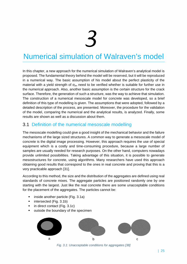
According to this method, the size and the distribution of the aggregates are defined using real standards of concrete mixes. The aggregate particles are positioned randomly one by one starting with the largest. Just like the real concrete there are some unacceptable conditions for the placement of the aggregates. The particles cannot be:

inside another particle (Fig. 3.1a) intersected (Fig. 3.1b) in direct contact (Fig. 3.1c) outside the boundary of the specimen

3. Numerical Approach

| 26

Fig. 3.2: Walraven’s model (left) Simulation of the model in MATLAB (right)

3.2 Numerical simulation The numerical simulation was achieved by performing a code in MATLAB software, which is attached in Appendix A.

3.2.1 Assumptions In order to reproduce Walraven’s model the following assumptions taken from the model itself are used:

− The aggregate particles are represented as circles − The matrix is a plastic material with yield strength equal to σpu − The aggregate distribution is determined by the Fuller curve, that represents a grading

of particles which results in an optimum density and strength. The cumulative

percentage passing a sieve is: 𝑃𝑃(𝐷𝐷) = � 𝐷𝐷𝐷𝐷𝑚𝑚𝑚𝑚𝑥𝑥

∙ 100

− The total area of the aggregates is taken as 75% of the concrete area (𝑝𝑝𝑐𝑐) − The crack propagation happens around the aggregates and not through them

More assumptions are used based on the literature [32]:

− The distance between the particles is taken as: 1.1 �𝐷𝐷𝐴𝐴+𝐷𝐷𝐵𝐵2

�, where 𝐷𝐷𝐴𝐴, 𝐷𝐷𝐵𝐵 are the diameters of 2 circles

3.2.2 Description of the procedure At first, a 2D mesostructure model is created with predefined dimensions. Only the coarse aggregates larger than 2 mm are modelled and the 4 larger sieve sizes are used from the aggregate grading curve. These 4 sieve sizes represent 4 different grading segments in the code. The procedure starts with the segment containing the largest diameters of the circles. The circles are placed one by one with a random diameter, only if all the requirements that are mentioned above are met. Each segment holds a certain percentage of area that has to be filled inside the specimen. When the required area is reached the procedure continues for the next segments until the aggregate area covers the 75% of the concrete area. For a better understanding, a flowchart of the algorithm of this procedure is depicted in Fig. 3.3. The outcome of this process is presented below (Fig. 3.2 – right). It is clear that the simulation is accurate enough compared to the original model by Walraven (Fig. 3.2 - left).


| 27

Fig. 3.3: Flowchart of the algorithm for the generation of the mesostructure in MATLAB

Legend

𝐴𝐴𝑛𝑛𝑝𝑝𝑢𝑢𝑡𝑡𝑠𝑠:

− Dimensions of the specimens − Aggregate area fraction pk − Size range of aggregates − Fuller curve

𝑛𝑛: number of grading segments (beginning from this with the largest diameters) 𝐴𝐴𝑎𝑎: the remaining area to be generated within a segment 𝐴𝐴𝑎𝑎: the area of each aggregate 𝐴𝐴𝑠𝑠: the area of the aggregates within a segment

As =𝑃𝑃(𝐷𝐷𝑚𝑚𝑚𝑚𝑥𝑥) − 𝑃𝑃(𝐷𝐷𝑚𝑚𝑚𝑚𝑚𝑚)𝑃𝑃(𝑑𝑑𝑚𝑚𝑚𝑚𝑥𝑥) − 𝑃𝑃(𝑑𝑑𝑚𝑚𝑚𝑚𝑚𝑚) ∙ 𝑝𝑝𝑐𝑐 ∙ 𝐴𝐴𝑐𝑐

Where,

𝐷𝐷𝑚𝑚𝑚𝑚𝑥𝑥/𝐷𝐷𝑚𝑚𝑚𝑚𝑚𝑚 : the maximum/minimum sizes of aggregate particles

𝑑𝑑𝑚𝑚𝑚𝑚𝑥𝑥/𝑑𝑑𝑚𝑚𝑚𝑚𝑚𝑚 : the maximum/minimum sizes of aggregate particles within a segment

𝑝𝑝𝑐𝑐: the aggregate area fraction

𝐴𝐴𝑐𝑐: the concrete area


| 28

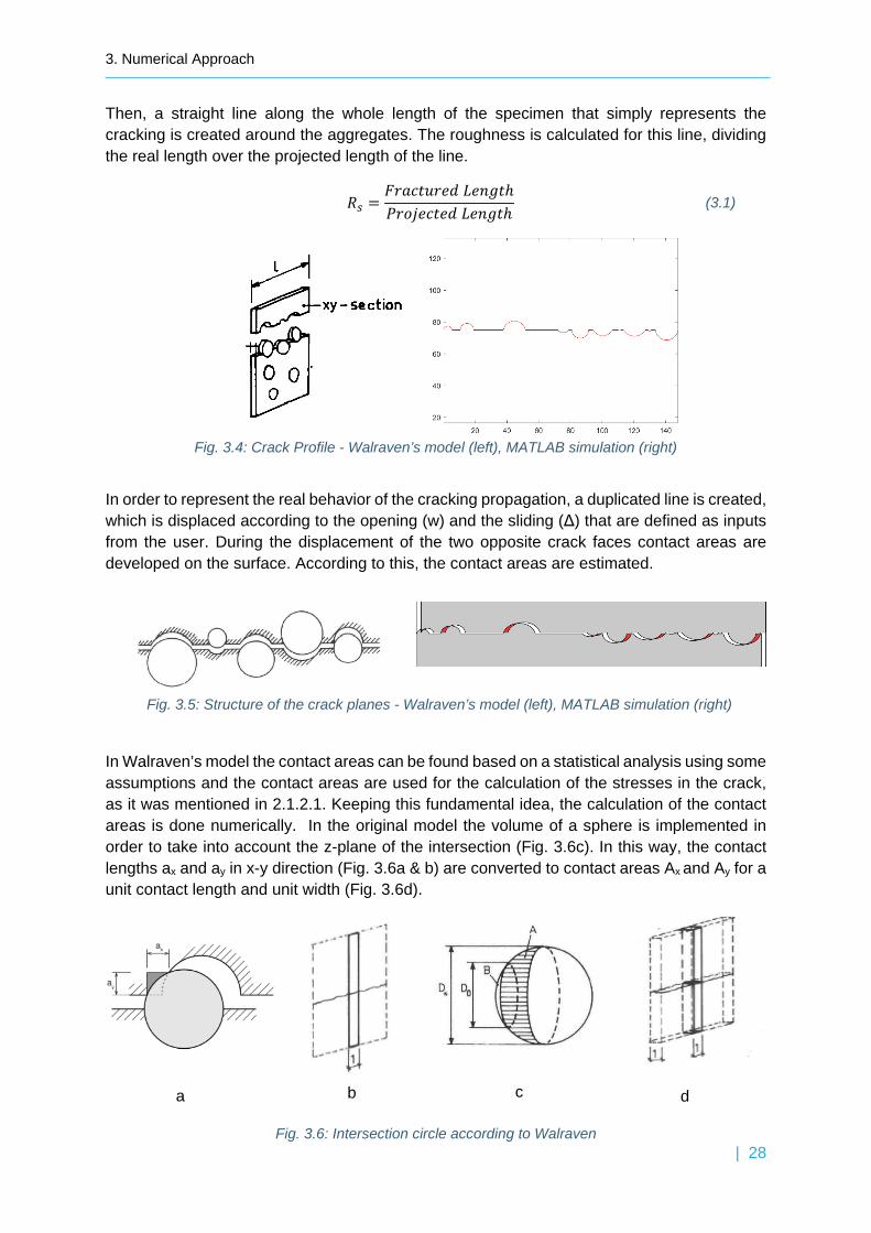
Then, a straight line along the whole length of the specimen that simply represents the cracking is created around the aggregates. The roughness is calculated for this line, dividing the real length over the projected length of the line.

𝑅𝑅𝑠𝑠 =𝐹𝐹𝑎𝑎𝑎𝑎𝑐𝑐𝑡𝑡𝑢𝑢𝑎𝑎𝐹𝐹𝑑𝑑 𝐿𝐿𝐹𝐹𝑛𝑛𝐿𝐿𝑡𝑡ℎ𝑃𝑃𝑎𝑎𝑐𝑐𝑃𝑃𝐹𝐹𝑐𝑐𝑡𝑡𝐹𝐹𝑑𝑑 𝐿𝐿𝐹𝐹𝑛𝑛𝐿𝐿𝑡𝑡ℎ

(3.1)

In order to represent the real behavior of the cracking propagation, a duplicated line is created, which is displaced according to the opening (w) and the sliding (Δ) that are defined as inputs from the user. During the displacement of the two opposite crack faces contact areas are developed on the surface. According to this, the contact areas are estimated.

In Walraven’s model the contact areas can be found based on a statistical analysis using some assumptions and the contact areas are used for the calculation of the stresses in the crack, as it was mentioned in 2.1.2.1. Keeping this fundamental idea, the calculation of the contact areas is done numerically. In the original model the volume of a sphere is implemented in order to take into account the z-plane of the intersection (Fig. 3.6c). In this way, the contact lengths ax and ay in x-y direction (Fig. 3.6a & b) are converted to contact areas Ax and Ay for a unit contact length and unit width (Fig. 3.6d).

Fig. 3.4: Crack Profile - Walraven’s model (left), MATLAB simulation (right)

Fig. 3.5: Structure of the crack planes - Walraven’s model (left), MATLAB simulation (right)

Fig. 3.6: Intersection circle according to Walraven

a c d b


| 29

Two methods of calculating the contact areas are distinguished. In the first approach, the contact lengths ax and ay in x-y direction are calculated and after the projection of them in the y-z and x-z direction, the areas of the circular segments occur for a unit width of the crack. The summation of all these contact areas per unit width divided by the total length of the crack, provide the total contact areas Ax and Ay for a unit length and width. A graphic representation of this approach is given in Fig. 3.7.

At the same time, a second approach for the calculation of contact areas is proposed, which is more simplified. It requires only the division of the summation of all the contact lengths by the total length of the crack (3.2). This approach neglects the existence of the third-dimension z.

�̅�𝐴𝑥𝑥 =∑𝑎𝑎𝑥𝑥𝐿𝐿

& �̅�𝐴𝑦𝑦 =∑𝑎𝑎𝑦𝑦𝐿𝐿

(3.2)

The abovementioned procedure is repeated for multiple lines which represent the crack, along the height of the specimen in order to obtain more reliable results as well as to approach the actual behavior of the crack that can be propagated everywhere inside the specimen.

Fig. 3.7: First approach for the calculation of contact lengths in mesostructure

Fig. 3.8: Multiple crack lines


| 30

Finally, the plastic theory of Walraven is used for the calculation of the normal (σ) and shear (τ) stresses. The friction coefficient 𝜇𝜇 and the matrix yielding strength 𝜎𝜎𝑝𝑝𝑝𝑝 are defined from the user.

𝜎𝜎 = 𝜎𝜎𝑝𝑝𝑝𝑝 ∙ ��̅�𝐴𝑥𝑥 − 𝜇𝜇 ∙ �̅�𝐴𝑦𝑦� 𝜏𝜏 = 𝜎𝜎𝑝𝑝𝑝𝑝 ∙ (�̅�𝐴𝑦𝑦 + 𝜇𝜇 ∙ �̅�𝐴𝑥𝑥) (3.3)

3.3 Validation of the model In order to confirm if this approach of the numerical simulation of Walraven’s model is reliable, the comparison of the results between the simulation and the original model is necessary. Two cases are used, with different assumed mixture properties and concrete strengths that are presented in detail in the literature [11]. The resulting diagrams of these cases depicted in Fig. 3.10.

Fig. 3.9: Flowchart of the implementation of the proposed numerical approach in MATLAB

Fig. 3.10: Diagrams between normal stress, shear stress, normal displacement and shear displacement for 2 different cases, adopted from [11]


| 31

Fig. 3.12: Diagrams of normal and shear stress using the first approach

0

1

2

3

4

5

6

7

8

0 0.5 1 1.5 2

σ (Ν

/mm

2 )

Δ (mm)

Normal stress σWalraven (blue), Mesostructure (red)

w=0.2mm w=0.4mmw=0.6mm

w=0.8mm

w=1mm

0

1

2

3

4

5

6

7

8

9

10

0 0.5 1 1.5 2

τ (Ν

/mm

2 )

Δ (mm)

Shear stress τWalraven (blue), Mesostructure (red)

w=0.2mm w=0.4mm w=0.6mm

w=0.8mm

w=1mm

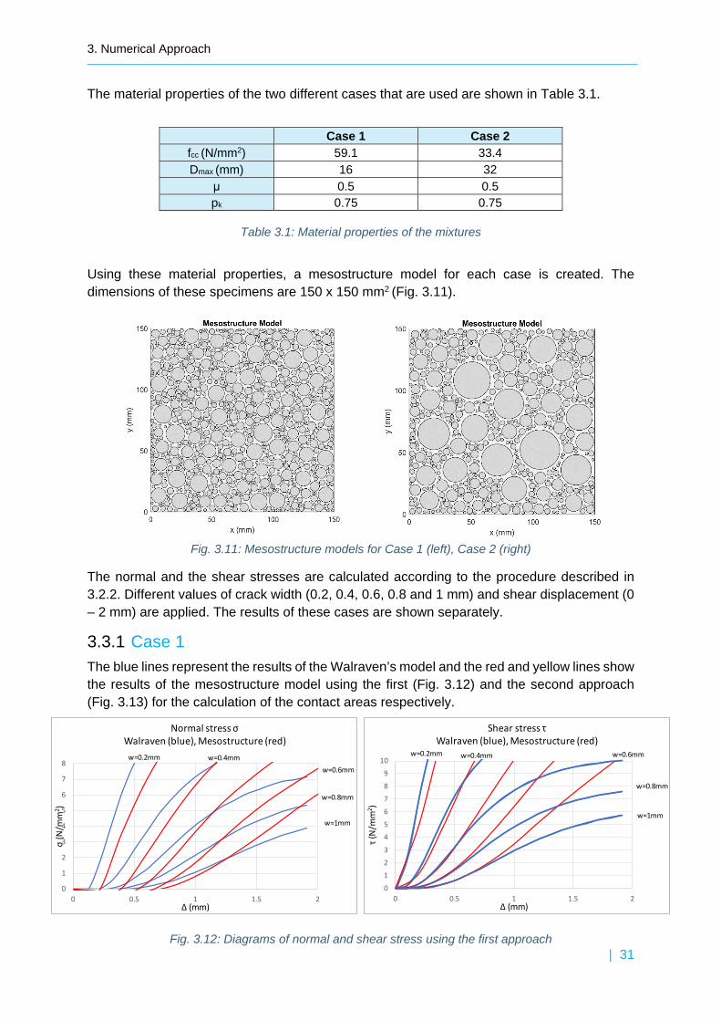
The material properties of the two different cases that are used are shown in Table 3.1.

Case 1 Case 2

fcc (N/mm2) 59.1 33.4 Dmax (mm) 16 32

μ 0.5 0.5 pk 0.75 0.75

Table 3.1: Material properties of the mixtures

Using these material properties, a mesostructure model for each case is created. The dimensions of these specimens are 150 x 150 mm2 (Fig. 3.11).

The normal and the shear stresses are calculated according to the procedure described in 3.2.2. Different values of crack width (0.2, 0.4, 0.6, 0.8 and 1 mm) and shear displacement (0 – 2 mm) are applied. The results of these cases are shown separately.

3.3.1 Case 1 The blue lines represent the results of the Walraven’s model and the red and yellow lines show the results of the mesostructure model using the first (Fig. 3.12) and the second approach (Fig. 3.13) for the calculation of the contact areas respectively.

Fig. 3.11: Mesostructure models for Case 1 (left), Case 2 (right)


| 32

Fig. 3.13: Diagrams of normal and shear stress using the second approach

0

1

2

3

4

5

6

0 0.5 1 1.5 2

σ (Ν

/mm

2 )

Δ (mm)

Normal stress σWalraven (blue), Mesostructure (red)

w=0.2mm w=0.4mm

w=0.6mm

w=0.8mm

w=1mm

0

1

2

3

4

5

6

7

8

0 0.5 1 1.5 2

τ (Ν

/mm

2 )

Δ (mm)

Shear stress τWalraven (blue), Mesostructure (red)

w=0.2mm w=0.4mm w=0.6mm

w=0.8mm

w=1mm

0

1

2

3

4

5

6

0 0.5 1 1.5 2

σ (Ν

/mm

2 )

Δ (mm)

Normal stress σWalraven (blue), Mesostructure (yellow)

w=0.2mm w=0.4mm

w=0.6mm

w=0.8mm

w=1mm

0

1

2

3

4

5

6

7

8

0 0.5 1 1.5 2

τ (Ν

/mm

2 )

Δ (mm)

Shear stress τWalraven (blue), Mesostructure (black)

w=0.2mm w=0.4mm w=0.6mm

w=0.8mm

w=1mm

0

1

2

3

4

5

6

7

8

0 0.5 1 1.5 2

σ (Ν

/mm

2 )

Δ (mm)

Normal stress σWalraven (blue), Mesostructure (yellow)

w=0.2mm w=0.4mm

w=0.6mm

w=0.8mm

w=1mm

0123456789

10

0 0.5 1 1.5 2

τ (Ν

/mm

2 )

Δ (mm)

Shear stress τWalraven (blue), Mesostructure (yellow)

w=0.2mm w=0.4mm w=0.6mm

w=0.8mm

w=1mm

3.3.2 Case 2 The same results are presented for the second case.

Fig. 3.15: Diagrams of normal and shear stress using the second approach

Fig. 3.14: Diagrams of normal and shear stress using the first approach


| 33

Generally, it becomes clear that the numerical results are in line with the analytical.

It is observed that the results of the shear stresses for the first approach and the results for the normal stresses of the second approach agree better with the Walraven’s model.

In the first approach the mesostructure model is less stiff than the analytical model for low shear displacements. For larger shear displacements the model becomes stiffer. On the other hand, the second approach predicts smaller stresses for crack widths smaller than 0.2 mm compared to Walraven’s, but this is not the case for larger crack widths.

3.4 Conclusions A new simplified numerical approach based on Walraven’s theory is presented in this chapter. In order to verify that this approach could be used, a comparison between them was deemed necessary. The most reasonable way to accomplish that was the numerical development of the crack structure just like the proposed by Walraven. The numerical mesoscale modelling was considered suitable for that purpose. Subsequently, the calculation of the stresses was done according to Walraven’s model. More specifically, two cases were analyzed for the validation of this new model.

Regarding the validation procedure, it can be concluded that the results of the model are reliable compared to the analytical. The first approach of the calculation of the contact areas seems that in general underestimates the results, while the second overestimates them. Nevertheless, the two approaches, even the simplified second one, give satisfactory results.

These small deviations are probably due to the fact that in Walraven’s model the crack structure is given by a statistical analysis, while in the mesostructure model a numerical calculation takes place. In addition, a 3D mesostructure model, instead of a 2D, is likely to give more accurate results, which will correspond to the real structure of the specimen.

Finally, this proposed method appears to be suitable to analyze specimens with different concrete mixtures and strengths with adequate accuracy. Also, the fundamental assumption for the plasticity of the material proved reliable and thus the rest of this research will be based on this numerical approach.


| 34

| 35

Fig. 4.2: Aggregate grading curve Fig. 4.1: Concrete compressive strength development for Cast 17 & 18

0

10

20

30

40

50

60

70

80

90

100

0 20 40 60 80 100 120 140 160

fc (M

Pa)

Age (Days)

Cast 18

Cast 17

4 Surface roughness measurements

An experimental program was carried out in order to investigate the influence of the roughness on the aggregate interlock, because there is a lack of surface roughness measurements in the existing research studies. The test setup and the material properties of the specimens will be presented followed by the procedure for the measurement of roughness.

4.1 Test Program

4.1.1 Specimens For the execution of the experiments 4 cubes, 3 cylinders and 1 beam were used. In particular, splitting tests were performed to the cubes and the cylinders. The beam was subjected to shear test loaded by a point load. The measurements of the kinematics of the beam were done with the use of LVDTs and Digital Image Correlation. The properties of the specimens will be referred separately.

4.1.1.1 Cubes

Tests were done for 4 cubes with size of 150 x 150 x 150 mm3 from 2 different casts. The casts were conducted on the same day (28-03-2018) and after several tests from these casts, the development of their compressive strength is depicted in Fig. 4.1. The tests took place on the 77th day from the cast, so the concrete compressive strength on this day is calculated as fc,cube = 82.5 MPa for the two casts. The mixture was also the same for the different casts. The aggregate distribution curve was obtained from the concrete supplier of Stevinlab and it is given in Fig. 4.2. The maximum aggregate size of the mixture was 22.4 mm.

4. Experimental Program

| 36

Fig. 4.4: Remaining part of the beam

4.1.1.2 Cylinders

The cylinders were actually cores drilled from the Nieuwklap bridge in the Netherlands. The average measured compressive strength of them was 84.5 MPa and their dimensions are shown in Table 4.1. The aggregates had maximum grain size of 32 mm. Τhis large size is justified by the fact that the bridge was constructed in 1941, when the aggregates were coarser.

Cylinder Diameter (mm) Height (mm) 1 95.6 96.8 2 95.7 99.3 3 95.7 98.1

Table 4.1: Dimensions of the cylinders

4.1.1.3 Beam

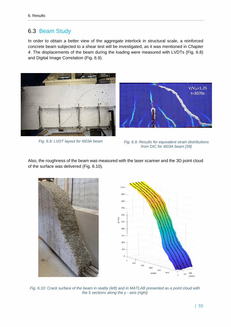
The beam, labeled as I603A, belongs to another project of the laboratory, so the following results were obtained from the relevant report [33]. The beam was casted together with the cubes in order to have the same strength development. The dimensions of the beam were H=1200mm, L=10000mm and W=300mm. The reinforcement was consisted of 4Ø25 plain bars without shear reinforcement. The compressive strength of the beam was found equal to 78.75 MPa and the concrete mixture was the same as the cubes. Initially, the beam presented a flexural failure at a load level of 299 kN and after the repositioning of the point load further from the support, it failed in shear at 5 kN.

Fig. 4.3: Remaining parts of cylinders (top) and cubes (bottom)


| 37

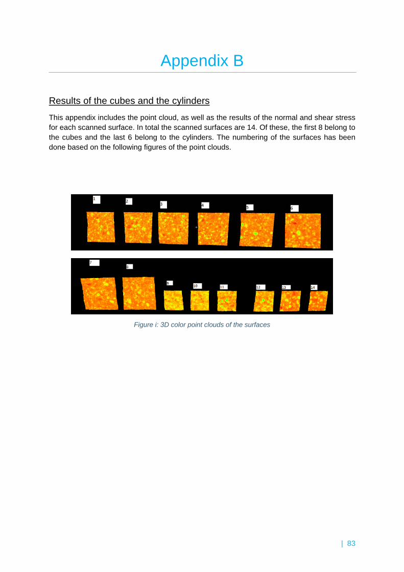
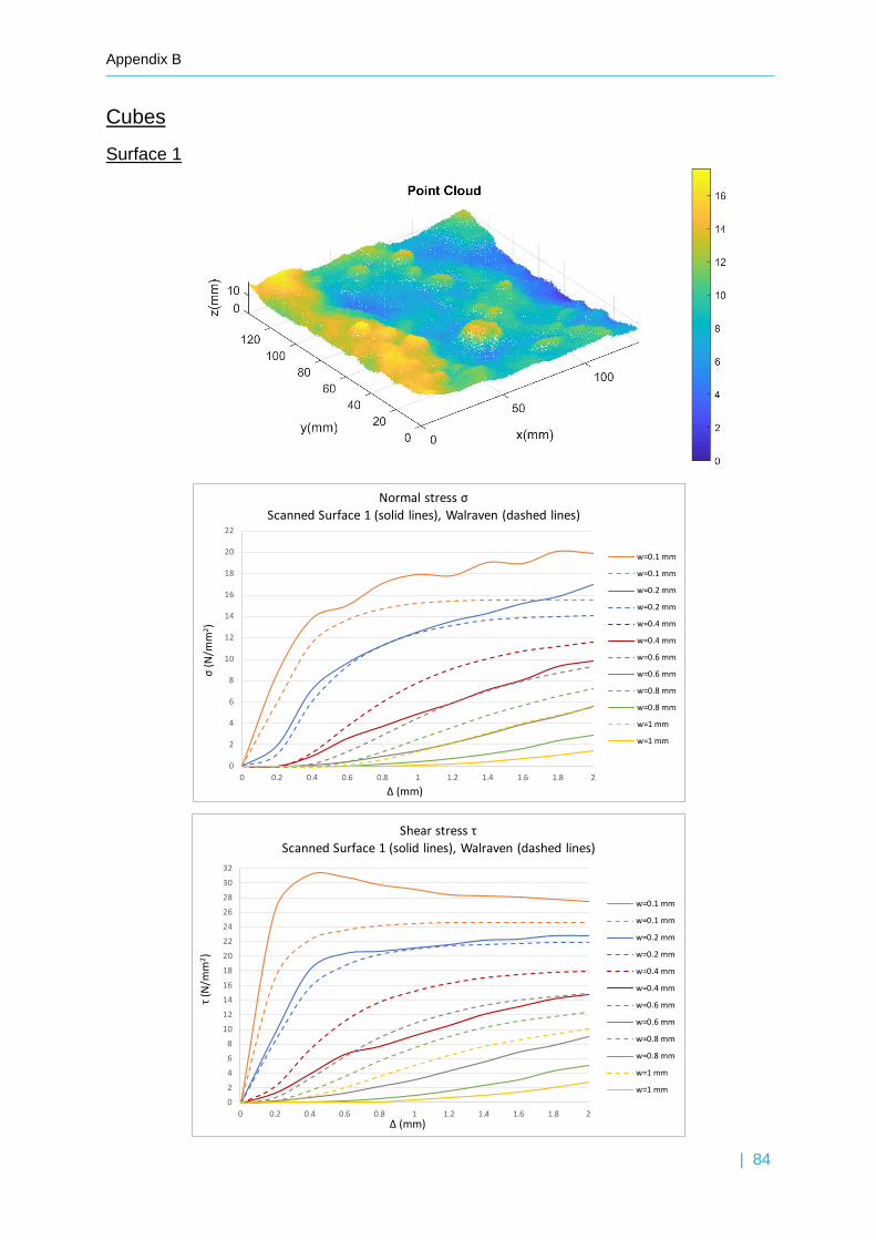
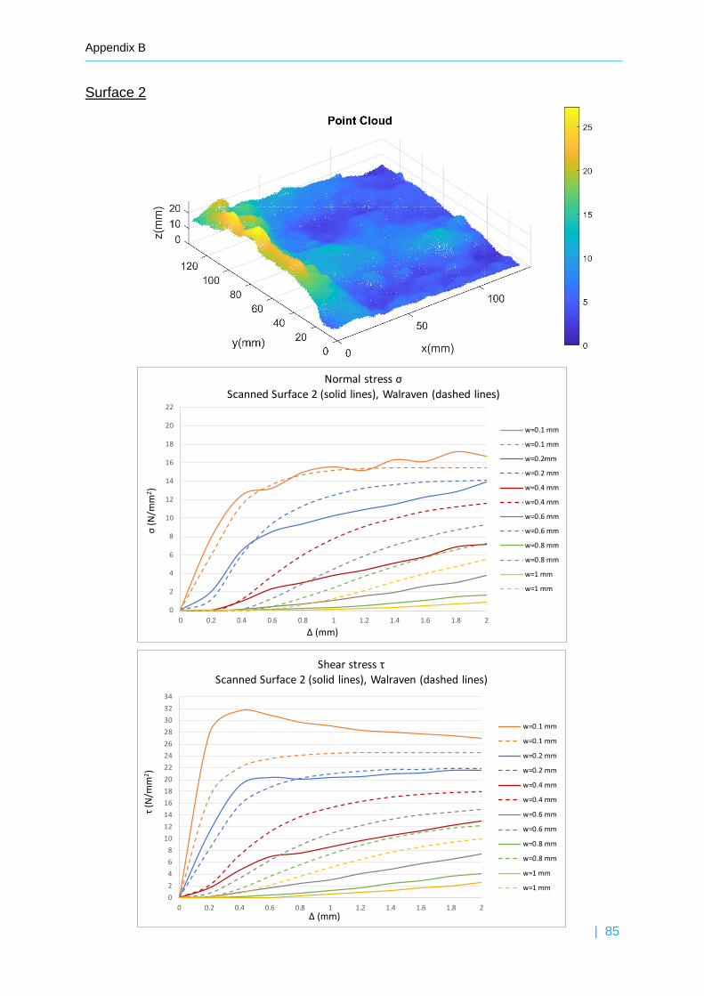
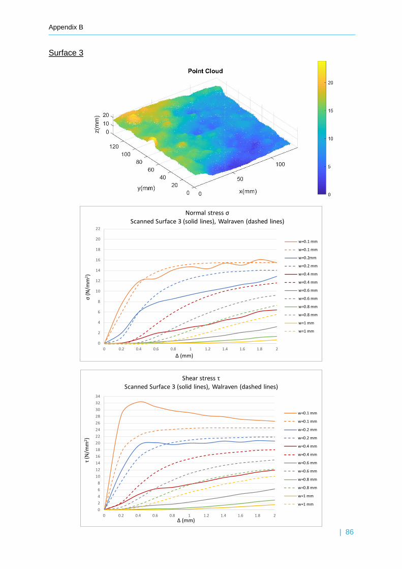
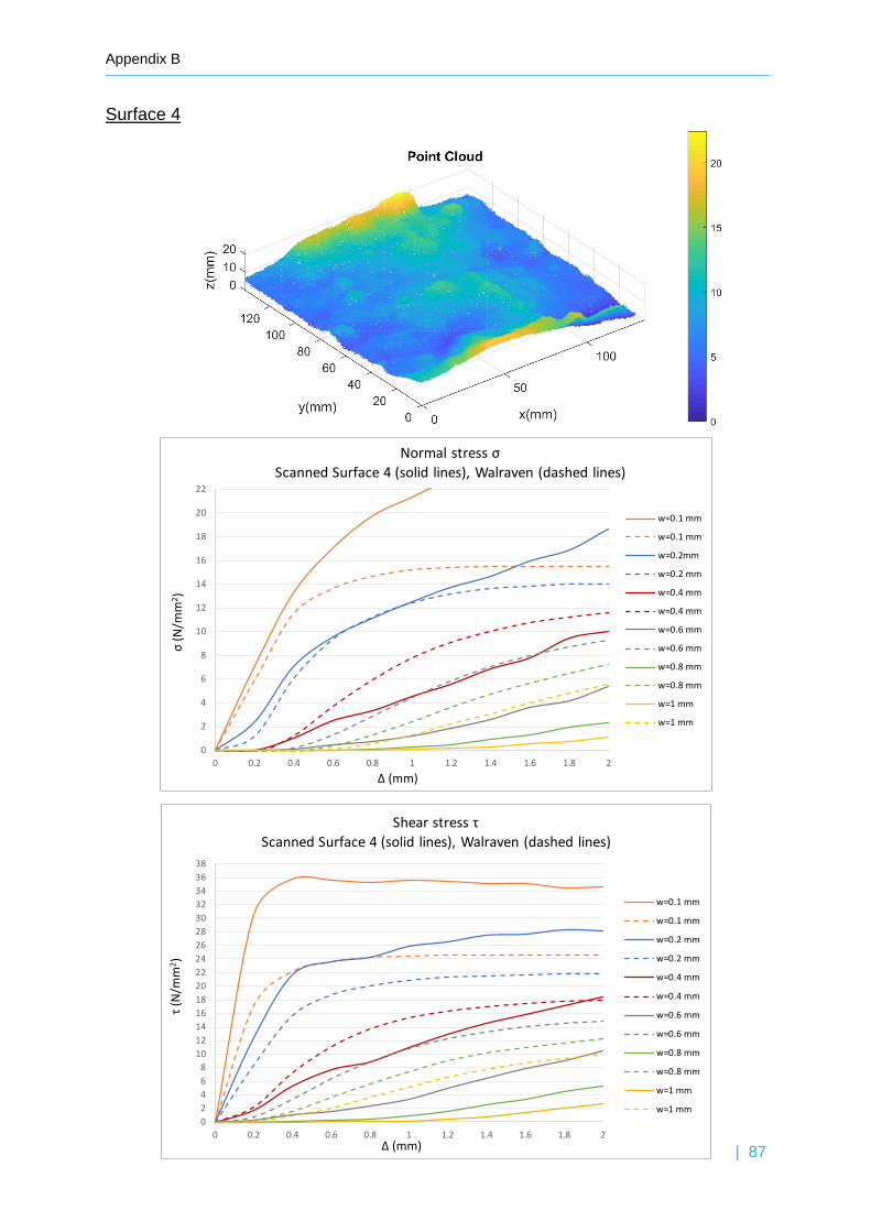
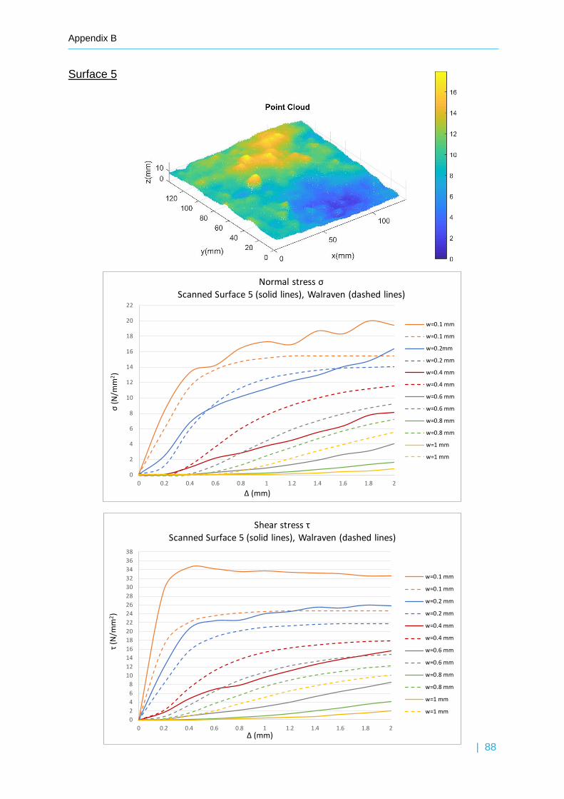
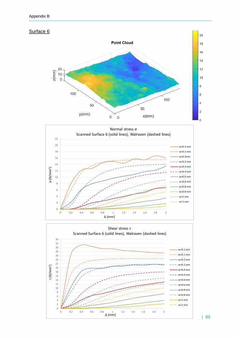
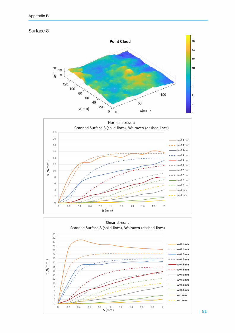
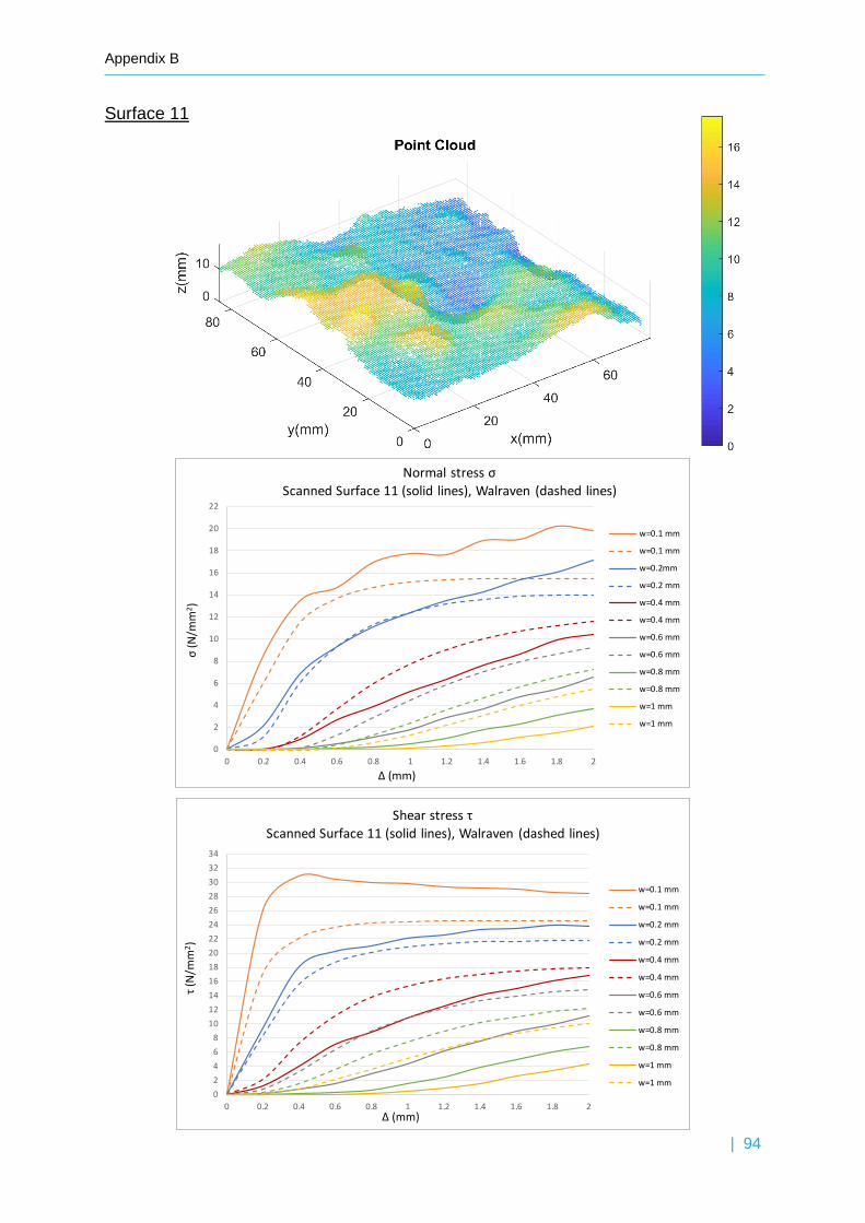
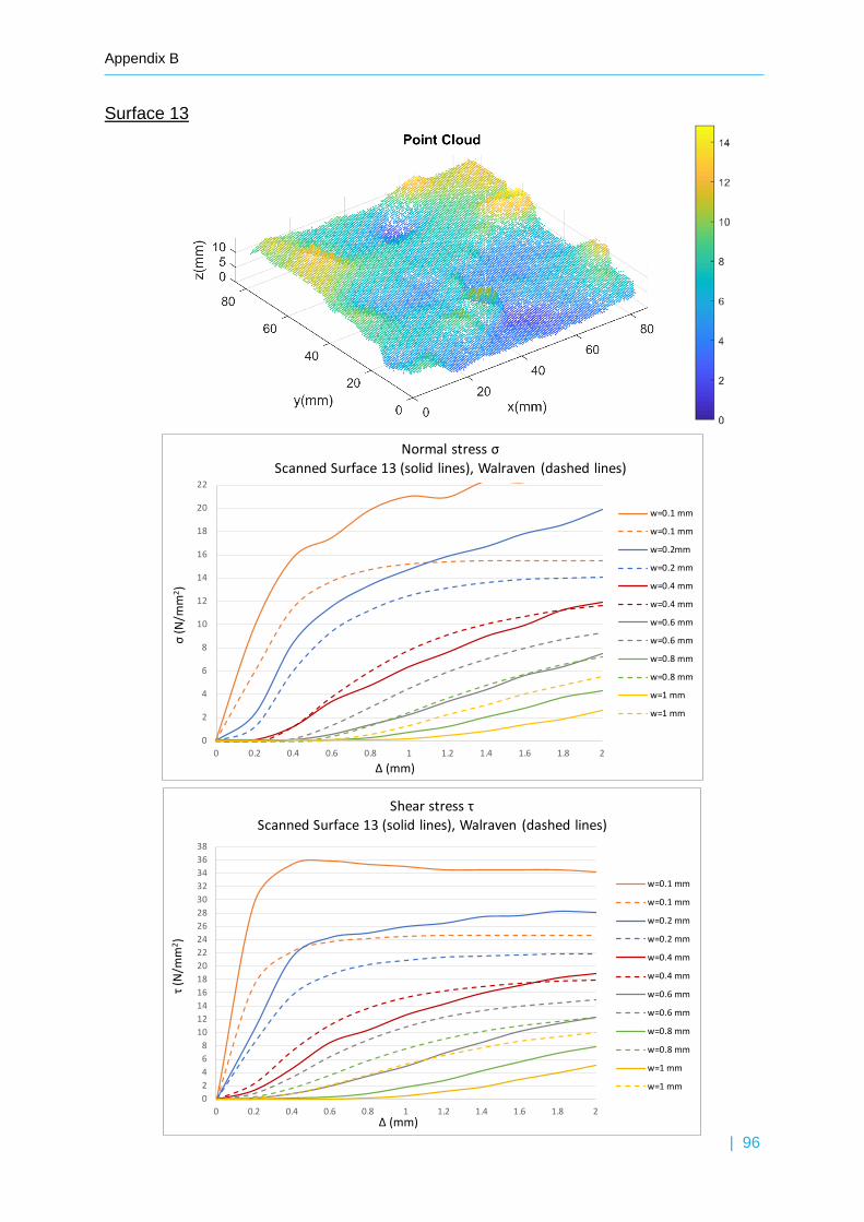
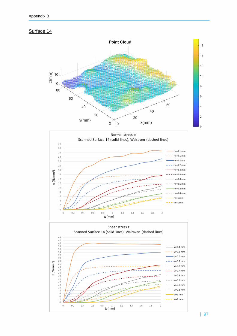
4.2 Roughness Measurements For the measurement of the roughness a laser scanner was necessary. For this purpose, a three-dimensional (3D) Leica scan station from the Gemeente of Rotterdam was used (Fig. 4.6). This high-resolution scanner is able to scan 1 million points per second with low range of noise. The remaining parts of the splitting tests and of the failure of the beam were scanned and a 3D point cloud with great accuracy and resolution of 0.1 mm was delivered for each cracked surface (Fig. 4.5).

Fig. 4.6: The laser scan station and the beam

Fig. 4.5: 3D color point clouds of the surfaces


| 38

| 39 Fig. 5.1: 3D point cloud of scanned surface 1 before (left) and after the rotation (right)

5 Crack Surface Geometry

After the measurements, a post-processing of the laser scanning data will follow in MATLAB software. The surfaces of the cubes and cylinders will be analyzed here.

The topography of the cracked concrete surfaces plays an important role in the aggregate interlock mechanism and generally in the estimation of the shear resistance. For this reason, it will be further investigated in this chapter. It can be described with various methods, but two of them will be analyzed in detail for the measured crack faces: the surface roughness index and the angle distribution of the surfaces.

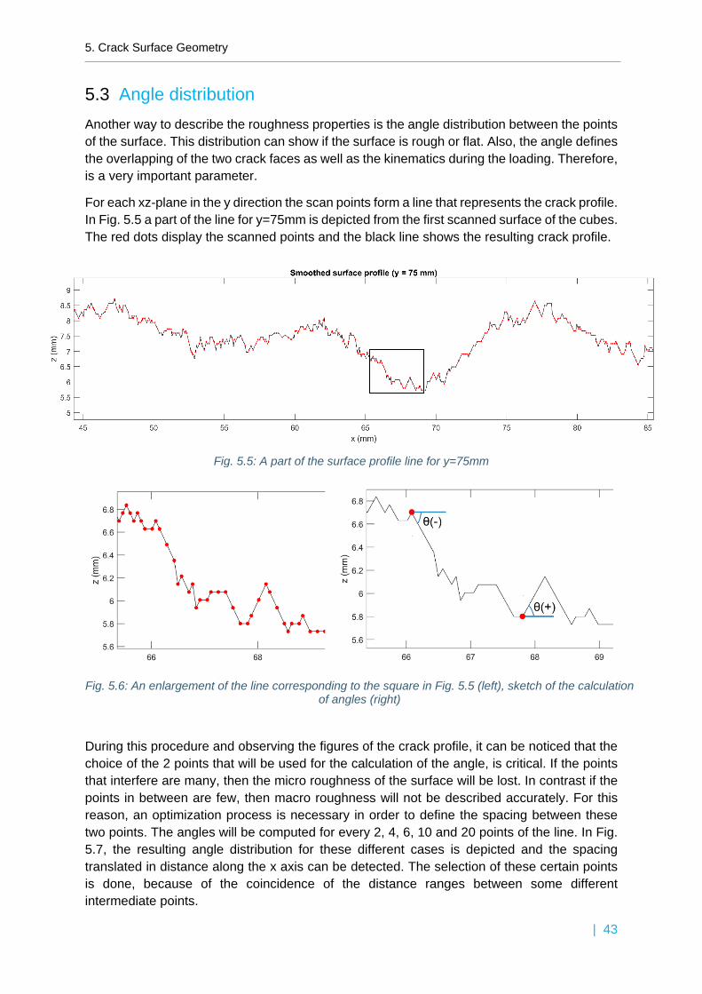
5.1 Post-processing of laser scanning data The raw data obtained from the laser scanning are represented as a set of points in 3D space. Before the point cloud can be used, should be rotated so that the surface roughness corresponds to variations in a particular direction. In this project this direction is selected to be the z axes (Fig. 5.1). The rotation of the point cloud is done with the help of CloudCompare, a 3D point cloud processing software. After the rotation of the point cloud, the filtering of the noisy data is necessary in order to correctly interpret the results. For this purpose, the used method is the moving average filtering, which smooths data by replacing each data point with the average of the neighboring data points defined within the span [34]. This method is considered accurate enough, because this project focuses on the height variations in an average aggregate size level and not in micro level. Also, due to the lack of time and the possibility for the repetition of the measurements the use of the information of the neighboring data points, according to this method, is a useful tool for the filtering. The span that is used consists of 5 points (Fig. 5.2). In Fig. 5.3, an example of a line extracted from the point cloud is depicted. The post-processed point clouds of all the surfaces are included in Appendix B.

5. Crack Surface Geometry

| 40

Fig. 5.2: Graphic representation of moving average with a span of five points

5.2 Surface Roughness Index There are many roughness quantification parameters but in this project the roughness index according to Perera and Mutsuyoshi is selected because their method of measurement was similar to the one that is applied during this research [35]. They also used fractured splitting test specimens and they measured them with a laser light confocal microscope. The roughness index was calculated according to the following formula:

𝑅𝑅𝑠𝑠 =∑𝐴𝐴𝑚𝑚∑𝐴𝐴

(5.1)

where 𝐴𝐴𝑚𝑚 is the fractured area and 𝐴𝐴 is the projected surface area (Fig. 5.4)

Fig. 5.3: Surface profile before (top) and after (bottom) the filtering


| 41

Fig. 5.4: Schematic view of roughness index

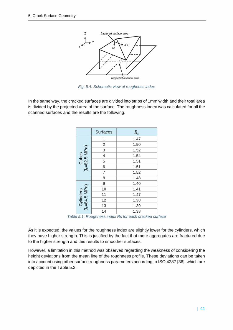
In the same way, the cracked surfaces are divided into strips of 1mm width and their total area is divided by the projected area of the surface. The roughness index was calculated for all the scanned surfaces and the results are the following.

Table 5.1: Roughness index Rs for each cracked surface

As it is expected, the values for the roughness index are slightly lower for the cylinders, which they have higher strength. This is justified by the fact that more aggregates are fractured due to the higher strength and this results to smoother surfaces.

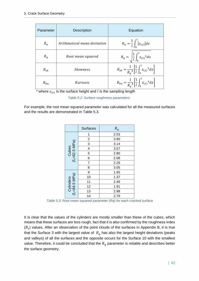
However, a limitation in this method was observed regarding the weakness of considering the height deviations from the mean line of the roughness profile. These deviations can be taken into account using other surface roughness parameters according to ISO 4287 [36], which are depicted in the Table 5.2.

Surfaces 𝑅𝑅𝑠𝑠

Cub

es

(f c=8

2.5

MPa

)

1 1.47 2 1.50 3 1.52 4 1.54 5 1.51 6 1.51 7 1.52 8 1.48

Cyl

inde

rs

(f c=8

4.5

MPa

) 9 1.40 10 1.41 11 1.47 12 1.38 13 1.39 14 1.38


| 42

Parameter Description Equation

𝑅𝑅𝑚𝑚 𝐴𝐴𝑎𝑎𝑎𝑎𝑡𝑡ℎ𝑚𝑚𝐹𝐹𝑡𝑡𝑎𝑎𝑐𝑐𝑎𝑎𝑚𝑚 𝑚𝑚𝐹𝐹𝑎𝑎𝑛𝑛 𝑑𝑑𝐹𝐹𝑣𝑣𝑎𝑎𝑎𝑎𝑡𝑡𝑎𝑎𝑐𝑐𝑛𝑛 𝑅𝑅𝑚𝑚 =1𝑚𝑚� �𝑧𝑧(𝑥𝑥)�𝑑𝑑𝐷𝐷𝑙𝑙

0

𝑅𝑅𝑞𝑞 𝑅𝑅𝑐𝑐𝑐𝑐𝑡𝑡 𝑚𝑚𝐹𝐹𝑎𝑎𝑛𝑛 𝑠𝑠𝑠𝑠𝑢𝑢𝑎𝑎𝑎𝑎𝐹𝐹𝑑𝑑 𝑅𝑅𝑞𝑞 = �1𝑚𝑚� 𝑧𝑧(𝑥𝑥)

2𝑑𝑑𝐷𝐷𝑙𝑙

0

𝑅𝑅𝑠𝑠𝑐𝑐 𝐴𝐴𝑘𝑘𝐹𝐹𝑤𝑤𝑛𝑛𝐹𝐹𝑠𝑠𝑠𝑠 𝑅𝑅𝑠𝑠𝑐𝑐 =1𝑅𝑅𝑞𝑞3

�1𝑚𝑚� 𝑧𝑧(𝑥𝑥)


0�

𝑅𝑅𝑐𝑐𝑝𝑝 𝐾𝐾𝑢𝑢𝑎𝑎𝑡𝑡𝑐𝑐𝑠𝑠𝑎𝑎𝑠𝑠 𝑅𝑅𝑐𝑐𝑝𝑝 =1𝑅𝑅𝑞𝑞4

�1𝑚𝑚� 𝑧𝑧(𝑥𝑥)


0�

* where 𝑧𝑧(𝑥𝑥) is the surface height and 𝑚𝑚 is the sampling length

For example, the root mean squared parameter was calculated for all the measured surfaces and the results are demonstrated in Table 5.3.

It is clear that the values of the cylinders are mostly smaller than these of the cubes, which means that these surfaces are less rough, fact that it is also confirmed by the roughness index (𝑅𝑅𝑠𝑠) values. After an observation of the point clouds of the surfaces in Appendix B, it is true that the Surface 3 with the largest value of 𝑅𝑅𝑞𝑞 has also the largest height deviations (peaks and valleys) of all the surfaces and the opposite occurs for the Surface 10 with the smallest value. Therefore, it could be concluded that the 𝑅𝑅𝑞𝑞 parameter is reliable and describes better the surface geometry.

Table 5.2: Surface roughness parameters

Surfaces 𝑅𝑅𝑞𝑞

Cub

es

(f c=8

2.5

MPa

)

1 2.53 2 3.90 3 3.14 4 3.57 5 2.80 6 2.08 7 2.29 8 3.05

Cyl

inde

rs

(f c=8

4.5

MPa

) 9 1.65 10 1.37 11 2.49 12 1.91 13 2.98 14 2.79

Table 5.3: Root mean squared parameter (Rq) for each cracked surface


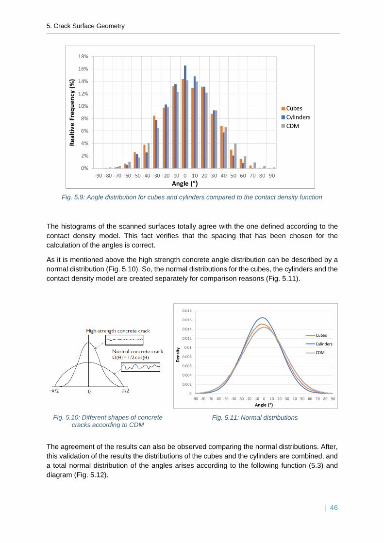
| 43

5.3 Angle distribution Another way to describe the roughness properties is the angle distribution between the points of the surface. This distribution can show if the surface is rough or flat. Also, the angle defines the overlapping of the two crack faces as well as the kinematics during the loading. Therefore, is a very important parameter.

For each xz-plane in the y direction the scan points form a line that represents the crack profile. In Fig. 5.5 a part of the line for y=75mm is depicted from the first scanned surface of the cubes. The red dots display the scanned points and the black line shows the resulting crack profile.

During this procedure and observing the figures of the crack profile, it can be noticed that the choice of the 2 points that will be used for the calculation of the angle, is critical. If the points that interfere are many, then the micro roughness of the surface will be lost. In contrast if the points in between are few, then macro roughness will not be described accurately. For this reason, an optimization process is necessary in order to define the spacing between these two points. The angles will be computed for every 2, 4, 6, 10 and 20 points of the line. In Fig. 5.7, the resulting angle distribution for these different cases is depicted and the spacing translated in distance along the x axis can be detected. The selection of these certain points is done, because of the coincidence of the distance ranges between some different intermediate points.

Fig. 5.5: A part of the surface profile line for y=75mm

Fig. 5.6: An enlargement of the line corresponding to the square in Fig. 5.5 (left), sketch of the calculation of angles (right)


| 44

More specifically, the histogram in Fig. 5.7 illustrates the relative frequency of the angles, as they are taken from 10 lines of the first measured surface of the specimens. The angles are divided into 19 intervals from -90° until 90°. It can be clearly observed that for each case, the angles are symmetrical distributed between the negative and the positive angle values.

Regarding the orange bar chart that represents the distance range of 0.1 - 0.3 mm, the bigger frequency of angles is in -40° and 50°. This means that the surface is quite rough, and this is not realistic because the macro roughness, which is flatter, is not taken into account. Also, for the chart of 4 points the percentages of the angles from -40° to 40° are high. On the other hand, the charts of angles for every 10 and 20 points result in smoother surfaces with inclinations of -10° to 10°. In this way the more inclined parts, that describe the micro roughness, are neglected.

Thus, the distribution of the angles for the dense spacing tends to be smaller around 0° and higher for the steeper inclinations and vice versa. The final choice is the calculation of the angle distribution for every 6 of the scanned points along a line. This implies that the surface profile is divided into smaller intervals of 0.5 - 0.7mm length and their inclinations are computed. In this case, there is a better distribution of the angles, which corresponds to the reality.

The angle distributions for all the scanned surfaces are determined separately and an average distribution for the cubes and the cylinders is obtained and is depicted in Fig. 5.8.

Fig. 5.7: The angle distribution for every case


| 45

0%

2%

4%

6%

8%

10%

12%

14%

16%

18%

-90 -80 -70 -60 -50 -40 -30 -20 -10 0 10 20 30 40 50 60 70 80 90

Real

tive

Freq

uenc

y (%

)

Angle (°)

CubesCylinders

It can be observed that the relative frequency around 0° is higher for the cylinders compared to the cubes. This means that the surface of the cylinders is slightly smoother. The same conclusion occurred from the calculation of the roughness index in 5.2. Moreover, the majority of the relative frequencies (over 90%) is concentrated around the region of -40° to 40°, which characterizes the flat part, and insignificant percentages are noticed in the most inclined parts. This observation verifies that the surfaces are constructed of high strength concrete.

According to Contact Density Model (CDM), the angle distribution is described better by a normal distribution due to the higher concertation of flat planes in high strength concrete [20]. Therefore, the contact density function, considering the fracture of the aggregates, is expressed by the following form of the truncated normal distribution:

𝛺𝛺(𝜃𝜃) = 56

exp �−21 �𝜃𝜃𝜋𝜋�2� (𝜃𝜃 𝑎𝑎𝑠𝑠 𝑎𝑎𝑎𝑎𝑑𝑑𝑎𝑎𝑎𝑎𝑛𝑛) (5.2)

Using this probability density function, a large number of angles (20000 values) in degrees are generated using MATLAB, and the histogram is created, which is compared with that of the cubes and the cylinders and the results are shown in Fig. 5.9.

Fig. 5.8: Angle distribution for cubes and cylinders


| 46

0%

2%

4%

6%

8%

10%

12%

14%

16%

18%

-90 -80 -70 -60 -50 -40 -30 -20 -10 0 10 20 30 40 50 60 70 80 90

Real

tive

Freq

uenc

y (%

)

Angle (°)

CubesCylindersCDM

0

0.002

0.004

0.006

0.008

0.01

0.012

0.014

0.016

0.018

-90 -80 -70 -60 -50 -40 -30 -20 -10 0 10 20 30 40 50 60 70 80 90

Dens

ity

Angle (°)

Cubes

Cylinders

CDM

The histograms of the scanned surfaces totally agree with the one defined according to the contact density model. This fact verifies that the spacing that has been chosen for the calculation of the angles is correct.

As it is mentioned above the high strength concrete angle distribution can be described by a normal distribution (Fig. 5.10). So, the normal distributions for the cubes, the cylinders and the contact density model are created separately for comparison reasons (Fig. 5.11).

The agreement of the results can also be observed comparing the normal distributions. After, this validation of the results the distributions of the cubes and the cylinders are combined, and a total normal distribution of the angles arises according to the following function (5.3) and diagram (Fig. 5.12).

Fig. 5.9: Angle distribution for cubes and cylinders compared to the contact density function

Fig. 5.10: Different shapes of concrete cracks according to CDM

Fig. 5.11: Normal distributions


| 47

0

0.002

0.004

0.006

0.008

0.01

0.012

0.014

0.016

0.018

-90 -80 -70 -60 -50 -40 -30 -20 -10 0 10 20 30 40 50 60 70 80 90

Den

sity

Angle (°)

𝛺𝛺(𝜃𝜃) = 2129

exp �− 𝜃𝜃2

1324� (𝜃𝜃 𝑎𝑎𝑠𝑠 𝑑𝑑𝐹𝐹𝐿𝐿𝑎𝑎𝐹𝐹𝐹𝐹𝑠𝑠) (5.3)

5.4 Conclusions The crack surface geometry, which affects significantly the aggregate interlock mechanism, is investigated in this chapter. In order to have accurate and reliable results from the scanned surfaces, the noise from the raw laser data should be removed. Therefore, the rotation and the de-noising of the point cloud for each surface was done.

Two ways for describing the roughness properties of the surface were considered representative for this project. The roughness index and the angle distribution of the surface are important parameters that can be used to compare different crack profiles.

At first, the roughness index was proved a simple and reliable way of describing the surface. However, a weakness of considering the height deviations from the mean line was observed and alternative parameters were proposed with an application for one of them.

The angle distribution of the surfaces defines the amount of contact areas and the displacements during the loading. The statistical distribution of them showed that the choice of the spacing between the points that define the angle, is critical. It is concluded that the finer scan recognizes more inclined parts than a coarser one and results in a normal distribution with higher percentages for the steeper inclinations. In that case the macro roughness is neglected. The opposite happens for coarser laser scan data. Therefore, the angle distribution may not be representative of the real surface as it is already mentioned in the literature of Contact Density Model [20]. However, it can be useful for qualitative understanding and comparison between surfaces if the same spacing is kept for the calculation of the angles. For that reason, different spacings were compared and the final choice was the interval length of 0.5 - 0.7mm, which gave logical results that correspond to the reality. This choice validated that it was in line with the CDM and a new probability density function was proposed based on the results of the scanned surfaces.

Fig. 5.12: Total angle distribution


| 48

| 49

Fig. 6.1: Cracking representation of the specimen applying 1mm crack width (w) and 2mm shear displacement (Δ)

6 Aggregate interlock based on measured

crack surfaces

After the validation of the proposed numerical approach for the calculation of the aggregate interlock in Chapter 3, the application of this model will be done in this chapter for the scanned surfaces. At first, this model will be adopted for these surfaces, but the calculation process will be reserved. So, a numerical model, based on a MATLAB code, that will calculate the aggregate interlock using the data of the scanned surfaces, will be proposed.

Subsequently, the fracture of the aggregates will be investigated and a new factor for the aggregate interlock, considering the fracture of the aggregates will be proposed.

The results for the measured beam will be presented afterwards, followed by an investigation about the influence of the simplification of the crack profile. Finally, a master curve will be proposed based on the results of the measured cracked surface of the beam that will be able to predict directly the stresses for beams with the same material properties.

6.1 Adoption of the numerical approach to scanned surfaces In this case with the scanned surfaces, the structure of the surfaces is given as an input with the form of a point cloud, instead of the creation of a mesostructure model like in Chapter 3. After this point, the code continues as it was described.

The point cloud is introduced in MATLAB (Fig. 5.1) and is divided into strips of 1mm width. Each strip represents a crack profile (Fig. 5.3). After the de-noising, the strip is duplicated and is shifted for a certain normal (w) and shear displacement (Δ). In this way, the behavior of the cracking during the loading is represented (Fig. 6.1).

w

Δ

6. Results

| 50

The contact areas followed by the stresses are calculated for all the strips and then the average value for the normal (σ) and shear (τ) stress is determined, according to Walraven’s model. The MATLAB code is attached in Appendix A.

6.2 Fracture of the aggregates As it was already mentioned, in normal strength concrete (until 50 MPa), the cement matrix is less strong than the aggregates and as a result, the crack propagates around the aggregates. The basic assumption in Walraven’s model is that the aggregates do not fracture. In high strength concrete this is not the case. The aggregates fracture, because they have lower strength than the cement matrix. Due to this fact, the fractured aggregates do not contribute to the aggregate interlock resistance and a reduction factor should be considered.

According to Walraven [13], this reduction factor is regarded as a material parameter known as fracture index 𝐶𝐶𝑣𝑣, which reduces the contact areas. It takes values from 0 to 1 and it can be estimated by shear tests. The relations for the calculation of stresses become:

𝜎𝜎 = 𝐶𝐶𝑣𝑣 ∙ 𝜎𝜎𝑝𝑝𝑝𝑝 ∙ ��̅�𝐴𝑥𝑥 − 𝜇𝜇 ∙ �̅�𝐴𝑦𝑦� 𝜏𝜏 = 𝐶𝐶𝑣𝑣 ∙ 𝜎𝜎𝑝𝑝𝑝𝑝 ∙ (�̅�𝐴𝑦𝑦 + 𝜇𝜇 ∙ �̅�𝐴𝑥𝑥) (6.1)

Walraven and Stroband [37] found from experiments in high strength concrete (110 MPa) a reduction factor 𝐶𝐶𝑣𝑣 equal to 0.35, which means that 75% of the aggregates fracture.

Yang [14] using a database of shear test results, improved this reduction factor, introducing the significant parameter of concrete strength.

𝑅𝑅𝑚𝑚𝑚𝑚 = 0.85��7.2

𝐶𝐶𝑐𝑐 − 40 + 1�2

− 1 + 0.34 (6.2)

In this project, experiments were done for high strength concrete (82.5 & 84.5 MPa) and the results for the aggregate interlock stresses are given according to the numerical approach that is described in 6.1. This approach takes into account the fracture of the aggregates, as long as the stresses are estimated based on the scanned surfaces that already contain fractured aggregates. In order to quantify the influence of the aggregate fracture, the results of the

Fig. 6.2: An enlargement of the crack corresponding to the square in Fig. 6.1

6. Results

| 51

Fig. 6.3: Diagrams of normal (top) and shear (bottom) stresses for the scanned surface 1 and Walraven’s model (5-point moving average)

0

2

4

6

8

10

12

14

16

18

20

22

0 0.2 0.4 0.6 0.8 1 1.2 1.4 1.6 1.8 2

σ (Ν

/mm

2 )

Δ (mm)

Normal stress σScanned Surface 1 (solid lines), Walraven (dashed lines)

w=0.1 mm

w=0.1 mm

w=0.2 mm

w=0.2 mm

w=0.4 mm

w=0.4 mm

w=0.6 mm

w=0.6 mm

w=0.8 mm

w=0.8 mm

w=1 mm

w=1 mm

scanned surfaces are compared with Walraven’s model. This is performed by inserting the material properties of the cube in the model (concrete strength fc and maximum diameter of the aggregates Dmax).

In Fig. 6.3 these results are presented for various crack widths w (0.1, 0.2, 0.4, 0.6, 1 mm) and shear displacements Δ (0 - 2 mm). The dashed lines represent the results of Walraven’s model and the solid lines these of the first scanned surface (cube). Similar diagrams are observed for all the scanned surfaces and can be found in Appendix B.

0

2

4

6

8

10

12

14

16

18

20

22

24

26

28

30

32

0 0.2 0.4 0.6 0.8 1 1.2 1.4 1.6 1.8 2

τ (Ν

/mm

2 )

Δ (mm)

Shear stress τScanned Surface 1 (solid lines), Walraven (dashed lines)

w=0.1 mm

w=0.1 mm

w=0.2 mm

w=0.2 mm

w=0.4 mm

w=0.4 mm

w=0.6 mm

w=0.6 mm

w=0.8 mm

w=0.8 mm

w=1 mm

w=1 mm

6. Results

| 52

Fig. 6.4: Diagrams of normal (top) and shear (bottom) stresses for the scanned surface 1 and Walraven’s model (13-point moving average)

0

2

4

6

8

10

12

14

16

18

20

22

24

26

0 0.2 0.4 0.6 0.8 1 1.2 1.4 1.6 1.8 2

τ (Ν

/mm

2 )

Δ (mm)


w=0.1 mm

w=0.1 mm

w=0.2 mm

w=0.2 mm

w=0.4 mm

w=0.4 mm

w=0.6 mm

w=0.6 mm

w=0.8 mm

w=0.8 mm

w=1 mm

w=1 mm

0

2

4

6

8

10

12

14

16

18

20

22

0 0.2 0.4 0.6 0.8 1 1.2 1.4 1.6 1.8 2

σ (Ν

/mm

2 )

Δ (mm)


w=0.1 mm

w=0.1 mm

w=0.2mm

w=0.2 mm

w=0.4 mm

w=0.4 mm

w=0.6 mm

w=0.6 mm

w=0.8 mm

w=0.8 mm

w=1 mm

w=1 mm

Generally, the diagrams follow the same pattern, fact that verifies, for one more time, that the numerical approach is reliable. It is clear that, until the crack width of 0.2 mm, the numerical approach overestimates the normal and the shear stresses. On the other hand, for larger crack widths the results are underestimated compared to Walraven’s model. This overestimation in small crack widths is probably explained by the fact that the selected method for filtering the data is not able to remove all the noisy data and the surfaces have micro-irregularities that do not correspond to the real surfaces and cause larger contact areas. In fact, these micro-irregularities exist at the early stages of the crack opening, but due to the lower strength of mortar break quickly and easily. As the crack width becomes larger the deviation from Walraven’s model increases. This means that the fracture of the aggregates influences significantly the results in larger crack widths and there is no more contribution of aggregate interlock.

In order to confirm the hypothesis for the overestimation in smaller crack widths, an example of using the method of moving average between 13 points, instead of 5, is used and the results are the following (Fig. 6.4).

6. Results

| 53

y = -0.7891x + 0.9213R² = 0.5662

-0.1

0.0

0.1

0.2

0.3

0.4

0.5

0.6

0.7

0.8

0.9

0.00 0.20 0.40 0.60 0.80 1.00

σ sa

cn/σ

Wal

rave

n

w (mm)

y = -0.8616x + 0.9454R² = 0.7045

0

0.1

0.2

0.3

0.4

0.5

0.6

0.7

0.8

0.9

0.00 0.20 0.40 0.60 0.80 1.00

τ sac

n/τ

Wal

rave

n

w (mm)

Actually, a comparison between Fig. 6.3 and Fig. 6.4 shows that the results for larger crack widths are not significantly affected, but for the smaller ones, until the crack width of 0.2 mm, the decrease is noteworthy. This means that the resulting smoother surface after the filtering of 13-point moving average, does not cause micro-irregularities that affect the results. The stresses are underestimated compared to Walraven’s, fact that corresponds to reality due to the fracture of the aggregates. However, in the diagram (Fig. 6.4 - top) of the normal stresses for w < 0.2 mm it is clear that the stresses are decreased for small values of shear displacement (Δ), but after a certain point they are overestimated just like in Fig. 6.3. This indicates that the normal stress for large shear displacements is not affected by the smoothing of the surface.

The height deviations of these spikes are describing irregularities in the cement paste and their sizes are much smaller than the aggregate sizes, which is the subject of this research. For this reason, the results for crack widths smaller than 0.2 mm could be neglected.

After these observations, it is obvious that the influence of the aggregate fracture depends on the crack width and should be taken into account. Therefore, the quantification of this influence occurs from the ratio of the results between the scanned surfaces and Walraven’s model, which is plotted against the crack width, for the abovementioned case (Fig. 6.5).

After the linear regression of the results, a fracture factor is generated that depends on the crack width. Combining the results of the stresses for all the surfaces the following diagrams occur and the linear regression equations are depicted (Fig. 6.6).

Fig. 6.5: Influence of aggregate fracture to normal (left) and shear stress (right) for scanned surface 1

6. Results

| 54

Fig. 6.6: Influence of aggregate fracture to normal (left) and shear stress (right) for all scanned surfaces

y = -0.7832x + 0.8827R² = 0.3145

-0.5

0.0

0.5

1.0

1.5

2.0

0.00 0.20 0.40 0.60 0.80 1.00

σ sa

cn/

σW

alra

ven

w (mm)

y = -0.8522x + 0.9472R² = 0.5015

0

0.2

0.4

0.6

0.8

1

1.2

1.4

0 0.2 0.4 0.6 0.8 1

τ sac

n/τ

Wal

rave

n

w (mm)

y = -0.8177x + 0.915R² = 0.3938

-0.4

-0.2

0.0

0.2

0.4

0.6

0.8

1.0

1.2

1.4

1.6

1.8

0.00 0.20 0.40 0.60 0.80 1.00

scan

/W

alra

ven

w (mm)

It can be observed that there are not large deviations between the different surfaces and normal and shear stresses. So, a common equation is possible to be generated. In Fig. 6.7 the combination of all the results is presented.

So, the proposed factor for the aggregate fracture can be expressed as:

𝑅𝑅𝑚𝑚𝑚𝑚 = −0.82 ∙ 𝑤𝑤 + 0.92 (6.3)

And the stress equations become:

𝜎𝜎 = 𝑅𝑅𝑎𝑎𝑎𝑎 ∙ 𝜎𝜎𝑝𝑝𝑝𝑝 ∙ ��̅�𝐴𝑥𝑥 − 𝜇𝜇 ∙ �̅�𝐴𝑦𝑦� 𝜏𝜏 = 𝑅𝑅𝑎𝑎𝑎𝑎 ∙ 𝜎𝜎𝑝𝑝𝑝𝑝 ∙ (�̅�𝐴𝑦𝑦 + 𝜇𝜇 ∙ �̅�𝐴𝑥𝑥) (6.4)

Fig. 6.7: Influence of aggregate fracture to normal and shear stress for all scanned surfaces

6. Results

| 55

6.3 Beam Study In order to obtain a better view of the aggregate interlock in structural scale, a reinforced concrete beam subjected to a shear test will be investigated, as it was mentioned in Chapter 4. The displacements of the beam during the loading were measured with LVDTs (Fig. 6.8) and Digital Image Correlation (Fig. 6.9).

Also, the roughness of the beam was measured with the laser scanner and the 3D point cloud of the surface was delivered (Fig. 6.10).

Fig. 6.9: Results for equivalent strain distributions from DIC for I603A beam [39]

Fig. 6.8: LVDT layout for I603A beam

Fig. 6.10: Crack surface of the beam in reality (left) and in MATLAB presented as a point cloud with the 5 sections along the y - axis (right)

6. Results

| 56

0

200

400

600

800

1000

1200

0 100 200 300 400 500 600 700 800 900 1000 1100 1200

z (m

m)

x (mm)

The crack profile is not uniform through the width of the beam (y - axis) and this fact can lead to different results for the aggregate interlock. For this reason, 5 strips of 1mm that represent a different crack profile are extracted every 50 mm along the width, as it is depicted in Fig. 6.10. The final stresses occur as the average value of these 5 sections.

The measured crack kinematics were given in segments along the height of the beam. For example, in Fig. 6.11 the beam is divided into 11 segments. The calculation of the stresses is done for each segment separately, according to the procedure that is described in 6.1. The segments are rotated in order to be their plane parallel to the x – axis and as a result the stresses are found in the local axes of each segment (Fig. 6.12).

Fig. 6.11: Segments along the height of the beam, where the kinematics are given (y = 150 mm)

2 3 4

5

6

7

1

8

9

11

10

Fig. 6.12: Rotation of segment 3 for the application of the kinematics

w

Δ

6. Results

| 57

0

50

100

150

200

250

300

350

0 1000 2000 3000 4000 5000 6000

Load

(kN

)

Time (s)

6.3.1 I603A Results For the calculation of the stresses of the beam the kinematics for 4 representative load levels are used. These load levels are shown with orange dots in Fig. 6.13 and their values in Table 6.1. The Vcr is the value of the shear force that is needed to open the critical inclined crack.

As an example, the evolution of the crack in time, for segment 5 is illustrated in Fig. 6.14. It is observed that at the first load level there is contact between the two cracked surfaces, which shows the contribution of the aggregate interlock. In the second load level, the contact is barely noticeable and finally it is lost due to the large displacements.

Load Levels V (kN) t (s)

1 234 2814 2 238 2982 3 299 4584 4 0 5134

Table 6.1: The 4 representative load levels

Fig. 6.13: Applied shear force for I603A beam vs time and the 4 representative load levels (orange dots)

Vcr

Fig. 6.14: Crack evolution in segment 5 for the 4 representative load levels

w= 0,79 mm & Δ=0.56 mm F=234 kN, t=2814 s

w= 2.19 mm & Δ=1.56mm F=238 kN, t=2982 s

w= 6.59 mm & Δ=5.37 mm F=299 kN, t=4584 s

w= 4.93 mm & Δ=3.23 mm F=0 kN, t=5134 s

6. Results

| 58

0

100

200

300

400

500

600

2800 3300 3800 4300 4800 5300

Forc

e (k

N)

t (s)

After the application of the measured kinematics and the calculation of the stresses, the aggregate interlock force is estimated, and the results are shown in Fig. 6.15. A sudden decay is observed after the first load level, where Vcr is reached. This loss of aggregate interlock leads to the failure of structure at t = 5134s.

6.3.2 Influence of the segments’ length in crack profile In many shear models, simplifications of the crack profile are used in order to simplify the calculation procedure and diminish its duration. For example, in CSD theory [14] the crack is simplified by two straight lines (Fig. 6.16). The main branch of the crack is assumed as a straight line at 90°. The secondary branch has a smaller inclination and is directed to the loading point.

In this project the real profile crack is used, but divided into a certain number of segments. This process arises interesting questions for an additional study. If the segments are many, then their lengths will be small, and the macro roughness (i.e. the curvature) of the crack profile may be neglected. On the other hand, the division into very few segments may be an over-simplification that affects the results. These assumptions will be examined further below.

The crack profile is divided into 11 (Fig. 6.11), 5, 3 and 2 segments (Fig. 6.17) for the calculation of the aggregate interlock stresses. Also, there is a case that the entire crack profile is examined as a segment.

Fig. 6.15: Aggregate interlock force for the 4 representative load levels

Fig. 6.16: Crack profile simplification based on CSDT [14]

6. Results

| 59

0

200

400

600

800

1000

1200

0 100 200 300 400 500 600 700 800 900 1000 1100 1200

z (m

m)

x (mm)

5 segments

0

200

400

600

800

1000

1200

0 200 400 600 800 1000 1200

z (m

m)

x (mm)

3 segments

0

200

400

600

800

1000

1200

0 200 400 600 800 1000 1200

z (m

m)

x (mm)

2 segments

For every case, shear displacements until 2 mm are applied for certain values of crack width (0.2, 0.4, 0.6, 0.8 & 1) and the aggregate interlock stresses are computed for each segment. Then, the average value of all the segments is found for the normal and shear stress separately. These results are presented in the following diagrams (Fig. 6.18). The blue line represents the results of the case of the whole profile as 1 segment, the green line the 2 segments, the orange line the 3 segments, the yellow line the 5 segments and the grey line the 11 segments.

Fig. 6.17: Division of the crack profile into 5, 3 & 2 segments (y = 150 mm)

1 2

3

4

5

1

1

2

2

3

6. Results

| 60

Fig. 6.18: Diagrams of normal and shear stresses for all the cases of different division of the crack profile

0

5

10

15

20

25

30

0 0.5 1 1.5 2

σ (Ν

/mm

2 )

Δ (mm)

Normal stress (w=0.2mm)

1

2

3

5

11

0

5

10

15

20

25

0 0.5 1 1.5 2

σ (Ν

/mm

2 )

Δ (mm)

Normal stress (w=0.4 mm)

1

2

3

5

11

0

2

4

6

8

10

12

14

16

18

0 0.5 1 1.5 2

σ (Ν

/mm

2 )

Δ (mm)


1

2

3

5

11

0

2

4

6

8

10

12

14

0 0.5 1 1.5 2

σ (Ν

/ mm

2 )

Δ (mm)


1

2

3

5

11

0

2

4

6

8

0 0.5 1 1.5 2

σ (Ν

/mm

2 )

Δ (mm)

Normal stress (w=1 mm)

1

2

3

5

11

0

5

10

15

20

25

30

35

40

45

0 0.5 1 1.5 2

τ (N

/mm

2 )

Δ (mm)

Shear stress (w=0.2 mm)

1

2

3

5

11

0

5

10

15

20

25

30

35

40

0 0.5 1 1.5 2τ (

N/m

m2 )

Δ (mm)


1

2

3

5

11

0

5

10

15

20

25

30

0 0.5 1 1.5 2

τ (N

/mm

2 )

Δ (mm)


1

2

3

5

11

0

5

10

15

20

25

0 0.5 1 1.5 2

τ (N

/mm

2 )

Δ (mm)


1

2

3

5

11

02468

101214161820

0 0.5 1 1.5 2

τ (N

/mm

2 )

Δ (mm)

Shear stress (w=1 mm)

1

2

3

5

11

6. Results

| 61

0

2

4

6

8

10

12

14

16

18

20

22

0 0.2 0.4 0.6 0.8 1 1.2 1.4 1.6 1.8 2

σ (Ν

/mm

2 )

Δ (mm)

Normal stress σI603A (solid lines), Walraven (dashed lines)

w=0.2mm

w=0.2mm

w=0.4mm

w=0.4mm

w=0.6mm

w=0.6mm

w=0.8mm

w=0.8mm

w=1mm

w=1mm

Fig. 6.19: Master curve of normal stress based on the surface measurements of I603A beam and Walraven’s model

It is obvious that the results of the beam divided into 2, 3, 5 and 11 segments are almost identical. On the other hand, there is a significant overestimation in the results of the whole crack profile compared to the other cases. This means that including the curvature of the profile, larger contact areas are formed, which produce larger contact stresses.

Consequently, the 2 segments of the crack profile that are implemented in the CSDT are adequate and provide reliable results. Also, the use of the two segments saves valuable computational time. Just like in CSDT the division of the segments should be done in that point that the inclination changes. This happens at the top part of the beam, where the inclination is small. In this case of the 2 segments the inclination of the secondary branch is equal to 22°. The main branch has an angle of 52°. Therefore, the assumption of the angle of 90° in CSDT should be changed.

6.3.3 Master curve After the investigation about the simplification of the crack profile and the conclusion that there are no deviations between the results of the stresses for the different cases (except of the case for 1 segment), a general curve can be generated based on I603A beam measured surface. This master curve will be applicable for beams with concrete strength around 80 MPa, maximum aggregate diameter of 22.4mm and for simplification of the profile until 2 segments. The only requirement for the calculation of stresses will be the knowledge of the kinematics for the different segments of the beam.

In Fig. 6.19 & Fig. 6.20 these master curves are presented for various crack widths w (0.2, 0.4, 0.6, 1 mm) and shear displacements Δ (0 - 2 mm). The solid lines represent the results based on the surface measurements of the scanned beam (I603A) and the dashed lines the equivalent results from Walraven’s model.

6. Results

| 62

0

2

4

6

8

10

12

14

16

18

20

22

24

26

0 0.2 0.4 0.6 0.8 1 1.2 1.4 1.6 1.8 2

τ(N

/mm

2 )

Δ (mm)

Shear stress τI603A (solid lines), Walraven (dashed lines)

w=0.2mm

w=0.2mm

w=0.4mm

w=0.4mm

w=0.6mm

w=0.6mm

w=0.8mm

w=0.8mm

w=1mm

w=1mm

Fig. 6.20: Master curves of shear stress based on the surface measurements of I603A beam and Walraven’s model

Fig. 6.21 Normal and shear displacements for H401A at the moment that V=Vcr

Again, an overestimation of the results, compared to Walraven’s, is observed until the 0.2mm crack width, which is explained by the intense micro roughness of the surface that causes larger contact areas than the real ones. However, after this crack width there is an underestimation, as it is expected due to the fracture of the aggregates.

An application of these master curves will follow for a different beam, labeled as H401A, that belongs to the same project of the laboratory. The measured kinematics for this beam are shown in Fig. 6.21.

Using the kinematics of the major crack, the normal and the shear stresses for every segment are found from the abovementioned master curves and an average value is calculated between the segments of the beam. From the comparison of these results with these that are estimated based on analytical model of Walraven, occurs that the normal stress from the master curve is smaller by 41% and the shear stress by 48% than the Walraven’s estimations. This can be observed clearly in Fig. 6.22, where the results of the shear transfer mechanisms are depicted with area charts separately and the applied shear force is represented by a red line.

6. Results

| 63

Fig. 6.22: Contribution of aggregate interlock force for H401A vs. time according to Walraven’s model (left) and according to the proposed master curves (right)

The aggregate interlock contribution in the shear force is bigger according to Walraven’s model (left), than the estimated by the proposed master curves (right). This result is expected, because the Walraven’s model does not take into account the fracture of the aggregates in HSC and as a result overestimates the shear forces.

6.4 Conclusions The results of the numerical approach using the measurements of the cracked surfaces are presented in this chapter, after a short description of the relevant MATLAB code. Using the results of the measured cracked surfaces from the cubes and the cylinders, the fracture of the aggregates is investigated, which occurs in HSC and is not considered in the existing models about the aggregate interlock. It is observed that the deviation between the numerical approach and Walraven’s model, which is due to the fracture of the aggregates, depends on the crack width. Therefore, this factor, that is proposed to be implemented into Walraven’s model, is dependent of the crack width and extends his model to high strength concrete.

Nevertheless, it is noticed that the stresses are overestimated for smaller crack widths (w ≤ 0.2 mm) and it is found that the reason of this fact is the presence of noisy data that make the surface rougher and cause larger stresses especially at small displacements. Due to the slight sizes of these spikes, that are negligible compared to the aggregate sizes, the results for crack widths smaller than 0.2 mm can be ignored in this research.

Regarding the results of the beam, is concluded that the aggregate interlock contributes significantly to the shear capacity, since its loss results in the failure of the beam. Taking motivation from the existing models, a study about the simplification of the crack profile is carried out, demonstrating that the simplification until 2 segments along the height of the profile is acceptable. Moreover, two modifications are proposed for the CSDT regarding the two abovementioned issues.

6. Results

| 64

Finally, a master curve is proposed for the estimation of the aggregate interlock stresses for beams without shear reinforcement and strength around to 80 MPa. Knowing the normal and the shear displacements for the segments of the beam, the stresses can be found easily.

| 65

7 Conclusions & Recommendations

This thesis makes an effort to fill the knowledge gap of estimating the aggregate interlock contribution in case of high strength concrete, because the existing models are suitable for normal strength concrete and at the same time the use of high strength concrete is becoming widespread. For this reason, a new approach and ways of improving the existing models are proposed using laser scanned surfaces and developing MATLAB codes.

7.1 Conclusions After a thorough study and engagement with the subject of this research the following conclusions can be drawn:

The thesis suggests the use of the plasticity model proposed by Walraven directly on scanned crack surface. In order to validate this approach, a hypothetic randomly distributed circular aggregate distribution was generated and used to compare Walraven’s theoretical model. The comparison demonstrated that the approach gives realistic estimations.

The laser scanning delivers a 3D point cloud that represents the real crack surface. However, a post-processing of the point cloud is necessary to remove unnecessary noise of the crack surface, which leads to an overestimation of aggregate interlock capacity at smaller crack width.

The interlocking action is connected to the surface roughness of the two opposite crack surfaces. Among many other ways of describing the surface geometry, two are proposed in this project. The simplest one is the surface roughness index which does not take into account the height deviations from the mean line of the profile. The other one is the angle distribution of the surface which gives an indication of how rough or flat is a surface. However, this parameter has high dependency on the resolution of the scanner and it can be used for qualitative understanding.

In this project, a general approach which simulates the aggregate interlock action based on measured surface data (point cloud) is proposed

For the strength category examined in this project (>70 MPa) the aggregate interlock stresses that are calculated based on the numerical model are larger than the values predicted from Walraven’s model for crack widths smaller than 0.2 mm, due to the existence of noisy data that affect the results. For larger values of crack width, the calculated stresses are significantly lower. This can be rationally explained by considering the aggregate fracture that happens during the cracking in high strength concrete that decreases the contribution of aggregate interlock due to the smoother surfaces which generates. Therefore, the aggregate fracture can be taken into account

7. Conclusions & Recommendations

| 66

by a factor that depends on the crack width and neglects the inaccurate results for crack widths smaller than 0.2 mm. This proposed factor implemented into Walraven’s model can give realistic results regarding the cracking behavior of higher strength concretes.

In many models the beam crack profiles are usually divided into segments for simplification reasons. This procedure is examined in order to investigate the influence of the length of the segments in the aggregate interlock calculation. It is concluded that for a deep beam with height of 1.2m the simplification until 2 segments is acceptable and does not influence the results significantly. The use of the whole crack profile for the calculation of stresses should be avoided, since it overestimates significantly the results.

Two modifications of CSDT are recommended that are based on the two abovementioned conclusions. The one is related to the reduction factor Rai, which is suggested to be modified to include the influence of the crack width. On the other hand, the assumption of the two segments for the simplification of the crack profile is proven reliable. However, the inclination of the main branch of the profile is necessary to be changed to a smaller value than the current 90°.

A master curve for the calculation of the stresses is proposed based on the results of the measured surface of the beam for the general application in beams with the same material properties.

7.2 Recommendations This research opens up new opportunities of studying the aggregate interlock mechanism, it proposes a different approach and suggests some modifications to several old approaches. However, many improvements and further validations are needed for this research. Some recommendations for future work are suggested:

Additional experimental work especially for concrete with different strength and aggregate distributions should be performed for the validation of the results, including tests and measurements of the roughness for concrete specimens and beams with different mixture properties and strengths. In this way, a deeper understanding for the aggregate interlock mechanism in different concrete types can be provided.

The improvement of the post-processing of the laser scanner data with more accurate and specialized methods is essential for the estimation of more reliable results. Especially for the moving average method, an optimization process is suggested in order to find the suitable span of points that will be averaged, for better representation of the surface and without the distortion of it.

Improvements in the algorithm for the numerical approach should be done in order to reduce the computational time and improve the accuracy of the results.

The proposed modifications for the CSDT should be further investigated. A finite element model analysis can be also an option for the verification of the results.

| 67

Bibliography

[1] Y. Yang, J. Walraven and J. Den Uijl, "Shear Behavior of Reinforced Concrete Beams without Transverse Reinforcment Based on Critical Shear Displacement," Journal of Structural Engineering, no. 143 (1), pp. 1-13, 2017.

[2] G. I. Zárate Garnica, "Analysis of shear transfer mechanisms in concrete members without shear reinforcement based on kinematic measurements," Delft university of technology, Delft, 2018.

[3] fib: fib Model Code for concrete structures 2010, Berlin: Ernst & Sohn, 2013.

[4] CSA, A23.3-04 Design of Concrete Structures, Canadian Standards Association, 2004.

[5] J. C. Walraven, "The Behaviour of Cracks in Plain and Reinforced Concrete Subjected to Shear," pp. 227-252, 1981.

[6] Z. Bazant and P. Gambarova, "Rough Cracks in Reinforced Concrete," Journal of the structural division, no. 106, pp. 819-842, 1980.

[7] P. G. Gambarova, "On Aggregate Interlock Mechanism in Reinforced Concrete Plates with Extensive Cracking," pp. 99-120, 1981.

[8] P. Gambarova and C. Karakoc, "A new Approach to the Analysis of the Confinment Role in Regularly Cracked Concrete Elements," STRUCTURAL MECHANICS IN REACTOR TECHNOLOGY, vol. H5/7, pp. 251-261, 1983.

[9] Z. P. Bazant and P. P. Gambarova, "Crack Shear in Concrete: Crack Band Microplane Model," J.Struct.Eng, no. 110, pp. 2015-2035, 1984.

[10] A. K. Harries, G. Zeno and B. Shahrooz, "Toward a Improved Understanding of Shear-Friction Behavior," ACI Structural Journal, no. 109-S73, pp. 835-844, 2012.

[11] J. C. Walraven, "Fundamental Analysis of Aggregate Interlock," in AGGREGATE INTERLOCK: A theoretical and experimental analysis, Delft University Press, 1980.

[12] J. C. Walraven, "Fundamental Analysis of Aggregate Interlock," Journal of Structural Engineering, no. 107 (ST11), pp. 2245-2270, 1981.

[13] J. Walraven, "Rough Cracks Subjected to Earthquake Loading," J. Struct. Eng., no. 120(5), pp. 1510-1524, 1994.

[14] Y. Yang, J. Den Uijl and J. Walraven, "Critical shear displacement theory: on the way to extending the scope of shear design and assessment for members without shear reinforcement," Structural Concrete, no. 17 (5), pp. 790-798, 2016.

[15] F. J. Vecchio and M. P. Collins, "The Modified Compression-Field Theory for Reinforced," ACI JOURNAL, no. 83-22, pp. 219-231, 1986.

Bibliography

| 68

[16] E. C. Bentz, F. J. Vecchio and M. P. Collins, "Simplified Modified Compression Field Theory for Calculating Shear Strength of Reiforced Concrete Elements," ACI Structural Journal, no. 103-S65, pp. 614-624, 2006.

[17] P. M. Calvi, E. C. Bentz and M. P. Collins, "Pure Mechanics Crack Model for Shear Stress Transfer in Cracked Reinforced Concrete," ACI STRUCTURAL JOURNAL, no. 114-S46, pp. 545-554, 2017.

[18] B. Li and K. Maekawa , "Contact Density Model for Cracks in Concrete," pp. 51-62, 1987.

[19] B. Bujadham, B. Li and K. Maekawa, "Path- Dependent Stress Transfer Along Crack in Concrete," JCI, pp. 65-72, 1989.

[20] K. Maekawa , A. Pimanmas and H. Okamura, "Chapter 10: Stress transfer across cracks in reinforced concrete," in Nonlinear Mechanics of Reinforced Concrete, London, Spon Press, 2003.

[21] B. Bujadham and K. Mekawa, "The Universal Model for Stress Transfer Across Cracks in Concrete," JSCE, no. 451, pp. 277-287, 1992.

[22] K. Maekawa and J. Qureshi, "Stress Transfer Across Interfaces in Reinforced Concrete due to Aggregate Interlock and Dowel Action," JSCE, no. 557, pp. 159-172, 1997.

[23] Y. D. Hamandi and P. E. Regan, "Behaviour of normal and lightweight aggregate beams with shear cracks," The Structural Engineer, no. 4, pp. 71-79, 1980.

[24] S. G. Millard and R. P. Johnson, "Shear transfer across cracks in reinforced concrete due to aggregate interlock and to dowel action," Magazine of Concrete Research, no. 126, pp. 9-21, 1984.

[25] S. G. Millard and R. P. Johnson, "Shear transfer across cracks in reinforced concrete," Magazine of Concrete Research, pp. 3-15, 1985.

[26] S. Dei Poli, P. G. Gambarova and C. Karakoc, "Aggregate Interlock Role in R.C. Thin-Webbed Beams in Shear," J.struct. Eng, no. 113, pp. 1-19, 1987.

[27] E. G. Sherwood, E. C. Bentz and M. P. Collins, "Effect of Aggregate Size on Beam-Shear Strength of Thick Slabs," ACI STRUCTURAL JOURNAL, no. 104-S19, pp. 180-190, 2007.

[28] J. Sagaseta and R. L. Vollum, "Influence of aggregate fracture on shear transfer through cracks in reinforced concrete," Magazine of Concrete Research, no. 63 (2), pp. 119-137, 2011.

[29] F. Cavagnis, M. F. Ruiz and A. Muttoni, "Shear failures in reinforced concrete members without transverse reinforcement: An analysis of the critical shear crack development on the basis of test results," Engineering Structures, no. 103, p. 157–173, 2015.

[30] T. Huber, P. Huber and J. Kolleger, "Influence of aggregate interlock on the shear resistance of reinforced concrete beams without stirrups," Vienna, Under review.

Bibliography

| 69

[31] X.F. Wang, Z.J. Yang, J.R. Yates, A.P. Jivkov and Ch Zhang, "Monte Carlo simulations of mesoscale fracture modelling of concrete with random aggregates and pores," Construction and Building Materials, vol. 75, pp. 35-45, 2015.

[32] E. Schlangen and J. G. M. van Mier, "Simple lattice model for numerical simulation of fracture of concrete materials and structures," Materials ann Structures, vol. 25, pp. 534-542, 1992.

[33] G. Zarate Garnica and Y. Yang, "Measurement report on the Shear behaviour of 1.2 m deep RC slab strips," Delft University of Technology, Delft, The Netherlands, 2018.

[34] The MathWorks, Inc., MATLAB and Statistics Toolbox Release R2018b, Natick, Massachusetts, United States.

[35] H. Mutsuyoshi and S. V. T. J. Perera, "Shear Behavior of Reinforced High-Strength Concrete Beams," ACI Structural Journal, vol. 110, no. 1, pp. 43-52, January-February 2013.

[36] "BS EN ISO 4287:2000, Geometrical product specification (GPS). Surface texture. Profile method. Terms, definitions and surface texture parameters," 1997.

[37] Walraven J. and Stroband J., "Shear Friction in High-Strength Concrete," ACI Special Publication, vol. 149, pp. 311-330, 1994.

[38] Siamak Shahbazi and Iraj Rasoolan, "Meso-scale finite element modeling of non-homogeneous three-phase concrete," Case Studies in Construction Materials, vol. 6, pp. 29-42, 2017.

[39] G. I. Z. Garnica, Analysis of shear transfer mechanisms in concrete members without shear reinforcement based on kinematic measurements, Delft, 2018.

Bibliography

| 70

| 71

Table of figures Fig. 1.1: Flexural shear failure ................................................................................................ 1 Fig. 1.2: Shear compression failure ........................................................................................ 1 Fig. 1.3: Shear transfer mechanisms [1] ................................................................................. 2 Fig. 1.4: Crack propagation in NSC [11] ................................................................................. 2 Fig. 1.5: Crack propagation in HSC [1] ................................................................................... 2 Fig. 1.6: Amount of calculated shear carried by each transfer mechanism [2] ....................... 3 Fig. 1.7: Methodology flow chart ............................................................................................. 6 Fig. 2.1: Rough crack model ................................................................................................... 9 Fig. 2.2: Walraven’ s model .................................................................................................. 11 Fig. 2.3: Membrane element (MCFT) .................................................................................... 14 Fig. 2.4: Contact Density Model ............................................................................................ 16 Fig. 2.5: Truss analogy ......................................................................................................... 22 Fig. 3.1: Unacceptable conditions for aggregates [38] .......................................................... 25 Fig. 3.2: Walraven’s model (left) Simulation of the model in MATLAB (right) ....................... 26 Fig. 3.3: Flowchart of the algorithm for the generation of the mesostructure in MATLAB..... 27 Fig. 3.4: Crack Profile - Walraven’s model (left), MATLAB simulation (right) ....................... 28 Fig. 3.5: Structure of the crack planes - Walraven’s model (left), MATLAB simulation (right) .............................................................................................................................................. 28 Fig. 3.6: Intersection circle according to Walraven ............................................................... 28 Fig. 3.7: First approach for the calculation of contact lengths in mesostructure ................... 29 Fig. 3.8: Multiple crack lines .................................................................................................. 29 Fig. 3.9: Flowchart of the implementation of the proposed numerical approach in MATLAB 30 Fig. 3.10: Diagrams between normal stress, shear stress, normal displacement and shear displacement for 2 different cases, adopted from [11] .......................................................... 30 Fig. 3.11: Mesostructure models for Case 1 (left), Case 2 (right) ......................................... 31 Fig. 3.12: Diagrams of normal and shear stress using the first approach ............................. 31 Fig. 3.13: Diagrams of normal and shear stress using the second approach ....................... 32 Fig. 3.14: Diagrams of normal and shear stress using the first approach ............................. 32 Fig. 3.15: Diagrams of normal and shear stress using the second approach ....................... 32 Fig. 4.1: Concrete compressive strength development for Cast 17 & 18 .............................. 35 Fig. 4.2: Aggregate grading curve ......................................................................................... 35 Fig. 4.3: Remaining parts of cylinders (top) and cubes (bottom) .......................................... 36 Fig. 4.4: Remaining part of the beam .................................................................................... 36 Fig. 4.5: 3D color point clouds of the surfaces ...................................................................... 37 Fig. 4.6: The laser scan station and the beam ...................................................................... 37 Fig. 5.1: 3D point cloud of scanned surface 1 before (left) and after the rotation (right) ....... 39 Fig. 5.2: Graphic representation of moving average with a span of five points .................... 40 Fig. 5.3: Surface profile before (top) and after (bottom) the filtering ..................................... 40 Fig. 5.4: Schematic view of roughness index ........................................................................ 41 Fig. 5.5: A part of the surface profile line for y=75mm .......................................................... 43 Fig. 5.6: An enlargement of the line corresponding to the square in Fig. 5.5 (left), sketch of the calculation of angles (right) ................................................................................................... 43 Fig. 5.7: The angle distribution for every case ...................................................................... 44 Fig. 5.8: Angle distribution for cubes and cylinders .............................................................. 45

Table of figures

| 72

Fig. 5.9: Angle distribution for cubes and cylinders compared to the contact density function .............................................................................................................................................. 46 Fig. 5.10: Different shapes of concrete cracks according to CDM ........................................ 46 Fig. 5.11: Normal distributions .............................................................................................. 46 Fig. 5.12: Total angle distribution .......................................................................................... 47 Fig. 6.1: Cracking representation of the specimen applying 1mm crack width (w) and 2mm shear displacement (Δ) ......................................................................................................... 49 Fig. 6.2: An enlargement of the crack corresponding to the square in Fig. 6.1 .................... 50 Fig. 6.3: Diagrams of normal (top) and shear (bottom) stresses for the scanned surface 1 and Walraven’s model (5-point moving average) ........................................................................ 51 Fig. 6.4: Diagrams of normal (top) and shear (bottom) stresses for the scanned surface 1 and Walraven’s model (13-point moving average) ...................................................................... 52 Fig. 6.5: Influence of aggregate fracture to normal (left) and shear stress (right) for scanned surface 1 ............................................................................................................................... 53 Fig. 6.6: Influence of aggregate fracture to normal (left) and shear stress (right) for all scanned surfaces ................................................................................................................................ 54 Fig. 6.7: Influence of aggregate fracture to normal and shear stress for all scanned surfaces .............................................................................................................................................. 54 Fig. 6.8: LVDT layout for I603A beam ................................................................................... 55 Fig. 6.9: Results for equivalent strain distributions from DIC for I603A beam [39]................ 55 Fig. 6.10: Crack surface of the beam in reality (left) and in MATLAB presented as a point cloud with the 5 sections along the y - axis (right) .......................................................................... 55 Fig. 6.11: Segments along the height of the beam, where the kinematics are given (y = 150 mm) ....................................................................................................................................... 56 Fig. 6.12: Rotation of segment 3 for the application of the kinematics ................................. 56 Fig. 6.13: Loading scheme for I603A beam and the 4 representative load levels (orange dots) .............................................................................................................................................. 57 Fig. 6.14: Crack evolution in segment 5 for the 4 representative load levels ........................ 57 Fig. 6.15: Aggregate interlock force for the 4 representative load levels .............................. 58 Fig. 6.16: Crack profile simplification based on CSDT [14] ................................................... 58 Fig. 6.17: Division of the crack profile into 5, 3 & 2 segments (y = 150 mm) ........................ 59 Fig. 6.18: Diagrams of normal and shear stresses for all the cases of different division of the crack profile ........................................................................................................................... 60 Fig. 6.19: Master curve of normal stress based on the surface measurements of I603A beam and Walraven’s model .......................................................................................................... 61 Fig. 6.20: Master curves of shear stress based on the surface measurements of I603A beam and Walraven’s model .......................................................................................................... 62 Fig. 6.21 Normal and shear displacements for H401A at the moment that V=Vcr ................ 62 Fig. 6.22: Contribution of aggregate interlock force for H401A vs. time according to Walraven’s model (left) and according to the proposed master curves (right) ........................................ 63

| 73

Appendix A MATLAB codes In this appendix, the MATLAB codes developed for the generation of the mesostructure model according to the assumptions of Walraven’s model and the proposed numerical model for the calculation of the stresses for measured crack surfaces by a laser scanner are presented.

function mesostructure % Function that creates the mesostructure model global P1 P2 P3 P4 P5 d01 d02 d03 d04 d05 pk % INPUTS xmax=150; ymax=150; % dimensions of the specimen Ac= xmax*ymax; % concrete area pk=0.75; % ratio between the total area of the aggregate and the concrete area % aggregate distribution according to Fuller curve P5=100; P4=70.71; P3=50; P2=35.36; P1=25; % total percentage passing each sieve(%) d05=32; d04=16; d03=8; d02=4; d01=2; % size of each sieve(mm) %plot of the concrete specimen without the aggregates figure(1) rectangle('Position',[0 0 xmax ymax],'FaceColor',[0.95 0.95 0.95]); ... daspect([1,1,1]) xlabel('x (mm)') ylabel('y (mm)') title('Mesostructure Model') %% generation of the aggregates for the 1st grading segment containing ... %the largest size particles circles1 = zeros(1000,4); As1 =(P5-P4)/(P5-P1)*pk*Ac; % area of the aggregates within the grading segment Ar1 = As1; for i=1:100 % Flag which holds true whenever a new circle was found newCircleFound = false; % loop iteration which runs until finding a circle which meet the requirements while ~newCircleFound % generation of random diameter and center points x1 = 0 + (xmax-0)*rand(1); % x varies between (0 - xmax) mm y1 = 0 + (ymax-0)*rand(1); % y varies between (0 - ymax) mm d1 = d04 + (d05-d04)*rand(1); % radius varies between (d04-d05) mm r1=d1/2; Ap1= pi*d1^2/4; % calculates distances from previous drawn circles prevCirclesX1 = circles1(1:i-1,1); prevCirclesY1 = circles1(1:i-1,2); prevCirclesR1 = circles1(1:i-1,3); prevCirclesAp1 = circles1(1:i-1,4); distFromPrevCircles1 = ((prevCirclesX1-x1).^2+(prevCirclesY1-y1).^2).^0.5; % acceptable conditions for aggregates % minimum distance between centers, particles within the specimen, % area of aggregate left is enough for generating another particle % -> adds the new circle to the list

Appendix B

| 74

if i==1 && x1+r1<xmax && x1-r1>0 && y1+r1< ymax && y1-r1>0 ... || sum(distFromPrevCircles1<=1.1.*(prevCirclesR1+r1))==0 ... && x1+r1<xmax && x1-r1>0 && y1+r1< ymax && y1-r1>0 ... && As1-sum(prevCirclesAp1)>=pi*d04^2/4 newCircleFound = true; circles1(i,:) = [x1 y1 r1 Ap1]; d1 = r1*2; px1 = x1-r1; py1 = y1-r1; %placement of the circle figure(1) rectangle('Position',[px1 py1 d1 d1],'FaceColor',[0.85 0.85 0.85],... 'Curvature',[1,1]); daspect([1,1,1]) end end hold on %calculates the remaining area to be generated in this segment Ar1 = Ar1-Ap1; %when the required area is reached it goes to the next segment if Ar1 < pi*d04^2/4 break end end hold on circles1( ~any(circles1,2), : ) = []; prevCirclesR1 = circles1(1:i,3); prevCirclesY1 = circles1(1:i,2); prevCirclesX1 = circles1(1:i,1); %% generation of the aggregates for the 2nd grading segment circles2 = zeros(1000,4); As2 =(P4-P3)/(P5-P1)*pk*Ac; % area of the aggregates within the grading segment Ar2 = As2; for j=1:330 %Flag which holds true whenever a new circle was found newCircleFound = false; % loop iteration which runs until finding a circle which meet the requirements while ~newCircleFound % generation of random diameter and center points x2 = 0 + (xmax-0)*rand(1); % x varies between (0 - xmax) mm y2 = 0 + (ymax-0)*rand(1); % y varies between (0 - ymax) mm d2 = d03 + (d04-d03)*rand(1); % radius varies between (d03-d04) mm r2=d2/2; Ap2= pi*d2^2/4; %calculates distances from previous drawn circles prevCirclesY2 = circles2(1:j-1,2); prevCirclesX2 = circles2(1:j-1,1); prevCirclesR2 = circles2(1:j-1,3); prevCirclesAp2 = circles2(1:j-1,4); distFromPrevCircles2 = ((prevCirclesX2-x2).^2+(prevCirclesY2-y2).^2).^0.5; distFromPrevCircles12=((x2- prevCirclesX1).^2+(y2-prevCirclesY1).^2).^0.5; % acceptable conditions for aggregates % minimum distance between centers, particles within the specimen, % area of aggregate left is enough for generating another particle % -> adds the new circle to the list if j==1 && x2+r2<xmax && x2-r2>0 && y2+r2< ymax && y2-r2>0 ... && sum(distFromPrevCircles12 <= 1.1.*(prevCirclesR1+r2))==0 ... ||sum(distFromPrevCircles12 <= 1.1.*(prevCirclesR1+r2))==0 ... && sum(distFromPrevCircles2 <= 1.1.*(prevCirclesR2+r2))==0 ... && x2+r2<xmax && x2-r2>0 && y2+r2<ymax && y2-r2>0 ... && As2-sum(prevCirclesAp2)>=pi*d03^2/4 newCircleFound = true;

Appendix B

| 75

circles2(j,:) = [x2 y2 r2 Ap2]; d2 = r2*2; px2 = x2-r2; py2 = y2-r2; %placement of the circle figure(1) rectangle('Position',[px2 py2 d2 d2],'FaceColor',[0.85 0.85 0.85],... 'Curvature',[1,1]); daspect([1,1,1]) end end hold on %calculates the remaining area to be generated in this segment Ar2 = Ar2-Ap2; %when the required area is reached it goes to the next segment if Ar2 < pi*d03^2/4 break end end hold on circles2( ~any(circles2,2), : ) = []; prevCirclesR2 = circles2(1:j,3); prevCirclesY2 = circles2(1:j,2); prevCirclesX2 = circles2(1:j,1); %% generation of the aggregates for the 3rd grading segment circles3 = zeros(1000,4); As3 =(P3-P2)/(P5-P1)*pk*Ac; % area of the aggregates within the grading segment Ar3 = As3; for k=1:160 %Flag which holds true whenever a new circle was found newCircleFound = false; % loop iteration which runs until finding a circle which meet the requirements while ~newCircleFound % generation of random diameter and center points x3 = 0 + (xmax-0)*rand(1); % x varies between (0 - xmax) mm y3 = 0 + (ymax-0)*rand(1); % y varies between (0 - ymax) mm d3 = d02 + (d03-d02)*rand(1); % radius varies between (4,75 - 9,5) mm r3=d3/2; Ap3= pi*d3^2/4; %calculates distances from previous drawn circles prevCirclesY3 = circles3(1:k-1,2); prevCirclesX3 = circles3(1:k-1,1); prevCirclesR3 = circles3(1:k-1,3); prevCirclesAp3 = circles3(1:k-1,4); distFromPrevCircles3 = ((prevCirclesX3-x3).^2+(prevCirclesY3-y3).^2).^0.5; distFromPrevCircles13=((x3- prevCirclesX1).^2+(y3-prevCirclesY1).^2).^0.5; distFromPrevCircles23=((x3- prevCirclesX2).^2+(y3-prevCirclesY2).^2).^0.5; % acceptable conditions for aggregates % minimum distance between centers, particles within the specimen, % area of aggregate left is enough for generating another particle % -> adds the new circle to the list if k==1 && x3+r3<xmax && x3-r3>0 && y3+r3< ymax && y3-r3>0 ... && sum(distFromPrevCircles13 <= 1.1.*(prevCirclesR1+r3))==0 ... && sum(distFromPrevCircles23 <= 1.1.*(prevCirclesR2+r3))==0 ... || sum(distFromPrevCircles13 <= 1.1.*(prevCirclesR1+r3))==0 ... && sum(distFromPrevCircles3 <= 1.1.*(prevCirclesR3+r3))==0 ... && sum(distFromPrevCircles23 <= 1.1.*(prevCirclesR2+r3))==0 ... && x3+r3<xmax && x3-r3>0 && y3+r3<ymax && y3-r3>0 ... && As3-sum(prevCirclesAp3)>=pi*d02^2/4 newCircleFound = true; circles3(k,:) = [x3 y3 r3 Ap3]; d3 = r3*2; px3 = x3-r3;

Appendix B

| 76

py3 = y3-r3; %placement of the circle figure(1) rectangle('Position',[px3 py3 d3 d3],'FaceColor',[0.85 0.85 0.85], ... 'Curvature',[1,1]); daspect([1,1,1]) end end hold on %calculates the remaining area to be generated in this segment Ar3 = Ar3-Ap3; %when the required area is reached it goes to the next segment if Ar3 < pi*d02^2/4 break end end hold on circles3( ~any(circles3,2), : ) = []; prevCirclesR3 = circles3(1:k,3); prevCirclesY3 = circles3(1:k,2); prevCirclesX3 = circles3(1:k,1); %% generation of the aggregates for the 4th grading segment circles4 = zeros(1000,4); As4 =(P2-P1)/(P5-P1)*pk*Ac; % area of the aggregates within the grading segment Ar4 = As4; for m=1:340 %Flag which holds true whenever a new circle was found newCircleFound = false; % loop iteration which runs until finding a circle which meet the requirements while ~newCircleFound % generation of random diameter and center points x4 = 0 + (xmax-0)*rand(1); % x varies between (0 - xmax) mm y4 = 0 + (ymax-0)*rand(1); % y varies between (0 - ymax) mm d4 = d01 + (d02-d01)*rand(1); % radius varies between (d01 - d02) mm r4=d4/2; Ap4= pi*d4^2/4; %calculates distances from previous drawn circles prevCirclesY4 = circles4(1:m-1,2); prevCirclesX4 = circles4(1:m-1,1); prevCirclesR4 = circles4(1:m-1,3); prevCirclesAp4 = circles4(1:m-1,4); distFromPrevCircles4 = ((prevCirclesX4-x4).^2+(prevCirclesY4-y4).^2).^0.5; distFromPrevCircles14=((x4- prevCirclesX1).^2+(y4-prevCirclesY1).^2).^0.5; distFromPrevCircles24=((x4- prevCirclesX2).^2+(y4-prevCirclesY2).^2).^0.5; distFromPrevCircles34=((x4- prevCirclesX3).^2+(y4-prevCirclesY3).^2).^0.5; % acceptable conditions for aggregates % minimum distance between centers, particles within the specimen, % area of aggregate left is enough for generating another particle % -> adds the new circle to the list if m==1 && x4+r4<xmax && x4-r4>0 && y4+r4< ymax && y4-r4>0 ... && sum(distFromPrevCircles14 <= 1.1.*(prevCirclesR1+r4))==0 ... && sum(distFromPrevCircles24 <= 1.1.*(prevCirclesR2+r4))==0 ... && sum(distFromPrevCircles34 <= 1.1.*(prevCirclesR3+r4))==0 ... || sum(distFromPrevCircles14 <= 1.1.*(prevCirclesR1+r4))==0 ... && sum(distFromPrevCircles4 <= 1.1.*(prevCirclesR4+r4))==0 ... && sum(distFromPrevCircles24 <= 1.1.*(prevCirclesR2+r4))==0 ... && sum(distFromPrevCircles34 <= 1.1.*(prevCirclesR3+r4))==0 ... && x4+r4<xmax && x4-r4>0 && y4+r4<ymax && y4-r4>0 ... && As4-sum(prevCirclesAp4)>=pi*d01^2/4 newCircleFound = true; circles4(m,:) = [x4 y4 r4 Ap4]; d4 = r4*2; px4 = x4-r4;

Appendix B

| 77

py4 = y4-r4; %placement of the circle figure(1) rectangle('Position',[px4 py4 d4 d4],'FaceColor',[0.85 0.85 0.85], ... 'Curvature',[1,1]); daspect([1,1,1]) end end hold on %calculates the remaining area to be generated in this segment Ar4 = Ar4-Ap4; %when the required area is reached it stops if Ar4 < pi*d01^2/4 break end end hold on circles4( ~any(circles4,2), : ) = []; prevCirclesY4 = circles4(1:m,2); prevCirclesX4 = circles4(1:m,1); prevCirclesR4 = circles4(1:m,3); prevCirclesAp4 = circles4(1:m,4); % saves the properties of all the placed circles in a txt file circles=[ circles1; circles2; circles3; circles4;]; dlmwrite('mesostructure.txt',circles,'delimiter',' ') % saves the figure of the specimen with the aggregates in a fig file figure(1) savefig('figure 1.fig') end

Appendix B

| 78

function [sig, tau]= stresses(w,d) % Function that calculates the normal(sig) and the shear(tau) stresses of a % measured crack surface,introduced as a 3D point cloud, under % a predefined normal(w) and shear(d) displacement global u fc u=0.5; % coeff of friction fc=82.5; % concrete compressive strength sig_pu=6.39*fc^(0.56); % crush stregth of the cement matrix points=dlmread('1.pts'); % 3D point cloud in m x=points(:,1).*1000; y=points(:,2).*1000; z=points(:,3).*1000; pc = pointCloud([x y z]); %3D point cloud in mm % plot of the raw data of the point cloud figure(1) pcshow(pc); view(3); % rotation of the point cloud A = [cos(pi/4) sin(pi/4) 0 0; -sin(pi/4) cos(pi/4) 0 0; 0 0 1 0; 0 0 0 1]; tform = affine3d(A); ptCloudOut = pctransform(pc,tform); prot= [ptCloudOut.Location]; % rotated points x=prot(:,1); z=prot(:,2); y=prot(:,3); % make the axes begging from 0 Xsort= sortrows(x); x1=Xsort(1,1); Ysort= sortrows(y); y1=Ysort(1,1); Zsort= sortrows(z); z1=Zsort(1,1); for n=1:length(prot) x(n,1)=x(n,1)-x1; y(n,1)=y(n,1)-y1; z(n,1)=z(n,1)-z1; end pcf = pointCloud([x y z]); pcfinal= [pcf.Location]; % plot of the pointcloud after the post-processing figure(2) pcshow(pcf); view(3); title('Point Cloud') xlabel('x(mm)') ylabel('y(mm)') zlabel('z(mm)') line=zeros(length(prot),3); XMAX=max(pcfinal(:,1)); YMAX=max(pcfinal(:,2));

Appendix B

| 79

%% loop iteration which calculates the stresses for every strip of 1mm along the width (y-axis) of the specimen beggining from y=1mm for K=1:floor(YMAX) ysection=K*1; for j=1:length(pcfinal) % extract a strip of 1 mm if 0<=pcfinal(j,1) && pcfinal(j,1)<=150 ... && ysection<=pcfinal(j,2) && pcfinal(j,2)<=ysection+1 line(j,1)=pcfinal(j,1); line(j,2)=pcfinal(j,2); line(j,3)=pcfinal(j,3); end end newline = line(any(line,2),:); % delete zeros from line matrix sortl=sortrows(newline); % plot of the profile(strip) figure(3) subplot(2,1,1) plot(sortl(:,1),sortl(:,3)) xlabel('x(mm)') ylabel('z(mm)') title(['Surface profile (y = ' num2str(ysection) ' mm)']) % filtering of the noisy data profile = zeros(length(sortl),3); for I = 1:3 profile(:,I) = smooth(sortl(:,I)); end p=sortrows(profile); % plot of the profile after the filtering subplot(2,1,2) plot(p(:,1),p(:,3)) hold on xlabel('x(mm)') ylabel('z(mm)') title(['Smoothed surface profile (y = ' num2str(ysection) ' mm)']) Length(K,1)=0; % calculation of the length of the profile for k=1:(length(p)-1) lx=p(k+1,1)-p(k,1); lz=p(k+1,3)-p(k,3); l=(lx^2+lz^2)^(1/2); Length(K,1)=Length(K,1)+l; end % calculation of the angle distribution in the profile every 6 points for k=1:6:(length(p)-6) lx=p(k+6,1)-p(k,1); lz=p(k+6,3)-p(k,3); theta= atand(lz/lx); angles(k,K)=theta; angles(k+1:k+5,K)=NaN;

Appendix B

| 80

end angles = angles(all(~isnan(angles), 2),:); % construction of the displaced line under a normal displacement w ... % and a shear displacement d for q=1:length(p) pdispx(q,1)= p(q,1)+d; pdispz(q,2)= p(q,3)+w; end % plot of an enlargement of the crack figure(4) p1=plot(p(:,1),p(:,3),'k'); xlabel('x(mm)') ylabel('z(mm)') hold on pdisp= [pdispx(:,1) pdispz(:,2)]; % points of displaced line p2=plot(pdisp(:,1),pdisp(:,2),'r'); % plot of the displaced opposite profile hold on % construction of the polygons that represent the 2 opposite cracked surfaces minpx=min(p(:,1)); maxpx=max(p(:,1)); minpz=min(p(:,3))-5; minpdispx=min(pdisp(:,1)); maxpdispx=max(pdisp(:,1)); maxpdispz=max(pdisp(:,2))+5; px= [minpx ; p(:,1) ; maxpx]; pz= [minpz ; p(:,3) ; minpz]; pdispx= [minpdispx ; pdisp(:,1) ; maxpdispx]; pdispy= [maxpdispz ; pdisp(:,2) ; maxpdispz]; % plot of the polygons poly1=polyshape(px,pz); plot(poly1,'FaceColor',[0.7 0.7 0.7],'FaceAlpha',0.7) poly2=polyshape(pdispx,pdispy); plot(poly2,'FaceColor',[0.7 0.7 0.7],'FaceAlpha',0.7) xlim([minpx maxpdispx]) ylim([minpz maxpdispz]) % finds the intersection areas of the 2 polygons polyout = intersect(poly1,poly2); plot(polyout,'FaceColor','r','FaceAlpha',0.7) polypoints=polyout.Vertices; % split the matrix polypoints when it finds a NaN idx = all(isnan(polypoints),2); idy = 1+cumsum(idx); idz = 1:size(polypoints,1); C = accumarray(idy(~idx),idz(~idx),[],@(r){polypoints(r,:)}); Ax=0; Az=0; for m=1:length(C) Area=cell2mat(C(m)); xmax=max(Area(:,1)); xmin=min(Area(:,1)); ax=xmax-xmin; Ax=Ax+ax; % total contact length x

Appendix B

| 81

zmax=max(Area(:,2)); zmin=min(Area(:,2)); az=zmax-zmin; Az=Az+az; % total contact length z end % plot of the whole cracked surface figure(5) minpx=min(p(:,1)); maxpx=max(p(:,1)); minpz=min(pdisp(:,2))-70; minpdispx=min(pdisp(:,1)); maxpdispx=max(pdisp(:,1)); maxpdispz=min(pdisp(:,2))+70; px= [minpx ; p(:,1) ; maxpx]; pz= [minpz ; p(:,3) ; minpz]; pdispx= [minpdispx ; pdisp(:,1) ; maxpdispx]; pdispy= [maxpdispz ; pdisp(:,2) ; maxpdispz]; poly1=polyshape(px,pz); plot(poly1,'FaceColor',[0.7 0.7 0.7],'FaceAlpha',0.7) hold on poly2=polyshape(pdispx,pdispy); plot(poly2,'FaceColor',[0.7 0.7 0.7],'FaceAlpha',0.7) plot(polyout,'FaceColor','r','FaceAlpha',0.7) xlim([0 160]) ylim([-80 80]) % calculation of the normal and shear stress according to Walraven sig(1,K)=(sig_pu*(Ax-u*Az))/(p(length(p),1)-p(1,1)); tau(1,K)=(sig_pu*(Az+u*Ax))/(p(length(p),1)-p(1,1)); % clear variables and figures for the next strip clearvars pdispx pdispz Ax Ay p line figure(3) clf; figure(4) clf; figure(5) clf; end % calculation of the average values for normal and shear stresses % for all the strips of this surface sig= mean(sig); tau= mean (tau); end

Appendix B

| 82

| 83

Figure i: 3D color point clouds of the surfaces

Appendix B

Results of the cubes and the cylinders This appendix includes the point cloud, as well as the results of the normal and shear stress for each scanned surface. In total the scanned surfaces are 14. Of these, the first 8 belong to the cubes and the last 6 belong to the cylinders. The numbering of the surfaces has been done based on the following figures of the point clouds.

Appendix B

| 84

0

2

4

6

8

10

12

14

16

18

20

22

0 0.2 0.4 0.6 0.8 1 1.2 1.4 1.6 1.8 2

σ (Ν

/mm

2 )

Δ (mm)


w=0.1 mm

w=0.1 mm

w=0.2 mm

w=0.2 mm

w=0.4 mm

w=0.4 mm

w=0.6 mm

w=0.6 mm

w=0.8 mm

w=0.8 mm

w=1 mm

w=1 mm

0

2

4

6

8

10

12

14

16

18

20

22

24

26

28

30

32

0 0.2 0.4 0.6 0.8 1 1.2 1.4 1.6 1.8 2

τ (Ν

/mm

2 )

Δ (mm)


w=0.1 mm

w=0.1 mm

w=0.2 mm

w=0.2 mm

w=0.4 mm

w=0.4 mm

w=0.6 mm

w=0.6 mm

w=0.8 mm

w=0.8 mm

w=1 mm

w=1 mm

Cubes

Surface 1

Appendix B

| 85

0

2

4

6

8

10

12

14

16

18

20

22

0 0.2 0.4 0.6 0.8 1 1.2 1.4 1.6 1.8 2

σ (Ν

/mm

2 )

Δ (mm)


w=0.1 mm

w=0.1 mm

w=0.2mm

w=0.2 mm

w=0.4 mm

w=0.4 mm

w=0.6 mm

w=0.6 mm

w=0.8 mm

w=0.8 mm

w=1 mm

w=1 mm

02468

10121416182022242628303234

0 0.2 0.4 0.6 0.8 1 1.2 1.4 1.6 1.8 2

τ (Ν

/mm

2 )

Δ (mm)


w=0.1 mm

w=0.1 mm

w=0.2 mm

w=0.2 mm

w=0.4 mm

w=0.4 mm

w=0.6 mm

w=0.6 mm

w=0.8 mm

w=0.8 mm

w=1 mm

w=1 mm

Surface 2

Appendix B

| 86

0

2

4

6

8

10

12

14

16

18

20

22

0 0.2 0.4 0.6 0.8 1 1.2 1.4 1.6 1.8 2

σ (Ν

/mm

2 )

Δ (mm)


w=0.1 mm

w=0.1 mm

w=0.2mm

w=0.2 mm

w=0.4 mm

w=0.4 mm

w=0.6 mm

w=0.6 mm

w=0.8 mm

w=0.8 mm

w=1 mm

w=1 mm

02468

10121416182022242628303234

0 0.2 0.4 0.6 0.8 1 1.2 1.4 1.6 1.8 2

τ (Ν

/mm

2 )

Δ (mm)


w=0.1 mm

w=0.1 mm

w=0.2 mm

w=0.2 mm

w=0.4 mm

w=0.4 mm

w=0.6 mm

w=0.6 mm

w=0.8 mm

w=0.8 mm

w=1 mm

w=1 mm

Surface 3

Appendix B

| 87

0

2

4

6

8

10

12

14

16

18

20

22

0 0.2 0.4 0.6 0.8 1 1.2 1.4 1.6 1.8 2

σ (Ν

/mm

2 )

Δ (mm)


w=0.1 mm

w=0.1 mm

w=0.2mm

w=0.2 mm

w=0.4 mm

w=0.4 mm

w=0.6 mm

w=0.6 mm

w=0.8 mm

w=0.8 mm

w=1 mm

w=1 mm

02468

101214161820222426283032343638

0 0.2 0.4 0.6 0.8 1 1.2 1.4 1.6 1.8 2

τ (Ν

/mm

2 )

Δ (mm)


w=0.1 mm

w=0.1 mm

w=0.2 mm

w=0.2 mm

w=0.4 mm

w=0.4 mm

w=0.6 mm

w=0.6 mm

w=0.8 mm

w=0.8 mm

w=1 mm

w=1 mm

Surface 4

Appendix B

| 88

0

2

4

6

8

10

12

14

16

18

20

22

0 0.2 0.4 0.6 0.8 1 1.2 1.4 1.6 1.8 2

σ (Ν

/mm

2 )

Δ (mm)


w=0.1 mm

w=0.1 mm

w=0.2mm

w=0.2 mm

w=0.4 mm

w=0.4 mm

w=0.6 mm

w=0.6 mm

w=0.8 mm

w=0.8 mm

w=1 mm

w=1 mm

02468

101214161820222426283032343638

0 0.2 0.4 0.6 0.8 1 1.2 1.4 1.6 1.8 2

τ (Ν

/mm

2 )

Δ (mm)


w=0.1 mm

w=0.1 mm

w=0.2 mm

w=0.2 mm

w=0.4 mm

w=0.4 mm

w=0.6 mm

w=0.6 mm

w=0.8 mm

w=0.8 mm

w=1 mm

w=1 mm

Surface 5

Appendix B

| 89

02468

10121416182022242628303234

0 0.2 0.4 0.6 0.8 1 1.2 1.4 1.6 1.8 2

τ (Ν

/mm

2 )

Δ (mm)


w=0.1 mm

w=0.1 mm

w=0.2 mm

w=0.2 mm

w=0.4 mm

w=0.4 mm

w=0.6 mm

w=0.6 mm

w=0.8 mm

w=0.8 mm

w=1 mm

w=1 mm

0

2

4

6

8

10

12

14

16

18

20

22

0 0.2 0.4 0.6 0.8 1 1.2 1.4 1.6 1.8 2

σ (Ν

/mm

2 )

Δ (mm)


w=0.1 mm

w=0.1 mm

w=0.2mm

w=0.2 mm

w=0.4 mm

w=0.4 mm

w=0.6 mm

w=0.6 mm

w=0.8 mm

w=0.8 mm

w=1 mm

w=1 mm

Surface 6

Appendix B

| 90

02468

10121416182022242628303234363840

0 0.2 0.4 0.6 0.8 1 1.2 1.4 1.6 1.8 2

τ (Ν

/mm

2 )

Δ (mm)


w=0.1 mm

w=0.1 mm

w=0.2 mm

w=0.2 mm

w=0.4 mm

w=0.4 mm

w=0.6 mm

w=0.6 mm

w=0.8 mm

w=0.8 mm

w=1 mm

w=1 mm

0

2

4

6

8

10

12

14

16

18

20

22

0 0.2 0.4 0.6 0.8 1 1.2 1.4 1.6 1.8 2

σ (Ν

/mm

2 )

Δ (mm)


w=0.1 mm

w=0.1 mm

w=0.2mm

w=0.2 mm

w=0.4 mm

w=0.4 mm

w=0.6 mm

w=0.6 mm

w=0.8 mm

w=0.8 mm

w=1 mm

w=1 mm

Surface 7

Appendix B

| 91

0

2

4

6

8

10

12

14

16

18

20

22

0 0.2 0.4 0.6 0.8 1 1.2 1.4 1.6 1.8 2

σ (Ν

/ mm

2 )

Δ (mm)


w=0.1 mm

w=0.1 mm

w=0.2mm

w=0.2 mm

w=0.4 mm

w=0.4 mm

w=0.6 mm

w=0.6 mm

w=0.8 mm

w=0.8 mm

w=1 mm

w=1 mm

02468

10121416182022242628303234

0 0.2 0.4 0.6 0.8 1 1.2 1.4 1.6 1.8 2

τ (Ν

/mm

2 )

Δ (mm)


w=0.1 mm

w=0.1 mm

w=0.2 mm

w=0.2 mm

w=0.4 mm

w=0.4 mm

w=0.6 mm

w=0.6 mm

w=0.8 mm

w=0.8 mm

w=1 mm

w=1 mm

Surface 8

Appendix B

| 92

0

2

4

6

8

10

12

14

16

18

20

22

0 0.2 0.4 0.6 0.8 1 1.2 1.4 1.6 1.8 2

σ (Ν

/mm

2 )

Δ (mm)


w=0.1 mm

w=0.1 mm

w=0.2mm

w=0.2 mm

w=0.4 mm

w=0.4 mm

w=0.6 mm

w=0.6 mm

w=0.8 mm

w=0.8 mm

w=1 mm

w=1 mm

0

2

4

6

8

10

12

14

16

18

20

22

24

26

28

30

32

0 0.2 0.4 0.6 0.8 1 1.2 1.4 1.6 1.8 2

τ (Ν

/mm

2 )

Δ (mm)


w=0.1 mm

w=0.1 mm

w=0.2 mm

w=0.2 mm

w=0.4 mm

w=0.4 mm

w=0.6 mm

w=0.6 mm

w=0.8 mm

w=0.8 mm

w=1 mm

w=1 mm

Cylinders

Surface 9

Appendix B

| 93

0

2

4

6

8

10

12

14

16

18

20

22

24

26

28

30

0 0.2 0.4 0.6 0.8 1 1.2 1.4 1.6 1.8 2

τ (Ν

/mm

2 )

Δ (mm)


w=0.1 mm

w=0.1 mm

w=0.2 mm

w=0.2 mm

w=0.4 mm

w=0.4 mm

w=0.6 mm

w=0.6 mm

w=0.8 mm

w=0.8 mm

w=1 mm

w=1 mm

Surface 10

0

2

4

6

8

10

12

14

16

18

20

22

0 0.2 0.4 0.6 0.8 1 1.2 1.4 1.6 1.8 2

σ (Ν

/mm

2 )

Δ (mm)


w=0.1 mm

w=0.1 mm

w=0.2mm

w=0.2 mm

w=0.4 mm

w=0.4 mm

w=0.6 mm

w=0.6 mm

w=0.8 mm

w=0.8 mm

w=1 mm

w=1 mm

Appendix B

| 94

0

2

4

6

8

10

12

14

16

18

20

22

0 0.2 0.4 0.6 0.8 1 1.2 1.4 1.6 1.8 2

σ (Ν

/mm

2 )

Δ (mm)


w=0.1 mm

w=0.1 mm

w=0.2mm

w=0.2 mm

w=0.4 mm

w=0.4 mm

w=0.6 mm

w=0.6 mm

w=0.8 mm

w=0.8 mm

w=1 mm

w=1 mm

02468

10121416182022242628303234

0 0.2 0.4 0.6 0.8 1 1.2 1.4 1.6 1.8 2

τ (Ν

/mm

2 )

Δ (mm)


w=0.1 mm

w=0.1 mm

w=0.2 mm

w=0.2 mm

w=0.4 mm

w=0.4 mm

w=0.6 mm

w=0.6 mm

w=0.8 mm

w=0.8 mm

w=1 mm

w=1 mm

Surface 11

Appendix B

| 95

0

2

4

6

8

10

12

14

16

18

20

22

0 0.2 0.4 0.6 0.8 1 1.2 1.4 1.6 1.8 2

σ (Ν

/mm

2 )

Δ (mm)


w=0.1 mm

w=0.1 mm

w=0.2mm

w=0.2 mm

w=0.4 mm

w=0.4 mm

w=0.6 mm

w=0.6 mm

w=0.8 mm

w=0.8 mm

w=1 mm

w=1 mm

0

2

4

6

8

10

12

14

16

18

20

22

24

26

28

30

32

0 0.2 0.4 0.6 0.8 1 1.2 1.4 1.6 1.8 2

τ (Ν

/mm

2 )

Δ (mm)


w=0.1 mm

w=0.1 mm

w=0.2 mm

w=0.2 mm

w=0.4 mm

w=0.4 mm

w=0.6 mm

w=0.6 mm

w=0.8 mm

w=0.8 mm

w=1 mm

w=1 mm

Surface 12

Appendix B

| 96

0

2

4

6

8

10

12

14

16

18

20

22

0 0.2 0.4 0.6 0.8 1 1.2 1.4 1.6 1.8 2

σ (Ν

/mm

2 )

Δ (mm)


w=0.1 mm

w=0.1 mm

w=0.2mm

w=0.2 mm

w=0.4 mm

w=0.4 mm

w=0.6 mm

w=0.6 mm

w=0.8 mm

w=0.8 mm

w=1 mm

w=1 mm

02468

101214161820222426283032343638

0 0.2 0.4 0.6 0.8 1 1.2 1.4 1.6 1.8 2

τ (Ν

/mm

2 )

Δ (mm)


w=0.1 mm

w=0.1 mm

w=0.2 mm

w=0.2 mm

w=0.4 mm

w=0.4 mm

w=0.6 mm

w=0.6 mm

w=0.8 mm

w=0.8 mm

w=1 mm

w=1 mm

Surface 13

Appendix B

| 97

0

2

4

6

8

10

12

14

16

18

20

22

24

26

28

30

0 0.2 0.4 0.6 0.8 1 1.2 1.4 1.6 1.8 2

σ (Ν

/mm

2 )

Δ (mm)


w=0.1 mm

w=0.1 mm

w=0.2mm

w=0.2 mm

w=0.4 mm

w=0.4 mm

w=0.6 mm

w=0.6 mm

w=0.8 mm

w=0.8 mm

w=1 mm

w=1 mm

02468

101214161820222426283032343638404244

0 0.2 0.4 0.6 0.8 1 1.2 1.4 1.6 1.8 2

τ (Ν

/mm

2 )

Δ (mm)


w=0.1 mm

w=0.1 mm

w=0.2 mm

w=0.2 mm

w=0.4 mm

w=0.4 mm

w=0.6 mm

w=0.6 mm

w=0.8 mm

w=0.8 mm

w=1 mm

w=1 mm

Surface 14

| 98

Date post:	01-Nov-2021
Category:	Documents
Upload:	others
View:	2 times
Download:	0 times

Aggregate interlock - TU Delft

Documents