CHAPTER - 5 AGGREGATE PLANNING 5.0 AGGREGATE PLANNiNG The need of Aggregate Plann~ng in the prese~t con:?x! of pigrim transportation, the related Literature Survey and Data ColSe~ti~i? have been explained in Chapters - 1, 2 & 3. The methodology ~nvoiwd in the applicat~on of aggregate planning in the present case with scheduling is exgiained in the following. 5.1 SCHEDULING Planning, scheduling, machine routing, inspection, qualrty control, dispatch and feed back relating lo machines & workers in the case of Production / Manufacturing industry follow forecasting of the demand Where as in the Transport Organisation, which is intended to provide sewjce to the pilgrims also inv~lves the same types of activities but with the coilectlon of information pertaining to number of routes to be operated, number of busses allotted to different routes, allotment of drivers and conductors Dispatching deals with the loading of passengers and the departure tirn~ng of the busses. Control deals with the checking whether the required number of p~lgrlms are transported or not in a particular period. Feed back deals either the busses or busses with pilgrims I passengers have reached the destination in time or not. If not, remedial action can be initiated.
Transcript
CHAPTER - 5
AGGREGATE PLANNING
5.0 AGGREGATE PLANNiNG
The need of Aggregate Plann~ng in the prese~t con:?x! of pigrim
transportation, the related Literature Survey and Data ColSe~ti~i? have been
explained in Chapters - 1, 2 & 3. The methodology ~nvo iwd in the applicat~on of
aggregate planning in the present case with scheduling is exgiained in the
and feed back relating lo machines & workers in the case of Production /
Manufacturing industry follow forecasting of the demand Where as in the
Transport Organisation, which is intended to provide sewjce to the pilgrims also
inv~lves the same types of activities but with the coilectlon of information
pertaining to number of routes to be operated, number of busses allotted to
different routes, allotment of drivers and conductors Dispatching deals with the
loading of passengers and the departure tirn~ng of the busses. Control deals with
the checking whether the required number of p~lgrlms are transported or not in
a particular period. Feed back deals either the busses or busses with pilgrims I
passengers have reached the destination in time or not. If not, remedial action
can be initiated.
5.2 THE EARLIER METHODOLOGY
The earher plann~ng and scheduling consist of ailoi~?e?: cf b~sses t- the
scheduled running I operated routes, allotment of crew and ttrelr dilt.es. and
timings.
5.2.1 Assignment of Crew
The crew normally cons~sts of drivers, conductors (dispatche~s in case of
ghat road) and maintenance staff for the purpose of running the busses. Running
crew is considered in relation to the driver and conductor ,' dispatcher and they
are given spec~fic duties i.e., running on the route. Each and every member of the
crew is provided weekly-off as per the rules. For the convenience sake, the depot
under study is divided into "KEYS" and each KEY consrsts of seven crew
members either drivers or conductors I dispatchers. Each KEY is alistted duties1
shifts for a week.
The weekly-off for each member of the crew is shown In the Table - 5.1.
The KEY of drivers should co~ncide with that of the conductors I dispatchers, so
as to take care of the sudden absenteeism of the crew due to s~ck, etc. In such
cases there should be spare crew.
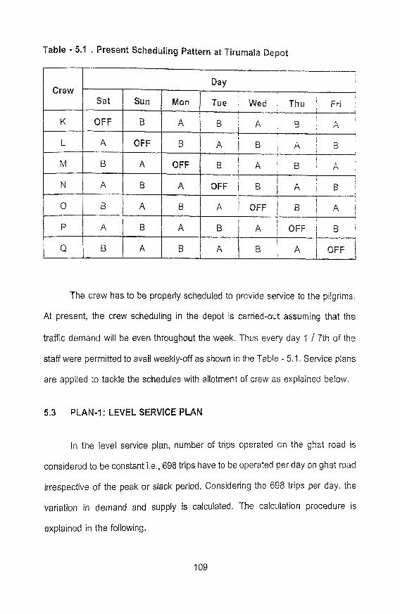
Table - 5.1 : Present Scheduling Pattern at Tirumala Depot
The crew has to be properly scheduled to provide service to the pilgrims.
At present, the crew scheduling in the depot is carried-out assuming that the
traffic demand will be even throughout the week. Thus every day 1 4 7th of the
staff were permitted to avail weekly-off as shown in the Table - 5.1. Service plans
are applied to tackle the schedules with allotment of crew as explained below.
5.3 PLAN-1 : LEVEL SERVICE PLAN
In the level service plan, number of trips operated on the ghat road is
considered to be constant i.e., 698 trips have to be operated per day on ghat road
irrespective of the peak or slack period. Considering the 698 trips per day, the
variation in demand and supply is calculated. The calculation procedure is
explained in the following.
5.33 Calculation of Variation in Demand
Notations used in this Chapter
nPk = no. of peak days In month
nSk = no. of slack days rn k"' month
pd, = average peak demand per day In k ' h m ~ t h
sd, = average slack demand per day In k" month
pDk = total peak demand In k" month
sDk = total slack demand in kt"' month
N ~ k = no. of trips operated in peak days in kt' month
Nsk = no. of trips operated in slack days in kt%month
Pv, = variation of peak demand and supply in k ' h o n t h
Sv, = variation of slack demand and supply in k" month
n = no. of passangers transported per trip
- Loss in peak period in k" month LP, -
LS, = Loss in slack period in kl%month
TL = Total Loss
Peak demand in kth month is
Slack demand in kth month is
sDk = n S , x s d ,
No. of passengers transported in peak perjod for 4" nonth zs
- N,, x nP, x n NP, -
No. of passengers transported in slack period for k'- rncnth 1s
Ns, = N , , , x n S , x n
Variation of peak demand and supply in kthmonth is
Pvk = Npk - PD,
Variation of slack demand and supply in kth month is
SPECIMEN CALCULATIONS
Based on the above steps, a sample calculation for the month of October - 1992 considering Table - 5.2, is explained below.
nPlo = 13; pd,, = 37053; n = 40; nS1, = 78.
sd,, = 29380; NDYlo = 698; N, 10 = 698;
Peak demand in October (pd,,) = nPdo x pd,,
- - 13 x 37053
Table - 5.2 : Demand Variation as per Plan-l
Slack demand in October (sd,,)
No. of passengers transported in peak period for October (Np,,)
No. of passengers transported in slack period for October (Ns,,)
Variation of peak demand
and supply in October(Pv,,)
- - -1,18,729
Negative sign -indicates demand is higher than the supply
Variation 9'; siack demand and = I \ $ S , ~ - S D : ~ supply in October (Sv,,)
Same procedure is followed for remaining months and the results are presented in Table - 5.2.
Table - 5 2 shows the number of peak days ~i siack. d a j s for eack ?cq:h
during 1992-93. The demand shown in column-5 gi3jes !he !o:ai i ~ n S e r 3!
pilgrims to be transported against each period The numbe: cf !rips cperated is
shown in column - 6 and the supply (the available faality) !or the traffic rs shavn
in column - 7. The variation shown in the last column sries :he bitefence
between supply and demand (1.e. difference behveen columns - 5 and 7). The
value with negatlve sign indicates that the organisaticn .s unable :o ~rc:'ide
service to the pilgr~rns. The value with positive sign indicates the number of empty
seats transported.
From the same Table - 5.2, rt can be observed that many times variation
is negative. In otherwords, the supply is less than the demand, thus incurring
some revenue losses to the organ~sation. The loss can be calculated by
considering various cost.
5.4 COST ESTIMATION
The cost parameters considered in the estimation sf costs are :
High speed diesel oil, Tyres cost, Spares cost and Depreciation.
The above costs are dependent on the krlornetres run. Hence the costs are
brought under variable cost which is calculated in running the vehicle per
Kilometre as explained below.
a. WSD Oil Cost
On ghat road section, a vehlcles consumes one litre of oil on an average
for running 4.4 Kilometres. The distance of ghat road section, Tirupati - T~rumala
and back, is 54 Kilometres (27 Km up and 27 Km down). So for running a vehicle
for one Kilometre in ghat road section, it needs 0.227 Litres (i.e., 114.4 L~tres) of
oil. The cost of HSD oil per litre is Rs. 6.89.
Cost per Kilometre on HSD PI
Cost of one litre of osl - -
No. of Kilometres travelled per litre a4
6.89 - - = 156 paise
4.4
(Indian Currency ; 1 Rupee = 108 p a w )
b. Tyres and Spares Cost
The cost spent on tyres for running the vehicle for one kilometre is
obtained as 71 paise and cost spent on spares is 41 paese: which are collected
from the record of stores.
c. Depreciation
Depreciation is fixed by the Head Office and is 71 paise per Kilometre.
d. Variable Cost
Total var~able cost is obtained by adding all the above costs per Kilometre.
a) Cost per K~lometre on HSD 011 = -156 parse
b) Tyre cost per Kilometre = 71 paise
c) Spares cost per K~lometre = 41 paise
d) Depreciation fixed by the Head Office (Management) per Kilometre = 71 paise
Total = 339 paise
= Rs. 3.39 paise
Total Kilometres from T~rupati bus stand to T~rumala bus stand = 27 K !cy-etres
Variable cost per Single = 232 ~ a ; s e x 27 ; T - ~
= 92 53 paise
= Rs 91 50 parse /say:
Variable cost per trip (2 singles)= 91.50 x 2 = 183
Variable cost per trip = Rs 283
Variable cost per passenger (vc) = (93.5'401 = Rs 2 28 (40 passengers bus capacity)
[trip = 2 singles (up and down)].
The organisation is running the vehicles at a net profit of Rs. 3 per
passenger (collected from the budget of the APSRTC).
i. If the variation is negative, i.e., demand is higher than the supply In such
case organisation is losing Rs. 3, because the passenger might have
chosen the alternate facility.
ii. If the variation is positive i.e., supply is higher than the demand, means
that the vehicles are run with vacant seats. So the organisation is Ios~ng
the variable cost Rs. 2. 28 per seat. In both the cases, the organisation IS
losing some revenue which is shown below.
Loss in peak period for kth month is
L ~ k = PV, x r
Where (profit) r = Rs. 3 for - ve variation or Rs. 2.28 or + ve variation
Loss in slack period for kth month is
Ls, = Sv, x r
e , L"n:q?L- e"t~e7:~:: The cost of the ticket per passenger is Rs. 12 But. ti.^ -. profit per passenger (pilgrim) is Rs. 3 (this has been obtained from t?e '"!x?-;e:
and project~ons" of APSRTC). The profit and loss calcuiatioos a5a:n.i eacr
passenger are shown below considering the demand variat~or,.
I. 0 Variation
Demand of passengers = 1CO
Ava~lab~lity of number of seats I
Passengers transported
(i.e , service provided) = ?OO
Net profit = 108x3 =Rs 300
2. -ve variation Demand of passengers
Availability of number of seats f
Passengers transported
(i.e., service provided) = 100
Profit = 1 0 0 x 3 =Rs 300
But if we extend the transportation facilities to 150 passengers, then the
profit would be Rs. 450 (i.e., 150 x 3).
Reduction in profit
Therefore, we consider this Rs.150 as loss due to non-availability of
required service level
3. +we variation
Demand of passengers - - 53
Availability of number of seats - - Z CO Passengers transported - - 59
(i.e., service provided)
Profit - - 53 x 3 = Rs. "J50
Var~able cost of providing passenger service at
Rs. 2. 28 per seat is 2. 28 x 50 = Rs 'I 94
Hence the net profit = 150 - 114 = Rs. 36
SPECIMEN CALCULATIONS
Sample calculation for the month of October is explained below
Loss in peak period (Lp,,) = (PV,~) x F
= Rs. 3,56,187
Loss in slack period (Ls,,) = Sv,, x r
Same procedure is followed for remaining months and are shown in Table - 5.3.
Total loss for the financial year is 12
Total loss = q L p , + Ls,) k= 1
= Rs. 39,54,882
In this context, the above amount is to be considere? as css cxx3~ 13:
mean that the Depot is to run at loss but there is a scnce :c :-zreas2 :-.e C--?::S
by proper scheduling or by allow~ng overtime
Table - 5.3 : Profit and Loss as per Plan-l
A P ~ Peak 1 -68112 2~4336 Slack + 83466 , 190362
Month
I
Peak - 10764 32292 1 Slack + 182790 1 234361
Total expected loss Rs. 39,54,855
119
Period Variation Loss in Rs. I
5.5 PLAN - 2: LEVEL SERVICE PLAN WITH OVERTIME
If extra tr~ps are operated by the organisa1:sn. :a Pas :: ca: s,er t . ~ e t lc j
drivers. The cost incurred per trip In over time 1s Rs 66; So esst per
passenger will come to Rs. 0.75. Even thohigh by operatrrc extra C Y ~ S , 1? IS f i ~ f
possible to clear all the passengers for want of time w:th th,e Sset S~ZF? acd some
of the p~lgr~rns reach by alternate faciilties. By operatirig extra tirips. ,t is possibfe
only 50% of the people can be transported. This cvertjme :rigs are o3erated xhen
the variation is negative. The loss can be calculated by .jsir.g the f~li@:/rkig
equation.
Loss in peak period for kt%onth is
r a x m x P v ,
I (vc) x Pv,
- ve variation
+ ve variation
Loss in slack period for kt%month is
a x m x SV, - ve variation
(vc) x Sv, + ve variation
Where a = operating extra trips = 50% = 8.5
m = cost incurred per trip in over time = Rs. 0.75
Total loss is
TL (LP, * LsJ
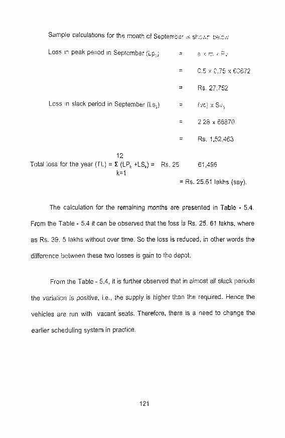
Sample calculattons for the month of September I S sh:r.r ke:::;
Loss in peak per~od in September (Lp ; - - 3 y ~y ,d ?:
= C.5 x 0.75 x 6CSJ2
= Ws. 27,752
Loss in slack period in September (Ls,) - - Ivc) x St!;
= Rs. 1,52,46@
12 Total loss for the year (TL) = E (LP, +LS,j = Rs. 25 61,496
k= l = Rs. 25.61 lakhs (say).
The calculation for the remaining months are presented in Table - 5.4.
From the Table - 5.4 it can be observed that the loss is Rs. 25. 61 takhs, where
as Rs. 39. 5 lakhs without over time. So the loss is reduced, in other words the
difference between these two losses is gain to the depot.
From the Table - 5.4, it is further observed that in almost all slack periods
the variation is positive, i.e., the supply is higher than the required. Hence the
vehicles are run with vacant seats. Therefore, there is a need to change the
earlier scheduling system in practice.
Table - 5.4 : Profit and Loss as per Plan - 2
Total expected loss Rs. 25,61,496 25.61 takhs
5.6 PLAN - 3 : CHASE PLAN
Keen observation of both the plans reveals that tho 5snand *s l.'acflqg
greatly as much as 30% behnreen peak days and slack days in a iaieeC.. . Thus,
there is a mismatch between traffic demand and supply of buses and the crew.
To overcome this situation, few changes have been made in scheduling of the
KEYS. Weekly-offs are cancelled on peak days, i.e., on Saturdays. Sundays and
Mondays Instead, weekly-off are provided during the slack days of the week.
Thus facilitating all the crew available for duties in peak days. The revised
scheduling chart is shown in Table - 5.5.
Table - 5.5 : Proposed scheduling pattern for Tirumala depot.
Q [ A I
B l A I
B I A B 1 OFF
By the above suggested method of scheduling, 45 extra trips have been
achieved in peak periods and 45 less trips in slack periods. Thus in peak periods,
there was a total of (698 + 45) = 743 trips per day operated on ghat road and on
slack days (698-45) = 653 trips. By operating 743 trips in peak periods and 653
in slack periods, the var~atron between demand and srp;ly IS c a - Ibdlated fz: the
month of April, as shown in the follow~ng. The same piace?-re :s fc;la::eS a-:' :he
results are presented in Table - 5.6.
n = 40 (Capacity of a Bus and over load is not permitted on Ghat Aaadj
nS, = 18 sd, = 23283 N5.4 - - 653
Peak demsnd in April (pD,) = nP, x
= 12 x 33596 = 4,03,152
Slack demand in April (sD,) = nS, x sd,
No. of passengers transported in peak period for April (Np,)
No. of passengers transported in = hisv4 x nS, x n slack period for April (Ns,)
Variation of peak demand and supply ' NP, - PD, in April (Pv,)
Variation of slack demand and supply = Ns, - s5, in April (Sv,)
= 4701 60 - 41 9094 = 511,066
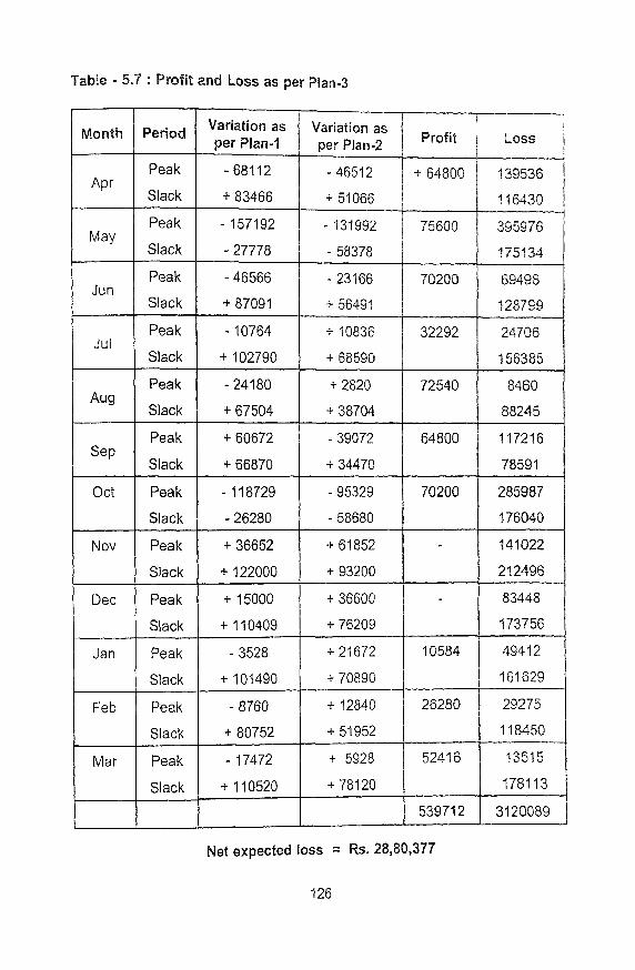
The profit and loss calculations are shown in Table - 5.7. In this plan, the loss
is reduced to Rs. 25.80 lakhs when compared to Rs. 39.5 lakhs as per Plan-l.
Table - 5.6 : Variation in Demand and Supply as per Plan - 3
Table - 5.7 : Profit and Loss as per Plan9
Net expected loss = Rs. 28,80,377
126
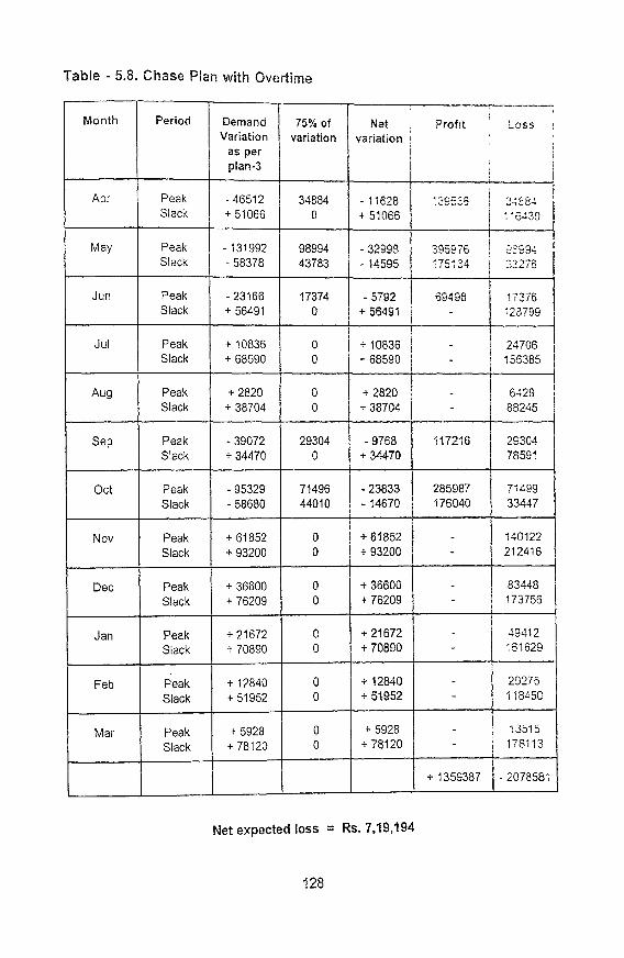
5.7 PLAN - 4: CHASE PLAN WITH BVERTIME
Plan-3 can further be refined by allowing overtlme as i: has Liz&- 23;;"- U G
Plan-2. By allowing overtime, it is possible to clear 7SC2 cf :he re"rza:?xg
passengers due to development of more number of busses and csel::
The profit and loss calculation for this plan is sh8:w !n Tabl'e - 5 2 As oe:
this plan, the loss can be reduced to Rs 7.2 Lakhs in csmpaslson to Ss 39 5
Lakhs in Plan-?, which is a significant gain.
The comparative reduction of loss due to mismatch~ng of demand and
supply for all the plans discussed in the foregone pages is shown in Figure - 5.1.
which is self explanatory.
Table - 5.8. Chase Plan with Overtime
Net I Profrt Loss i
Net expected loss = Rs. 7,19,194
128
5.8 VALIDATION
The demand generated by cons;denn(j 5'i 5:~;::: . z : ~ ;z-:ie rq,:' - 3 ~ 3 : 2 ~
year is validated by using F~sher d~str~butlon to f:nd ~:.h&-+er :rere is a s ,::- '- a.paz:
difference between the actual demand pattern and Corecaste^, ~ e m a z ? patlei-n
The calculation procedure is explained below:
Of X,, X, .... X, and Y,, Y,. ..Y, be the values of indepencent razdorn
samples drawn from the same normal population with variance d
Then F IS defined by the relation
1 n, Where S, = E (x,-x)*
n,-I 1-1
Where x, y are sample means.
The value of F corresponding to significant level and degrees of freedom
to each sample is taken from the statistical table. The value obtained by the
equation is compared with the above statistical table value. If the value fails within
the table value the null hypothesis is accepted or true sthenvise the null
hypothesis is rejected.
Null Hypothesis
There is no significant d~fference in variance . t . u ~ ~ ~ ; ~ ' ; ~ : : ::+" ?--:
actual demand
X, = Total forecasted demand in ~'"eerlod
Y, = Total actual demand in lt\miOd
* Ex The average forecasted demand X =
n,
C TYI The average actual demand Y - -
n,
The variance of forecasted demand is
The variance of actual demand IS
The F~sher F Constant IS
From the table at 75%. confidence level at r, = n,-l = 11
r2 = n,-1 = 12-11 = 1, the value F,, = 2.82
Hence, the calculated F value is less than tRe table value. So the null
hypothesis is accepted, i.e., there is no significant variation between actual and
forecasted demand.
, in this Chapter, the four methods adopted to increase the revenue is
explained systematically. A 5% growth rate in the pilgrim traffic has been
assumed and the demand estimated for the next financial year, so as to adjust
the available fleet to meet the demand. The Fisher's distribution is used to
validate the model and found to be within the limits. Thus the methodology is
validated satisfactorily.
The plan-4 is implemented at Tirumala Depot. With the ~mplementation of
the above plan, the incremental losses due to non-transportat~on of pilgr~ms on
peak periods and loss due to operating of empty trips on slack periods have been
brought to rock bottom, thereby greatly increasing the revenue of the depot. The
actual revenue earned are shown in Table - 5.9 and Figure - 5.2 by the
lmplementat~on of Plan - 4 (as furnished by the APSRTCJ. From the table it can
be observed that the revenue during 1992-93 was only Rs. 456.1 lakhs. On
implementation of the Plan - 4, the revenue is almost is rised by four times during
1993-94. But this was only twice during 1993-94 when compared to 1991 -92. As
such the initial attempt made by the author implement Aggregate Planning
techniques in the practical situation is found to be successful. To run and
implement such decisions, reliability of the system is needed. Therefore the
rsliability relating to the present context is presented in the next chapter.
Table - 5.9 : Revenue at Tiaumala Depot from 1991 to 1997