68
Aggregate Planning Chapter 11
| Date post: | 05-Jan-2016 |
| Category: |
Documents |
| Upload: | stewart-hudson |
| View: | 239 times |
| Download: | 1 times |

Aggregate Planning
Chapter 11

Aggregate Planning
• Aggregate planning– Intermediate-range capacity planning that typically covers a
time horizon of 2 to 18 months.– Useful for organizations that experience seasonal, or other
variations in demand.– “Big-picture” approach. Groups together similar products
(services) and deals with them as though they were a single products (service).
– Goal:• Achieve a production plan that will effectively utilize the
organization’s resources to satisfy overall demand

The Planning Sequence
Long-term planning
Intermediate-term planning
Short-term detailed planning
Aggregate Planning
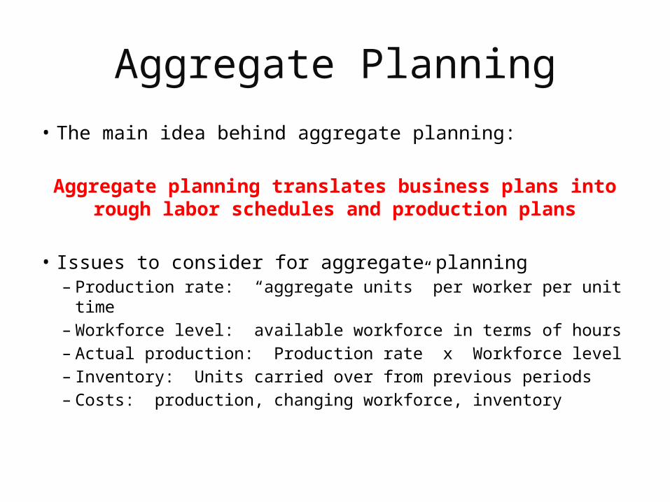
• The main idea behind aggregate planning:
Aggregate planning translates business plans into rough labor schedules and production plans
• Issues to consider for aggregate planning– Production rate: “aggregate units” per worker per unit time– Workforce level: available workforce in terms of hours– Actual production: Production rate x Workforce level– Inventory: Units carried over from previous periods– Costs: production, changing workforce, inventory
What does aggregate planning do?
• Given an aggregate demand forecast, determine production levels, inventory levels, and workforce levels, in order to minimize total relevant costs over the planning horizon
Why do organizations need to do aggregate planning?
• Planning– It takes time to implement plans (e.g. hiring).
• Aggregation– It is not possible to predict with accuracy the timing and volume of
demand for individual items.
• Planning is connected to the budgeting process which is usually done annually on an aggregate (e.g., departmental) level.
• It can help synchronize flow throughout the supply chain; it affects costs, equipment utilization; employment levels; and customer satisfaction
Aggregate Planning Strategies
• Proactive– Alter demand to match supply (capacity)– Among other approaches, we can alter demand by
simply changing the price.• Reactive
– Alter supply (capacity) to match demand– Through capacity planning and aggregate planning
• Mixed– Some of each

Demand Options• Pricing
– Used to shift demand from peak to off-peak periods.• Airline: night/weekend• Restaurants: happy hour/early bird
– Price elasticity is important– Yield (Revenue) Management
• Maximizing revenue by using a variable pricing strategy. Prices are set relative to capacity availability.
• Promotion– Advertising and other forms of promotion– Issue: response rate and response patterns. Less control over timing of demand (may
worsen the problem by bringing demand at the wrong time).
• Back orders (delaying order filling)– Orders are taken in one period and deliveries promised for a later period– Possible loss of sales, increased record keeping, lowered customer service level
• New demand– Very uneven situation– Offer different products/services during off-peak periods to make use of excess capacity:
fastfood stores offer breakfast.
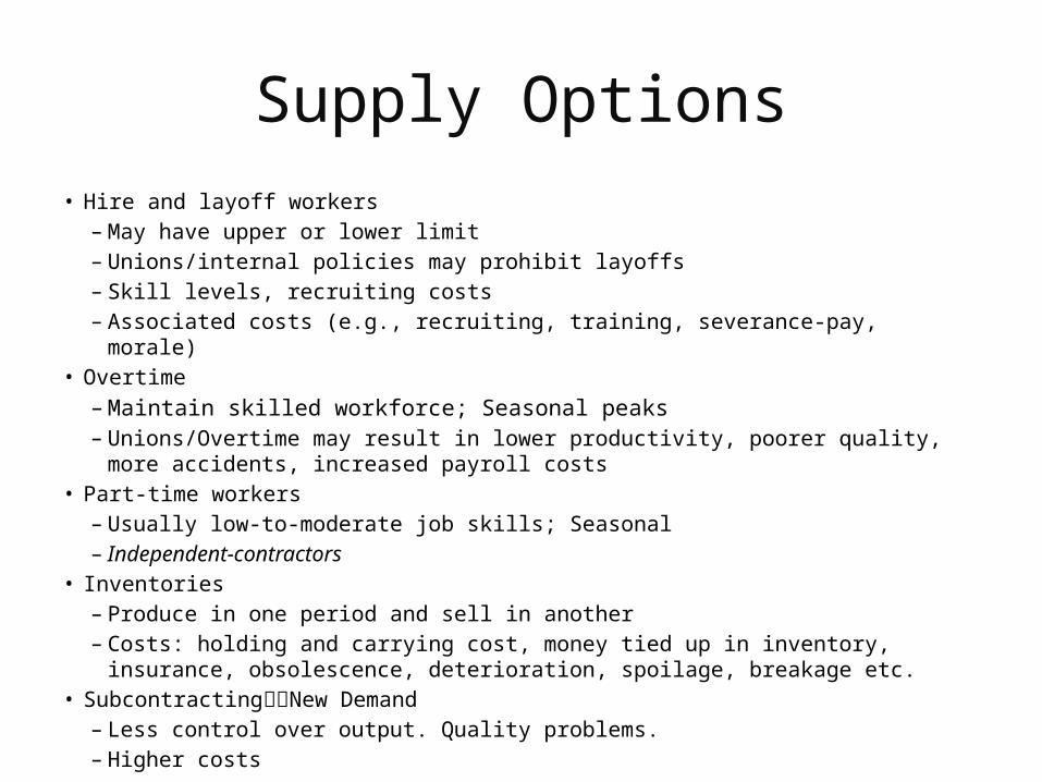
Supply Options• Hire and layoff workers
– May have upper or lower limit– Unions/internal policies may prohibit layoffs– Skill levels, recruiting costs– Associated costs (e.g., recruiting, training, severance-pay, morale)
• Overtime– Maintain skilled workforce; Seasonal peaks– Unions/Overtime may result in lower productivity, poorer quality, more accidents,
increased payroll costs• Part-time workers
– Usually low-to-moderate job skills; Seasonal– Independent-contractors
• Inventories– Produce in one period and sell in another– Costs: holding and carrying cost, money tied up in inventory, insurance, obsolescence,
deterioration, spoilage, breakage etc.• SubcontractingNew Demand
– Less control over output. Quality problems. – Higher costs

MIS 373: Basic Operations Management
11
Aggregate Planning Supply Strategies
• Level capacity strategy: – Maintaining a steady rate of regular-time output;
variations in demand are met by using inventories or other options such as overtime, part-time workers, subcontracting, and backorders
• Chase demand strategy: – Matching capacity to demand; the planned output for a
period is set at the expected demand for that period.

MIS 373: Basic Operations Management
12
Level strategy
• Capacities are kept constant over the planning horizon– Advantages
• Stable output rates and workforce
– Disadvantages• Greater inventory (or other) costs

MIS 373: Basic Operations Management
13
Chase strategy
• Capacities are adjusted to match demand requirements over the planning horizon– Advantages
• Investment in inventory is low• Labor utilization in high
– Disadvantages• The cost of adjusting output rates and/or workforce levels

Uneven Demand and Two Strategies:
11-14
Demand = Supply Demand < Supply Demand > Supply
Supply (output) level

MIS 373: Basic Operations Management
15
Choosing a Strategy
• Important factors:– Company policy
• Constraints on the available options– e.g., discourage layoffs, no subcontracting to protects secrets, union
policies regarding over time
– Flexibility• Chase flexibility may not be present for companies designed for
high steady output (e.g., refineries, auto assembly)
– Cost• Alternatives are evaluated in term of cost (while matching demand
within the constraints).

Trial-and-Error Techniques
• Trial-and-error approaches consist of developingsimple table or graphs that enable planners to visually compare projected demand requirements with existing capacity
• Alternatives are compared based on their total costs
• Disadvantage:– it does not necessarily result in an optimal aggregate plan
MIS 373: Basic Operations Management
17
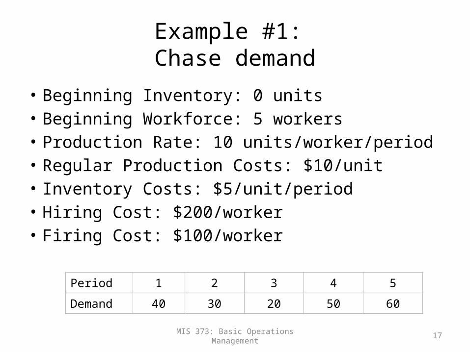
Example #1: Chase demand
• Beginning Inventory: 0 units• Beginning Workforce: 5 workers• Production Rate: 10 units/worker/period• Regular Production Costs: $10/unit• Inventory Costs: $5/unit/period• Hiring Cost: $200/worker• Firing Cost: $100/worker
Period 1 2 3 4 5Demand 40 30 20 50 60
MIS 373: Basic Operations Management
18
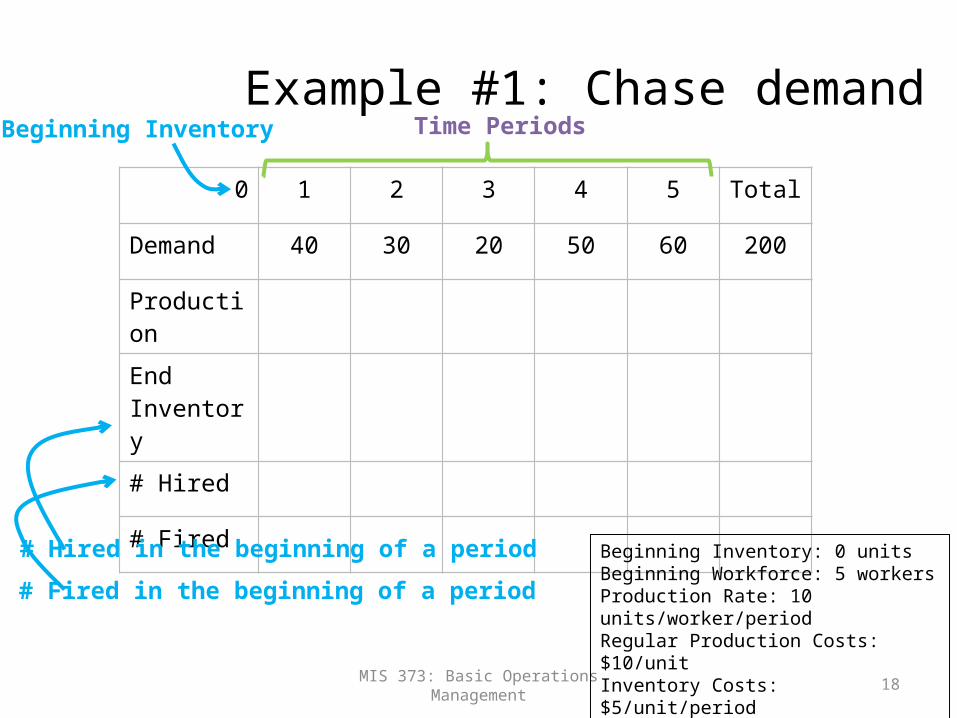
Example #1: Chase demand
0 1 2 3 4 5 Total
Demand 40 30 20 50 60 200
Production
End Inventory
# Hired
# Fired
Beginning Inventory: 0 unitsBeginning Workforce: 5 workersProduction Rate: 10 units/worker/periodRegular Production Costs: $10/unitInventory Costs: $5/unit/periodHiring Cost: $200/workerFiring Cost: $100/worker
Beginning Inventory Time Periods
# Hired in the beginning of a period
# Fired in the beginning of a period
MIS 373: Basic Operations Management
19
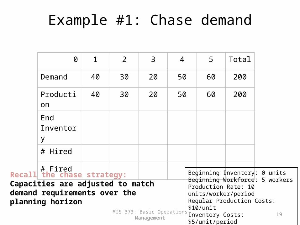
Example #1: Chase demand
0 1 2 3 4 5 Total
Demand 40 30 20 50 60 200
Production 40 30 20 50 60 200
End Inventory
# Hired
# Fired
Beginning Inventory: 0 unitsBeginning Workforce: 5 workersProduction Rate: 10 units/worker/periodRegular Production Costs: $10/unitInventory Costs: $5/unit/periodHiring Cost: $200/workerFiring Cost: $100/worker
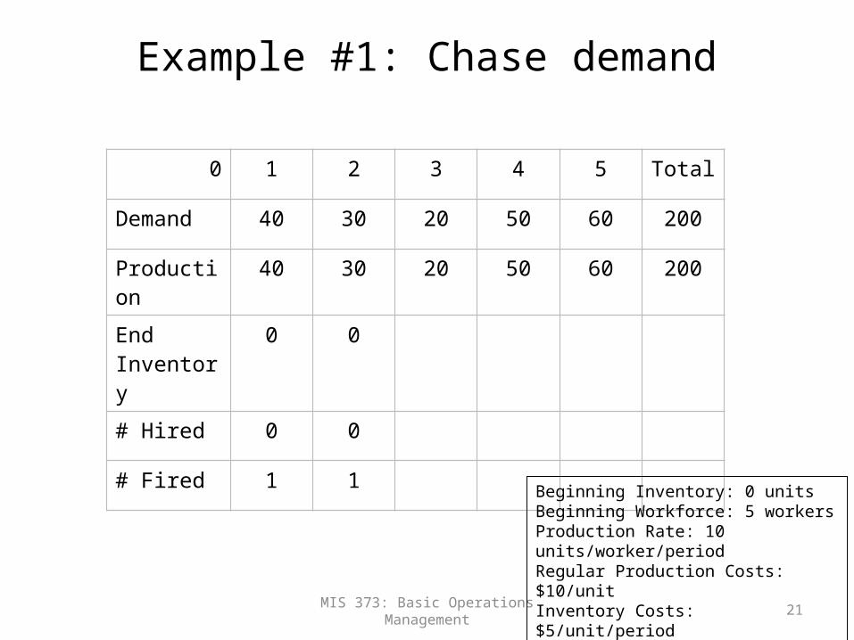
Recall the chase strategy: Capacities are adjusted to match demand requirements over the planning horizon

MIS 373: Basic Operations Management
20
Example #1: Chase demand
0 1 2 3 4 5 Total
Demand 40 30 20 50 60 200
Production 40 30 20 50 60 200
End Inventory
0
# Hired 0
# Fired 1
Beginning Inventory: 0 unitsBeginning Workforce: 5 workersProduction Rate: 10 units/worker/periodRegular Production Costs: $10/unitInventory Costs: $5/unit/periodHiring Cost: $200/workerFiring Cost: $100/worker
MIS 373: Basic Operations Management
21
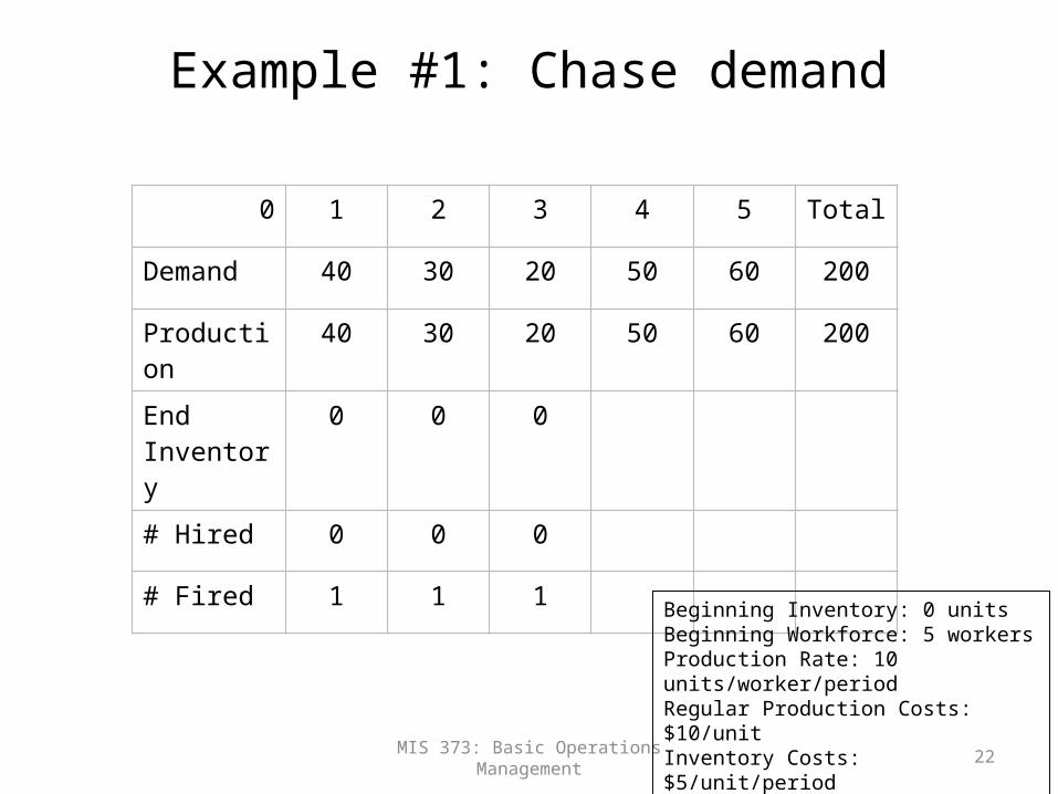
Example #1: Chase demand
0 1 2 3 4 5 Total
Demand 40 30 20 50 60 200
Production 40 30 20 50 60 200
End Inventory
0 0
# Hired 0 0
# Fired 1 1
Beginning Inventory: 0 unitsBeginning Workforce: 5 workersProduction Rate: 10 units/worker/periodRegular Production Costs: $10/unitInventory Costs: $5/unit/periodHiring Cost: $200/workerFiring Cost: $100/worker
MIS 373: Basic Operations Management
22
Example #1: Chase demand
0 1 2 3 4 5 Total
Demand 40 30 20 50 60 200
Production 40 30 20 50 60 200
End Inventory
0 0 0
# Hired 0 0 0
# Fired 1 1 1
Beginning Inventory: 0 unitsBeginning Workforce: 5 workersProduction Rate: 10 units/worker/periodRegular Production Costs: $10/unitInventory Costs: $5/unit/periodHiring Cost: $200/workerFiring Cost: $100/worker
MIS 373: Basic Operations Management
23
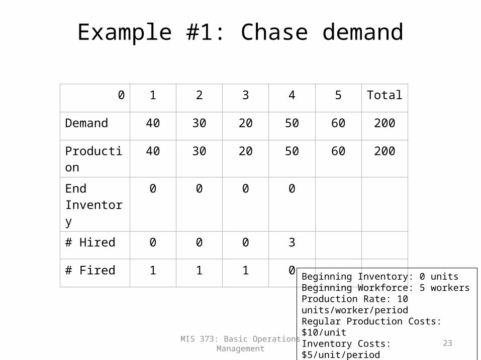
Example #1: Chase demand
0 1 2 3 4 5 Total
Demand 40 30 20 50 60 200
Production 40 30 20 50 60 200
End Inventory
0 0 0 0
# Hired 0 0 0 3
# Fired 1 1 1 0
Beginning Inventory: 0 unitsBeginning Workforce: 5 workersProduction Rate: 10 units/worker/periodRegular Production Costs: $10/unitInventory Costs: $5/unit/periodHiring Cost: $200/workerFiring Cost: $100/worker

MIS 373: Basic Operations Management
24
Example #1: Chase demand
0 1 2 3 4 5 Total
Demand 40 30 20 50 60 200
Production 40 30 20 50 60 200
End Inventory
0 0 0 0 0
# Hired 0 0 0 3 1
# Fired 1 1 1 0 0
Beginning Inventory: 0 unitsBeginning Workforce: 5 workersProduction Rate: 10 units/worker/periodRegular Production Costs: $10/unitInventory Costs: $5/unit/periodHiring Cost: $200/workerFiring Cost: $100/worker
MIS 373: Basic Operations Management
25
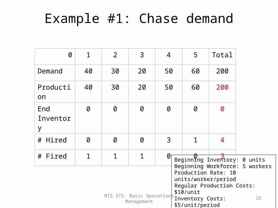
Example #1: Chase demand
0 1 2 3 4 5 Total
Demand 40 30 20 50 60 200
Production 40 30 20 50 60 200
End Inventory
0 0 0 0 0 0
# Hired 0 0 0 3 1 4
# Fired 1 1 1 0 0 3
Beginning Inventory: 0 unitsBeginning Workforce: 5 workersProduction Rate: 10 units/worker/periodRegular Production Costs: $10/unitInventory Costs: $5/unit/periodHiring Cost: $200/workerFiring Cost: $100/worker
MIS 373: Basic Operations Management
26
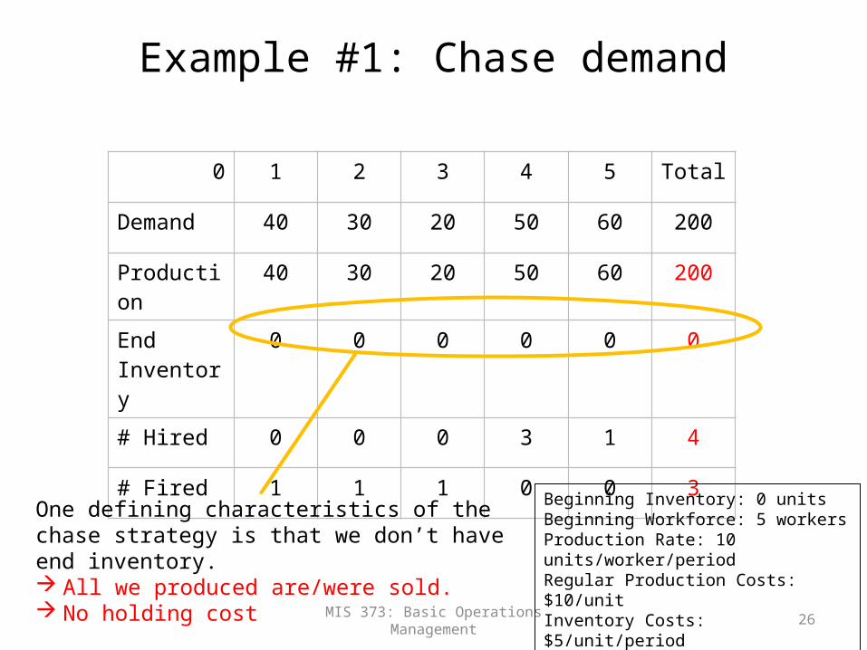
Example #1: Chase demand
0 1 2 3 4 5 Total
Demand 40 30 20 50 60 200
Production 40 30 20 50 60 200
End Inventory
0 0 0 0 0 0
# Hired 0 0 0 3 1 4
# Fired 1 1 1 0 0 3
Beginning Inventory: 0 unitsBeginning Workforce: 5 workersProduction Rate: 10 units/worker/periodRegular Production Costs: $10/unitInventory Costs: $5/unit/periodHiring Cost: $200/workerFiring Cost: $100/worker
One defining characteristics of the chase strategy is that we don’t have end inventory. All we produced are/were sold. No holding cost
MIS 373: Basic Operations Management
27
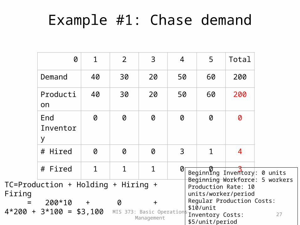
Example #1: Chase demand
0 1 2 3 4 5 Total
Demand 40 30 20 50 60 200
Production 40 30 20 50 60 200
End Inventory
0 0 0 0 0 0
# Hired 0 0 0 3 1 4
# Fired 1 1 1 0 0 3
Beginning Inventory: 0 unitsBeginning Workforce: 5 workersProduction Rate: 10 units/worker/periodRegular Production Costs: $10/unitInventory Costs: $5/unit/periodHiring Cost: $200/workerFiring Cost: $100/worker
TC=Production + Holding + Hiring + Firing = 200*10 + 0 + 4*200 + 3*100 = $3,100

Exercise
• Perform aggregate planning using the chase strategy:– Beginning Inventory: 10 units– Beginning Workforce: 5 workers– Production Rate: 10 units/worker/period– Regular Production Costs: $10/unit– Inventory Costs: $10/unit/period– Hiring Cost: $100/worker– Firing Cost: $200/workerPeriod 1 2 3 4 5Demand 50 40 30 30 40
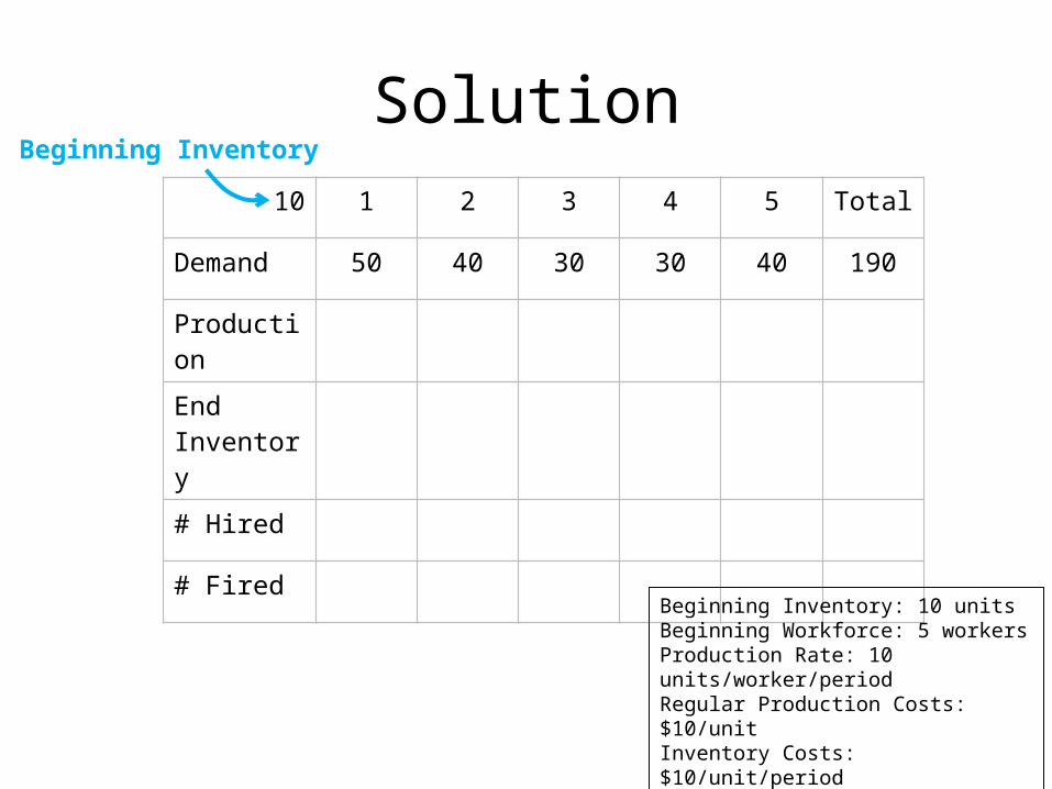
10 1 2 3 4 5 Total
Demand 50 40 30 30 40 190
Production
End Inventory
# Hired
# Fired
Beginning Inventory: 10 unitsBeginning Workforce: 5 workersProduction Rate: 10 units/worker/periodRegular Production Costs: $10/unitInventory Costs: $10/unit/periodHiring Cost: $100/workerFiring Cost: $200/worker
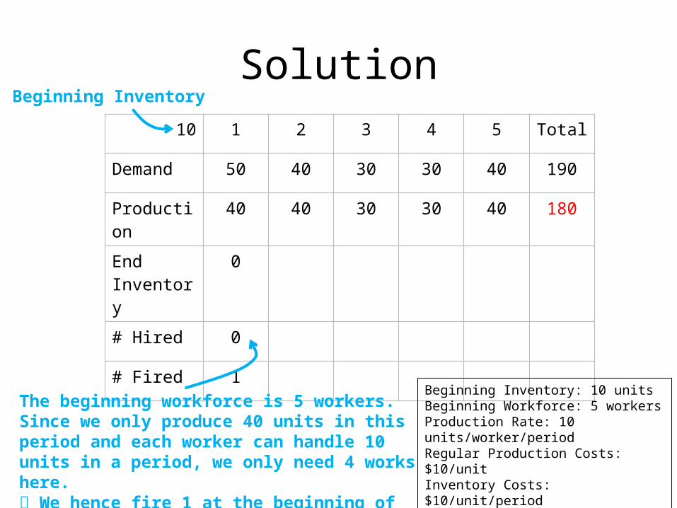
Beginning InventorySolution

10 1 2 3 4 5 Total
Demand 50 40 30 30 40 190
Production 40 40 30 30 40 180
End Inventory
# Hired
# Fired
Beginning Inventory: 10 unitsBeginning Workforce: 5 workersProduction Rate: 10 units/worker/periodRegular Production Costs: $10/unitInventory Costs: $10/unit/periodHiring Cost: $100/workerFiring Cost: $200/worker
Beginning Inventory
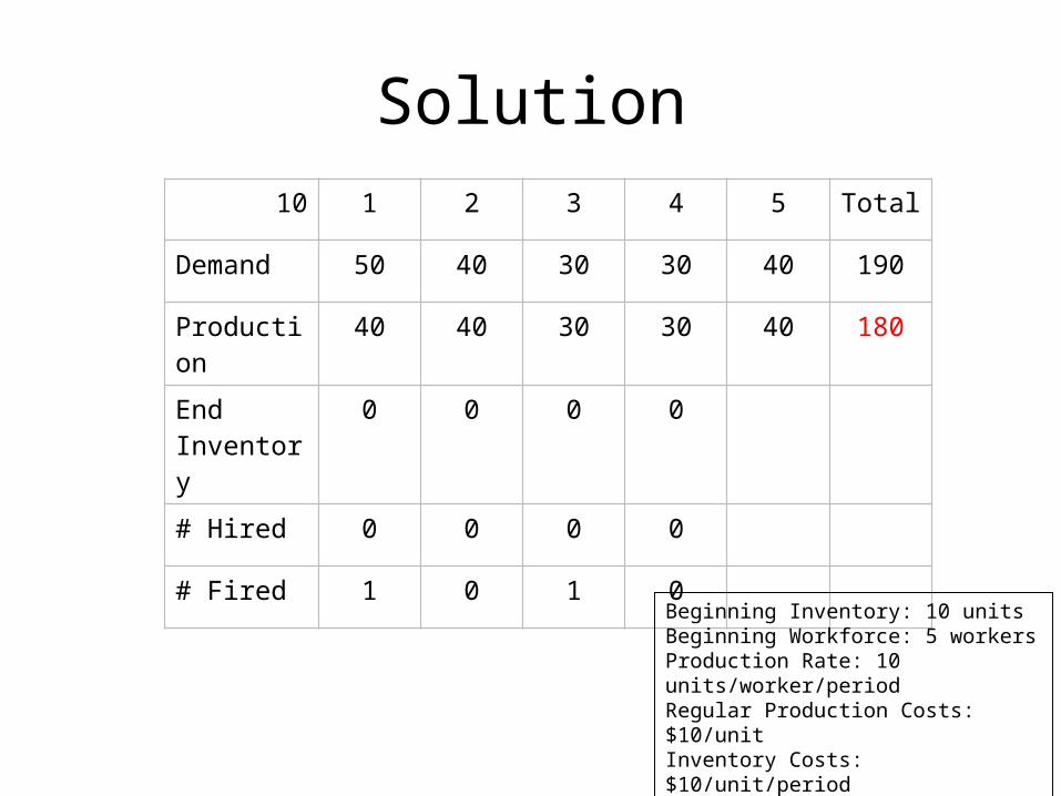
We only produce 40 units because there are 10 units beginning inventory that we can use.So, we can still meet the demand of 50 units.
Solution
10 1 2 3 4 5 Total
Demand 50 40 30 30 40 190
Production 40 40 30 30 40 180
End Inventory
0
# Hired 0
# Fired 1
Beginning Inventory: 10 unitsBeginning Workforce: 5 workersProduction Rate: 10 units/worker/periodRegular Production Costs: $10/unitInventory Costs: $10/unit/periodHiring Cost: $100/workerFiring Cost: $200/worker
Beginning Inventory
The beginning workforce is 5 workers. Since we only produce 40 units in this period and each worker can handle 10 units in a period, we only need 4 works here. We hence fire 1 at the beginning of this period.
Solution

10 1 2 3 4 5 Total
Demand 50 40 30 30 40 190
Production 40 40 30 30 40 180
End Inventory
0 0
# Hired 0 0
# Fired 1 0
Beginning Inventory: 10 unitsBeginning Workforce: 5 workersProduction Rate: 10 units/worker/periodRegular Production Costs: $10/unitInventory Costs: $10/unit/periodHiring Cost: $100/workerFiring Cost: $200/worker
Solution

10 1 2 3 4 5 Total
Demand 50 40 30 30 40 190
Production 40 40 30 30 40 180
End Inventory
0 0 0
# Hired 0 0 0
# Fired 1 0 1
Beginning Inventory: 10 unitsBeginning Workforce: 5 workersProduction Rate: 10 units/worker/periodRegular Production Costs: $10/unitInventory Costs: $10/unit/periodHiring Cost: $100/workerFiring Cost: $200/worker
Solution
10 1 2 3 4 5 Total
Demand 50 40 30 30 40 190
Production 40 40 30 30 40 180
End Inventory
0 0 0 0
# Hired 0 0 0 0
# Fired 1 0 1 0
Beginning Inventory: 10 unitsBeginning Workforce: 5 workersProduction Rate: 10 units/worker/periodRegular Production Costs: $10/unitInventory Costs: $10/unit/periodHiring Cost: $100/workerFiring Cost: $200/worker
Solution

10 1 2 3 4 5 Total
Demand 50 40 30 30 40 190
Production 40 40 30 30 40 180
End Inventory
0 0 0 0 0 0
# Hired 0 0 0 0 1 1
# Fired 1 0 1 0 0 2
Beginning Inventory: 10 unitsBeginning Workforce: 5 workersProduction Rate: 10 units/worker/periodRegular Production Costs: $10/unitInventory Costs: $10/unit/periodHiring Cost: $100/workerFiring Cost: $200/worker
TC=Production + Holding + Hiring + Firing = 180*10 + 5*10 + 1*100 + 2*200
Solution

MIS 373: Basic Operations Management
37
Example #2: Level Capacity
0 1 2 3 4 5 Total
Demand 40 30 20 50 60 200
Production
End Inventory
# Hired
# Fired
Beginning Inventory: 0 unitsBeginning Workforce: 5 workersProduction Rate: 10 units/worker/periodRegular Production Costs: $10/unitInventory Holding Costs: $5/unit/periodHiring Cost: $200/workerFiring Cost: $100/worker
MIS 373: Basic Operations Management
38
Example #2: Level Capacity
0 1 2 3 4 5 Total
Demand 40 30 20 50 60 200
Production 40 40 40 40 40 200
End Inventory
# Hired
# Fired
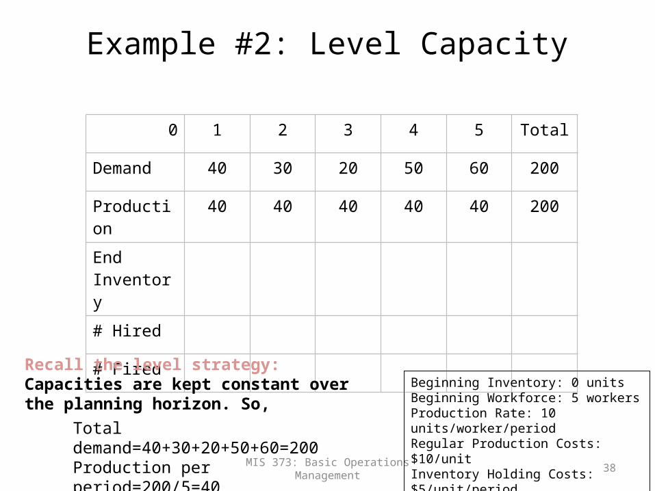
Total demand=40+30+20+50+60=200Production per period=200/5=40
Beginning Inventory: 0 unitsBeginning Workforce: 5 workersProduction Rate: 10 units/worker/periodRegular Production Costs: $10/unitInventory Holding Costs: $5/unit/periodHiring Cost: $200/workerFiring Cost: $100/worker
Recall the level strategy: Capacities are kept constant over the planning horizon. So,
MIS 373: Basic Operations Management
39
Example #2: Level Capacity
0 1 2 3 4 5 Total
Demand 40 30 20 50 60 200
Production 40 40 40 40 40 200
End Inventory
0
# Hired 0
# Fired 1
Beginning Inventory: 0 unitsBeginning Workforce: 5 workersProduction Rate: 10 units/worker/periodRegular Production Costs: $10/unitInventory Holding Costs: $5/unit/periodHiring Cost: $200/workerFiring Cost: $100/worker

MIS 373: Basic Operations Management
40
Example #2: Level Capacity
0 1 2 3 4 5 Total
Demand 40 30 20 50 60 200
Production 40 40 40 40 40 200
End Inventory
0
# Hired 0
# Fired 1
Beginning Inventory: 0 unitsBeginning Workforce: 5 workersProduction Rate: 10 units/worker/periodRegular Production Costs: $10/unitInventory Holding Costs: $5/unit/periodHiring Cost: $200/workerFiring Cost: $100/worker
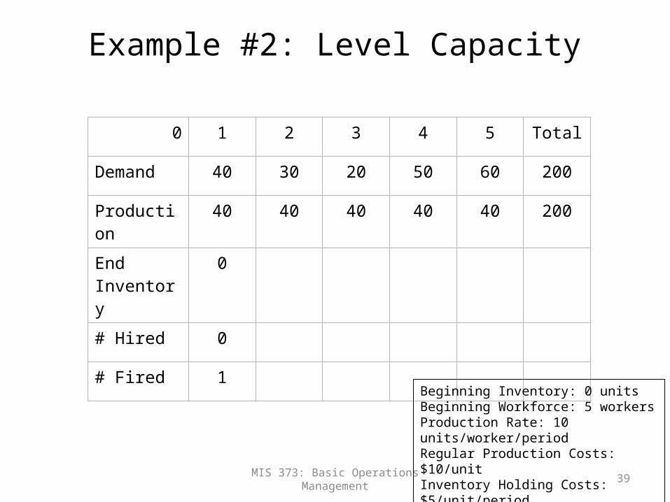
Fire 1 worker in this period because 4 workers are sufficient to produce 40 units in a period.

MIS 373: Basic Operations Management
41
Example #2: Level Capacity
0 1 2 3 4 5 Total
Demand 40 30 20 50 60 200
Production 40 40 40 40 40 200
End Inventory
0 10
# Hired 0 0
# Fired 1 0
Beginning Inventory: 0 unitsBeginning Workforce: 5 workersProduction Rate: 10 units/worker/periodRegular Production Costs: $10/unitInventory Holding Costs: $5/unit/periodHiring Cost: $200/workerFiring Cost: $100/worker
MIS 373: Basic Operations Management
42
Example #2: Level Capacity
0 1 2 3 4 5 Total
Demand 40 30 20 50 60 200
Production 40 40 40 40 40 200
End Inventory
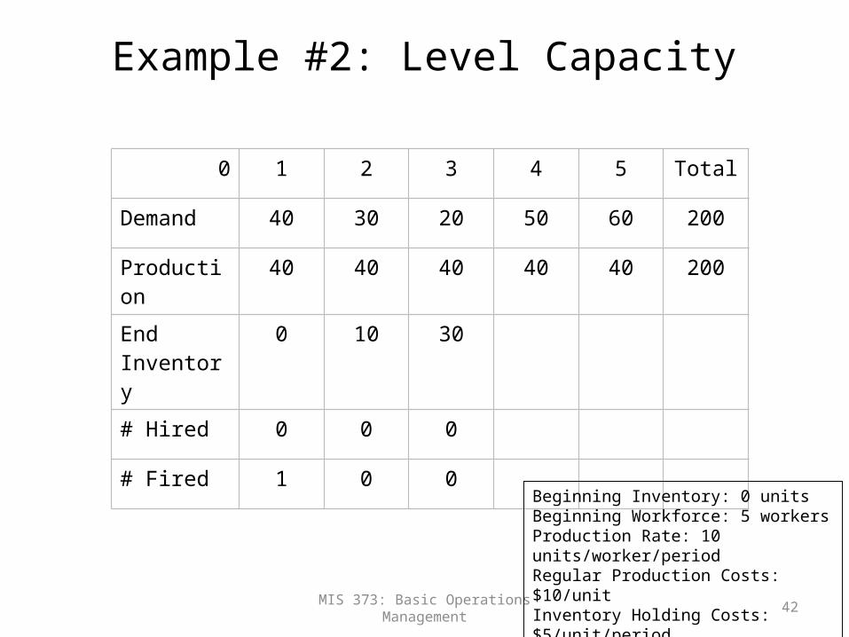
0 10 30
# Hired 0 0 0
# Fired 1 0 0
Beginning Inventory: 0 unitsBeginning Workforce: 5 workersProduction Rate: 10 units/worker/periodRegular Production Costs: $10/unitInventory Holding Costs: $5/unit/periodHiring Cost: $200/workerFiring Cost: $100/worker

MIS 373: Basic Operations Management
43
Example #2: Level Capacity
0 1 2 3 4 5 Total
Demand 40 30 20 50 60 200
Production 40 40 40 40 40 200
End Inventory
0 10 30 20
# Hired 0 0 0 0
# Fired 1 0 0 0
Beginning Inventory: 0 unitsBeginning Workforce: 5 workersProduction Rate: 10 units/worker/periodRegular Production Costs: $10/unitInventory Holding Costs: $5/unit/periodHiring Cost: $200/workerFiring Cost: $100/worker
MIS 373: Basic Operations Management
44
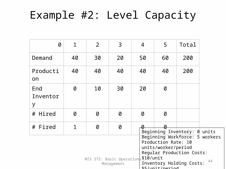
Example #2: Level Capacity
0 1 2 3 4 5 Total
Demand 40 30 20 50 60 200
Production 40 40 40 40 40 200
End Inventory
0 10 30 20 0
# Hired 0 0 0 0 0
# Fired 1 0 0 0 0
Beginning Inventory: 0 unitsBeginning Workforce: 5 workersProduction Rate: 10 units/worker/periodRegular Production Costs: $10/unitInventory Holding Costs: $5/unit/periodHiring Cost: $200/workerFiring Cost: $100/worker
MIS 373: Basic Operations Management
45
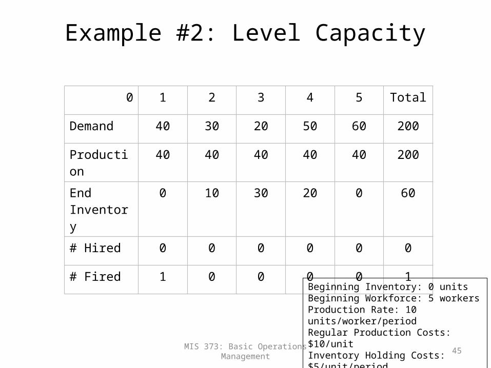
Example #2: Level Capacity
0 1 2 3 4 5 Total
Demand 40 30 20 50 60 200
Production 40 40 40 40 40 200
End Inventory
0 10 30 20 0 60
# Hired 0 0 0 0 0 0
# Fired 1 0 0 0 0 1
Beginning Inventory: 0 unitsBeginning Workforce: 5 workersProduction Rate: 10 units/worker/periodRegular Production Costs: $10/unitInventory Holding Costs: $5/unit/periodHiring Cost: $200/workerFiring Cost: $100/worker
MIS 373: Basic Operations Management
46
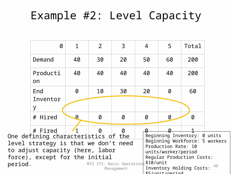
Example #2: Level Capacity
0 1 2 3 4 5 Total
Demand 40 30 20 50 60 200
Production 40 40 40 40 40 200
End Inventory
0 10 30 20 0 60
# Hired 0 0 0 0 0 0
# Fired 1 0 0 0 0 1
Beginning Inventory: 0 unitsBeginning Workforce: 5 workersProduction Rate: 10 units/worker/periodRegular Production Costs: $10/unitInventory Holding Costs: $5/unit/periodHiring Cost: $200/workerFiring Cost: $100/worker
One defining characteristics of the level strategy is that we don’t need to adjust capacity (here, labor force), except for the initial period.

MIS 373: Basic Operations Management
47
Example #2: Level Capacity
0 1 2 3 4 5 Total
Demand 40 30 20 50 60 200
Production 40 40 40 40 40 200
End Inventory
0 10 30 20 0 60
# Hired 0 0 0 0 0 0
# Fired 1 0 0 0 0 1
Beginning Inventory: 0 unitsBeginning Workforce: 5 workersProduction Rate: 10 units/worker/periodRegular Production Costs: $10/unitInventory Holding Costs: $5/unit/periodHiring Cost: $200/workerFiring Cost: $100/worker
TC=Production + Holding + Hiring + Firing
But, how to calculate the holding cost? Average inventory in a period
MIS 373: Basic Operations Management
48
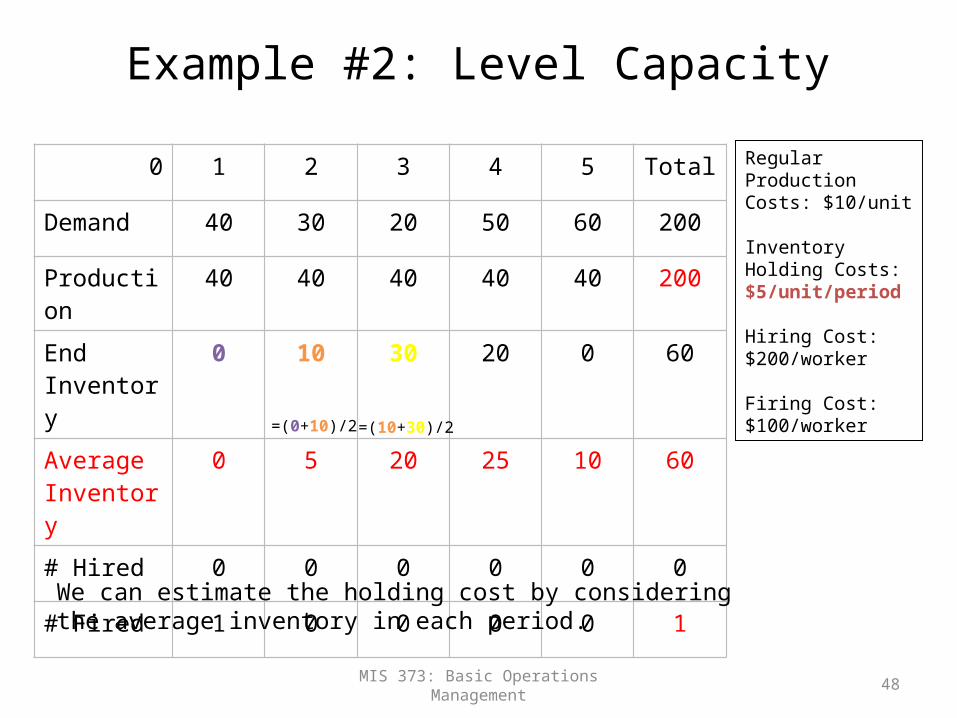
Example #2: Level Capacity
0 1 2 3 4 5 Total
Demand 40 30 20 50 60 200
Production 40 40 40 40 40 200
End Inventory
0 10 30 20 0 60
Average Inventory
0 5 20 25 10 60
# Hired 0 0 0 0 0 0
# Fired 1 0 0 0 0 1
We can estimate the holding cost by considering the average inventory in each period.
Regular Production Costs: $10/unit
Inventory Holding Costs: $5/unit/period
Hiring Cost: $200/worker
Firing Cost: $100/worker
=(0+10)/2 =(10+30)/2
MIS 373: Basic Operations Management
49
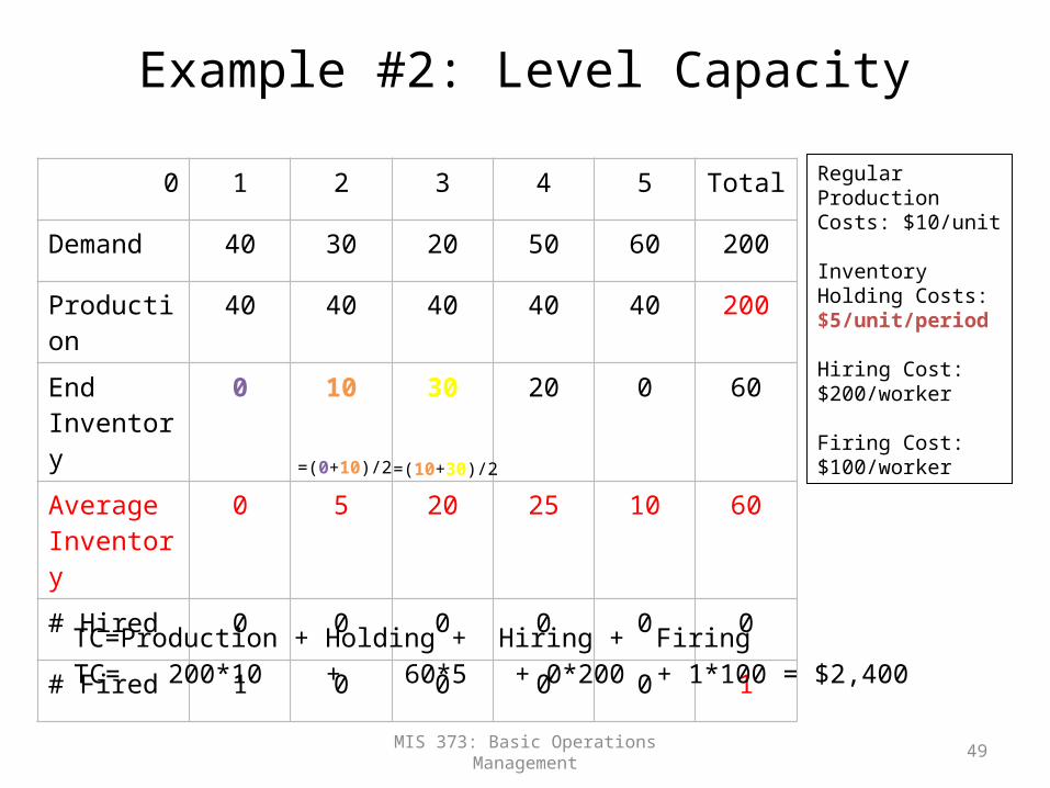
Example #2: Level Capacity
0 1 2 3 4 5 Total
Demand 40 30 20 50 60 200
Production 40 40 40 40 40 200
End Inventory
0 10 30 20 0 60
Average Inventory
0 5 20 25 10 60
# Hired 0 0 0 0 0 0
# Fired 1 0 0 0 0 1
TC= 200*10 + 60*5 + 0*200 + 1*100 = $2,400TC=Production + Holding + Hiring + Firing
Regular Production Costs: $10/unit
Inventory Holding Costs: $5/unit/period
Hiring Cost: $200/worker
Firing Cost: $100/worker
=(0+10)/2 =(10+30)/2
MIS 373: Basic Operations Management
50
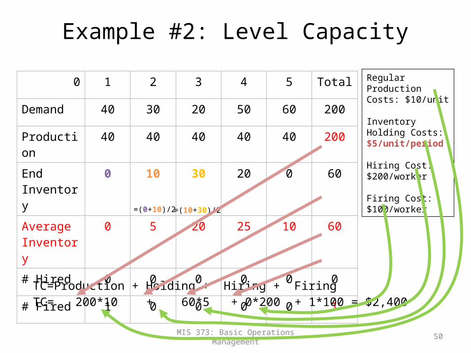
Example #2: Level Capacity
0 1 2 3 4 5 Total
Demand 40 30 20 50 60 200
Production 40 40 40 40 40 200
End Inventory
0 10 30 20 0 60
Average Inventory
0 5 20 25 10 60
# Hired 0 0 0 0 0 0
# Fired 1 0 0 0 0 1
TC= 200*10 + 60*5 + 0*200 + 1*100 = $2,400TC=Production + Holding + Hiring + Firing
Regular Production Costs: $10/unit
Inventory Holding Costs: $5/unit/period
Hiring Cost: $200/worker
Firing Cost: $100/worker
=(0+10)/2 =(10+30)/2

• Perform aggregate planning using the level strategy:• Beginning Inventory: 10 units• Beginning Workforce: 5 workers• Production Rate: 10 units/worker/period• Regular Production Costs: $10/unit• Inventory Costs: $10/unit/period• Hiring Cost: $100/worker• Firing Cost: $200/worker
Period 1 2 3 4 5Demand 50 40 30 30 40
Two additional assumptions: 1. Unmet demands in a period can be held and fulfilled in a future period.2. There is no cost associated with unmet demands.
Exercise

Beginning Inventory: 10 unitsBeginning Workforce: 5 workersProduction Rate: 10 units/worker/periodRegular Production Costs: $10/unitInventory Costs: $10/unit/periodHiring Cost: $100/workerFiring Cost: $200/worker
Beginning Inventory
10 1 2 3 4 5 Total
Demand 50 40 30 30 40 190
Production
End Inventory
Avg. Inventory
# Hired
# Fired
Solution
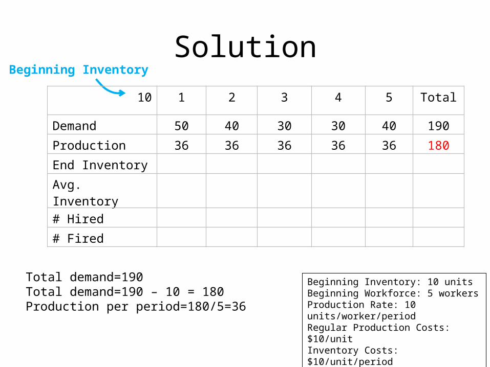
Beginning Inventory: 10 unitsBeginning Workforce: 5 workersProduction Rate: 10 units/worker/periodRegular Production Costs: $10/unitInventory Costs: $10/unit/periodHiring Cost: $100/workerFiring Cost: $200/worker
Beginning Inventory
Total demand=190Total demand=190 – 10 = 180Production per period=180/5=36
10 1 2 3 4 5 Total
Demand 50 40 30 30 40 190
Production 36 36 36 36 36 180
End Inventory
Avg. Inventory
# Hired
# Fired
Solution
Beginning Inventory: 10 unitsBeginning Workforce: 5 workersProduction Rate: 10 units/worker/periodRegular Production Costs: $10/unitInventory Costs: $10/unit/periodHiring Cost: $100/workerFiring Cost: $200/worker
Beginning Inventory
10 1 2 3 4 5 Total
Demand 50 40 30 30 40 190
Production 36 36 36 36 36 180
End Inventory -4
Avg. Inventory 3
# Hired 0
# Fired 1
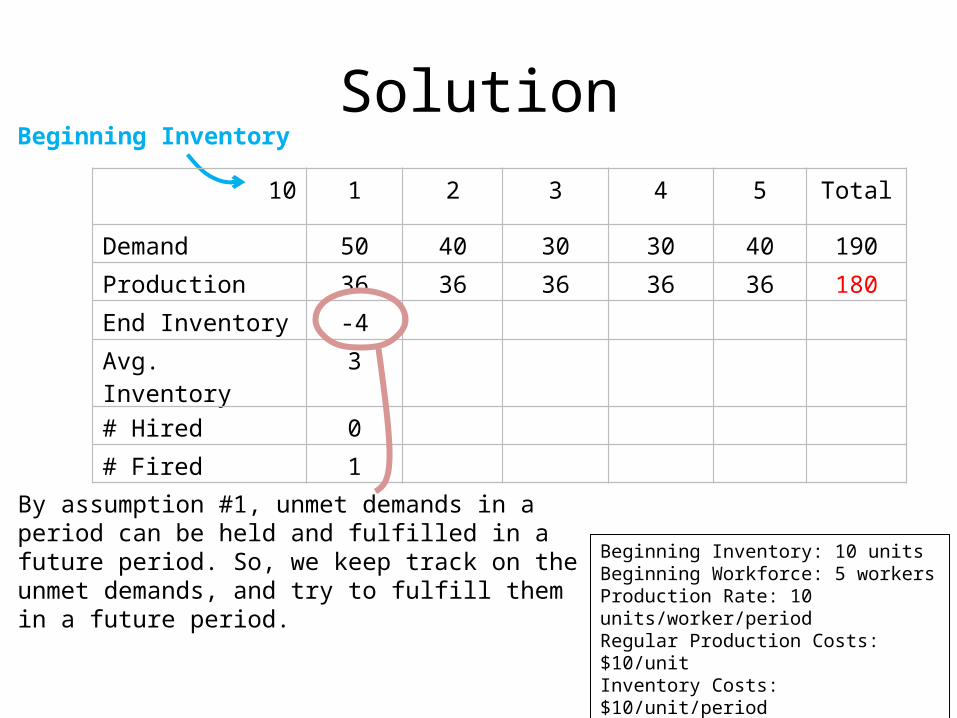
By assumption #1, unmet demands in a period can be held and fulfilled in a future period. So, we keep track on the unmet demands, and try to fulfill them in a future period.
Solution
Beginning Inventory: 10 unitsBeginning Workforce: 5 workersProduction Rate: 10 units/worker/periodRegular Production Costs: $10/unitInventory Costs: $10/unit/periodHiring Cost: $100/workerFiring Cost: $200/worker
Beginning Inventory
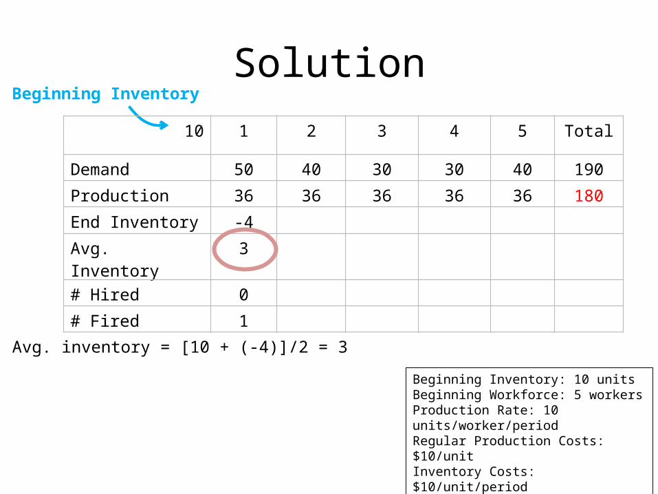
10 1 2 3 4 5 Total
Demand 50 40 30 30 40 190
Production 36 36 36 36 36 180
End Inventory -4
Avg. Inventory 3
# Hired 0
# Fired 1
Avg. inventory = [10 + (-4)]/2 = 3
Solution
Beginning Inventory: 10 unitsBeginning Workforce: 5 workersProduction Rate: 10 units/worker/periodRegular Production Costs: $10/unitInventory Costs: $10/unit/periodHiring Cost: $100/workerFiring Cost: $200/worker
Beginning Inventory
10 1 2 3 4 5 Total
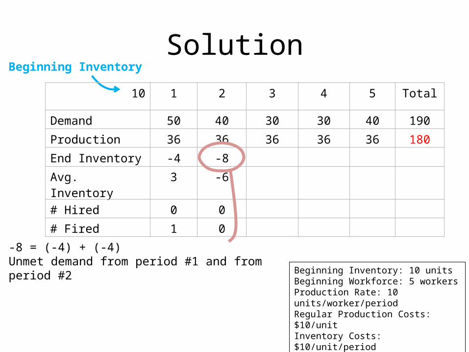
Demand 50 40 30 30 40 190
Production 36 36 36 36 36 180
End Inventory -4 -8
Avg. Inventory 3 -6
# Hired 0 0
# Fired 1 0
-8 = (-4) + (-4)Unmet demand from period #1 and from period #2
Solution
Beginning Inventory: 10 unitsBeginning Workforce: 5 workersProduction Rate: 10 units/worker/periodRegular Production Costs: $10/unitInventory Costs: $10/unit/periodHiring Cost: $100/workerFiring Cost: $200/worker
Beginning Inventory
10 1 2 3 4 5 Total
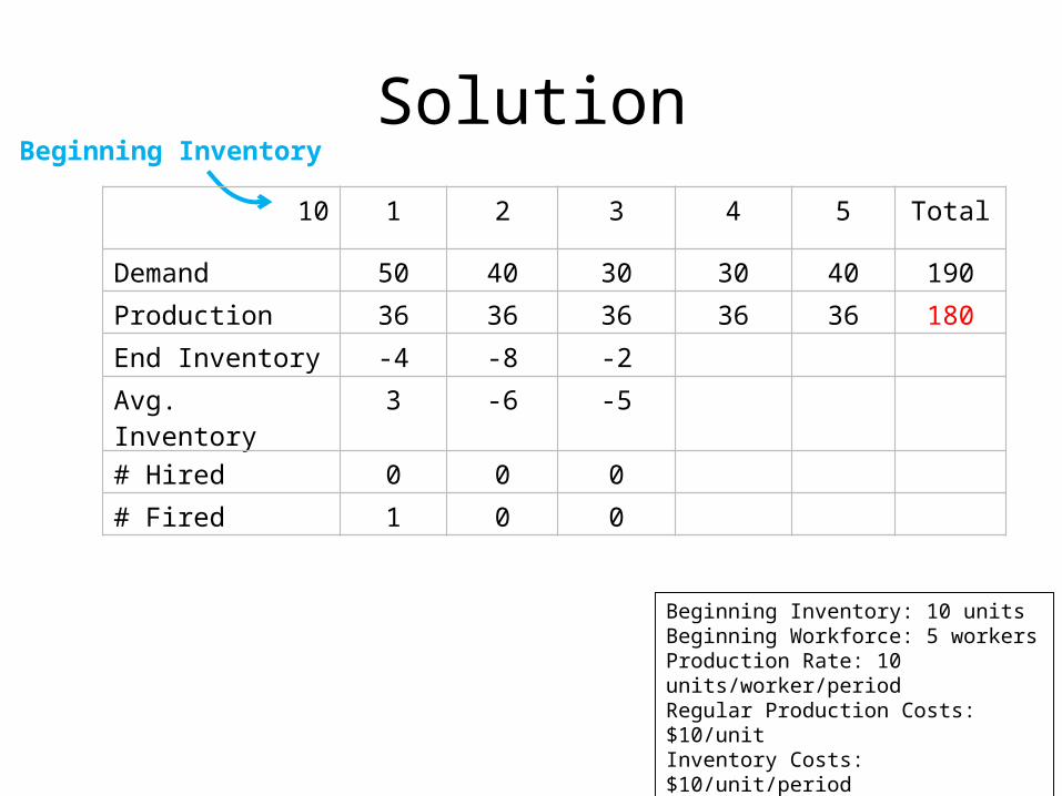
Demand 50 40 30 30 40 190
Production 36 36 36 36 36 180
End Inventory -4 -8 -2
Avg. Inventory 3 -6 -5
# Hired 0 0 0
# Fired 1 0 0
Solution
Beginning Inventory: 10 unitsBeginning Workforce: 5 workersProduction Rate: 10 units/worker/periodRegular Production Costs: $10/unitInventory Costs: $10/unit/periodHiring Cost: $100/workerFiring Cost: $200/worker
Beginning Inventory
10 1 2 3 4 5 Total
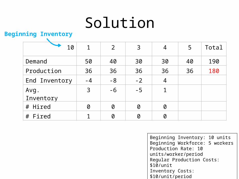
Demand 50 40 30 30 40 190
Production 36 36 36 36 36 180
End Inventory -4 -8 -2 4
Avg. Inventory 3 -6 -5 1
# Hired 0 0 0 0
# Fired 1 0 0 0
Solution
Beginning Inventory
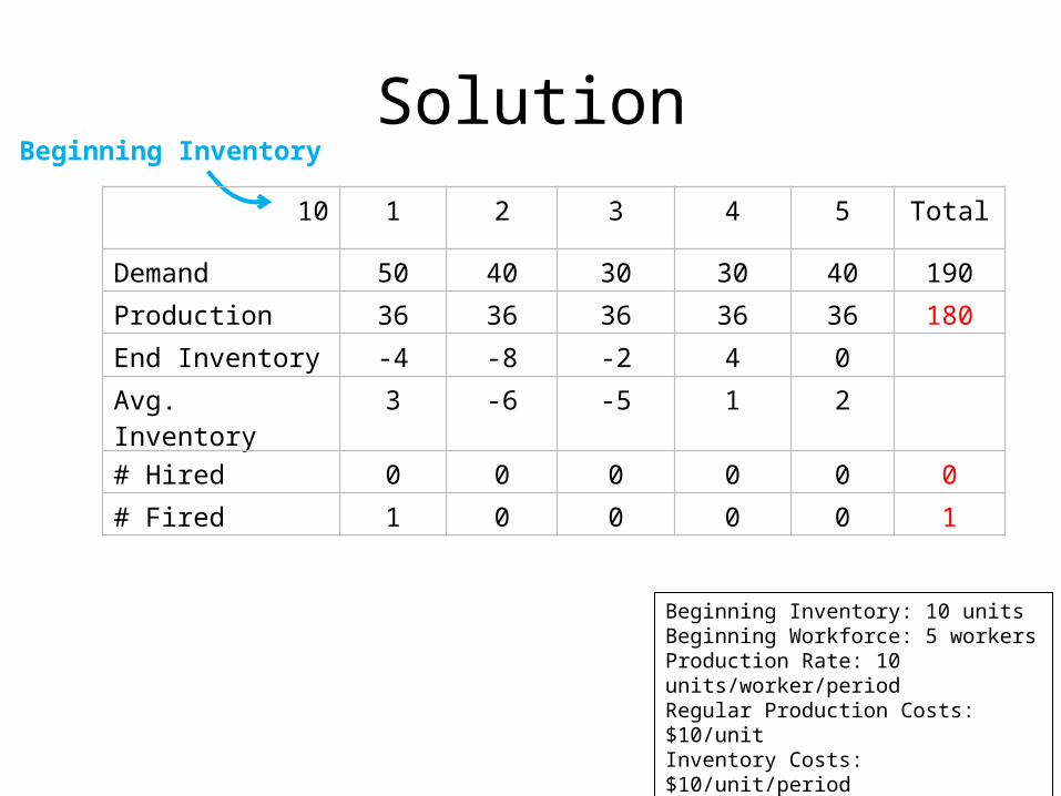
10 1 2 3 4 5 Total
Demand 50 40 30 30 40 190
Production 36 36 36 36 36 180
End Inventory -4 -8 -2 4 0
Avg. Inventory 3 -6 -5 1 2
# Hired 0 0 0 0 0 0
# Fired 1 0 0 0 0 1
Beginning Inventory: 10 unitsBeginning Workforce: 5 workersProduction Rate: 10 units/worker/periodRegular Production Costs: $10/unitInventory Costs: $10/unit/periodHiring Cost: $100/workerFiring Cost: $200/worker
Solution

Beginning Inventory: 10 unitsBeginning Workforce: 5 workersProduction Rate: 10 units/worker/periodRegular Production Costs: $10/unitInventory Costs: $10/unit/periodHiring Cost: $100/workerFiring Cost: $200/worker
Beginning Inventory
10 1 2 3 4 5 Total
Demand 50 40 30 30 40 190
Production 36 36 36 36 36 180
End Inventory -4 -8 -2 4 0
Avg. Inventory 3 -6 -5 1 2
# Hired 0 0 0 0 0 0
# Fired 1 0 0 0 0 1
By assumption #2, there is no cost associated with unmet demand (i.e., negative inventory has no costs).
TC=Production + Holding + Hiring + Firing = 180*10 + 10*(3+1+2) + 0 + 1*200 = $2,030
Solution
Negative Inventory has no meaning!
Beginning Inventory: 10 unitsBeginning Workforce: 5 workersProduction Rate: 10 units/worker/periodRegular Production Costs: $10/unitInventory Costs: $10/unit/periodHiring Cost: $100/workerFiring Cost: $200/worker
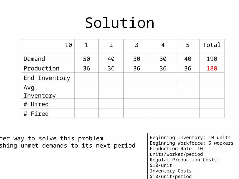
10 1 2 3 4 5 Total
Demand 50 40 30 30 40 190
Production 36 36 36 36 36 180
End Inventory
Avg. Inventory
# Hired
# Fired
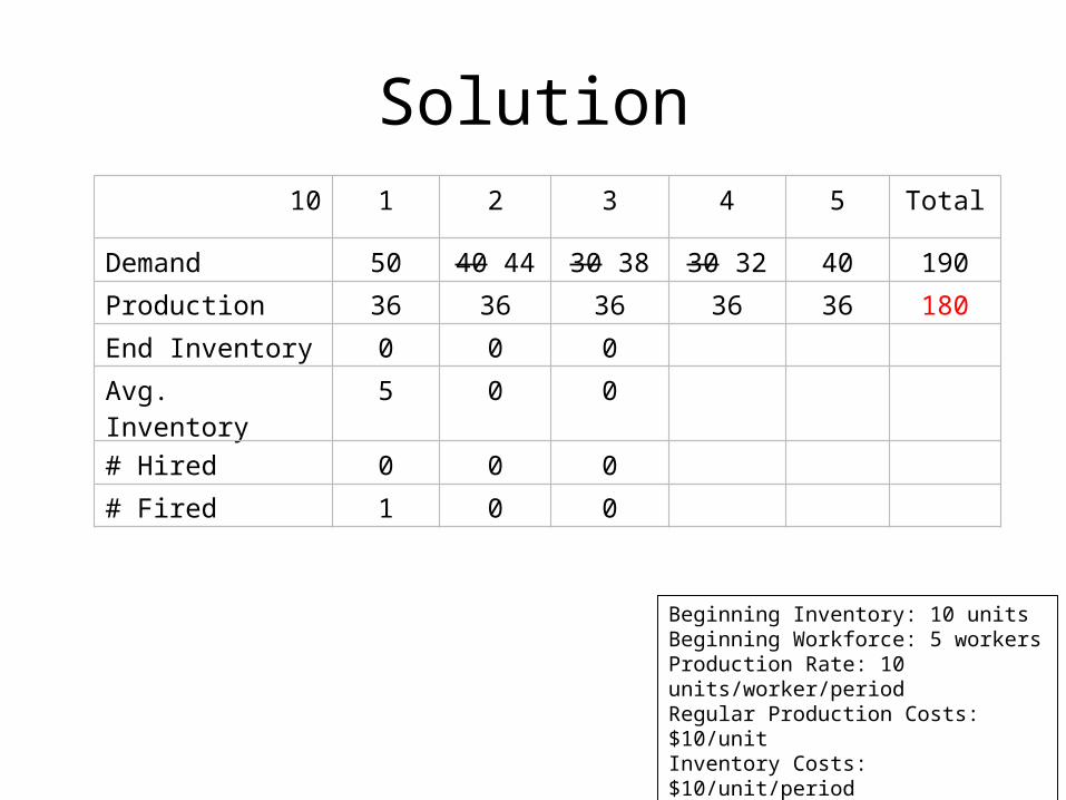
Another way to solve this problem. Pushing unmet demands to its next period
Solution
Beginning Inventory: 10 unitsBeginning Workforce: 5 workersProduction Rate: 10 units/worker/periodRegular Production Costs: $10/unitInventory Costs: $10/unit/periodHiring Cost: $100/workerFiring Cost: $200/worker
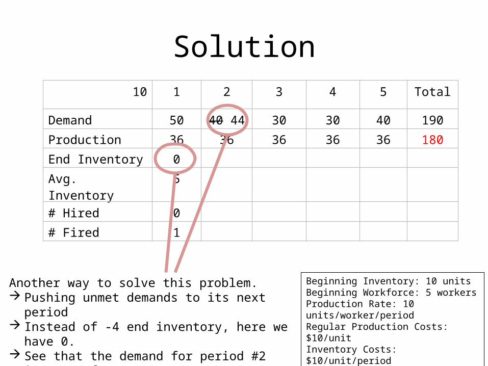
10 1 2 3 4 5 Total
Demand 50 40 44 30 30 40 190
Production 36 36 36 36 36 180
End Inventory 0
Avg. Inventory 5
# Hired 0
# Fired 1
Another way to solve this problem. Pushing unmet demands to its next period Instead of -4 end inventory, here we have 0. See that the demand for period #2 increase from 40 to
44.
Solution
Beginning Inventory: 10 unitsBeginning Workforce: 5 workersProduction Rate: 10 units/worker/periodRegular Production Costs: $10/unitInventory Costs: $10/unit/periodHiring Cost: $100/workerFiring Cost: $200/worker
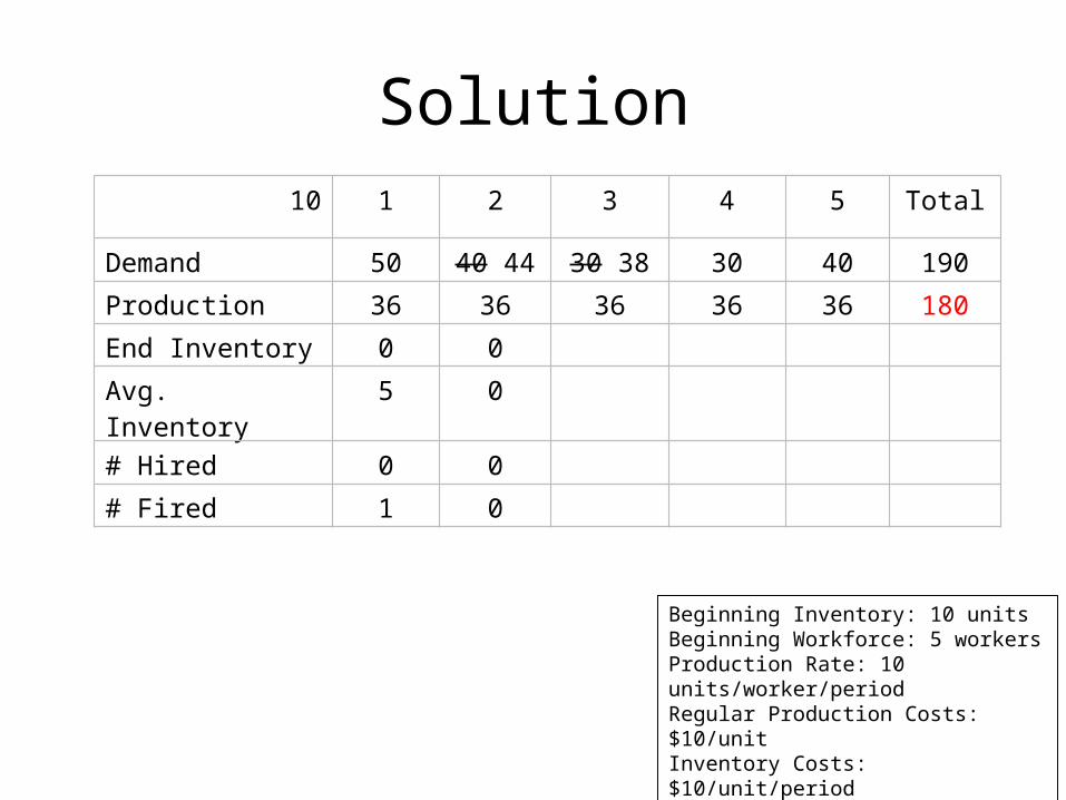
10 1 2 3 4 5 Total
Demand 50 40 44 30 38 30 40 190
Production 36 36 36 36 36 180
End Inventory 0 0
Avg. Inventory 5 0
# Hired 0 0
# Fired 1 0
Solution
Beginning Inventory: 10 unitsBeginning Workforce: 5 workersProduction Rate: 10 units/worker/periodRegular Production Costs: $10/unitInventory Costs: $10/unit/periodHiring Cost: $100/workerFiring Cost: $200/worker
10 1 2 3 4 5 Total
Demand 50 40 44 30 38 30 32 40 190
Production 36 36 36 36 36 180
End Inventory 0 0 0
Avg. Inventory 5 0 0
# Hired 0 0 0
# Fired 1 0 0
Solution

Beginning Inventory: 10 unitsBeginning Workforce: 5 workersProduction Rate: 10 units/worker/periodRegular Production Costs: $10/unitInventory Costs: $10/unit/periodHiring Cost: $100/workerFiring Cost: $200/worker
10 1 2 3 4 5 Total
Demand 50 40 44 30 38 30 32 40 190
Production 36 36 36 36 36 180
End Inventory 0 0 0 4
Avg. Inventory 5 0 0 2
# Hired 0 0 0 0
# Fired 1 0 0 0
Solution
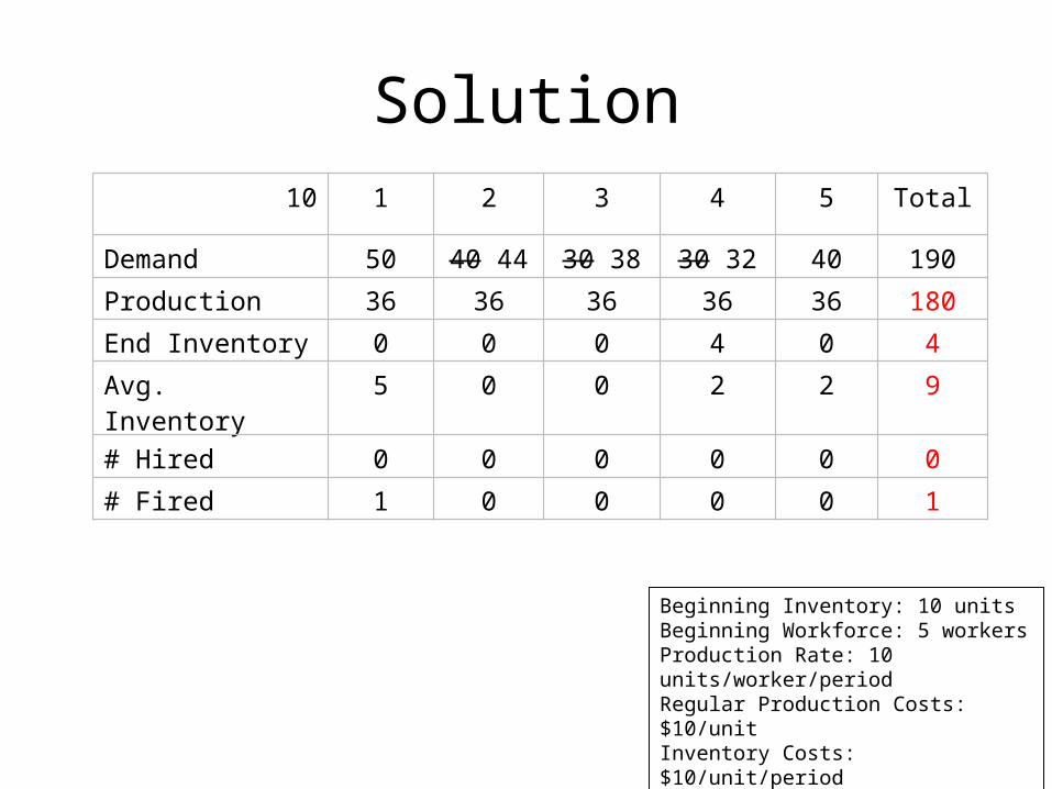
Beginning Inventory: 10 unitsBeginning Workforce: 5 workersProduction Rate: 10 units/worker/periodRegular Production Costs: $10/unitInventory Costs: $10/unit/periodHiring Cost: $100/workerFiring Cost: $200/worker
10 1 2 3 4 5 Total
Demand 50 40 44 30 38 30 32 40 190
Production 36 36 36 36 36 180
End Inventory 0 0 0 4 0 4
Avg. Inventory 5 0 0 2 2 9
# Hired 0 0 0 0 0 0
# Fired 1 0 0 0 0 1
Solution
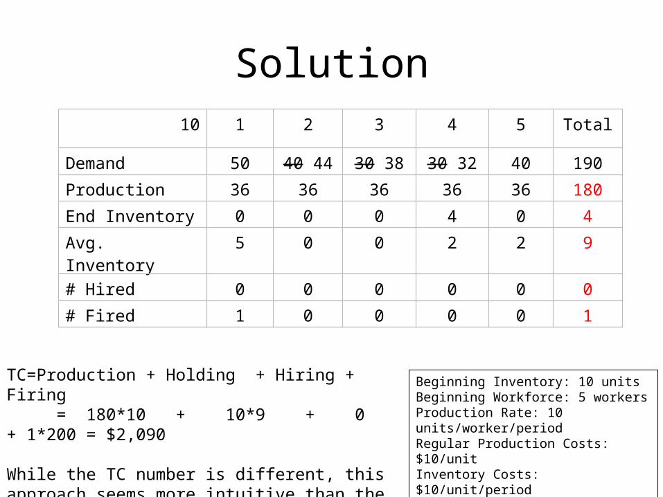
Beginning Inventory: 10 unitsBeginning Workforce: 5 workersProduction Rate: 10 units/worker/periodRegular Production Costs: $10/unitInventory Costs: $10/unit/periodHiring Cost: $100/workerFiring Cost: $200/worker
10 1 2 3 4 5 Total
Demand 50 40 44 30 38 30 32 40 190
Production 36 36 36 36 36 180
End Inventory 0 0 0 4 0 4
Avg. Inventory 5 0 0 2 2 9
# Hired 0 0 0 0 0 0
# Fired 1 0 0 0 0 1
TC=Production + Holding + Hiring + Firing = 180*10 + 10*9 + 0 + 1*200 = $2,090
While the TC number is different, this approach seems more intuitive than the previous approach, especially on the parts about inventory.
Solution
MIS 373: Basic Operations Management
68
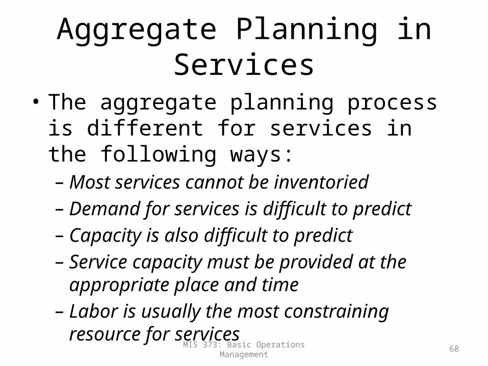
Aggregate Planning in Services
• The aggregate planning process is different for services in the following ways: – Most services cannot be inventoried– Demand for services is difficult to predict– Capacity is also difficult to predict– Service capacity must be provided at the
appropriate place and time– Labor is usually the most constraining resource for
services
MIS 373: Basic Operations Management
69
Aggregate Planning in Services
• Hospitals:– allocate funds, staff, and supplies to meet the demands of patients
for their medical services• Restaurants:
– smoothing the service rate, determining workforce size, and managing demand to match a fixed capacity
– Perishable inventory• Airlines:
– complex due to the large number of factors involved (planes, flight & group personnel, multiple routes, airports etc.)
– Capacity decisions must also take into account the percentage of seats to be allocated to various fare classes in order to maximize profit or yield (Revenue Management)


![[PPT]Production and Operations Management: …sureten/(aggregate planning)5.ppt · Web viewDisaggregating the Aggregate Plan Aggregate Planning Aggregate planning Intermediate-range](https://static.documents.pub/doc/80x56/5aec86827f8b9ab24d902697/pptproduction-and-operations-management-suretenaggregate-planning5pptweb.jpg)


