Aggregate Risk and the Choice between Cash and Lines of Credit

THE JOURNAL OF FINANCE • VOL. LXVIII, NO. 5 • OCTOBER 2013

Aggregate Risk and the Choice between Cashand Lines of Credit

VIRAL V. ACHARYA, HEITOR ALMEIDA, and MURILLO CAMPELLO∗

ABSTRACT

Banks can create liquidity for firms by pooling their idiosyncratic risks. As a result,bank lines of credit to firms with greater aggregate risk should be costlier and suchfirms opt for cash in spite of the incurred liquidity premium. We find empirical sup-port for this novel theoretical insight. Firms with higher beta have a higher ratio ofcash to credit lines and face greater costs on their lines. In times of heightened ag-gregate volatility, banks exposed to undrawn credit lines become riskier; bank creditlines feature fewer initiations, higher spreads, and shorter maturity; and, firms’ cashreserves rise.

A FEDERAL RESERVE SURVEY earlier this year found that about one-third ofU.S. banks have tightened their standards on loans they make to busi-nesses of all sizes. And about 45% of banks told the Fed that they arecharging more for credit lines to large and midsize companies. Bankssuch as Citigroup Inc., which has been battered by billions of dollars inwrite-downs and other losses, are especially likely to play hardball, re-sisting pleas for more credit or pushing borrowers to pay more for loanmodifications.

—The Wall Street Journal, March 8, 2008

How do firms manage their liquidity needs? This question has become in-creasingly important for both academic research and corporate finance in prac-tice. Survey evidence indicates that liquidity management tools such as cashand credit lines are essential components of a firm’s financial policy (see Lins,

∗Viral V. Acharya is with NYU–Stern, CEPR, ECGI, and NBER. Heitor Almeida is with Uni-versity of Illinois and NBER. Murillo Campello is with Cornell University and NBER. Our paperbenefited from comments from Peter Tufano (Acting Editor); an anonymous referee; Hui Chen,Ran Duchin, and Robert McDonald (discussants); Rene Stulz; as well as seminar participants atthe 2010 AEA meetings, 2010 WFA meetings, DePaul University, ESSEC, Emory University, MIT,Moody’s/NYU–Stern 2010 Credit Risk Conference, New York University, Northwestern University,UCLA, University of Illinois, Vienna University of Economics and Business, Yale University, Uni-versity of Southern California, and UCSD. We thank Florin Vasvari and Anurag Gupta for helpwith the data on lines of credit, and Michael Roberts and Florin Vasvari for matching these datawith COMPUSTAT. Farhang Farazmand, Fabrıcio D’Almeida, Igor Cunha, Rustom Irani, HanhLe, Ping Liu, and Quoc Nguyen provided excellent research assistance. We are also grateful toJaewon Choi for sharing his data on firm betas, and to Thomas Philippon and Ran Duchin forsharing their programs to compute asset and financing gap betas.

DOI: 10.1111/jofi.12056

2059

2060 The Journal of Finance R©

Servaes, and Tufano (2010), Campello et al. (2011)). Consistent with the evi-dence from surveys, a number of studies show that the funding of investmentopportunities is a key determinant of corporate cash policy (e.g., Opler et al.(1999), Almeida, Campello, and Weisbach (2004, 2009), and Duchin (2009)).Recent work also shows that bank lines of credit have become an importantsource of firm financing (Sufi (2009), Disatnik, Duchin, and Schmidt (2010)).The evidence further suggests that credit lines played a crucial role in theliquidity management of firms during the recent credit crisis (Ivashina andScharfstein (2010)).

In contrast to the growing empirical literature, there is limited theoreticalwork on the reasons why firms may use “pre-committed” sources of funds (suchas cash or credit lines) to manage their liquidity needs. In principle, a firm canuse other sources of funding for long-term liquidity management, such as futureoperating cash flows or proceeds from debt issuances. However, these alterna-tives expose the firm to additional risks because their availability depends onfirm performance. Holmstrom and Tirole (1997, 1998), for example, show thatrelying on future issuance of external claims is insufficient to provide liquidityfor firms that face costly external financing. Similarly, Acharya, Almeida, andCampello (2007) show that cash holdings dominate spare debt capacity for fi-nancially constrained firms whose financing needs are concentrated in statesof the world in which cash flows are low. Notably, these models of liquidityinsurance are silent on the trade-offs between cash and credit lines.1

This paper attempts to fill this gap in the liquidity management literature.Building on Holmstrom and Tirole (1998) and Tirole (2006), we develop a modelof the trade-offs firms face when choosing between holding cash and securinga credit line. The key insight of our argument is that a firm’s exposure toaggregate risks—its “beta”—is a fundamental determinant of liquidity choices.The intuition is straightforward. In the presence of a liquidity premium (e.g., alow return on cash holdings), firms find it costly to hold cash. Firms may insteadmanage their liquidity needs using bank credit lines, which do not require themto hold liquid assets. Under a credit line agreement, the bank provides the firmwith funds when the firm faces a liquidity shortfall. In exchange, the bankcollects payments from the firm in states of the world in which the firm doesnot need the funds under the line (e.g., commitment fees). The credit line canthus be seen as an insurance contract. Provided that the bank can offer thisinsurance at “actuarially fair” terms, lines of credit will dominate cash holdingsin corporate liquidity management.

The drawback of credit lines, however, is that banks may not be able toprovide liquidity insurance for all firms in the economy at all times. Consider,for example, a situation in which a large fraction of the corporate sector is hit bya liquidity shock. In this state of the world, banks might be unable to guarantee

1 A recent paper by Bolton, Chen, and Wang (2011) introduces both cash and credit lines in adynamic investment framework with costly external finance. In their model, the size of the creditline facility is given exogenously, and thus they do not analyze the ex-ante trade-off between cashand credit lines (see also DeMarzo and Fishman (2007)).

Aggregate Risk and the Choice between Cash and Lines of Credit 2061

liquidity since the demand for funds under the outstanding lines (drawdowns)may exceed the supply of funds coming from healthy firms. In other words, theability of the banking sector to meet corporate liquidity needs depends on theextent to which firms are subject to correlated (systematic) liquidity shocks.Aggregate risk thus creates a cost to credit lines.

We explore this trade-off between aggregate risk and liquidity premia toderive optimal corporate liquidity policy. We do so in an equilibrium modelin which firms are heterogeneous with respect to their exposure to aggregaterisks (firms have different betas). We show that, while low beta firms managetheir liquidity through bank credit lines, high beta firms optimally choose tohold cash, despite the liquidity premium. Because the banking sector managesprimarily idiosyncratic risk, it can provide liquidity for low beta firms evenin bad states of the world. In equilibrium, low beta firms therefore face bettercontractual terms when initiating credit lines, demand more lines, and hold lesscash in equilibrium. On the flip side, high beta firms face worse contractualterms, demand fewer lines, and hold more cash. This logic suggests that firms’exposure to systematic risks increases the demand for cash and reduces thedemand for credit lines. In a similar fashion, when there is an increase inaggregate risk there is greater aggregate reliance on cash relative to creditlines.

In addition to this basic result, the model generates a number of insights onliquidity management. These, in turn, motivate our empirical analysis. First,the model suggests that exposure to risks that are systematic to the bankingindustry should affect corporate liquidity policy. In particular, firms that aremore sensitive to banking industry downturns should be more likely to holdcash for liquidity management. Second, the trade-off between cash and creditlines should be more important for firms that find it more costly to raise externalcapital. Third, the effect of aggregate risk exposure on liquidity policy shouldbe stronger for firms that have high aggregate risk, as these firms have thestrongest impact on bank liquidity constraints. Fourth, lines of credit shouldbe more expensive for firms with greater aggregate risk and in times of higheraggregate volatility.

We test these cross-sectional and time-series implications using data from the1987 to 2008 period.2 For the cross-sectional analysis, we use two alternativedata sources to construct proxies for the availability of credit lines. Our firstsample is drawn from the LPC-DealScan database. These data allow us toconstruct a large sample of credit line initiations. The LPC-DealScan data,however, have two limitations. First, they are based largely on syndicated loans,and thus biased toward large deals (and consequently large firms). Second, theydo not reveal the extent to which existing lines have been used (drawdowns).To overcome these issues, we also use an alternative sample that containsdetailed information on the credit lines initiated and used by a random sample

2 To be precise, we use a panel data set to test the model’s cross-sectional implications. However,most of the variation in our proxies for firm-level systematic risk exposure is cross-sectional innature.


of 300 firms between 1996 and 2003. These data are drawn from Sufi (2009).Using both LPC-DealScan and Sufi’s data sets, we measure the fraction ofcorporate liquidity that is provided by lines of credit as the ratio of total creditlines to the sum of total credit lines plus cash. We call this variable the LC-to-Cash ratio. While some firms may have higher demand for total liquiditydue to variables such as better investment opportunities, the LC-to-Cash ratioisolates the relative use of lines of credit versus cash in corporate liquiditymanagement.

Our main hypothesis is that a firm’s exposure to aggregate risk should benegatively related to its LC-to-Cash ratio. In the model, the relevant aggregaterisk is the correlation of a firm’s financing needs with those of other firms inthe economy. While this could suggest using a “cash flow beta,” note that cashflow-based measures are slow-moving and available only at a low frequency.Under the assumption that a firm’s financing needs go up when its stock returnfalls, the relevant beta is the traditional beta of the firm with respect to theoverall stock market. Accordingly, we employ a standard stock market-basedbeta as our baseline measure of risk exposure. For robustness, however, wealso use cash flow-based betas.3 To test the prediction that a firm’s exposureto banking sector risk should influence the firm’s liquidity policy, we measure“bank beta” as the beta of a firm’s returns with respect to the banking sector’saggregate return.

Our market-based measures of beta are asset (i.e., unlevered) betas. Whileequity betas are easy to compute using stock price data, they are mechani-cally related to leverage (high leverage firms tend to have larger betas). Sincegreater reliance on credit lines will typically increase the firm’s leverage, the“mechanical” leverage effect may bias our estimates. To overcome this problem,we unlever equity betas by using a Merton-KMV-type model for firm value, oralternatively we compute betas using data on firm asset returns (from Choi(2009)). We also tease out the relative importance of systematic and idiosyn-cratic risk for corporate liquidity policy by decomposing total asset risk into itssystematic and idiosyncratic components.

We test the theory’s cross-sectional implications by relating systematic riskexposure to LC-to-Cash ratios. In a nutshell, all of our tests lead to a similarconclusion: exposure to systematic risk has a statistically and economicallysignificant impact on the fraction of corporate liquidity that is provided by creditlines. Using the LPC-DealScan sample, for example, we find that an increase inbeta from 0.8 to 1.5 (this is less than a one-standard-deviation change in beta)decreases a firm’s reliance on credit lines by 0.06 (approximately 15% of thestandard deviation and 20% of the sample average value of LC-to-Cash). Wealso find that the systematic component of asset variance has a negative andsignificant effect on the LC-to-Cash ratio. These findings support our theory’s

3 In addition, we employ a “tail beta” that uses data from the days with the worst returns in theyear to compute beta (see Acharya et al. (2010)). This beta proxy captures the idea that a firm’sexposure to systematic risks matters mostly on the downside (because a firm may need liquiditywhen other firms face problems).


predictions. Notably, the inferences we draw hold across both the larger LPC-DealScan data set and the smaller, more detailed data constructed by Sufi (bothfor total and unused credit lines).

The negative relation between systematic risk exposure and LC-to-Cashholds for all the beta proxies that we employ, including Choi’s (2009) assetreturn-based betas, betas that are unlevered using net rather than gross debt(to account for a possible effect of cash on asset betas), equity (levered) betas,and cash flow-based betas. The results also hold for “bank betas” (suggest-ing that firms that are more sensitive to banking industry downturns are morelikely to hold cash for liquidity management) and “tail betas” (suggesting that afirm’s sensitivity to market downturns affects corporate liquidity policy). Theseestimates agree with our theory and imply a strong economic relation betweenexposure to aggregate risk and liquidity management.

In additional tests, we sort firms according to observable proxies of financingconstraints to study whether the effect of beta on LC-to-Cash is driven byfirms that are likely to be constrained. As predicted by our model, the relationbetween beta and the use of credit lines only holds in samples of firms likely tobe constrained (e.g., small and low payout firms). When we sort firms into “highbeta” and “low beta” groups, we find that the effect of beta on the LC-to-Cashratio is significantly stronger in the sample of high beta firms (consistent withour story). Finally, we study the relation between firms’ beta and the fees andspreads that they commit to pay on bank lines of credit. We find that high betafirms pay significantly higher fees on their undrawn balances, and also higherspreads when drawing on their credit lines. This is direct evidence that it ismore costly for banks to provide liquidity insurance for aggregate-risky firms.

Next, we examine our model’s time-series implications. These tests gaugeaggregate risk using VIX, the implied volatility of the stock market indexreturns from options data. This variable captures both aggregate volatility aswell as the financial sector’s appetite to bear that risk. In addition, we examinewhether expected volatility in the banking sector drives time-series variationin corporate liquidity policy. Given limited historical data on implied volatilityfor the banking sector, we construct Bank VIX, the expected banking sectorvolatility, using a GARCH model.

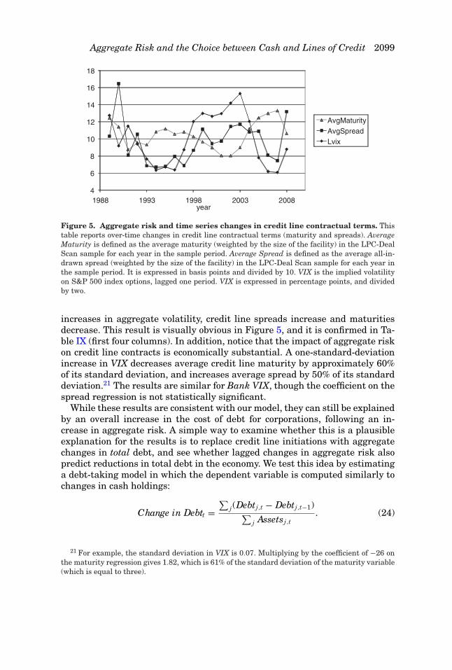
Controlling for real GDP growth and flight-to-quality effects (see Gatev andStrahan (2006)), we find that an increase in VIX and/or Bank VIX reducescredit line initiations and raises firms’ cash reserves (Figure 4 provides a visualillustration). The maturity of credit lines shrinks as aggregate volatility rises,and new credit lines become more expensive in those times (see Figure 5). Weconfirm that these effects are not due to an overall increase in the cost of debtby showing that firms’ debt issuances are not affected by VIX. In other words,the negative impact of VIX on new debt operates through availability of lines ofcredit. These results suggest that an increase in aggregate risk in the economyis an important limitation of bank-provided liquidity insurance to firms.

Finally, we provide evidence for the mechanism that drives corporate liq-uidity choices in our model. The model suggests that an increase in aggre-gate risk in the economy creates liquidity risk for banks that are exposed to


undrawn corporate credit lines. Thus, banks increase the cost of credit lines foraggregate-risky firms, which in turn move toward cash holdings. Nevertheless,a possible alternative interpretation for the results is related to the risk ofcovenant violations (as in Sufi (2009)). For example, if firms are more likely toviolate covenants in times when aggregate risk is high, then high beta firmsmay move to cash holdings not because of banks’ liquidity constraint as in ourmodel, but because of the risk of covenant violations.

To disentangle these two stories, we employ a direct test of the predictionthat aggregate risk exposure tightens banks’ liquidity constraints through acredit line channel. Gatev, Schuermann, and Strahan (2009) study the link be-tween credit line exposure and bank risk, and find that bank risk, as measuredby stock return volatility, increases with unused credit lines that the bankhas agreed to extend to the corporate sector. The mechanism in our modelwould then suggest that the impact of credit line exposure on bank risk shouldincrease during periods of high aggregate risk. We test and confirm this predic-tion using bank-level data (taken from Call Reports). In addition, we examinethe hypothesis that covenant violations (or credit line revocations conditionalon violations) increase during periods of high aggregate volatility (or for firmswith high aggregate risk exposure). Our results suggest that aggregate riskdoes not increase the sensitivity of covenant violations to profitability shocks.In addition, the effect of covenant violations on credit line revocations is largelyindependent of firms’ aggregate risk exposures.4 These results provide addi-tional evidence that the link between liquidity management and aggregate riskuncovered in our tests is indeed due to the effect of aggregate risk on banks’liquidity constraints.

Our work has connections with recent literature that discusses firms’ liquid-ity choices and it is important that we highlight our contributions. Comparedto Sufi (2009), our contribution is to show that the (largely idiosyncratic) riskof covenant violations is not the only type of risk that affects firms’ choice be-tween cash and credit lines. Firms’ exposure to aggregate risk, and the ensuingeffects on banks’ liquidity constraints, are also key forces that drive corporateliquidity policy. Compared to the growing literature on firms’ choices betweencredit lines and cash (e.g., Lins, Servaes, and Tufano (2010), Campello et al.(2011), and Disatnik, Duchin, and Schmidt (2010)), we are the first to advanceand test a full-fledged theory explaining how corporate exposure to aggregaterisk drives firms’ liquidity management. We also provide a novel assessmentof the importance of financial intermediary risk for the choice between cashand credit lines. In fact, papers on the cash–credit line choice generally ab-stract from connections between the macroeconomy, banks, and firms when

4 Since a credit line is a loan commitment, it may not be easy for the bank to revoke access tothe line once it is initiated. In order for the bank to revoke access, the firm must be in violation of acovenant. Given that covenant violations are unrelated to systematic risk after controlling for firmprofitability (as the evidence in this paper suggests), banks do not revoke access simply becauseaggregate risk is high.


examining liquidity management.5 We believe our paper represents a step for-ward in establishing a theoretical framework describing these connections andin showing how they operate. Understanding and characterizing these linksshould be of interest for future research, especially around important episodessuch as financial crises.

The paper is organized as follows. In Section I, we develop our model andderive its empirical implications. We present the empirical tests in Section II.Section III offers concluding remarks.

I. Model

Our model is based on Holmstrom and Tirole (1998) and Tirole (2006), whoconsider the role of aggregate risk in affecting corporate liquidity policy. Weintroduce firm heterogeneity to their framework to analyze the trade-offs be-tween cash and credit lines.

The economy has a unit mass of firms. Each firm has access to an investmentproject that requires fixed investment I at date 0. The investment opportunityalso requires an additional investment at date 1 of uncertain size. This addi-tional investment represents the firms’ liquidity need at date 1. We assume thatthe date-1 investment need can be equal to either ρ, with probability λ, or zero,with probability (1 − λ). There is no discounting and everyone is risk-neutral,so that the discount factor is one.

Firms are symmetric in all aspects, with one important exception. They differin the extent to which their liquidity shocks are correlated with each other.A fraction θ of firms has perfectly correlated liquidity shocks; that is, eitherthese firms have a date-1 investment need or they do not. We call these firmssystematic firms. The other fraction of firms (1 − θ ) has independent investmentneeds; that is, the probability that a firm needs ρ is independent of whetherother firms need ρ or zero. These are nonsystematic firms. We can think of thissetup as one in which an aggregate state realizes first. The realized state thendetermines whether systematic firms have liquidity shocks.

We refer to states as follows. We let the aggregate state in which systematicfirms have a liquidity shock be denoted by λθ . Similarly, (1 − λθ ) is the state inwhich systematic firms have no liquidity demand. After the realization of thisaggregate state, nonsystematic firms learn whether they have liquidity shocks.The state in which nonsystematic firms do get a shock is denoted as λ and theother state as (1 − λ). Note that the likelihood of both λ and λθ states is λ. Inother words, to avoid additional notation, we denote states by their probability,but single out the state in which systematic firms are all hit by a liquidity shockwith the superscript θ . The setup is summarized in Figure 1.

A firm will only continue its date-0 investment until date 2 if it can meetits date-1 liquidity need. If the liquidity need is not met, the firm is liquidatedand the project produces a cash flow equal to zero. If the firm continues, the

5 Exceptions are papers written on the 2008 to 2009 crisis, such as Campello et al. (2011) andIvashina and Scharfstein (2010).


0t =

I

θλ−1

θλ

1 λ−

1 λ−

λ

λ

0ρ =1t =

0ρ >

0ρ =

0ρ >0ρ >

0ρ =

Systematic shock to fraction θ of firms

Idiosyncratic shock to other firms

2t =Continuationsubject to moral hazard

Continuationsubject to moral hazard

Liquidations

Liquidations

Figure 1. Timeline of the model.

investment produces a date-2 cash flow R that obtains with probability p.With probability 1 − p, the investment produces nothing. The probability ofsuccess depends on the input of specific human capital by the firms’ managers.If the managers exert high effort, the probability of success is equal to pG.Otherwise, the probability is pB, but the managers consume a private benefitequal to B. While the cash flow R is verifiable, managerial effort and the privatebenefit are not verifiable and contractible. Because of the moral hazard due thisprivate benefit, managers must keep a high enough stake in the project to beinduced to exert effort. We assume that the investment is negative NPV ifthe managers do not exert effort, implying the following incentive constraint:pGRM ≥ pBRM + B, or RM ≥ B

�p , where RM is managers’ compensation and�p = pG − pB. This moral hazard problem implies that the firms’ cash flowscannot be pledged in their entirety to outside investors. Following Holmstromand Tirole (1998), we define

ρ0 ≡ pG

(R − B

�p

)< ρ1 ≡ pGR. (1)

The parameter ρ0 represents the investment’s pledgable income, and ρ1 itstotal expected payoff.

In addition, we assume that the project can be partially liquidated at date 1.Specifically, a firm can choose to continue only a fraction x < 1 of its investmentproject, in which case (in its liquidity shock state, λ or λθ ) it requires a date-1investment of xρ. It then produces total expected cash flow equal to xρ1 andpledgable income equal to xρ0. In other words, the project can be linearly scaleddown at date 1. We make the following assumption:

ρ0 < ρ < ρ1. (2)


The assumption that ρ < ρ1 implies that the efficient level of x is xFB = 1.However, the firm’s pledgable income is lower than the liquidity shock. Thismight force the firm to liquidate some of its projects and thus have x∗ < 1in equilibrium. For each x, it can raise xρ0 in the market at date 1. As inHolmstrom and Tirole, we assume that the firm can fully dilute the date-0investors at date 1, that is, the firm can issue securities that are senior to thedate-0 claim to finance a part of the required investment xρ (alternatively, wecan assume efficient renegotiation of the date-0 claim).

Finally, we assume that, even when x = 1, each project produces enoughpledgable income to finance the initial investment I and the date-1 invest-ment ρ:

I < (1 − λ)ρ0 + λ(ρ0 − ρ). (3)

In particular, notice that this implies that (1 − λ)ρ0 > λ(ρ − ρ0).

A. The Role of Liquidity Management

Before we characterize the optimal solution using credit lines and cash, itis worth exploring the common feature to both of them, which is their role asprecommitted financing. This discussion also clarifies why alternative strate-gies such as excess debt capacity are imperfect substitutes for precommittedfinancing through cash or credit lines.

In order to see this, consider what happens to the firm when it carries no cashand no credit line, but saves maximum future debt capacity by borrowing aslittle as it can today (that is, exactly I). The firm plans to borrow on the spot debtmarket at date 1, once the liquidity shock materializes (in state λ). Given theassumptions above, this debt capacity strategy is bound to fail. Even underthe assumption of full dilution of date-0 investors, the maximum amount thatthe firm can borrow in the spot market at date 1 for a given x is xρ0. But sincexρ0 < xρ for all x, the firm does not have enough funds to pay for the liquidityshock and hence must liquidate the project. In other words, in the absence ofcash and/or a credit line, x∗ = 0.

The problem with this “wait and see” strategy is that it does not generateenough debt capacity in future liquidity states, while at the same time wastingdebt capacity in states of the world with no liquidity shock. Notice that, in theno-liquidity-shock state (state 1 − λ), the firm has debt capacity equal to ρ0 butno required investments. In this context, the role of corporate liquidity policy(that is, cash and credit lines) is to transfer financing capacity from the good tothe bad state of the world. The firm accomplishes this transfer using cash byborrowing more than I at date 0, and promising a larger payment to investorsin the good future state of the world, state 1 − λ. The firm accomplishes thistransfer using credit lines by paying a commitment fee to banks in future goodstates of the world, in exchange for the right to borrow in the bad state of theworld. The difference between standard debt issuance and a credit line is that


the latter is precommitted, while the former must be contracted on the spotmarket (thus creating potential liquidity problems).

B. Solution Using Credit Lines

We assume that the economy has a single large intermediary that will man-age liquidity for all firms (“the bank”) by offering lines of credit. The creditline works as follows. The firm commits to making a payment to the bank instates of the world in which liquidity is not needed. We denote this payment(“commitment fee”) by y. In return, the bank commits to lending to the firm ata pre-specified interest rate, up to a maximum limit. We denote the maximumsize of the line by w. In addition, the bank lends enough money (I) to the firmsat date 0 that they can start their projects in exchange for a promised date-2debt payment D.

To fix ideas, let us imagine for now that firms have zero cash holdings. In thenext section we will allow firms to both hold cash, and also open bank creditlines.

In order for the credit line to allow firms to invest up to amount x in state λ,it must be the case that

w(x) ≥ x(ρ − ρ0). (4)

In return, in state (1 − λ), the financial intermediary can receive up to the firm’spledgable income, either through the date-1 commitment fee y or through thedate-2 payment D. We thus have the budget constraint

y + pGD ≤ ρ0. (5)

The intermediary’s break-even constraint is

I + λx(ρ − ρ0) ≤ (1 − λ)ρ0. (6)

Finally, the firm’s payoff is

U (x) = (1 − λ)ρ1 + λ(ρ1 − ρ)x − I. (7)

Given assumption (3), equation (6) will be satisfied by x = 1, and thus the creditline allows firms to achieve the first-best investment policy.

The potential problem with the credit line is adequacy of bank liquidity. Toprovide liquidity for the entire corporate sector, the intermediary must haveenough available funds in all states of the world. Since a fraction θ of firms willalways demand liquidity in the same state, it is possible that the intermediarywill run out of funds in the bad aggregate state. To see this, notice that, inorder, obtain x = 1 in state λθ , the following inequality must be obeyed:

(1 − θ )(1 − λ)ρ0 ≥ [θ + (1 − θ )λ](ρ − ρ0). (8)

The left-hand side represents the total pledgable income that the intermedi-ary has in that state, coming from the nonsystematic firms that do not have


liquidity needs. The right-hand side represents the economy’s total liquidityneeds, from the systematic firms and from the fraction of nonsystematic firmsthat have liquidity needs. Clearly, from (3) there will be a θmax > 0 such thatthis condition is met for all θ < θmax. This leads to an intuitive result:

PROPOSITION 1: The intermediary solution with lines of credit achieves the first-best investment policy if and only if systematic risk is sufficiently low (θ < θmax),where θmax = ρ0−λρ

(1−λ)ρ .

C. The Choice between Cash and Credit Lines

We now allow firms to hold both cash and open credit lines, and analyzethe properties of the equilibria that obtain for different parameter values.Analyzing this trade-off constitutes the most important and novel theoreticalcontribution of our paper.

Firms’ optimization problem. To characterize the equilibria, we introducesome notation. We let Lθ (alternatively, L1−θ ) represent the cash demand bysystematic (nonsystematic) firms. Similarly, xθ (x1−θ ) represents the invest-ment level that systematic (nonsystematic) firms can achieve in equilibrium.In addition, the credit line contracts that are offered by the bank can also differacross firm types. That is, we assume that a firm’s type is observable by thebank at the time of contracting. Thus, (Dθ , wθ , yθ ) represents the contract of-fered to systematic firms, and (D1−θ , w1−θ , y1−θ ) represents the contract offeredto nonsystematic firms. For now, we assume that the bank cannot itself carrycash and explain later why this is in fact the equilibrium outcome in the model.

As in Holmstrom and Tirole (1998), we assume that there is a supply Ls ofa liquid and safe asset (such as Treasury bonds) that the firm can buy at date0 and hold until date 1 to implement a given cash policy L. This asset tradesat a price equal to q at date 0. In the absence of a liquidity premium, this safeasset should have a price equal to q = 1. The price q will be determined inequilibrium in our model, and in some cases may be greater than one. If so,then holding cash is costly for the firm.

Firms will optimize their payoff subject to the constraint that they must beable to finance the initial investment I and the continuation investment x.In addition, the bank must break even. For each firm type i = (θ, 1 − θ ), therelevant constraints can be written as

wi + Li = xi(ρ − ρ0)

I + qLi + λwi = (1 − λ)(Li + yi + pGDi) (9)

yi + pGDi ≤ ρ0.

The first equation ensures that the firm can finance the continuation invest-ment level xi, given its liquidity policy (wi, Li). The second equation is the bankbreak-even constraint. The bank provides financing for the initial investmentand the cash holdings qLi, and in addition provides financing through the creditline in state λ (equal to wi). In exchange, the bank receives the sum of the firm’s


cash holdings, the credit line commitment fee, and the date-2 debt payment Di.The third inequality guarantees that the firm has enough pledgeable incometo make the payment yi + pGDi in the state when it is not hit by the liquidityshock.

In addition to the break-even constraint, the bank must have enough liquidityto honor its credit line commitments in both aggregate states. As explainedabove, this constraint can bind in state λθ , when all systematic firms maydemand liquidity. Each systematic firm demands liquidity equal to xθ (ρ − ρ0) −Lθ , and there is a mass θ of such firms. In addition, nonsystematic firms thatdo not have an investment need demand liquidity equal to x1−θ (ρ − ρ0) − L1−θ .There are (1 − θ )λ such firms. To honor its credit lines, the bank can draw onthe liquidity provided by the fraction of nonsystematic firms that does not needliquidity, a mass equal to (1 − θ )(1 − λ). The bank receives a payment equalto L1−θ + y1−θ + pGD1−θ from each of these firms that cannot exceed L1−θ + ρ0.Thus, the bank’s liquidity constraint requires that

θ [xθ (ρ − ρ0) − Lθ ] + (1 − θ )λ[x1−θ (ρ − ρ0) − L1−θ ] ≤ (1 − θ )(1 − λ)[L1−θ + ρ0].(10)

As will become clear below, this inequality will impose a constraint on themaximum size of the credit line available to systematic firms. For now, wewrite this constraint as wθ ≤ wmax.

We collapse the constraints (9) into a single constraint, and write the firm’sproblem as

maxxi ,Li

U i = (1 − λ)ρ1 + λ(ρ1 − ρ)xi − (q − 1)Li − I s.t.

I + (q − 1)Li + λxiρ ≤ (1 − λ)ρ0 + λxiρ0, (11)

wθ ≤ wmax.

This problem determines firms’ optimal cash holdings and continuation in-vestment, which are a function of the liquidity premium, Li(q) and xi(q). Inequilibrium, the total demand from cash coming from systematic and nonsys-tematic firms cannot exceed the supply of liquid funds:

θ Lθ (q) + (1 − θ )L1−θ (q) ≤ Ls. (12)

This condition determines the cost of holding cash, q. We denote the equilibriumprice by q∗.

Optimal firm policies. The first point to notice is that nonsystematic firms willnever find it optimal to hold cash. In the optimization problem (11), firms’payoffs decrease with cash holdings Li if q∗ > 1, and they are independent ofLi if q∗ = 1. Thus, the only situation in which a firm might find it optimal tohold cash is when the constraint xθ (ρ − ρ0) − Lθ ≤ wmax is binding. But thisconstraint can only bind for systematic firms. Notice also that, if Li = 0, thesolution of the optimization problem (11) is xi = 1 (the efficient investmentpolicy). Thus, nonsystematic firms always invest optimally, x1−θ = 1.


Given that nonsystematic firms use credit lines to manage liquidity andinvest optimally, we can rewrite constraint (10) as

xθ (ρ − ρ0) − Lθ ≤ (1 − θ )(ρ0 − λρ)θ

≡ wmax.

This expression gives the maximum size of the credit line for systematicfirms, wmax. The term (1 − θ )(ρ0 − λρ) represents the total amount of excessliquidity that is available from nonsystematic firms in state λθ . By equation (3),this is positive. The bank can then allocate this excess liquidity to the fractionθ of firms that are systematic.

Lemma 1 states the optimal policy of systematic firms, which we prove inAppendix A.

LEMMA 1: The investment policy of systematic firms, xθ , depends upon theliquidity premium, q, as:

(1) If ρ − ρ0 ≤ wmax, then xθ (q) = 1 for all q.(2) If ρ − ρ0 > wmax, define two threshold values of q, q1 and q2 as follows:

q1 = 1 + ρ0 − λρ − Iρ − ρ0 − wmax , and q2 = 1 + λ(ρ1 − ρ)

ρ − ρ0. (13)

Then xθ satisfies:

xθ (q) = 1 if q ≤ min(q1, q2)

= (1 − λ)ρ0 − I + (q − 1)wmax

(λ + q − 1)(ρ − ρ0)if q2 ≥ q > q1

∈ [0, 1] (indifference over entire range) if q1 > q = q2

= 0 if q > q2. (14)

In words, systematic firms will invest efficiently if their total liquidity de-mand (ρ − ρ0) can be satisfied by credit lines (of maximum size wmax), or if thecost of holding cash q is low enough. If the maximum available credit line islow and the cost of carrying cash is high, then systematic firms will optimallyreduce their optimal continuation investment (xθ < 1). If the cost of carryingcash is high enough, then systematic firms may need to fully liquidate theirprojects (xθ = 0).

Given the optimal investment in Lemma 1, the demand for cash is given byLθ (q) = 0 if ρ − ρ0 ≤ wmax and by the condition

Lθ (xθ ) = xθ (ρ − ρ0) − wmax (15)

if ρ − ρ0 > wmax, for the optimal xθ (q) in Lemma 1.

Equilibria. The particular equilibrium that obtains in the model will dependon the fraction of systematic firms in the economy (θ ), and the supply of liquidfunds (Ls).


First, notice that if ρ − ρ0 ≤ wmax (that is, if the fraction of systematic firmsin the economy is small (θ ≤ θmax), then there is no cash demand and theequilibrium liquidity premium is zero (q∗ = 1). Firms use credit lines to manageliquidity and they invest efficiently (xθ = x1−θ = 1).

On the flip side, if ρ − ρ0 > wmax (that is, θ > θmax), then systematic firmswill need to use cash in equilibrium. Equilibrium requires that the demand forcash does not exceed supply:

θ Lθ (q) = θ [xθ (q)(ρ − ρ0) − wmax] ≤ Ls. (16)

Given this equilibrium condition, we can find the minimum level of liquiditysupply Ls such that systematic firms can sustain an efficient investment policy,xθ (q) = 1. This is given by

θ [(ρ − ρ0) − wmax] = Ls1(θ ). (17)

If Ls ≥ Ls1(θ ), then systematic firms invest efficiently, xθ = 1; demand a credit

line equal to wmax; and have cash holdings equal to Lθ = (ρ − ρ0) − wmax. Theequilibrium liquidity premium is zero, q∗ = 1. When Ls drops below Ls

1(θ ),then the cash demand by systematic firms must fall to make it compatiblewith supply. This is accomplished by an increase in the liquidity premiumthat reduces cash demand. In equilibrium, we have q∗ > 1, xθ (q∗) < 1, andequation (16) holding with equality (such that the demand for cash equals thereduced supply):6

θ [xθ (q∗)(ρ − ρ0) − wmax] = Ls . (18)

D. Summary of Results

We summarize the model’s results in the following detailed proposition.

PROPOSITION 2: When firms choose between cash holdings and bank-providedlines of credit, the following equilibria arise depending on the extent of aggregaterisk and the supply of liquid assets:

(1) If the amount of systematic risk in the economy is low (θ ≤ θmax), whereθmax is as given in Proposition 1, then all firms use credit lines to man-age their liquidity. They invest efficiently and credit line contracts areindependent of firms’ exposure to systematic risk.

(2) If the amount of systematic risk in the economy is high (θ > θmax), thenfirms that have more exposure to systematic risk are more likely to holdcash (relative to credit lines) in their liquidity management. Given banks’liquidity constraint, credit line contracts discriminate between idiosyn-cratic and systematic risk. There are two sub cases to consider accordingto the supply of liquid assets in the economy (see Figure 2 for the case inwhich q1 < q2):

6 There are two cases to consider here, depending on whether q1 is higher or lower than q2.Please see the Internet Appendix for details. (The Internet Appendix may be found in the onlineversion of this article.)


LiquidityPremium

(q − 1)

FIRST-BEST:No liquidation;Partial cash reserve

SECOND-BEST:Partial liquidation;Partial cash reserve

(q2 − 1)

0

L 1S0

S

L minS Bond Supply (L )

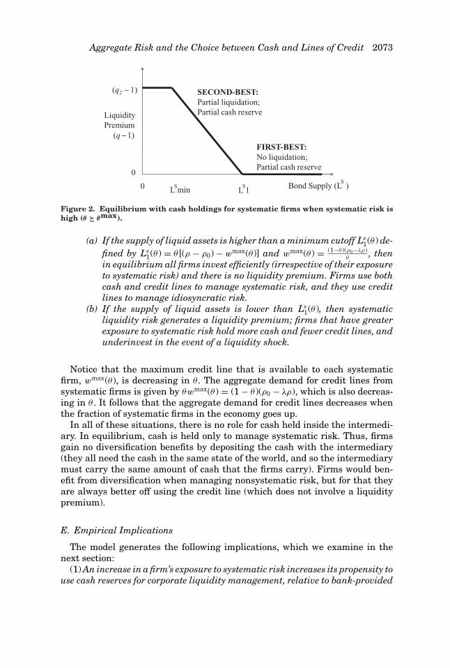
Figure 2. Equilibrium with cash holdings for systematic firms when systematic risk ishigh (θ ≥ θmax).

(a) If the supply of liquid assets is higher than a minimum cutoff Ls1(θ ) de-

fined by Ls1(θ ) = θ [(ρ − ρ0) − wmax(θ )] and wmax(θ ) = (1−θ)(ρ0−λρ)

θ, then

in equilibrium all firms invest efficiently (irrespective of their exposureto systematic risk) and there is no liquidity premium. Firms use bothcash and credit lines to manage systematic risk, and they use creditlines to manage idiosyncratic risk.

(b) If the supply of liquid assets is lower than Ls1(θ ), then systematic

liquidity risk generates a liquidity premium; firms that have greaterexposure to systematic risk hold more cash and fewer credit lines, andunderinvest in the event of a liquidity shock.

Notice that the maximum credit line that is available to each systematicfirm, wmax(θ ), is decreasing in θ . The aggregate demand for credit lines fromsystematic firms is given by θwmax(θ ) = (1 − θ )(ρ0 − λρ), which is also decreas-ing in θ . It follows that the aggregate demand for credit lines decreases whenthe fraction of systematic firms in the economy goes up.

In all of these situations, there is no role for cash held inside the intermedi-ary. In equilibrium, cash is held only to manage systematic risk. Thus, firmsgain no diversification benefits by depositing the cash with the intermediary(they all need the cash in the same state of the world, and so the intermediarymust carry the same amount of cash that the firms carry). Firms would ben-efit from diversification when managing nonsystematic risk, but for that theyare always better off using the credit line (which does not involve a liquiditypremium).

E. Empirical Implications

The model generates the following implications, which we examine in thenext section:

(1) An increase in a firm’s exposure to systematic risk increases its propensity touse cash reserves for corporate liquidity management, relative to bank-provided


lines of credit. We test this prediction by relating the fraction of total corporateliquidity held in the form of credit lines to proxies for a firm’s systematic riskexposure (e.g., beta).

(2) A firm’s exposure to risks that are systematic to the banking industryis particularly important for the determination of its liquidity policy. In themodel, bank systematic risk has a one-to-one relation with firm systematicrisk, given that there is only one source of risk in the economy (firms’ liquidityshock). However, one might imagine that in reality banks face other sources ofsystematic risk (coming, for example, from consumers’ liquidity demand) andthat firms are differentially exposed to such risks. Accordingly, a “firm-bankasset beta” should also drive corporate liquidity policy. Firms that are moresensitive to banking industry downturns should be more likely to hold cash forliquidity management.

(3) The trade-off between cash and credit lines is more important for firmsthat find it more costly to raise external capital. In the absence of financingconstraints, there is no role for corporate liquidity policy, and thus the choicebetween cash and credit lines becomes irrelevant. We test this model implica-tion by sorting firms according to observable proxies for financing constraints,and examining whether the effect of systematic risk exposure on the choicebetween cash and credit lines is driven by firms that are likely to be financiallyconstrained.

(4) The effect of systematic risk exposure on corporate liquidity policy shouldbe greater among firms with high systematic risk. In the model, the effect ofsystematic risk on corporate liquidity policy is nonlinear (convex). If aggregaterisk exposure is low (for example, if θ is low), then the bank’s liquidity constraintdoes not bind and hence variation in systematic risk exposure does not matter.After θ reaches the threshold level θmax, further increases in aggregate riskexposure tighten the bank’s liquidity constraint and thus force firms to switchto cash holdings. We test this implication by examining whether the effect ofaggregate risk exposure (beta) on liquidity policy is concentrated among firmswith high systematic risk exposure (e.g., beta).7

(5) Firms with higher systematic risk exposure should face worse contractualterms when raising bank credit lines. In the model, if the amount of systematicrisk in the economy is high, then the bank’s liquidity constraint requires thatcredit line contracts discriminate between idiosyncratic and systematic risk.Systematic firms should face worse contractual terms since they are the onesthat drive the bank’s liquidity constraint. We test this implication by relatingasset beta to credit line spreads and fees, after controlling for firm character-istics and other credit line contractual terms.

7 Strictly speaking, in the model the variable θ captures the amount of systematic risk in theeconomy as a whole. In addition, the model only allows for two types of firms (systematic andidiosyncratic). However, a similar implication would hold in a version of the model in which firmsvaried continuously with respect to their aggregate risk exposure. Low beta firms create littleliquidity risk for the bank, and thus there would be a cutoff below which all firms would haveaccess to cheap credit lines. Only high beta firms would be driven out of bank credit lines, andmore so the greater the value of beta.


(6) An increase in the amount of systematic risk in the economy increasesfirms’ reliance on cash and reduces their reliance on credit lines for liquiditymanagement. The model shows that, when economy-wide aggregate risk is low,firms can manage their liquidity using only credit lines because the bankingsector can provide such lines at actuarially fair terms. When aggregate riskincreases beyond a certain level, firms must shift away from credit lines andtoward cash so that the banking sector’s liquidity constraint is satisfied.8 Inaddition, the greater is the amount of systematic risk in the economy, thelower is the amount of liquidity that is provided by bank credit lines. We testthis implication by examining how aggregate cash holdings and credit lineinitiations change with VIX, the implied volatility of the stock market indexreturns from options data. In addition, and similarly to Implication 2 above,we examine whether Bank VIX, a measure of the expected volatility in thebanking sector, drives time-series variation in corporate liquidity policy.

(7) An increase in the amount of systematic risk in the economy worsens firms’contractual terms when raising bank credit lines. We test this implication byexamining how credit line spreads and maturities change with changes ineconomy-wide risk (VIX) and banking sector aggregate risk (Bank VIX).9

II. Empirical Tests

A. Data

We use two alternative sources to construct our line of credit data. Ourfirst sample (which we call LPC Sample) is drawn from LPC-DealScan. Thesedata allow us to construct a large sample of credit line initiations. We note,however, that the LPC-DealScan data have two potential drawbacks. First,they are mostly based on syndicated loans, and thus are potentially biasedtoward large deals and consequently toward large firms. Second, they do notallow us to measure line of credit drawdowns (the fraction of existing linesthat has been used in the past). To overcome these issues, we also constructan alternative sample that contains detailed information on the credit linesinitiated and used by a random sample of 300 COMPUSTAT firms. These dataare provided by Amir Sufi on his website and are used in Sufi (2009). We callthis sample Random Sample. Using these data reduces the sample size forour tests. In particular, since this sample only contains seven years (1996 to2003), in our time-series tests we use only LPC Sample. We regard these twosamples as providing complementary information on the use of credit lines for

8 In Section C.3, we provide evidence that exposure to undrawn corporate credit lines increasesbank stock return volatility in times of high aggregate risk. This result is consistent with themechanism suggested by the model, whereby credit line exposure poses risks to banks whencorporate liquidity shocks become correlated.

9 Our model has the additional empirical implication that the liquidity risk premium is higherwhen there is an economic downturn since in such times there is greater aggregate risk and linesof credit become more expensive. This is similar to the result of Eisfeldt and Rampini (2010), but intheir model the effect arises from the fact that firms’ cash flows are lower in economic downturnsand they are less naturally hedged against future liquidity needs.


the purposes of this paper. The data construction criteria are described in detailin Appendix B.

B. Variable Definitions

Our main variables of interest are described below. All of our control variablesin the tests are as in Sufi (2009). Detailed descriptions of the variables are inAppendices C, D, and E.

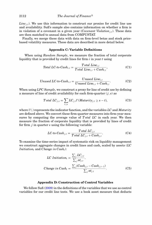
Line of credit data. When using Random Sample, we measure the fractionof total corporate liquidity provided by credit lines for firm i in year t usingthe ratios of both total and unused credit lines to the sum of credit lines pluscash. As discussed by Sufi, while some firms may have higher demand fortotal liquidity due to better investment opportunities, these LC-to-Cash ratiosshould isolate the relative use of lines of credit versus cash in corporate liquiditymanagement.

When using LPC Sample, we construct a proxy for line of credit usage in thefollowing way. For each firm-quarter, we measure credit line availability at datet by summing all existing credit lines that have not yet matured (Total LC).We convert these firm-quarter measures into firm-year measures by computingthe average value of Total LC in each year. We then measure the fraction ofcorporate liquidity provided by lines of credit by computing the ratio of TotalLC to the sum of Total LC plus cash.

In addition, to examine the time-series impact of systematic risk on liquiditymanagement we construct aggregate changes in credit lines and cash, scaled byassets (LC Initiationt and Change inCasht). These ratios capture the economy’stotal demand for cash and credit lines in a given year, scaled by total assets.

Data on betas and variances. We measure firms’ exposure to systematic riskusing asset (unlevered) betas.10 While equity betas are easy to compute usingstock price data, they are mechanically related to leverage: high leverage firmstend to have larger betas. Because greater reliance on credit lines typicallyincreases the firm’s leverage, the leverage effect would then bias our estimatesof the effect of betas on corporate liquidity management. Nonetheless, we alsopresent results using standard equity betas (Beta Equity).

We unlever equity betas in two alternative ways. First, we use a Merton-KMV-type model to unlever betas (Beta KMV) and total asset volatility (VarKMV). Second, we use Choi (2009) betas and asset variance (denoted BetaAsset and Var Asset). Because of data availability, we use Beta KMV as ourbenchmark measure of beta, but we verify that the results are robust to theuse of this alternative unlevering method.

One potential concern with these beta measures is that they may be me-chanically influenced by a firm’s cash holdings. Since corporate cash holdingsare typically held in the form of riskless securities, high cash firms could have

10 Similar to the COMPUSTAT data items, all measures of beta described below are winsorizedat the 5% level.


lower asset betas. Thus, we also compute KMV-type asset betas that are un-levered using net debt (e.g., debt minus cash) rather than gross debt. We callthis variable Beta Cash, which is computed at the industry level to mitigateendogeneity. We also compute a firm’s “bank beta” (which we call Beta Bank)to test the model’s implication that a firm’s exposure to the banking sector’srisks should influence the firm’s liquidity policy. In the model, a firm’s exposureto systematic risks matters mostly on the downside (because a firm may needliquidity when other firms are likely to be in trouble). To capture a firm’s expo-sure to large negative shocks, we follow Acharya et al. (2010) and compute thefirm’s Beta Tail.

All of the betas described above are computed using market prices. As dis-cussed in the introduction, market data are desirable because of their highfrequency, and because they also reflect a firm’s financing capacity that is tiedto its long-run prospects. However, the model’s argument is based on the cor-relation between a firm’s liquidity needs and the liquidity need for the overalleconomy (which affects the banking sector’s ability to provide liquidity). Whilemarket-based betas should capture this correlation, it is desirable to verifywhether a beta that is based more directly on cash flows and financing needsalso contains information about a firm’s choices between cash and credit lines.In order to do this, we compute two alternative beta proxies (Beta Gap andBeta Cash Flow).

Decomposing total risk into idiosyncratic and systematic components. In addi-tion to using asset and cash flow betas to measure systematic risk exposure,we alternatively use a measure of systematic risk that is computed by decom-posing total asset risk on its systematic and idiosyncratic components. Usingthe Merton-KMV betas and variances, the systematic component for firm j attime t can be estimated as

SysVar KMV j,t = (Beta KMV j,t

)2 × V ar KMVt, (19)

where V ar KMVt is the unlevered variance of the market. We computeV ar KMVt as the value-weighted average of firm-level asset variances,Var KMVj,t. The systematic component is essentially the variance of assetreturns that is explained by the market. Given this formula, the idiosyncraticcomponent can be computed as total asset variance V ar KMV j,t minus SysVarKMV j,t.

Notice that, since idiosyncratic variance is a function of total and systematicvariance, we do not need to include it separately in the corporate liquidityregressions. Rather, we experiment with specifications in which we include bothtotal and systematic variance (or beta) in the regressions explaining corporateliquidity.

Addressing measurement error. A common shortcoming of the measures of sys-tematic risk we construct is that they are noisy and subject to measurementerror. This problem can be ameliorated by adopting a strategy that deals withclassical errors-in-variables. We follow the standard Griliches and Hausman


(1986) approach to measurement problems and instrument the endogenousvariable (e.g., our beta proxies) with lags of itself. We experiment with alterna-tive lag structures and choose a parsimonious form that satisfies the restrictionconditions needed to validate the approach.11 Throughout the analysis, we re-port auxiliary statistics that speak to the relevance (first-stage F-tests) andvalidity (Hansen’s J-stats) of our instrumental variables regressions.

Time-series variables. We proxy for the extent of aggregate risk in the economyby using VIX (the implied volatility on S&P 500 index options). This variablecaptures both aggregate volatility as well as the financial sector’s appetiteto bear that risk. We also add other macroeconomic variables to our tests,including the commercial paper–Treasury spread (Gatev and Strahan (2006))to capture the possibility that funds may flow to the banking sector in timesof high aggregate volatility, and real GDP growth to capture general economicconditions.

In addition, we proxy for the extent of aggregate risk in the banking sectorby computing Bank VIX (the expected volatility on an index of bank stockreturns). Since there are no available historical data on implied volatility for anaggregate bank equity index, we compute expected volatility using a GARCH(1,1) model and the Fama-French index of bank stock returns. The InternetAppendix details the procedure that we use.

C. Empirical Tests and Results

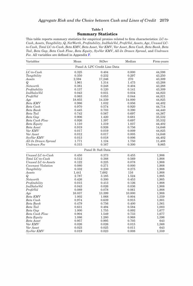
Summary statistics. We start by summarizing our data in Table I. Panel Areports summary statistics for the LPC-DealScan sample (for firm-years inwhich Beta KMV data are available), and Panel B uses Sufi’s sample. Noticethat the size of the sample in Panel A is much larger, and that the data forBeta Asset are available only for approximately one-third of the firm-years forwhich Beta KMV data are available. As expected, the average values of assetbetas are very close to each other, with average values close to one. The twoalternative measures of variance also appear to be very close to each other. Thespread and fee data are available at the deal level, and thus the number ofobservations reflects the number of different credit line deals in our sample.

Comparing Panel A and Panel B, notice that the distribution for most of thevariables is very similar across the two samples. The main difference betweenthe two samples is that the LPC-DealScan data are biased toward large firms(as discussed above). For example, median assets are equal to 270 millionin LPC Sample, and 116 million in Random Sample. Consistent with thisdifference, the firms in LPC Sample are also older, and have higher averageQs and EBITDA volatility. The measure of line of credit availability in LPCSample (LC-to-Cash) is lower than those in Random Sample (Total LC-to-Cashand Unused LC-to-Cash). For example, the average value of LC-to-Cash in

11 An alternative way to address measurement error is to compute betas at a “portfolio” level,rather than at the firm level. We explore this idea as well using industry betas rather than firm-level betas in some specifications below.


Table ISummary Statistics

This table reports summary statistics for empirical proxies related to firm characteristics: LC-to-Cash, Assets, Tangibility, Q, NetWorth, Profitability, IndSaleVol, ProfitVol, Assets, Age, Unused LC-to-Cash, Total LC-to-Cash, Beta KMV, Beta Asset, Var KMV, Var Asset, Beta Cash, Beta Bank, BetaTail, Beta Gap, Beta Cash Flow, Beta Equity, SysVar KMV, All-In Drawn Spread, and UndrawnFee. All variables are defined in Appendix F.

Variables Mean StDev Median Firm-years

Panel A: LPC Credit Line Data

LC-to-Cash 0.325 0.404 0.000 44,598Tangibility 0.350 0.232 0.297 43,250Assets 2,594 17,246 270 43,309Q 1.961 1.314 1.475 43,288Networth 0.381 0.248 0.404 43,288Profitability 0.137 0.120 0.141 43,309IndSalesVol 0.043 0.031 0.034 44,823ProfitVol 0.063 0.053 0.044 44,821Age 18.855 14.339 14.000 44,825Beta KMV 0.986 1.032 0.856 44,402Beta Cash 0.970 0.574 0.920 44,714Beta Bank 0.445 0.703 0.390 44,440Beta Tail 0.742 0.567 0.697 44,367Beta Gap 0.906 1.420 0.681 35,532Beta Cash Flow 0.926 1.397 0.697 35,532Beta Equity 1.110 1.319 1.037 44,402Beta Asset 0.919 0.926 0.756 14,646Var KMV 0.017 0.019 0.009 44,825Var Asset 0.012 0.017 0.005 14,646SysVar KMV 0.013 0.018 0.006 44,402All-In Drawn Spread 1.771 1.124 1.750 11,408Undrawn Fee 0.315 0.167 0.300 9,865

Panel B: Sufi Data

Unused LC-to-Cash 0.450 0.373 0.455 1,906Total LC-to-Cash 0.512 0.388 0.569 1,908Unused LC-to-Assets 0.122 0.225 0.078 1,908Covenant Violation 0.080 0.271 0.000 1,908Tangibility 0.332 0.230 0.275 1,908Assets 1,441 7,682 116 1,908Q 2.787 3.185 1.524 1,905Networth 0.426 0.300 0.453 1,905Profitability 0.015 0.413 0.126 1,908IndSalesVol 0.043 0.026 0.036 1,908ProfitVol 0.089 0.078 0.061 1,908Age 16.037 13.399 10.000 1,908Beta KMV 1.002 1.068 0.804 1,559Beta Cash 0.974 0.639 0.915 1,881Beta Bank 0.479 0.756 0.400 1,561Beta Tail 0.631 0.494 0.584 1,003Beta Gap 1.000 1.755 0.892 1,677Beta Cash Flow 0.904 1.549 0.733 1,677Beta Equity 1.086 1.280 0.968 1,596Beta Asset 0.957 0.995 0.705 643Var KMV 0.026 0.026 0.015 1,568Var Asset 0.023 0.025 0.011 643SysVar KMV 0.019 0.023 0.008 1,559


Table IICorrelations

This table shows the correlations for the different proxies for asset beta, idiosyncratic risk andsystematic risk. See Appendix F for a description of the variables.

Beta Beta Beta Beta Beta Beta Beta Beta Var SysVarAsset Cash Bank Tail Equity Gap Cash Flow KMV KMV KMV

Beta Cash 0.4627Beta Bank 0.5591 0.2795Beta Tail 0.4685 0.3302 0.2215Beta Equity 0.817 0.371 0.6213 0.3124Beta Gap 0.1809 0.232 0.0955 0.0863 0.0849Beta Cash Flow 0.1684 0.196 0.0982 0.0828 0.0747 0.6114Beta KMV 0.8889 0.4502 0.6416 0.3865 0.9444 0.1131 0.0925Var KMV 0.4001 0.2165 0.2585 0.2 0.2804 0.1144 0.096 0.3803SysVar KMV 0.7086 0.3469 0.463 0.2859 0.596 0.1285 0.0977 0.7374 0.6337Var Assets 0.4414 0.238 0.2633 0.2584 0.2978 0.1511 0.1491 0.3872 0.9181 0.6149

LPC Sample is 0.33, while the average value of Total LC-to-Cash is 0.51. Thisdifference reflects the fact that LPC-DealScan may fail to report some creditlines that are available in Sufi’s data, though it could also reflect the differentsample compositions.

In Table II, we examine the correlation among the different betas that we usein this study. We also include the asset variance proxies (Var KMV, Var Asset,and SysVar KMV). Not surprisingly, all the beta proxies that are based on assetreturn data are highly correlated. The lowest correlations are those betweenthe cash flow-based betas (Beta Gap and Beta Cash Flow) and the asset return-based betas (approximately 0.10). The correlations among the other betas (allbased on asset return data) range from 0.3 to 0.9.

To examine the effect of aggregate risk on the choice between cash and creditlines, we perform a number of different tests. We describe these tests in turn.

C.1. Firm-Level Regressions

Our benchmark empirical specification closely follows Sufi (2009). We expandhis specification by including our measure of systematic risk,

LC-to-Cashi,t =α + β1Beta KMVi,t + β2 ln(Age)i,t + β3( Profitability)i,t−1

+ β4Sizei,t−1 + β5 Qi,t−1 + β6 Networthi,t−1 + β7 IndSalesV olj,t

+ β8ProfitV oli,t +∑

t

Y eart + εi,t, (20)

where Year absorbs time-specific effects. Our theory predicts that the coefficientβ1 should be negative. We also run the same regression replacing Beta KMVwith our other proxies for a firm’s exposure to systematic and idiosyncraticrisks (see Section II.B). And we use different proxies for LC-to-Cash, whichare based on both LPC-DealScan and Sufi’s data. We further include industry


Table IIIThe Choice between Cash and Credit Lines: LPC-Deal Scan Sample

This table reports regressions of a measure of line of credit use in corporate liquidity policy onproxies for asset beta, asset variance, and controls. The dependent variable is LC-to-Cash, definedin Appendix F. Beta KMV is the firm’s asset (unlevered) beta, calculated from equity (levered)betas and a Merton-KMV formula. Var KMV is the corresponding value for total asset variance.SysVar KMV is a measure of firm-level systematic variance of asset returns. All proxies for Betaand variances are instrumented with their first two lags. All other variables are described inAppendix F. Robust t-statistics are presented in parentheses. *significant at 10%; **significant at5%; ***significant at 1%.

Dependent Variable: LC-to-Cash

(1) (2) (3) (4) (5)

Beta KMV −0.083*** −0.059*(−4.947) (−1.778)

Var KMV −3.920*** −1.681(−7.010) (−1.209)

SysVar KMV −6.213***(−8.231)

Profitability 0.136*** 0.031 0.101*** 0.044 0.063(5.435) (0.959) (3.274) (1.396) (1.633)

Tangibility 0.012 0.005 0.004 0.002 0.004(0.606) (0.215) (0.173) (0.072) (0.168)

Size 0.044*** 0.039*** 0.051*** 0.047*** 0.047***(16.151) (12.285) (16.151) (16.045) (8.726)

Networth −0.138*** −0.146*** −0.132*** −0.133*** −0.136***(−9.817) (−9.253) (−8.008) (−8.259) (−7.883)

Q −0.055*** −0.052*** −0.050*** −0.046*** −0.049***(−23.840) (−18.017) (−14.211) (−14.156) (−14.941)

IndSalesVol −0.197 −0.206 −0.219 −0.202 −0.208(−1.343) (−1.271) (−1.349) (−1.241) (−1.279)

ProfitVol −0.250*** 0.148* 0.033 0.221** 0.121(−3.751) (1.673) (0.380) (2.492) (1.316)

Age −0.047*** −0.054*** −0.052*** −0.056*** −0.053***(−7.933) (−7.165) (−6.819) (−7.394) (−7.049)

Constant 0.379*** 0.568*** 0.465*** 0.514*** 0.511***(5.710) (7.307) (6.044) (6.704) (6.064)

Industry fixed effect Yes Yes Yes Yes YesYear fixed effect Yes Yes Yes Yes YesFirst-stage F-stat p-value 0.000 0.000 0.000 0.000Hansen J-stat p-value 0.001 0.385 0.001 0.013

Observations 43,009 35,374 35,372 35,372 35,372R2 0.173 0.167 0.168 0.169 0.169

dummies (following Sufi, we use one-digit SIC industry dummies) and thevariance measures based on stock and asset returns (Var KMV and Var Asset).

The results for the KMV-Merton betas and variances, and the LPC-DealScandata, are presented in Table III. In column (1), we replicate Sufi’s (2009) results(see his table 3). Just like Sufi, we find that profitable, large, low Q, low networth, and low cash flow volatility firms are more likely to use bank credit


lines. The fact that we can replicate Sufi’s results is important, given that ourdependent variable is not as precisely measured as that in Sufi. In column(2), we introduce asset variance (Var KMV) in the model. We find that VarKMV is negatively correlated with the LC-to-Cash ratio, and it drives out thesignificance of Sufi’s profit volatility variable. This finding suggests that VarKMV is a better measure of total risk than the profit volatility variable usedby Sufi.

Next, we introduce our measures of systematic risk in the regressions. Thecoefficient on Beta KMV in column (3) suggests that systematic risk is nega-tively related to the LC-to-Cash ratio. The size of the coefficient implies that aone-standard-deviation increase in asset beta (approximately one) decreases afirm’s reliance on credit lines by approximately 0.08 (about 20% of the standarddeviation of the LC-to-Cash variable). In column (4) we use SysVar KMV in theregressions rather than Beta KMV. The results again suggest that systematicrisk exposure is negatively correlated with the LC-to-Cash ratio. Finally, incolumn (5) we report a specification that includes both Beta KMV and Var KMVtogether in the same regressions. The coefficient on Beta KMV drops to ap-proximately −0.06 and continues to be statistically significant (t-stat equal to−1.78). The coefficient on Var KMV remains negative but is not statisticallysignificant.

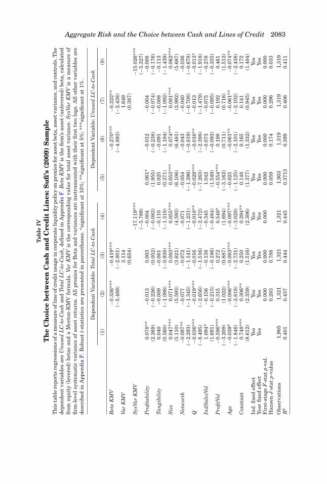
Table IV uses Sufi’s (2009) measures of LC-to-Cash rather than LPC-DealScan data. In columns (1) to (4) we use Total LC-to-Cash, and in columns(5) to (8) we use Unused LC-to-Cash. Columns (1) and (5) replicate the resultsin Sufi’s table 3. Notice that the coefficients are virtually identical to those inSufi. We next introduce our KMV-based proxies for total and aggregate riskexposures. As in Table III, the evidence suggests that systematic risk exposureis negatively correlated with the use of credit lines. We reach this conclusionboth when we use Beta KMV (columns (2) and (6)) and when we use SysVarKMV (columns (3) and (7)) to proxy for systematic risk exposure. In addition,aggregate risk exposure continues to be significantly related to the LC-to-Cashratio after controlling for Var KMV (columns (4) and (8)). These results suggestthat the cross-sectional relationship between systematic risk exposure and liq-uidity management is economically significant and robust to different ways ofcomputing exposure to systematic risk and reliance on credit lines.12

It is important that we consider the validity of our instrumental variablesapproach to the mismeasurement problem. The first statistic we consider in thisexamination is the first-stage exclusion F-tests for our set of instruments. Theirassociated p-values are all lower than 1% (confirming the explanatory powerof our instruments). We also examine the validity of the exclusion restrictionsassociated with our set of instruments. We do so using Hansen’s (1982) J-test

12 In our model, both cash and credit lines are used by the firm to hedge liquidity shocks. Thisraises the question of whether derivatives-based hedging affects our results. We believe this isunlikely for a couple of reasons. First, notice that the use of derivatives and other forms of hedgingshould be reflected in the betas that we observe. Second, while derivatives hedging is only feasiblein certain industries (such as those that are commodity-intensive), our results hold across andwithin industries for a broad set of industries.

Aggregate Risk and the Choice between Cash and Lines of Credit 2083T

able

IVT

he

Ch

oice

bet

wee

nC

ash

and

Cre

dit

Lin

es:S

ufi

’s(2

009)

Sam

ple

Th

ista

ble

repo

rts

regr

essi

ons

ofa

mea

sure

ofli

ne

ofcr

edit

usa

gein

corp

orat

eli

quid

ity

poli

cyon

prox

ies

for

asse

tbet

a,as

setv

aria

nce

,an

dco

ntr

ols.

Th

ede

pen

den

tva

riab

les

are

Un

use

dL

C-t

o-C

ash

and

Tota

lL

C-t

o-C

ash

,defi

ned

inA

ppen

dix

F.B

eta

KM

Vis

the

firm

’sas

set

(un

leve

red)

beta

,cal

cula

ted

from

equ

ity

(lev

ered

)be

tas

and

aM

erto

n-K

MV

form

ula

.Var

KM

Vis

the

corr

espo

ndi

ng

valu

efo

rto

tal

asse

tva

rian

ce.S

ysVa

rK

MV

isa

mea

sure

offi

rm-l

evel

syst

emat

icva

rian

ceof

asse

tre

turn

s.A

llpr

oxie

sfo

rB

eta

and

vari

ance

sar

ein

stru

men

ted

wit

hth

eir

firs

ttw

ola

gs.A

llot

her

vari

able

sar

ede

scri

bed

inA

ppen

dix

F.R

obu

stt-

stat

isti

csar

epr

esen

ted

inpa

ren

thes

es.*

sign

ifica

nt

at10

%;*

*sig

nifi

can

tat

5%;*

**si

gnifi

can

tat

1%.

Dep

ende

nt

Var

iabl

e:To

tal

LC

-to-

Cas

hD

epen

den

tV

aria

ble:

Un

use

dL

C-t

o-C

ash

(1)

(2)

(3)

(4)

(5)

(6)

(7)

(8)

Bet

aK

MV

−0.3

36**

*−0

.419

***

−0.2

70**

*−0

.322

**(−

5.48

9)(−

2.80

1)(−

4.89

3)(−

2.43

8)Va

rK

MV

3.11

41.

649

(0.6

54)

(0.3

87)

Sys

Var

KM

V−1

7.11

9***

−15.

026*

**(−

5.78

9)(−

5.32

7)P

rofi

tabi

lity

0.07

8**

−0.0

130.

003

−0.0

040.

061*

−0.0

12−0

.004

−0.0

08(2

.269

)(−

0.22

6)(0

.052

)(−

0.08

3)(1

.955

)(−

0.23

8)(−

0.07

4)(−

0.17

6)T

angi

bili

ty0.

040

−0.0

89−0

.081

−0.1

100.

025

−0.0

91−0

.088

−0.1

13(0

.560

)(−

1.09

8)(−

0.93

8)(−

1.31

8)(0

.371

)(−

1.18

4)(−

1.09

2)(−

1.43

9)S

ize

0.04

7***

0.07

1***

0.08

3***

0.05

5***

0.05

3***

0.07

4***

0.08

1***

0.06

2***

(5.1

10)

(5.5

93)

(3.6

21)

(4.5

93)

(6.1

06)

(6.4

81)

(3.9

92)

(5.6

87)

Net

wor

th−0

.097

**−0

.077

−0.0

72−0

.071

−0.0

54−0

.043

−0.0

40−0

.036

(−2.

293)

(−1.

345)

(−1.

141)

(−1.

231)

(−1.

396)

(−0.

819)

(−0.

708)

(−0.

678)

Q−0

.036

***

−0.0

19**

*−0

.016

−0.0

18**

−0.0

29**

*−0

.016

**−0

.013

−0.0

13*

(−8.

495)

(−2.

656)

(−1.

516)

(−2.

472)

(−7.

263)

(−2.

398)

(−1.

479)

(−1.

918)

Ind

Sal

esVo

l1.

094*

−0.1

56−0

.138

−0.3

451.

042

−0.0

73−0

.075

−0.2

78(1

.691

)(−

0.21

5)(−

0.18

6)(−

0.48

4)(1

.549

)(−

0.09

3)(−

0.09

5)(−

0.35

5)P

rofi

tVol

−0.5

96**

*0.

315

0.27

20.

548*

−0.5

54**

*0.

198

0.19

20.

461

(−3.

209)

(1.0

22)

(0.8

87)

(1.6

94)

(−3.

162)

(0.7

11)

(0.7

16)

(1.5

12)

Age

−0.0

39*

−0.0

86**

*−0

.083

***

−0.0

97**

*−0

.023

−0.0

61**

−0.0

61**

−0.0

74**

(−1.

846)

(−2.

818)

(−2.

731)

(−3.

028)

(−1.

125)

(−2.

101)

(−2.

102)

(−2.

438)

Con

stan

t0.

748*

**0.

306*

*0.

250

0.29

4**

0.14

80.

165

0.14

10.

172

(8.6

12)

(2.3

59)

(1.5

16)

(2.3

06)

(1.3

77)

(1.3

32)

(0.9

45)

(1.4

04)

Ind.

fixe

def

fect

Yes

Yes

Yes

Yes

Yes

Yes

Yes

Yes

Year

fixe

def

fect

Yes

Yes

Yes

Yes

Yes

Yes

Yes

Yes

Fir

st-s

tage

F-s

tat

p-va

l.0.

000

0.00

00.

000

0.00

00.

000

0.00

00.

000

Han

sen

J-s

tat

p-va

lue

0.28

30.

788

0.05

90.

174

0.29

60.

033

Obs

erva

tion

s1,

905

1,32

11,

321

1,32

11,

903

1,31

91,

319

1,31

9R

20.

401

0.43

70.

444

0.44

50.

3713

0.39

90.

406

0.41

1


statistic for overidentifying restrictions. The p-values associated with Hansen’stest statistic are reported in the last row of Tables III and IV. We generallyfind high p-values (particularly when using Sufi’s sample in Table V). Thesereported statistics suggest that we do not reject the joint null hypothesis thatour instruments are uncorrelated with the error term in the leverage regressionand the model is well-specified.

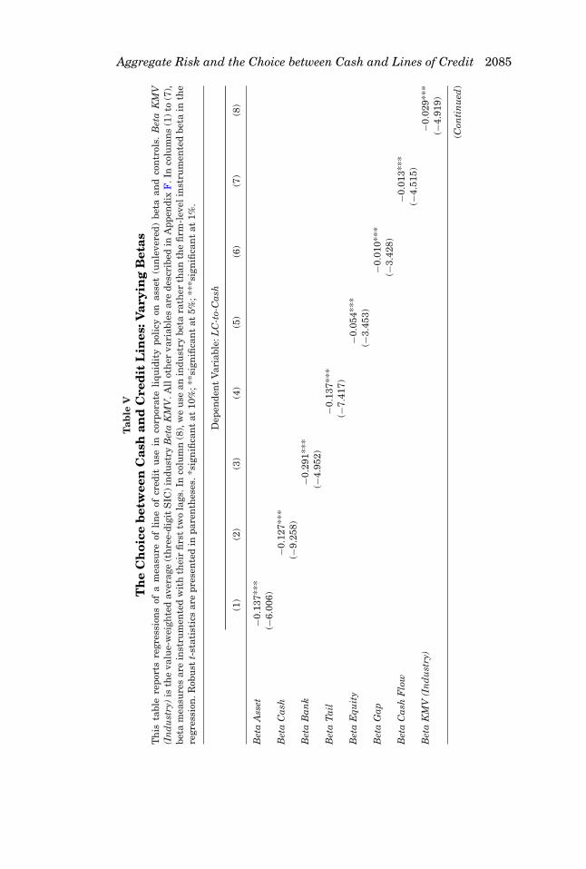
Table V replaces Beta KMV with our alternative beta measures using theLPC-Deal Scan sample.13 The results in the first column of Table V suggestthat the results reported in Table III are robust to the method used to unleverbetas. In particular, Beta Asset (which is based directly on asset return data) hasa similar relation to liquidity policy as that uncovered in Table II. The economicmagnitude of the coefficient on Beta Asset is in fact larger than that reportedin Table II. Using industry-level cash-adjusted betas, Beta Cash, also producessimilar results (column (2)). In column (3), we show that a firm’s exposureto banking sector risks (Beta Bank) affects liquidity policy in a way that isconsistent with the theory. The coefficients are also economically significant.Specifically, a one-standard-deviation increase in Beta Bank (which is equal to0.7) decreases LC-to-Cash by 0.21, which is half of the standard deviation ofthe LC-to-Cash variable. Column (4) shows that a firm’s exposure to tail risksis also correlated with liquidity policy. Firms that tend to do poorly duringmarket downturns have a significantly lower LC-to-Cash ratio. In column (5),we use equity (levered) betas instead of asset betas. The coefficient on beta iscomparable to the similar specification in Table III (which is in column (3)),though somewhat smaller. Thus, adjusting for the leverage effect increases theeffect of beta on the LC-to-Cash ratio (as expected). However, even the equitybeta shows a negative relation to the fraction of credit lines used in liquiditymanagement. Columns (6) and (7) replace market-based beta measures withcash flow-based betas computed at the industry level (Beta Gap and Beta CashFlow). Consistent with the theory, cash flow betas are significantly relatedto the LC-to-Cash ratio, though economic significance is smaller than for themarket measures.14 Finally, in column (8) we use value-weighted industrybetas rather than firm-level betas in the regression. Using industry betas is analternative way to address the possibility that firm-level betas are measuredwith error. Thus, in column (6) we do not instrument betas with the first twolags (as we do in the other columns). The results again suggest a significantrelation between asset beta and the LC-to-Cash ratio.

The regressions in Tables III and IV suggest that total risk is not robustlyrelated to corporate liquidity policy, after introducing proxies for systematicrisk exposure (such as Beta KMV). In other words, firms’ idiosyncratic or non-systematic risk is not robustly related to cross-sectional variation in liquiditypolicy. This result may appear to contradict the results in Sufi (2009), whosuggests that riskier firms should shy away from credit lines due to the risk

13 We obtain similar results when using Sufi’s sample (see the Internet Appendix).14 The coefficient in column (7), for example, suggests that a one-standard-deviation increase in

Beta Gap decreases LC-to-Cash by approximately 1.5%.


Tab

leV

Th

eC

hoi

ceb

etw

een

Cas

han

dC

red

itL

ines

:Var

yin

gB

etas

Th

ista

ble

repo

rts

regr

essi

ons

ofa

mea

sure

ofli

ne

ofcr

edit

use

inco

rpor

ate

liqu

idit

ypo

licy

onas

set

(un

leve

red)

beta

and

con

trol

s.B

eta

KM

V(I

nd

ust

ry)

isth

eva

lue-

wei

ghte

dav

erag

e(t

hre

e-di

git

SIC

)in

dust

ryB

eta

KM

V.A

llot

her

vari

able

sar

ede

scri

bed

inA

ppen

dix

F.I

nco

lum

ns

(1)

to(7

),be

tam

easu

res

are

inst

rum

ente

dw

ith

thei

rfi

rst

two

lags

.In

colu

mn

(8),

we

use

anin

dust

rybe

tara

ther

than

the

firm

-lev

elin

stru

men

ted

beta

inth

ere

gres

sion

.Rob

ust

t-st

atis

tics

are

pres

ente

din

pare

nth

eses

.*si

gnifi

can

tat

10%

;**s

ign

ifica

nt

at5%

;***

sign

ifica

nt

at1%

.

Dep

ende

nt

Var

iabl

e:L

C-t

o-C

ash

(1)

(2)

(3)

(4)

(5)

(6)

(7)

(8)

Bet

aA

sset

−0.1

37**

*(−

6.00

6)B

eta

Cas

h−0

.127

***

(−9.

258)

Bet

aB

ank

−0.2

91**

*(−

4.95

2)B

eta

Tai

l−0

.137

***

(−7.

417)

Bet

aE

quit

y−0

.054

***

(−3.

453)

Bet

aG

ap−0

.010

***

(−3.

428)

Bet

aC

ash

Flo

w−0

.013

***

(−4.

515)

Bet

aK

MV

(In

du

stry

)−0

.029

***

(−4.

919)

(Con

tin

ued

)


Tab

leV

I—C

onti

nu

ed

Dep

ende

nt

Var

iabl

e:L

C-t

o-C

ash

(1)

(2)

(3)

(4)

(5)

(6)

(7)

(8)

Pro

fita

bili

ty0.

042

0.11

6***

0.07

8**

0.12

8***

0.11

3***

0.11

7***

0.11

8***

0.12

4***

(0.6

75)

(5.0

88)

(2.2

84)

(4.3

64)

(3.8

78)

(4.7

79)

(4.8

53)

(5.0

08)

Tan

gibi

lity

−0.0

17−0

.004

−0.0

15−0

.001

0.00

60.

025

0.02

60.

048*

*(−

0.40

0)(−

0.23

9)(−

0.62

9)(−

0.02

7)(0

.269

)(1

.320

)(1

.372

)(2

.400

)S

ize

0.04

2***

0.05

0***

0.05

5***

0.05

9***

0.05

2***

0.04

9***

0.04

9***

0.04

2***

(6.9

65)

(19.

963)

(15.

334)

(16.

679)

(15.

804)

(17.

865)

(17.

905)

(14.

520)

Net

wor

th−0

.127

***

−0.1

09**

*−0

.120

***

−0.1

18**

*−0

.149

***

−0.1

24**

*−0

.125

***

−0.1

14**

*(−

4.16

9)(−

8.61

2)(−

6.83

6)(−

7.16

9)(−

9.72

0)(−

9.08

0)(−

9.16

2)(−

8.20

4)Q

−0.0

50**

*−0

.049

***

−0.0

48**

*−0

.044

***

−0.0

53**

*−0

.056

***

−0.0

56**

*−0

.052

***

(−8.

136)

(−23

.028

)(−

12.1

98)

(−12

.330

)(−

17.6

81)

(−25

.415

)(−

25.5

07)

(−22

.093

)In

dS

ales

Vol

−0.3

41−0

.128

−0.1

56−0

.174

−0.1

90−0

.187

−0.1

720.

132

(−1.

029)

(−1.

066)

(−0.

936)

(−1.

063)

(−1.

207)

(−1.

356)

(−1.

255)

(0.8

26)

Pro

fitV

ol−0

.315

*−0

.013

0.12

00.

065

−0.0

65−0

.254

***

−0.2

54**

*−0

.198

***

(−1.

747)

(−0.

199)

(1.1

68)

(0.7

97)

(−0.

780)

(−3.

608)

(−3.

592)

(−2.

785)

Age

−0.0

29**

−0.0

48**

*−0

.054

***

−0.0

53**

*−0

.053

***

−0.0

42**

*−0

.043

***

−0.0

46**

*(−

2.06

4)(−

8.49

4)(−

6.91

6)(−

7.00

5)(−

7.53

5)(−

6.67

8)(−

6.71

0)(−

6.90

2)C

onst

ant

0.44

8**

0.61

4***

0.46

8***

0.41

5***

0.47

7***

0.45

3***

0.45

4***

0.36

2***

(2.5

29)

(21.

435)

(5.8

00)

(5.6

13)

(6.4

72)

(16.

661)

(16.

738)

(13.

516)

Indu

stry

fixe

def

fect

Yes

No

Yes

Yes

Yes

No

Yes

No

Year

fixe

def

fect

Yes

Yes

Yes

Yes

Yes

Yes

Yes

Yes

Fir

st-s

tage

F-s

tat

p-va

lue

0.00

00.

000

0.00

00.

000

0.00

00.

000

0.00

0H

anse

nJ

-sta

tp-

valu

e0.

158

0.00

50.

586

0.00

00.

156

0.87

280.

001

Obs

erva

tion

s9,

536

46,8

6535

,499

35,3

4338

,397

37,4

8537

,485

31,8

1131

,811

R2

0.21

10.

162

0.16

60.

170

0.16

60.

155

0.15

50.

166


of covenant violations. However, Sufi (2009) also shows that the level of prof-itability proxies for the risk of covenant violations and credit line revocations.In particular, the level of profitability is the key variable that predicts covenantviolations (as shown in Sufi’s table 6). The results above are consistent withSufi’s profitability results, since the level of profitability in our results is alsopositively related to the LC-Cash ratio, particularly so in the LPC Sample(Tables III and V), suggesting that the risk of credit line revocation is beingcaptured by variation in the level of profitability, rather than nonsystematicrisk.

Sorting firms according to proxies for financing constraints and beta. One ofthe implications of the model in Section I is that the choice between cash andcredit lines should be most relevant for firms that are financially constrained(Implication 3). This line of argument suggests that the relation we find aboveshould be driven by firms that find it more costly to raise external funds. Inaddition, the theory suggests that the effect of systematic risk exposure on cor-porate liquidity policy should primarily arise among firms with high systematicrisk (Implication 4). In this section we attempt to test both implications. Wefollow prior studies (e.g., Almeida, Campello, and Weisbach (2004)) in usingthree alternative schemes to partition our sample in order to test Implication3: (1) We rank firms based on their payout ratio and assign to the financiallyconstrained (unconstrained) group those firms in the bottom (top) three decilesof the annual payout distribution.

(2) We rank firms based on their asset size, and assign to the financiallyconstrained (unconstrained) group those firms in the bottom (top) three decilesof the size distribution. The argument for size as a good observable measureof financial constraints is that small firms are typically young and less wellknown, and thus more vulnerable to credit imperfections.

(3) We rank firms based on whether they have bond and commercial paperratings. A firm is deemed to be constrained if it has neither a bond nor a com-mercial paper rating; it is unconstrained if it has both a bond and a commercialpaper rating.

To test Implication 4, we partition the sample into two groups. “high beta”firms are those that have beta greater than one. “low beta” firms are thosethat have beta less than one (the average value of Beta KMV according toTable I).

We repeat the regressions performed above, but now separately for finan-cially constrained and unconstrained subsamples and for low beta and highbeta subsamples. To measure systematic risk, we use both Beta KMV and BetaTail (which measures firms’ exposure to tail risks).

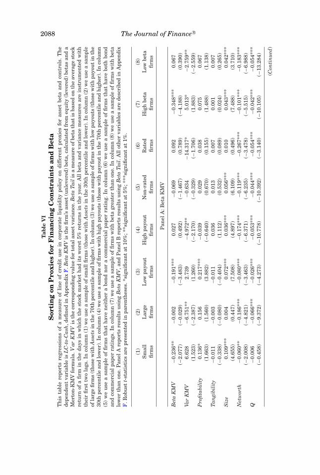
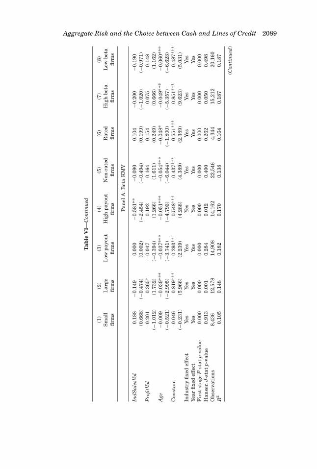
Table VI presents the results we obtain. Panel A presents results for BetaKMV, and Panel B shows the Beta Tail results. Results for the other beta prox-ies are generally similar, and are presented in the Internet Appendix. The firstsix columns in Panel A show that the negative relation between systematic riskand the use of credit lines obtains only in the constrained samples. The coeffi-cient on Beta KMV for the constrained samples is negative and significant forthe small and low payout samples, but is insignificant for large, high payout,


Tab

leV

IS

orti

ng

onP

roxi

esfo

rF

inan

cin

gC

onst

rain

tsan

dB

eta

Th

ista

ble

repo

rts

regr

essi

ons

ofa

mea

sure

ofli

ne

ofcr

edit

use

inco

rpor

ate

liqu

idit

ypo

licy

ondi

ffer

ent

prox

ies

for

asse

tbe

taan

dco

ntr

ols.

Th

ede

pen

den

tva

riab

leis

LC

-to-

Cas

h,d

efin

edin

App

endi

xF

.Bet

aK

MV

isth

efi

rm’s

asse

t(u

nle

vere

d)be

ta,c

alcu

late

dfr

omeq

uit

y(l

ever

ed)b

etas

and

aM

erto

n-K

MV

form

ula

.Var

KM

Vis

the

corr

espo

ndi

ng

valu

efo

rto

tala

sset

vari

ance

.Bet

aT

aili

sa

mea

sure

ofbe

tath

atis

base

don

the

aver

age

stoc

kre

turn

ofa

firm

inth

eda

ysin

wh

ich

the

stoc

km

arke

th

adit

sw

orst

5%re

turn

sin

the

year

.All

beta

and

vari

ance

mea

sure

sar

ein

stru

men

ted

wit

hth

eir

firs

ttw

ola

gs.I

nco

lum

n(1

)w

eu

sea

sam

ple

ofsm

allfi

rms

(th

ose

wit

hA

sset

sin

the

30th

perc

enti

lean

dlo

wer

).In

colu

mn

(2)

we

use

asa

mpl

eof

larg

efi

rms

(th

ose

wit

hA

sset

sin

the

70th

perc

enti

lean

dh

igh

er).

Inco

lum

n(3

)we

use

asa

mpl

eof

firm

sw

ith

low

payo

uts

(th

ose

wit

hpa

you

tin

the

30th

perc

enti

lean

dlo

wer

).In

colu

mn

(4)w

eu

sea

sam

ple

offi

rms

wit

hh

igh

payo

uts

(th

ose

wit

hpa

you

tin

the

70th

perc

enti

lean

dh

igh

er).

Inco

lum

n(5

)w

eu

sea

sam

ple

offi

rms

that

hav

en

eith

era

bon

dn

ora

com

mer

cial

pape

rra

tin

g.In

colu

mn

(6)

we

use

asa

mpl

eof

firm

sth

ath

ave

both

bon

dan

dco

mm

erci

alpa

per

rati

ngs

.In

colu

mn

(7)

we

use

asa

mpl

eof

firm

sw

ith

beta

grea

ter

than

one.

Inco

lum

n(8

)w

eu

sea

sam

ple

offi

rms

wit

hbe

talo

wer

than

one.

Pan

elA

repo

rts

resu

lts

usi

ng

Bet

aK

MV

,an

dP

anel

Bre

port

sre

sult

su

sin

gB

eta

Tai

l.A

llot

her

vari

able

sar

ede

scri

bed

inA

ppen

dix

F.R

obu

stt-

stat

isti

csar

epr

esen

ted

inpa

ren

thes

es.*

sign

ifica

nt

at10

%;*

*sig

nifi

can

tat

5%;*

**si

gnifi

can

tat

1%.

(1)

(2)

(3)

(4)

(5)

(6)

(7)

(8)

Sm

all

Lar

geL

owpa

you

tH

igh

payo

ut

Non

-rat

edR

ated

Hig

hbe

taL

owbe

tafi

rms

firm

sfi

rms

firm

sfi

rms

firm

sfi

rms

firm

s

Pan

elA

:Bet

aK

MV

Bet

aK

MV

−0.2

36**

−0.0

02−0

.191

***

0.02

7−0

.069

0.09

2−0

.348

***

0.06

7(−

2.07

7)(−

0.02

9)(−

3.48

3)(0

.492

)(−

1.46

7)(0

.789

)(−

4.18

8)(0

.390

)Va

rK

MV

6.62

8−6

.751

**2.

739

−4.9

72**

−0.6

34−1

4.31

7*5.

013*

−2.7

59**

(1.5

23)

(−2.

387)

(1.2

60)

(−2.

170)

(−0.

329)

(−1.

706)

(1.8

83)

(−2.

559)

Pro

fita

bili

ty0.

136*

0.15

60.

217*

**−0

.039

0.02

90.

038

0.07

50.

067

(1.6

63)

(1.5

60)

(3.8

82)

(−0.

640)

(0.6

70)

(0.1

55)

(1.4

88)

(1.1

38)

Tan

gibi

lity

−0.0

11−0

.003

−0.0

110.

036

0.01

30.

007

0.00

10.

007

(−0.

338)

(−0.

080)

(−0.

404)

(1.1

12)

(0.5

32)

(0.0

89)

(0.0

24)

(0.2

65)

Siz

e0.

109*

**0.

004

0.07

2***

0.03

6***

0.05

6***

0.01

00.

043*

**0.

042*

**(4

.655

)(0

.447

)(7

.508

)(4

.897

)(6

.109

)(0

.496

)(7

.488

)(3

.710

)N

etw

orth

−0.0

60**

−0.1

86**

*−0

.080

***

−0.1

74**

*−0

.119

***

−0.2

67**

*−0

.101

***

−0.1

83**

*(−

2.00

8)(−

4.82

1)(−

3.46

3)(−

6.37

1)(−

6.23

5)(−

3.47

8)(−

5.51

5)( −

6.98

8)Q

−0.0

06−0

.066

***

−0.0

26**

*−0

.053

***

−0.0

44**

*−0

.054

***

−0.0

42**

*−0

.054

***

(−0.

458)

(−9.

372)

(−4.

273)

(−10

.778

)(−

10.3

92)

(−3.

140)

(−10

.105

)(−

13.2

84)

(Con

tin

ued

)


Tab

leV

I—C

onti

nu

ed

(1)

(2)

(3)

(4)

(5)

(6)

(7)

(8)

Sm

all

Lar

geL

owpa

you

tH

igh

payo

ut

Non

-rat

edR

ated

Hig

hbe

taL

owbe

tafi

rms

firm

sfi

rms

firm

sfi

rms

firm

sfi

rms

firm

s

Pan

elA

:Bet

aK

MV

Ind

Sal

esVo

l0.

188

−0.1

490.

000

−0.5

81**

−0.0

900.

104

−0.2

00−0

.190

(0.6

68)

(−0.

474)

(0.0

02)

(−2.

454)

(−0.

494)

(0.1

99)

(−1.

020)

(−0.

971)

Pro

fitV

ol−0

.201

0.36

5*−0

.047

0.19

20.

164

0.15

40.

075

0.14

8(−

1.01

2)(1

.732

)(−

0.39

4)(1

.266

)(1

.611

)(0

.249

)(0

.666

)(1

.162

)A

ge−0

.009

−0.0

39**

*−0

.037

***

−0.0

51**

*−0

.054

***

−0.0

48*

−0.0

49**

*−0

.060

***

(−0.

521)

(−2.

995)

(−3.

741)

(−4.

793)

(−6.

044)

(−1.

800)

(−5.

357)

(−6.

623)

Con

stan

t−0

.046

0.81

9***

0.29

3**

0.54

8***

0.43

7***

0.55

1***

0.85

1***

0.48

7***

(−0.

231)

(5.9

66)

(2.2

39)

(4.2

88)

(4.3

89)

(2.3

89)

(9.6

23)

(5.0

31)

Indu

stry

fixe

def

fect

Yes

Yes

Yes

Yes

Yes

Yes

Yes

Yes

Year

fixe

def

fect

Yes

Yes

Yes

Yes

Yes

Yes

Yes

Yes

Fir

st-s

tage

F-s

tat

p-va

lue

0.00

00.

000

0.00

00.

000

0.00

00.

000

0.00

00.

000

Han

sen

J-s

tat

p-va

lue

0.91

30.

001

0.28

40.

012

0.40

00.

262

0.05

00.

498

Obs

erva

tion

s8,

436

12,5

7814

,908

14,1

6222

,546

4,34

415

,212

20,1

60R

20.

105

0.14

80.

182

0.17

00.

138

0.16

40.

187

0.18

7

(Con

tin

ued

)


Tab

leV

I—C

onti

nu

ed

(1)

(2)

(3)

(4)

(5)

(6)

(7)

(8)

Sm

all

Lar

geL

owpa

you

tH

igh

payo

ut

Non

-rat

edR

ated

Hig

hbe

taL

owbe

tafi

rms

firm

sfi

rms

firm

sfi

rms

firm

sfi

rms

firm

s

Pan

elB

:Bet

aTa

il

Bet

aT

ail

−0.2

28**

*−0

.019

−0.1

78**

*−0

.091

**−0

.151

***

0.07

7−0

.574

***

−0.1

62**

(−4.

518)

(−0.

385)

(−4.

452)

(−2.

481)

(−4.

556)

(0.7

36)

(−4.

793)

(−2.

525)

Var

KM

V2.

578*

−6.3

01**

*−0

.305

−1.7

870.

199

−12.

204*

1.14

5−1

.265

(1.8

33)

(−3.

194)

(−0.

260)

(−1.

319)

(0.1

93)

(−1.

766)

(0.6

54)

(−1.

260)

Pro

fita

bili

ty0.

133*

**0.

161

0.20

7***

0.01

30.

077*

0.06

10.

043

0.16

4***

(2.6

21)

(1.5

89)

(4.4

48)

(0.2

28)

(1.9

43)

(0.2

48)

(0.9

19)

(3.2

55)

Tan

gibi

lity

−0.0

10−0

.005

−0.0

120.

030

0.00

50.

008

−0.0

03−0

.010

(−0.

353)

(−0.

122)

(−0.

461)

(0.9

28)

(0.2

21)

(0.0

98)

(−0.

101)

(−0.

379)

Siz

e0.

109*

**0.

006

0.07

0***

0.04

8***

0.06

9***

0.00

60.

035*

**0.

064*

**(8

.191

)(0

.541

)(9

.223

)(7

.639

)(9

.636

)(0

.301

)(5

.622

)(8

.554

)N

etw

orth

−0.0

76**

*−0

.182

***

−0.0

83**

*−0

.150

***

−0.1

03**

*−0

.276

***

−0.0

64**

*−0

.143

***

(−3.

878)

( −4.

730)

(−4.

063)

(−5.

829)

(−5.

789)

(−3.

430)

(−3.

042)

(−6.

633)

Q−0

.003

−0.0

66**

*−0

.025

***

−0.0

48**

*−0

.036

***

−0.0

61**

*−0

.038

***

−0.0

51**

*(−

0.52

0)(−

9.07

2)(−

4.63

8)(−

9.65

0)(−

8.92

2)(−

4.13

6)(−

8.97

3)(−

12.1

36)

Ind

Sal

esVo

l0.

155

−0.1

420.

156

−0.5

60**

−0.0

730.

052

0.05

6−0

.296

(0.5

92)

(−0.

450)

(0.7

24)

(−2.

370)

(−0.

406)

(0.1

00)

(0.2

47)

(−1.

599)

Pro

fitV

ol0.

012

0.37

5*0.

079

0.16

10.

186*

*0.

179

0.19

50.

146

(0.0

95)

(1.7

93)

(0.7

73)

(1.0

62)

(1.9

72)

(0.2

91)

(1.6

06)

(1.2

97)

Age

−0.0

23*

−0.0

38**

*−0

.043

***

−0.0

50**

*−0

.057

***

−0.0

50*

−0.0

47**

*−0

.058

***

(−1.

679)

(−2.

956)

(−4.

465)

(−4.

736)

(−6.

458)

(−1.

852)

(−4.

391)

(−6.

768)

Con

stan

t0.

047

0.81

0***

0.33

4***

0.47

4***

0.35

8***

0.60

0***

1.20

3***

0.39

9***

(0.4

04)

(5.7

87)

(2.8

20)

(3.6

93)

(3.9

21)

(2.3

69)

(10.

152)

(4.2

53)

Indu

stry

fixe

def

fect

Yes

Yes

Yes

Yes

Yes

Yes

Yes

Yes

Year

fixe

def

fect

Yes

Yes

Yes

Yes

Yes

Yes

Yes

Yes

Fir

st-s

tage

F-s

tat

p-va

lue

0.00

00.

000

0.00

00.

000

0.00

00.

000

0.00

00.

000

Han

sen

J-s

tat

p-va

lue

0.08

40.

001

0.00

00.

076

0.00

00.

345

0.00

00.

0223

Obs

erva

tion

s8,

418

12,5

7314

,892

14,1

5122

,528

4,34

410

,679

24,6

64R

20.

108

0.14

90.

184

0.17

10.

140

0.16

40.

191

0.16

0


and rated firms. Column (5) shows that the coefficient is negative but not sig-nificant for nonrated firms (t-stat of 1.47). The coefficients are also significantlydifferent across constrained and unconstrained samples, with the exception ofthe ratings sorting. The p-values from Wald tests that the coefficients are sig-nificantly different from each other range from 0.198 (ratings sorting) to 0.005(payout sorting). Panel B shows similar results for the Beta Tail variable. Themain differences are that the coefficient on Beta Tail for the nonrated sub-sample is now significantly negative (t-stat of −4.56), while the coefficient forthe high-payout sample is now negative and significant. However, even for thepayout sorting there is (weak) evidence that the coefficient is larger for theconstrained sample. The p-value from a Wald test that the coefficient forthe low payout sample is different from that for the high payout sample is0.104. The p-values are higher for the ratings (p-value of 0.037) and the sizesortings (p-value of 0.003), indicating that the coefficient on beta for constrainedsamples is indeed more negative than that for unconstrained samples. Theseresults are consistent with Implication 3.

Columns (7) and (8) of each panel show that the negative relationship be-tween beta and the LC-Cash ratio is much stronger in the sample of firms withhigh exposure to aggregate risk. When using Beta KMV, the negative coeffi-cient on beta obtains only in the high beta sample. The coefficient is negativeand significant for the low beta sample when using Beta Tail, but its magni-tude is substantially smaller than the coefficient that obtains in the high betasample. The p-value from a Wald test that the coefficients on Beta Tail are dif-ferent from each other is 0.024, indicating that the coefficients are statiscallydistinguishable from each other. These results support Implication 4.

The nonlinearity of the relationship between beta and the LC-to-Cash ratiocan also be illustrated with a graph. In Figure 3, we sort the sample intoquintiles based on the average value for Beta KMV for each firm during theentire sample period. We then calculate the average value of the LC-to-Cashratio in each of these quintiles of beta. Figure 3 shows that the average LC-to-Cash ratio barely changes as one moves from the first to the third quintile ofbeta (the average LC-to-Cash ratio in the first three quintiles is approximately0.35). However, the average ratio in the highest quintile drops to less than0.2. This figure gives a visual illustration that the effect of beta on the LC-to-Cash ratio is concentrated among firms with high exposure to systematic risk(Implication 4 of the theory).

Asset beta and the cost of credit lines. The empirical findings so far all suggestthat firms with high aggregate risk exposure hold more cash relative to linesof credit. This effect arises in our theoretical model since firms with greateraggregate risk exposure face a higher cost of bank lines of credit. We performan additional test to further investigate this channel. Specifically, we provideevidence on the relation between all-in drawn spreads and undrawn fees paidby firms on their credit lines and systematic risk. To do so, we regress theaverage annual spreads and fees paid by firm i in deals initiated in year t15

15 This annual average is weighted by the amount raised in each credit line deal.


0

0.2

0.4

0.6

0.8

1

1.2

1.4

1.6

1.8

2

0

0.05

0.1

0.15

0.2

0.25

0.3

0.35

0.4

1 2 3 4 5

Beta

LC-Cash

Quin les of Beta

Figure 3. Average LC-Cash ratios for different quintiles of Beta KMV. This figure reportsthe average LC-Cash ratio for firms in different quintiles of Beta KMV. The sample is sorted intoquintiles based on the average value of Beta KMV for each firm during the entire sample period.We then calculate the average value of the LC-Cash ratio in each of these quintiles of beta.

on systematic risk proxies and controls. We control for the size of credit linefacilities raised in year t scaled by assets ( LCi,t

Assetsi,t), and the level of the LIBOR

in the quarter when the credit line was raised.16 Our empirical model has thefollowing form:

Costi,t = μ0 + μ1Betai,t + μ2

(LCi,t

Assetsi,t

)+ μ3LIBORi,t + μ4Xi,t

+∑

t

Y eart + εi,t, (21)

where X is the vector of firm characteristics used in equation (20). We use bothAll-in drawn spread and Undrawn fee as alternative dependent variables tomeasure the cost of credit lines. We focus on a set of three risk proxies (namely,Beta KMV, Beta Tail, and SysVar KMV), and present results for the otherproxies in the Internet Appendix.

Our findings are presented in Table VII. The coefficients on the systematicrisk proxies in columns (1) to (3) suggest that All-In-Drawn Spread is higher

16 The data on LIBOR refer to the level of LIBOR in the quarter in which firm i initiates thecredit line. We annualize this variable by computing the facility size-weighted, firm-year average(LIBORi,t). Notice that, since firms initiate credit lines in different quarters, this proxy varies bothover time and across firms.


Table VIIAggregate Risk Exposure and the Cost of Credit Lines

This table reports regressions of line of credit spreads and fees on systematic risk exposure andcontrols. LIBOR is the level of the LIBOR (in percentage) in the quarter in which a deal wasinitiated, for each firm. New LC is the total size of deals initiated in a firm-year, scaled by assets.All other variables are described in Appendix F. All proxies for beta are instrumented with theirfirst two lags. Robust z-statistics are presented in parentheses. *significant at 10%; **significantat 5%; ***significant at 1%.

Dependent Variables

All-In Drawn Spread Undrawn Fee

(1) (2) (3) (4) (5) (6)

Beta KMV 0.104 0.051***(1.525) (3.560)

SysVar KMV 10.029*** 3.124***(2.740) (4.047)

Beta Tail 0.142** 0.047***(2.347) (4.077)

LIBOR −0.005 −0.005 −0.001 0.003 0.001 0.005(−0.242) (−0.230) (−0.051) (0.631) (0.188) (1.291)

New LC −0.236*** −0.237*** −0.240*** −0.018*** −0.020*** −0.020***(−3.355) (−3.555) (−3.503) (−5.102) (−6.620) (−6.954)

Profitability −1.852*** −1.732*** −1.897*** −0.095*** −0.073** −0.120***(−11.885) (−10.871) (−12.435) (−3.163) (−2.359) (−4.351)

Tangibility 0.131** 0.142** 0.140** 0.027** 0.030** 0.030**(2.192) (2.390) (2.367) (2.205) (2.451) (2.555)

Size −0.368*** −0.362*** −0.376*** −0.046*** −0.044*** −0.049***(−45.526) (−48.126) (−41.431) (−27.482) (−26.389) (−26.738)

Networth −1.212*** −1.217*** −1.237*** −0.193*** −0.188*** −0.196***(−20.204) (−21.222) (−20.412) (−17.657) (−18.006) (−18.657)

Q −0.150*** −0.164*** −0.154*** −0.036*** −0.038*** −0.035***(−10.034) (−10.493) (−11.052) (−12.703) (−12.967) (−14.002)

IndSalesVol 0.238 0.219 0.131 −0.057 −0.046 −0.099(0.521) (0.488) (0.291) (−0.629) (−0.512) (−1.149)

ProfitVol 2.266*** 1.823*** 2.275*** 0.128* 0.047 0.173***(6.337) (4.695) (7.392) (1.880) (0.623) (2.978)

Constant 4.790*** 4.726*** 4.828*** 0.668*** 0.659*** 0.683***(21.626) (22.075) (22.695) (18.972) (19.000) (21.034)

Year fixed effect Yes Yes Yes Yes Yes YesIndustry fixed effect Yes Yes Yes Yes Yes YesFst.-stage F-stat p-val 0.000 0.000 0.000 0.000 0.000 0.000Hansen F-stat p-value 0.017 0.082 0.652 0.942 0.753 0.381

Observations 6,799 6,895 6,774 5,977 6,084 5,973R2 0.559 0.550 0.559 0.404 0.405 0.405

for firms with greater exposure to systematic risk (though statistical signifi-cance for the coefficient on Beta KMV is weaker).17 For example, the coefficientestimate of 10 on SysVar KMV indicates that a one-standard-deviation changein systematic risk exposure (equal to 0.018 according to Table I) is associatedwith an increase of 18 basis points on credit line spreads (approximately 16%of the standard deviation in All-In-Drawn Spread). Columns (4) through (6)show similar results for Undrawn Fee. The evidence suggests that an increase

17 We obtain generally similar results for the other systematic risk proxies (see the InternetAppendix).


of one standard deviation in systematic risk exposure increases undrawn feesby six basis points, 35% of the standard deviation reported in Table I. Theseresults provide evidence that firms with high exposure to systematic risk faceworse contractual terms when initiating credit lines.

C.2. Time-Series Tests

In this section, we examine the time-series implications of the model. Themodel suggests that an increase in aggregate risk makes it more difficult forthe banking sector to provide new credit lines. Accordingly, high aggregate riskshould be associated with lower credit line initiations, and worse terms fornew credit lines (for example, higher spreads and shorter maturities). In re-sponse, firms should attempt to build up cash reserves. The model also suggeststhat both economy-wide and banking sector risk should matter for corporateliquidity policy. We examine these dynamics in turn.

We focus first on the impact of aggregate risk on credit line initiations andchanges in cash holdings (defined in equation (C5) in Appendix C). To do so, werun the following time-series SUR model:

LCInitiationt = ς0 + ς1VIXt−1 + ς2T imeT rendt + ς3Controlst−1 + t

Change in Casht = γ0 + γ1VIXt−1 + γ2T ime T rendt + γ3Controlst−1 + υt. (22)

To allow for variation in our tests, in some specifications we replace VIX (ameasure of economy-wide aggregate risk) with Bank VIX (expected volatilityof banking sector equity returns).18 We also include both volatility measurestogether in the regressions in some specifications. Our model would suggestthat ς1 < 0 and γ1 > 0. The control variables are the three-month commer-cial paper–Treasury spread and real GDP growth. Previous banking literaturesuggests that, during crises, banks experience an inflow of deposits comingfrom the commercial paper market. This effect, in turn, helps them honor theirloan commitments (e.g., Gatev and Strahan (2006)). Banks’ increased ability tohonor their commitments during bad times may then counteract the effect ofVIX on corporate liquidity management. As shown by Gatev and Strahan, thisinflow effect tends to happen in times when the spread of commercial paper overTreasury rates is high. Real GDP growth captures general economic conditionsand investment opportunities. We lag both VIX and the control variables oneperiod, since it may take time for macroeconomic conditions to affect corporateliquidity management variables. Also, corporate variables may be measured atdifferent times of the year based on fiscal year-ends.

Before reporting the results, we examine the relation between VIX, LCInitiation, and Change in Cash in a simple plot. Figure 4 shows a clear negativecorrelation between VIX and credit line initiations in our sample period. Thecorrelation between VIX and changes in cash is less clear, but there seems tobe a positive correlation throughout the sample period.

18 The correlation between VIX and Bank VIX in our time-series data is equal to 0.39.


-0.01

-0.005

0

0.005

0.01

0.015

0.02

0.025

0.03

0.035

1988 1993 1998 2003 2008

Lvix

ChgCash

LC Init

Figure 4. Aggregate risk and time-series changes in cash and credit line initiations.This figure reports changes in aggregate credit line initiations and changes in aggregate cashholdings. LC Initiations is defined as the sum of all credit line initiations in the LPC-Deal Scansample in a given year, scaled by aggregate assets. Change in Cash is defined as the change inaggregate cash holdings in the LPC-Deal Scan sample scaled by aggregate assets. VIX is theimplied volatility on S&P 500 index options, lagged one period (VIX is divided by 10 in this figure).

Table VIII reports the regression outputs. The results for credit lines arepresented in Panel A, and those for cash are in Panel B (recall that eachequation is estimated using a SUR procedure). Column (1) shows that thenegative relation between VIX and LC Initiation is statistically significant.The coefficient on VIX suggests that a one-standard-deviation increase in VIX(which is equal to 0.07) decreases LC Initiation by approximately 0.7 standarddeviations of that variable. This effect is economically relevant. In addition, VIXhas a positive relation with aggregate change in cash holdings. The coefficienton Panel B suggests that a one-standard-deviation in VIX increases aggregatecash holdings by 0.43 standard deviations of that variable. Column (2) suggeststhat Bank VIX also has a negative relation with LC Initiation. However, thecoefficient on the cash regression is virtually zero. When we include both VIXand Bank VIX together in the same regression (see column (3)), we find thatboth are negatively related to LC Initiation, suggesting that banking sectormatters for credit line provision, over and above economy-wide aggregate risk.This result supports the implications of our model.

One potential issue with the results above is that the right-hand-side vari-ables are simple aggregates (see equation (C5)). In particular, these resultsleave open the possibility that contemporaneous changes in other firm-levelvariables may affect our inferences. To address this possibility, in columns (4)


Table VIIIAggregate Risk and the Choice between Cash and Credit Lines:

Time-Series TestsThis table reports regressions of aggregate credit line initiations and changes in aggregate cashholdings on macroeconomic variables. We estimate the SUR (seemingly unrelated regressionmodel) in equation (A5) in the text. The dependent variable in columns (1) to (3) of Panel A is LCInitiations, which is defined as the sum of all credit line initiations in the LPC-Deal Scan samplein a given year, scaled by aggregate assets. The dependent variable in columns (1) to (3) in Panel Bis Change in Cash, which is defined as the change in aggregate cash holdings in the LPC-Deal Scansample scaled by aggregate assets; see equation (28) in the text. The dependent variable in columns(4) to (6) of Panel A (Panel B) is the average residual value of LC Initiations (Change in Cash) aftercontrolling for the firm characteristics in equation (A3), excluding beta and year fixed effects. Theindependent variables are VIX, the implied volatility on S&P 500 index options, BankVIX, the ex-pected volatility on an index of bank stock returns (computed using a GARCH model), CP Spread,the three-month commercial paper-Treasury spread, Real GDP Growth, and a time trend. Allindependent variables are lagged one period. Robust z-statistics are presented in parentheses.*significant at 10%; **significant at 5%; ***significant at 1%.

Panel A: Credit Line Tests

Dependent Variables

LC Initiations Resid. LC Init.

(1) (2) (3) (4) (5) (6)

VIXt−1 −0.040*** −0.022** −0.054*** −0.022(−3.856) (−2.259) (−2.632) (−1.064)

Bank VIXt−1 −0.033*** −0.024*** −0.053*** −0.044***(−4.944) (−3.463) (−4.122) (−3.005)

CP Spreadt−1 0.002 0.007** 0.006* 0.001 0.010 0.008(0.459) (2.116) (1.887) (0.122) (1.503) (1.309)

Real GDP Growtht−1 0.087* −0.013 0.013 0.159 −0.002 0.024(1.756) (−0.261) (0.300) (1.592) (−0.022) (0.252)

Time T rendt−1 −0.066 0.282** 0.192* 0.429** 0.989*** 0.899***(−0.631) (2.430) (1.726) (2.051) (4.412) (3.847)

Constant 0.014*** 0.020*** 0.021*** 0.000 0.013* 0.013**(4.512) (5.733) (6.580) (0.023) (1.860) (1.989)

Observations 20 20 20 20 20 20R2 0.487 0.598 0.679 0.404 0.566 0.589

Panel B: Cash Tests

Dependent Variables

Chg. Cash Resid. Chg. Cash

(1) (2) (3) (4) (5) (6)

VIXt−1 0.040** 0.054*** 0.092** 0.060(2.213) (2.642) (2.358) (1.367)

Bank VIXt−1 0.002 −0.019 0.066** 0.042(0.120) (−1.299) (2.328) (1.321)

CP Spreadt−1 −0.003 −0.003 0.001 0.006 −0.005 −0.001(−0.448) (−0.383) (0.078) (0.449) (−0.342) (−0.085)

Real GDP Growtht−1 −0.084 −0.078 −0.143 0.057 0.258 0.186(−0.959) (−0.728) (−1.498) (0.301) (1.246) (0.907)

Time T rendt−1 0.058 0.039 0.265 0.223 −0.478 −0.227(0.316) (0.150) (1.114) (0.565) (−0.963) (−0.447)

Constant 0.000 0.007 0.006 −0.024** −0.035** −0.036**(0.043) (0.944) (0.885) (−2.086) (−2.303) (−2.509)

Observations 20 20 20 20 20 20R2 0.240 0.054 0.299 0.240 0.235 0.301


to (6) we use the average residual value of firm-level cash holdings and creditline initiations to compute our aggregate quantities. The firm-level residualvalues are computed using the same explanatory variables as in equation (20)(excluding year effects and Beta). Columns (4) through (6) show that our resultsbecome even stronger after this change in the specification. While the relationbetween VIX, LC Initiation, and Change in Cash is robust to this modifica-tion (column (4)), column (5) shows that Bank VIX is now positively correlatedwith Change in Cash. In addition, column (6) suggests that both VIX and BankVIX seem to matter for corporate liquidity policy in the way suggested by ourtheory.19

Table VIII suggests that, in times of high aggregate risk, new credit lineinitiations decrease and cash holdings increase. Thus, firms appear to be sub-stituting cash holdings for credit lines when aggregate risk is high. This patternis consistent with our model, which predicts that the banking sector’s abilityto provide new credit lines decreases when aggregate risk is high. However,there are other explanations for the correlations depicted in Table VIII. Forexample, even though we control for GDP growth, it is possible that VIX iscapturing general economic conditions that reduce investment opportunitiesand firms’ demand for new credit lines. Moreover, it is possible that aggregaterisk increases the cost of debt for corporations, causing firms to reduce demandfor any type of debt (including credit lines).20 It is thus important that we per-form tests designed to help counter these alternative explanations and provideadditional support for our model.

To address the possibility that the results in Table VIII capture a decrease inoverall demand for credit and liquidity in the economy, we examine aggregatechanges in credit line contractual terms (spreads and maturities). The idea isas follows. If the reduction in credit line initiations reflects a decline in demandthat is caused by poor investment opportunities, then we would expect thespreads on new credit lines to decrease as well (as the economy moves alongthe supply curve and adjusts to the reduction in credit line demand). On theother hand, if the underlying cause for the decline in observed initiations is assuggested by our model, then we would expect credit line spreads to increasefollowing an increase in VIX. In addition, according to our model, we wouldexpect other contractual terms such as credit line maturities to become tighter(e.g., shorter maturities).

We examine the relation between VIX, Bank VIX, and credit line terms inthe four first columns of Table IX. To do so, we measure the average creditline maturity and all-in drawn spread (weighted by the size of the credit linefacility) in each year of our sample. We then estimate a SUR model in which

19 We also performed tests of joint significance for VIX and Bank VIX in the regressions depictedin columns (3) and (6), both for credit line initiations and cash (Panels A and B). In all caseswe reject the hypothesis that the coefficients on VIX and Bank VIX are jointly equal to zero (thehighest p-value that we obtain is approximately 0.03, in the cash regression in column (3)).

20 For example, one argument is that financial distress costs are systematic and increase intimes of high aggregate risk (see Almeida and Philippon (2007) and Chen (2010)).


Table IXAggregate Risk, Credit Line Contractual Terms, and

Changes in Total DebtThis table reports regressions of credit line contractual terms (maturity and spreads) and changesin aggregate debt on macroeconomic variables. In columns (1) and (2), and (3) and (4), we estimatethe SUR (seemingly unrelated regression model) in equation (CI) in the text. The dependentvariable in columns (1) and (3) is Average Maturity, which is defined as the average maturity(weighted by the size of the facility) in the LPC-Deal Scan sample for each year in the sample period.The dependent variable in columns (2) and (4) is Average Spread, which is defined as the averageall-in-drawn spread (weighted by the size of the facility) in the LPC-Deal Scan sample for each yearin the sample period. In columns (5) and (6) we estimate a SUR model such as that in equation (A5)in the text, replacing LCInitiations with ChangeinDebt, which is defined in equation (C2) in thetext. The variable represents the aggregate change in total debt (short plus long term) in theLPC-Deal Scan sample for each year, scaled by aggregate assets. The independent variables areVIX, the implied volatility on S&P 500 index options, BankVIX, the expected volatility on an indexof bank stock returns (computed using a GARCH model), CPspread, the three-month commercialpaper-Treasury spread, Real GDP Growth, and a time trend. All independent variables are laggedone period. Robust z-statistics are presented in parentheses. *significant at 10%; **significant at5%; ***significant at 1%.

Dependent Variables

Avg. Avg. Avg. Avg. Agg. Change Agg. ChangeMaturity Spread Maturity Spread in Total Debt in Total Debt

(1) (2) (3) (4) (5) (6)

VIXt-1 −26.192*** 1.756** 0.026(−3.808) (2.284) (0.668)

Bank VIXt-1 −12.269** 0.733 −0.011(−2.063) (1.214) (−0.390)

CP Spreadt-1 −4.475* 0.500* −2.483 0.382 0.025* 0.027*(−1.870) (1.869) (−0.817) (1.238) (1.809) (1.832)

Real GDP 55.280* −4.497 17.584 −2.243 0.601*** 0.567***Growtht-1 (1.661) (−1.209) (0.403) (−0.506) (3.178) (2.709)

Time Trendt-1 −184.984*** 2.416 −53.980 −5.414 −0.787** −0.669(−2.650) (0.310) (−0.516) (−0.510) (−1.984) (−1.333)

Constant 17.892*** 0.567** 18.138*** 0.590* −0.002 0.008(8.898) (2.523) (5.732) (1.836) (−0.140) (0.556)

Observations 20 20 20 20 20 20R2 0.582 0.328 0.405 0.211 0.516 0.509

average maturities and spreads are used as dependent variables:

Average Maturityt = ψ0 + ψ1VIXt−1 + ψ2T imeT rendt + ψ3Controlst−1 + κt

Average Spreadt = �0 + �1VIXt−1 + �2T imeT rendt + �3Controlst−1 + φt.

(23)

The demand-investment opportunity story would suggest that ψ1 > 0 and�1 < 0, while our model would predict ψ1 < 0 and �1 > 0.

The main result is presented in Table IX and Figure 5. Notably, aggregaterisk appears to tighten credit line contractual terms. In other words, following


4

6

8

10

12

14

16

18

1988 1993 1998 2003 2008year

AvgMaturity

AvgSpread

Lvix

Figure 5. Aggregate risk and time series changes in credit line contractual terms. Thistable reports over-time changes in credit line contractual terms (maturity and spreads). AverageMaturity is defined as the average maturity (weighted by the size of the facility) in the LPC-DealScan sample for each year in the sample period. Average Spread is defined as the average all-in-drawn spread (weighted by the size of the facility) in the LPC-Deal Scan sample for each year inthe sample period. It is expressed in basis points and divided by 10. VIX is the implied volatilityon S&P 500 index options, lagged one period. VIX is expressed in percentage points, and dividedby two.

increases in aggregate volatility, credit line spreads increase and maturitiesdecrease. This result is visually obvious in Figure 5, and it is confirmed in Ta-ble IX (first four columns). In addition, notice that the impact of aggregate riskon credit line contracts is economically substantial. A one-standard-deviationincrease in VIX decreases average credit line maturity by approximately 60%of its standard deviation, and increases average spread by 50% of its standarddeviation.21 The results are similar for Bank VIX, though the coefficient on thespread regression is not statistically significant.

While these results are consistent with our model, they can still be explainedby an overall increase in the cost of debt for corporations, following an in-crease in aggregate risk. A simple way to examine whether this is a plausibleexplanation for the results is to replace credit line initiations with aggregatechanges in total debt, and see whether lagged changes in aggregate risk alsopredict reductions in total debt in the economy. We test this idea by estimatinga debt-taking model in which the dependent variable is computed similarly tochanges in cash holdings:

Change in Debtt =∑

j(Debtj,t − Debtj,t−1)∑j Assetsj,t

. (24)

21 For example, the standard deviation in VIX is 0.07. Multiplying by the coefficient of −26 onthe maturity regression gives 1.82, which is 61% of the standard deviation of the maturity variable(which is equal to three).


In this equation, we define debt as the sum of short- and long-term debtfrom COMPUSTAT. We then replace LCInitiationt in equation (22) above withChange in Debtt.

Columns (5) and (6) of Table IX report the results for the debt regression,using both VIX (column (5)) and Bank VIX (column (6)). The SUR model alsoincludes an equation for Change in Cash, but coefficients are not reported sincethey are identical to those reported in Table IX (columns (1) and (2)). As itturns out, neither lagged VIX nor Bank VIX predict an overall reduction indebt in the economy. The coefficient on the Change in Debt variable is positive,economically small, and statistically insignificant in column (5), and negativeand statistically insignificant in column (6). These results suggest that thenegative impact of aggregate risk on new debt is strongest for credit line initia-tions. This is consistent with our model’s suggestion that increases in aggregaterisk compromise the baking sector’s ability to provide credit lines for liquiditymanagement.

C.3. Covenant Violation Risk or Banks’ Liquidity Constraints?

The results above suggest that firms hold more cash and fewer credit lineswhen their aggregate risk exposure is high, and when economy-wide aggre-gate risk increases. Our interpretation of these findings is that aggregate riskincreases the correlation among firms’ liquidity shocks and tightens banks’ liq-uidity constraints, constraining banks’ ability to provide liquidity insurance tofirms through credit lines. Nevertheless, a possible alternative interpretationfor the results is related to the risk of covenant violations (as in Sufi (2009)).If firms are more likely to violate covenants in times when aggregate risk ishigh, then high beta firms may shy away from credit lines not because of banks’liquidity constraint as in our model, but because of the risk of covenant viola-tions. In this section, we attempt to provide additional evidence that the linkbetween liquidity management and aggregate risk that our results uncover isindeed due to the effect of aggregate risk on banks’ liquidity constraints.

Bank-level evidence on the link between credit line exposure and aggregaterisk. First, we design a direct test of the prediction that aggregate risk expo-sure tightens banks’ liquidity constraints through a credit line channel. Thelink between credit line exposure and bank risk has been studied by Gatev,Schuermann, and Strahan (2009). They find that bank risk, as measured bystock return volatility, increases with unused credit lines that the bank hasagreed to extend to the corporate sector. The mechanism in our model wouldthen suggest that the impact of credit line exposure on bank risk should increaseduring periods of high aggregate risk. When aggregate risk goes up, firm-levelliquidity risks become more correlated. Thus, banks with larger credit lineexposure should be more strongly affected by increases in aggregate risk.

To implement this new test, we employ bank Call Reports (the same sourceused by Gatev et al.). Call Reports contain detailed information on a bank’sassets and liabilities (significantly more detailed than one can obtain fromCOMPUSTAT). In particular, there is information on total unused credit linesat the bank level. We follow Gatev et al. to construct our variables and


empirical specifications. The dependent variable is a measure of bank stockreturn volatility (Bank Vol), while the main independent variable is the ra-tio of unused credit lines to the sum of unused credit lines plus other loans(Commitments). The definition of credit lines in these tests eliminates creditcards and family residential commitments (such as home equity credit lines),to ensure that the results are coming from exposure to corporate credit lines.The controls are similar to those used in Gatev et al. Specifically, we estimatethe following empirical model:

Bank V oli,t = α + βCommitmentsi,t−1

+ Bank-level and Market-level Control Variables + εi,t. (25)

Our model predicts that the coefficient β, which measures the effect ofundrawn credit line exposure on bank risk, should increase during times ofhigh aggregate risk. In addition, recall that the model suggests that aggregatevolatility should have a nonlinear impact on banks’ liquidity constraints in thatthese constraints will bind only if aggregate risk is sufficiently high. To cap-ture this potential nonlinearity, we split the sample into months with the 20%highest and 20% lowest levels of VIX, and estimate equation (25) separatelyfor these subsamples. The results are not sensitive to the particular choice ofcutoff (using alternative cutoffs of 10% or 25% produces similar results, as weshow in the Internet Appendix).

Following Gatev et al., the variable Bank Vol is measured as the annualizedmonthly average of bank squared returns (that is, the unit of observationfor these tests is a bank-month). The variable Commitments is constructedusing information on undrawn credit lines and other loans from the previousquarter. The set of control variables follows those in Gatev et al.’s tables3 and 4.22 Our sample construction also follows Gatev et al. We use datafrom the largest 100 publicly traded banks from 1990 to 2007, and drop allbanks that were engaged in mergers and acquisitions in that year (using SDCMerger&Acquisition data).23

The results, reported in Table X, show that exposure to unused credit linesincreases bank risk, but only when VIX is high (columns (1) to (4)). In high VIX

22 The market-level control variables include VIX itself, the paper-bill spread (the spread onthree-month commercial paper over Treasuries), and the yield on the three-month T-bill. Bank-level controls include the lagged ratio of transaction deposits to total deposits (Deposit base), theratio of cash plus securities to total assets (liquid asset measure), and the ratio of capital to assets(capital adequacy measure). Gatev et al. provide evidence that bank deposits provide insurancefor banks against credit line exposure. Following their paper, we also interact Deposit base withCommitments to capture this insurance effect.

23 Gatev, Schuermann, and Strahan (2009) use lead bank characteristics as proxies for the char-acteristics of bank holding companies. Since we do not have the bank holding data, for each bankholding company and each reporting quarter we use the bank with the largest asset level amongall member banks as the lead bank. Finally, we use CRSP to compute the bank-level measures ofstock return volatility. The summary statistics (available from the authors) are generally similarto those reported in Gatev et al.’s table 2. For example, the commitment ratio, excluding retailcommitments, is 0.24 (0.22 in Gatev et al.’s paper); the deposit base is 0.20 in our sample, which isslightly smaller than Gatev et al.’s. The discrepancy probably comes from the difference in sample

2102 The Journal of Finance R©T

able

XA

ggre

gate

Ris

kan

dB

ank

s’L

iqu

idit

yC

onst

rain

tsT

his

tabl

ere

port

sre

gres

sion

sof

ban

kst

ock

retu

rnvo

lati

lity

onba

nk

expo

sure

tou

ndr

awn

corp

orat

ecr

edit

lin

es,a

nd

oth

erba

nk-

leve

lan

dm

acro

eco-

nom

icva

riab

les.

Th

eva

riab

lede

fin

itio

ns

foll

owG

atev

,Sch

uer

man

n,a

nd

Str

ahan

(200

9).T

he

depe

nde

nt

vari

able

isth

ean

nu

aliz

edm

onth

lyav

erag

eof

ban

ksq

uar

edre

turn

s.C

omm

itm

ents

t−1

isth

ela

gged

rati

oof

un

draw

ncr

edit

lin

esfo

rea

chba

nk,

divi

ded

byth

esu

mof

un

draw

ncr

edit

lin

espl

us

oth

erlo

ans.

Ret

aill

oan

com

mit

men

tsar

eex

clu

ded

from

both

the

nu

mer

ator

and

the

den

omin

ator

.Dep

osit

Bas

e t−1

isth

ela

gged

rati

oof

tran

sact

ion

depo

sits

toto

tald

epos

its.

Pap

er-B

illS

prea

dis

the

spre

adon

thre

e-m

onth

com

mer

cial

pape

rra

tes

over

Trea

suri

es.H

igh

(Low

)-V

IXm

onth

sar

eth

ose

wit

hth

e20

%h

igh

est

(low

est)

valu

esof

VIX

inth

esa

mpl

e.T

-sta

tist

ics

are

repo

rted

inpa

ren

thes

es.S

tan

dard

erro

rsar

ecl

ust

ered

byba

nk.

*sig

nifi

can

tat

10%

;**s

ign

ifica

nt

at5%

;***

sign

ifica

nt

at1%

.

Dep

ende

nt

Var

iabl

e:A

nn

ual

ized

Mon

thly

Ave

rage

ofB

ank

Squ

ared

Ret

urn

s

Hig

hV

IXpe

riod

sL

owV

IXpe

riod

s

(1)

(2)

(3)

(4)

(5)

(6)

(7)

(8)

Com

mit

men

tst−

10.

494*

*0.

530*

*0.

534*

0.93

1**

−0.1

290.

007

−0.1

21−0

.057

(2.1

95)

(2.0

08)

(1.9

76)

(2.3

98)

(−0.

624)

(0.0

32)

(−0.

509)

(−0.

142)

Com

mit

men

tst−

1×

−2.5

29−0

.301

Dep

osit

Bas

e t−1

(−1.

498)

(−0.

240)

Dep

osit

Bas

e t−1

0.01

80.

071

(0.0

38)

(0.1

81)

Log

(VIX

) t−1

0.84

3***

0.84

6***

0.85

9***

0.28

70.

299

0.30

4(1

0.16

6)(1

0.22

6)(1

0.43

1)(1

.413

)(1

.547

)(1

.615

)P

aper

-Bil

lS

prea

d−0

.080

−0.0

80−0

.075

−0.0

68−0

.052

−0.0

50(−

1.32

4)(−

1.33

1)(−

1.25

5)(−

0.68

4)(−

0.52

8)(−

0.53

1)Y

ield

on3-

Mon

thT-

Bil

l0.

084*

**0.

086*

**0.

092*

**−0

.043

**−0

.034

*−0

.034

*(7

.724

)(7

.300

)(7

.611

)(−

2.20

5)(−

1.79

1)(−

1.80

8)L

ogof

Ass

ets

−0.0

31−0

.029

−0.0

30−0

.069

***

−0.0

68**

*−0

.069

**(−

1.14

2)(−

1.00

0)(−

1.12

0)(−

2.85

7)(−

2.62

4)(−

2.47

1)(C

ash

+S

ecur

itie

s)/

Ass

ets

0.01

30.

031

0.38

80.

383

(0.0

57)

(0.1

48)

(1.3

53)

(1.3

23)

Equ

ity/

Ass

ets

0.35

30.

319

−0.3

82−0

.389

(0.8

28)

(0.7

76)

(−0.

982)

(−1.

013)

Con

stan

t−1

.226

***

−3.9

48**

*−4

.041

***

−4.0

93**

*− 1

.573

***

−1.0

20−1

.156

*−1

.162

*(−

21.8

10)

(−7.

495)

(−6.

981)

(−7.

593)

(−25

.948

)(−

1.64

3)(−

1.75

0)(−

1.75

8)

Obs

erva

tion

s1,

600

1,60

01,

600

1,60

01,

590

1,59

01,

561

1,56

1R

20.

024

0.14

30.

144

0.15

70.

002

0.04

50.

064

0.06

4


months, the effect of lagged credit line exposure on bank stock return volatilityis positive and significant irrespective of the set of controls that we use, includ-ing market-level controls (column (2)) and both market-level and bank-levelcontrols (column (3) and (4)). In particular, this result continues to hold aftercontrolling for a bank’s deposit base and its interaction with credit line expo-sure (column (4)). In contrast, credit line exposure has an insignificant effecton bank risk when VIX is low (columns (5) to (8)). In addition, the difference inthe sensitivity of bank risk to credit line exposure between high VIX and lowVIX periods is statistically significant (the lowest clustered t-statistic is 1.8, forthe difference in coefficients between columns (4) and (8)).

The effect of credit line exposure on bank risk is also economically signifi-cant. During high-VIX months, a one-standard-deviation increase in credit lineexposure increases Bank Vol by 7.85% (column (3)). The lowest economic effectof credit lines on bank risk is in column (4). When we include DepositBase andits interaction with Commitments, a one-standard-deviation increase in loancommitments results in an increase in Bank Vol of 6.88%, holding Deposit Baseat 0.183 (our sample mean for high-VIX months).

These results suggest that exposure to credit lines only matters in timeswhen several firms are likely to have negative shocks at the same time. It thusprovides direct evidence on the link between aggregate risk and the bankingsector’s liquidity constraint that underlies our results.

Covenant violation, credit line revocations, and aggregate risk. To comple-ment the evidence above, in this section we examine the hypothesis thatcovenant violations (or credit line revocations conditional on violations) in-crease during systemic downturns.

To test these hypotheses, we use data from Sufi (2009). We start from thespecifications reported in Sufi’s table 6, and then examine whether aggregaterisk (VIX) and aggregate risk exposure (Beta) help explain covenant violationsand credit line revocations. To do so, we use the data provided on Sufi’s websiteand consider the following specifications. First, for covenant violations, weemploy

Covenant V iolationi,t = a + bEBITDAt

Assetst−1+ cVIXt + d

EBITDAt

Assetst−1∗ VIXt

+ Firm-level controls + ζi,t. (26)

The coefficient c measures whether firms are more likely to violate covenantsin times of high aggregate risk, controlling for profitability and other firm-levelvariables. The coefficient d measures whether profitability shocks have a largereffect on covenant violations in times of high aggregate risk. Positive valueson the coefficients c and/or d would imply that covenant violation risk mayconfound our main hypothesis. Alternatively, we replace VIX with Beta KMVin the equation above to examine whether high beta firms are more likely

periods across our study and Gatev et al. Our sample period is from 1990 to 2007, whereas theirsonly lasts until 2002.


to violate covenants, and whether covenant violations are more sensitive toprofitability shocks for such firms. As in Sufi, all regressions contain firm fixedeffects, and are estimated only in a sample of firms with credit lines in year t.The regressions that contain VIX are estimated without year fixed effects.

To measure credit line revocations, we use a few alternative specifications.First, and following Sufi (2009), we examine the change in the availabilityof credit lines as a function of covenant violations and VIX. We employ unusedcredit lines (scaled by assets) in our main specification, but also examine totalcredit lines in robustness checks (see the Internet Appendix):

Unused LC-Assetsi,t = ϑ + κCovenant V iolationt−1 + νVIXt−1

+ ξCovenant V iolationt−1 ∗ VIXt−1

+ Firm-level controls + i,t. (27)

This regression is estimated for a sample of firms that has a credit linein year t − 1, and includes firm fixed effects. The coefficient κ thus measuresthe impact of a covenant violation in year t − 1 on the change in credit lineavailability for an individual firm in year t. Similarly, the coefficient ξ captureswhether violations have a greater impact on credit line availability in years ofhigh aggregate risk, and the coefficient ν captures the direct impact of VIX. Asin equation (26), we also replace VIX with Beta KMV to examine whether highbeta firms are differentially affected by covenant violations.

While changes in credit line availability are certainly related to credit linerevocations, the measures of change in credit line availability used by Sufi(2009) are also affected by variables such as maturing credit lines and initia-tions of new lines. To try to improve our proxy for credit line revocations, wetake advantage of the fact that the LPC-Deal Scan data provide informationon credit line maturity and new initiations. Since the LPC data do not capturerevocation of existing lines, implementing this strategy forces us to examine asubsample of firm-years that are present in both Sufi’s and the LPC-Deal Scansample. For this subsample, we construct the following additional proxies.

First, we deduct the annual amount of maturing credit lines (measured usingLPC) from the annual decrease in credit line availability (measured using Sufi’sdata). That is, we create the following variable:

Revocationi,t = −(Change in Credit Line Availability)i,t

− (Maturing Credit Lines)i,t (28)

This calculation helps ensure that the measured decreases in credit lineavailability in Sufi’s (2009) data are not simply due to the maturity of existingcredit lines (measured using LPC-Deal Scan). We compute this variable both fortotal (Revocation T otal) and unused (Revocation Unused) credit lines. Thesevariables are scaled by lagged assets.

One remaining issue with these proxies is that they are also potentiallyaffected by new credit line initiations. To address this possibility, we make useof the data on credit line initiations that are available from LPC-Deal Scan.


First, we restrict our sample to firm-years in which there are no credit lineinitiations in LPC. This filter helps ensure that the relations that we measureare coming from credit line revocations. Second, we construct a measure thatis based on an indication that an existing credit line was revoked. To do so,we construct a dummy variable that takes the value of one when the variableRevocation defined in equation (28) above takes a positive value, and zerootherwise. That is, this dummy variable takes the value of one when there is adecline in credit line availability that is greater than the amount of maturinglines, indicating a possible revocation. Following the strategy above, we restrictthe sample to firm-years in which there are no credit line initiations measuredfrom the LPC data. We create these dummy variables starting both from total(Revocation Dummy T otal) and unused (Revocation Dummy Unused) creditlines.

Since these alternative proxies for revocation are based on changes in creditline availability, we estimate models similar to equation (27), but we controlfor changes in firm characteristics and do not include firm fixed effects.

The results are reported in Table XI (covenant violations) and Table XII(credit line revocations). In column (1) of Table XI we are able to replicate Sufi’smain result: profitability is the main determinant of whether a firm violates acovenant. We then introduce our proxies for aggregate risk (VIX) and aggregaterisk exposure (Beta KMV ). Column (2) shows that VIX has virtually no effecton covenant violations, after controlling for its main firm-level determinants.VIX also does not affect the relationship between profitability and violations(column (3)). The results for Beta KMV suggest that if anything high BetaKMV firms are less likely to violate covenants than other firms and are lesssensitive to declines in profitability (columns (4) and (5)). The interaction be-tween Beta KMV and profitability is positive in column (5), suggesting thataggregate risk exposure may mitigate the effect of profitability on covenantviolations. This result likely reflects the results that we report earlier: highbeta firms have smaller credit lines and pay more for these credit lines ex-ante,and are thus less likely to violate covenants ex-post.

We examine changes in credit line availability and credit line revocations inTable XII. In Panel A, we report the results of estimating equation (27). Theresults show that covenant violations cause subsequent reductions in credit lineavailability, as emphasized by Sufi. Column (1) replicates the result in Sufi’scolumn (4). In these regressions, neither VIX nor Beta helps explain changesin credit line availability, suggesting that aggregate risk and aggregate riskexposure are not important predictors of credit line revocations after controllingfor their main firm-level determinants.

In Panel B, we use our alternative proxies for credit line revocations as de-pendent variables. Notice that the sample size in this panel decreases sincewe only use firms that are present in both LPC-Deal Scan and Sufi’s datasets. Columns (1) and (2) focus on Revocation T otal. The results again suggestthat covenant violations are associated with subsequent credit line revoca-tions, but that revocations are not significantly related to VIX. Column (3)shows a similar result for the dummy variable that indicates a credit line


Table XICovenant Violations and Aggregate Risk

This table reports fixed effect regressions of covenant violations on firm characteristics. The depen-dent variable is Covenant Violation, which is a dummy indicating whether there was a covenantviolation in that firm-year. All regressions include firm fixed effects. The sample is restrictedto firm-years in which the firm has a credit line. Thus, the regressions measure the effect of achange in firm characteristics and VIX on the probability of covenant violations. The variables aredescribed in Appendix F. *significant at 10%; **significant at 5%; ***significant at 1%.

Dependent Variables

Covenant Violation(1) (2) (3) (4) (5)

EBITDAt/Assetst−1 −0.586*** −0.585*** −0.947 −0.555*** −0.695***(−5.143) (−4.642) (−1.628) (−4.299) (−4.663)

Debtt/Assetst 0.402* 0.404 0.401 0.363* 0.341(1.791) (1.642) (1.627) (1.670) (1.583)

Networtht/Assetst −0.175 −0.174 −0.177 −0.154 −0.174(−0.829) (−0.747) (−0.759) (−0.727) (−0.839)

Q −0.007 −0.006 −0.006 −0.009 −0.010(−0.746) (−0.669) (−0.630) (−0.992) (−1.067)

Size 0.040* 0.040 0.036 0.053** 0.053**(1.833) (1.494) (1.330) (2.205) (2.203)

VIX 0.000 −0.002(0.097) (−0.352)

VIX ∗ EBITDAt/Assetst−1 0.014(0.626)

Beta KMV −0.012 −0.023(−0.955) (−1.522)

Beta KMV ∗ EBITDAt/Assetst−1 0.103**(2.193)

Constant −0.041 −0.045 0.028 −0.107 −0.070(−0.210) (−0.208) (0.111) (−0.504) (−0.334)

Year fixed effect Yes No No Yes YesFirm fixed effect Yes Yes Yes Yes Yes

Observations 1,425 1,425 1,425 1,186 1,186R2 0.103 0.382 0.383 0.096 0.100

revocation (Revocation Dummy T otal). Columns (4) to (6) replace RevocationT otal and Revocation Dummy T otal with Revocation Unused and RevocationDummy Unused. There is again no clear link between credit line revocationsand aggregate risk. Notice also that covenant violations are not significantly re-lated to credit line revocations when we use Revocation Unused and RevocationDummy Unused.24

Interpretation. These results broadly confirm those in Sufi (2009). Covenantviolations are associated with declines in firm profitability, but appear to beunrelated to both time-series and cross-sectional variation in aggregate risk.

24 We obtain similar results when we use Beta instead of VIX in the regressions of Panel B. Wealso interact systematic risk proxies with covenant violations and find no evidence of a positivecoefficient on the interaction terms. See the Internet Appendix.


Table XIICredit Line Revocations and Aggregate Risk

This table reports regressions of measures of credit line availability on covenant violations, firmcharacteristics, and VIX. The sample is restricted to firm-years in which a credit line was presentedin year t–1. In Panel A the dependent variable is Unused LC-to-Assets, the ratio of unused creditlines to lagged assets. All regressions in Panel A include firm fixed effects. The variables in Panel Aare described in Appendix F. In Panel B we consider alternative measures of credit line revocations.In columns (1) and (2) the dependent variable is Revocation Total, which is equal to the decrease inthe amount of total credit lines in year t relative to year t−1, minus the dollar amount of credit linesthat matures in year t. In column (3) we use Revocation Dummy Total, which is a dummy variablethat takes the value of one for firm-years in which Revocation Total is positive (that is, there is areduction in the availability of existing credit lines that have not yet matured). In columns (4) and(5) we use Revocation Unused, which is the equivalent of Revocation Total but based on changesin unused credit lines. We use Revocation Dummy Unused in column (6), which is the equivalentof Revocation Dummy Total, but based on changes in unused credit lines. The sample in columns(2), (3), (5), and (6) is restricted to firm-years with no credit line initiations. Firm-level controls areall in differenced form (the change in year t relative to year t−1). The data on changes in total andunused credit lines are drawn from Sufi (2009), and described in Appendix F. The data required tocompute maturing credit lines and credit line initiations are drawn from LPC-Deal Scan, describedin Appendix F. *significant at 10%; **significant at 5%; ***significant at 1%.

Panel A: Credit Line Availability

Dependent VariableUnused LC-to-Assets

(1) (2) (3) (4) (5)

Covenant Violationt−1 −0.041*** −0.041*** −0.081 −0.040*** −0.043***(−3.411) (−3.041) (−0.719) (−3.768) (−3.221)

EBITDAt−1/Assetst−2 0.095** 0.091* 0.090* 0.062 0.062(2.135) (1.784) (1.775) (1.355) (1.356)

Debtt−1/Assetst−1 0.048 0.040 0.040 0.064 0.063(0.365) (0.266) (0.266) (0.406) (0.396)

Networtht−1/Assetst−1 0.048 0.041 0.042 −0.012 −0.013(0.503) (0.392) (0.393) (−0.156) (−0.171)

Qt−1 0.007 0.007 0.007 0.007 0.007(1.182) (1.001) (0.997) (1.027) (1.029)

Sizet−1 −0.120*** −0.117*** −0.117*** −0.089*** −0.089***(−4.143) (−3.501) (−3.511) (−3.465) (−3.464)

VIXt−1 −0.001 −0.001(−0.495) (−0.552)

VIXt−1 ∗ Covenant Violationt−1 0.002(0.355)

Beta KMVt−1 0.001 0.001(0.229) (0.138)

Beta KMVt−1 ∗ Covenant Violationt−1 0.004(0.529)

Constant 0.754*** 0.760*** 0.762*** 0.617*** 0.618***(5.435) (4.907) (4.897) (4.459) (4.452)

Year fixed effect Yes No No Yes YesFirm fixed effect Yes Yes Yes Yes Yes

Observations 1,206 1,206 1,206 1,010 1,010R2 0.170 0.607 0.607 0.131 0.131

(Continued)


Table XII—Continued

Panel B: Credit Line Revocation

Dependent Variables

Revocation RevocationRevocation Total Dummy Revocation Unused Dummy

Total Unused(1) (2) (3) (4) (5) (6)

Covenant Violationt−1 0.044** 0.039* 0.178*** 0.009 0.013 0.088(2.104) (1.815) (2.780) (0.502) (0.731) (1.478)

V ixt−1 0.001 0.001 0.007 0.001 −0.000 −0.001(0.672) (0.532) (1.413) (0.468) (−0.093) (−0.163)

�EBITDAt−1/Assetst−1 0.093 0.050 0.072 −0.022 −0.006 −0.155(1.227) (0.682) (0.373) (−0.316) (−0.078) (−0.775)

�Debtt−1/Assetst−1 0.340*** 0.250** 0.545 0.050 −0.033 0.060(3.215) (2.201) (1.639) (0.488) (−0.299) (0.142)

�Networtht−1/Assetst−1 0.084 0.069 0.058 −0.028 −0.047 −0.085(0.870) (0.632) (0.220) (−0.264) (−0.398) (−0.259)

�Qt−1 −0.015** −0.010 −0.041** −0.004 −0.007 −0.003(−2.220) (−1.566) (−2.070) (−0.717) (−1.084) (−0.138)

�Sizet−1 −0.086*** −0.057** −0.103 −0.001 −0.009 −0.077(−3.816) (−2.336) (−1.447) (−0.033) (−0.440) (−1.337)

Constant −0.092* −0.078 0.123 −0.072* −0.039 0.396***(−1.871) (−1.363) (0.955) (−1.882) (−0.870) (3.014)

Observations 877 700 700 877 700 700R2 0.038 0.025 0.042 0.005 0.003 0.010

Covenant violations seem to predict subsequent credit line revocations, formost of the alternative empirical specifications that we use. In addition, thereis no evidence that systematic risk proxies are related to credit line revocationsafter controlling for covenant violations. These results are robust to the use ofdifferent proxies for the availability of credit lines, and they generally surviveafter controlling for the potential effect of maturity and initiations on creditline availability.

While the lack of relationship between systematic risk and credit line revoca-tions may seem surprising at first glance, there is a natural interpretation thatis consistent with the evidence in Tables XI and XII. Since a credit line is a loancommitment, it may not be easy for the bank to revoke access to the line once itis initiated. In order for the bank to revoke access, the firm must be in violationof a covenant. Given that covenant violations are unrelated to systematic riskafter controlling for firm profitability (Table XI), the bank cannot revoke accesssimply because aggregate risk is high (even though the bank may like to do so).Thus, after controlling for covenant violations, there is no association betweenaggregate risk and credit line revocations (Table XII).25

25 Given that credit line drawdowns in times of high aggregate risk are especially costly forthe bank (as suggested by our model), banks are forced to price systematic risk exposure ex-ante


Recent evidence on the role of credit lines during the recent financial crisisagrees with the evidence that access to credit lines is unlikely to be restrictedsolely because of aggregate economic conditions. Looking at banks, Ivashinaand Scharfstein (2010) document a steep increase in loan volumes during thecrisis. That increase, however, was not caused by fresh bank lending, but in-stead by high drawdown activity of pre-existing lines. Indeed, the authorsestimate that some US$119 billion dollars were added to bank loan portfoliosby force of credit line drawdowns. Campello et al. (2011) report that 18.6%of the sample firms with credit lines officially violated a covenant during thecrisis, while 9.1% had their lines cancelled. They conclude that outright can-cellations were relatively rare during the crisis (only 2% of the firms in theirsample report having all of their lines cancelled). The evidence in their paper,however, makes it clear that firms with low cash flows were those more likelynot to renew their lines, to pay higher commitment fees, and markup fees, andto report more difficulties in renewing their lines.

Overall, these results help rule out the hypothesis that covenant violationsand the resulting credit line revocations explain the link between systematicrisk and credit line use that we report as our main finding in the paper.

III. Concluding Remarks

We show theoretically and empirically that aggregate risk affects firms’choice between cash and credit lines. Our results show a negative, statisti-cally significant, and economically large effect of systematic risk exposure onthe fraction of total liquidity that is held via credit lines. We also measuretime-series changes in aggregate volatility using VIX, and show that firmstend to hold more cash and initiate fewer credit lines when aggregate riskrises. Finally, we report results that suggest that the impact of aggregate riskon corporate liquidity policy is consistent with the mechanism suggested inour model that aggregate risk tightens banks’ liquidity constraints due to theensuing correlation in credit line drawdowns. In equilibrium, firms with thehighest aggregate risk exposure move out of bank-managed liquidity insurance(credit lines) and into self-insurance (cash holdings). For these firms, the folkstatement that “cash is king” appears to be true.

There are many ways in which our paper can be extended. One of the mostinteresting extensions would incorporate the role of bank capital for corporateliquidity management. The current framework has no role for bank capital,given that cash can be efficiently held inside the corporate sector. However,in a more general framework this conclusion may not hold. If aggregate risk(proportion θ of systematic firms in our model) were uncertain, then bank cap-ital or excess liquidity buffers can enable the economy to transfer resourcesfrom low aggregate risk states to high aggregate risk states. Further, a firm’s

through an increase in credit line spreads and lower initiations of credit lines for aggregate riskyfirms. The evidence in this paper supports the pricing of systematic risk by banks ex-ante (see, forexample, Table VII), but not ex-post through revocations.


decision to manage liquidity needs through cash holdings or lines of creditshould be affected by unexpected shocks to capital of its relation bank(s), espe-cially during crises (when other better-capitalized banks also find it difficult tooffer further lines of credit given heightened aggregate risk levels). Finally, theanticipation of government bailouts during aggregate crises can lead to ex-anteunderinvestment in bank capital, generate moral hazard in the form of banksissuing excessive lines of credit to risky firms, and potentially lead to excessiveaggregate risk in the economy. Overall, it seems important for researchers andpolicy-makers to better understand the dynamics of liquidity management inthe economy as aggregate risk varies.

Initial submission: July 20, 2010; Final version received: April 10, 2013Acting Editor: Peter Tufano

Appendix A: Proofs

Proof 1 (Proof of Lemma 1): First, notice that, if wθ ≤ wmax is satisfied forxθ = 1 and Lθ = 0, then systematic firms will not find it optimal to hold cash(since the solution to (11) would then be equivalent to that of nonsystematicfirms). This situation arises when

ρ − ρ0 ≤ wmax. (A1)

In such a case, both systematic and nonsystematic firms can use credit lines tomanage liquidity. Notice that this corresponds to scenarios in which θ ≤ θmax

in Proposition 1.If in turn ρ − ρ0 > wmax, systematic firms will generally demand cash in

addition to credit lines. For each xθ , their cash demand is given by equation (15).Next, we consider the firm’s optimal investment policy xθ as a function of

the liquidity premium q, xθ (q). The firm’s liquidity demand can then be derivedfrom equation (15). To find the firm’s optimal policy, notice that the firm’s payoffincreases with xθ as long as q < q2, which is defined as

q2 = 1 + λ(ρ1 − ρ)ρ − ρ0

. (A2)

In the range of prices such that q < q2, the firm’s optimal choice is xθ = 1. Ifq > q2, the firm’s optimal choice is xθ = 0. The firm is indifferent between allxθ ∈ [0, 1] when q = q2. In addition to these payoff considerations, the budgetconstraint in problem (11) can also bind for a positive level of xθ . The budgetconstraint can be written as

I + (q − 1)[xθ (ρ − ρ0) − wmax] + λxθρ ≤ (1 − λ)ρ0 + λxθρ0 , or (A3)


xθ ≤ (1 − λ)ρ0 − I + (q − 1)wmax

(λ + q − 1)(ρ − ρ0). (A4)

The right-hand side of equation (A4) is greater than one since (1 − λ)ρ0 − I −λ(ρ − ρ0) > 0 (by (3)). Thus, there exists a maximum level of q such that thebudget constraint is obeyed for xθ = 1. Call this level q1. We can solve for q1 as

q1 = 1 + ρ0 − λρ − Iρ − ρ0 − wmax . (A5)

Clearly, for q < min(q1, q2) we have xθ (q) = 1. As q increases, either the firm’sbudget constraint binds, or its payoff becomes decreasing in cash holdings. Thefirm’s specific level of x(q) then depends on whether q1 is larger than q2. Q.E.D.

Appendix B: Data Construction

To construct LPC Sample, we start from a sample of loans in LPC-DealScanin the period of 1987 to 2008 for which we can obtain the firm identifier gvkey(which we later use to match to COMPUSTAT).26 We drop utilities, quasi-public, and financial firms from the sample (SIC codes greater than 5999 andlower than 7000, greater than 4899 and lower than 5000, and greater than8999). We consider only short-term and long-term credit lines, which are de-fined as those that have the LPC field “loantype” equal to “364-day Facility,”“Revolver/Line < 1 Yr,” “Revolver/Line > = 1 Yr,” or “Revolver/Line.” We droploans that appear to be repeated (same gvkey and loan id). In some cases, thesame firm has more than one credit line initiation in the same quarter. In thesecases, we sum the facility amounts (the total available credit in each line) foreach firm-quarter, and average the other variables using the facility amount asweights. We let LCi,t denote the total value of credit lines initiated in quartert by firm i, and let Maturityi,t denote the average maturity of these lines inquarters. We also collect data on the spreads paid by firms when raising theselines. All-in drawn spread captures the total annual spread paid over LIBORfor each dollar drawn down from the facility. Undrawn fee is the total annualfee paid by the firm for each dollar available under commitment. Maturity isthe maturity of the credit line in quarters from initiation. This sample is thenmatched to COMPUSTAT annual data, as described below.

To construct Random Sample, we start from the sample used in Sufi (2009),which contains 1,908 firm-years (300 firms) between 1996 and 2003. Sufi’s dataset includes information on the total credit line facilities available to firm j inthe random sample during year t between 1996 to 2003 (Total Line j,t), and theamount of credit in these lines that is still available to firm j in year t (Unused

26 We use several procedures to obtain gvkeys, including a file provided by Michael Roberts(which was used in Chava and Roberts (2008)), firm tickers (which are available in LPC), andmanual matching using firm names.


Line j,t). We use this information to construct our proxies for credit line useand availability. Sufi’s sample also contains information on whether a firm isin violation of a covenant in a given year (Covenant Violation j,t). These dataare then matched to annual data from COMPUSTAT.

Finally, we merge these data with data on firm-level betas and stock price-based volatility measures. These data are described in more detail below.

Appendix C: Variable Definitions

When using Random Sample, we measure the fraction of total corporateliquidity that is provided by credit lines for firm i in year t using

Total LC-to-Cashi,t = T otal Linei,t

T otal Linei,t + Cashi,t, (C1)

Unused LC-to-Cashi,t = Unused Linei,t

Unused Linei,t + Cashi,t. (C2)

When using LPC Sample, we construct a proxy for line of credit use by defininga measure of line of credit availability for each firm-quarter ( j, s) as

T otal LCj,s =∑t≤s

LCj,t�(Maturityj,t ≥ s − t), (C3)

where �(.) represents the indicator function, and the variables LC and Maturityare defined above. We convert these firm-quarter measures into firm-year mea-sures by computing the average value of T otal LC in each year. We thenmeasure the fraction of corporate liquidity that is provided by lines of creditfor firm j in quarter s using the following variable:

LC-to-Cashj,t = T otal LCj,t

T otal LCj,t + Cashj,t. (C4)

To examine the time-series impact of systematic risk on liquidity managementwe construct aggregate changes in credit lines and cash, scaled by assets (LCInitiationt and Change in Casht):

LC Initiationt =∑

j LCj,t∑j atj,t

,

Change in Casht =∑

j(Cashj,t − Cashj,t−1)∑j atj,t

. (C5)

Appendix D: Construction of Control Variables

We follow Sufi (2009) in the definitions of the variables that we use as controlvariables for our credit line tests. We use a book asset measure that deducts


the amount of cash holdings, that is, firm Assets are defined as at – che. Theother COMPUSTAT-based variables that we examine in our tests are definedas follows (in terms of annual COMPUSTAT fields). Cash is given by che. Tan-gibility is equal to ppent scaled by assets. Size is defined as the log of assets. Qis defined as a cash-adjusted, market-to-book asset ratio, ( Assets + prcc˙fc×sho– ceq)/Assets.27 NetWorth is defined as (ceq – che)/Assets. Profitability is theratio of EBITDA over assets. Age is measured as the difference between thecurrent year and the first year in which the firm appeared in COMPUSTAT.Industry sales volatility (IndSaleVol) is the (three-digit SIC) industry medianvalue of the within-year standard deviation of quarterly changes in firm sales(saleq minus its lagged value) scaled by the average asset value (atq) in theyear. Profit volatility ( ProfitVol) is the firm-level standard deviation of annualchanges in the level of EBITDA, calculated using four lags and scaled by av-erage assets in the lagged period. We winsorize all COMPUSTAT variables atthe 5th and 95th percentiles.

Appendix E: Computing Asset Betas and Variances

The simplest way to unlever betas is to use a model that backs out the“mechanical” effect of leverage, using, for example, a Merton-KMV-type modelfor firm value. Our first set of betas is computed using such a model, startingfrom yearly equity betas that are estimated using the past 12 monthly stockreturns for each firm (using CRSP data). We call the set of betas that weobtain using this method Beta KMV. We also compute a measure of total assetvolatility, which is used as a control in some of the regressions below. Thismeasure (denoted Var KMV) is estimated yearly using the past 12 monthlystock returns and the KMV-Merton model.

The second way to unlever betas and variances is to directly compute dataon firm asset returns. The data we use come from Choi (2009). Choi computesbond and bank loan returns using several data sources and then combinesthem with stock returns into an asset return measure that uses relative mar-ket values of the different financial claims as weights.28 The firm-level assetreturn measure is then used to compute annual betas against the aggregateequity market. We call this beta measure Beta Asset, and the associated returnvariance measure Var Asset. Given the stricter requirements (including someproprietary information), these data are only available for a subset of our firms.

We compute Beta Bank by unlevering the firm’s equity beta relative to anindex of bank stock returns, which is computed using a value-weighted averageof the stock returns of all banks that are present in the LPC-DealScan database.We use the LPC banks to compute the aggregate bank stock return to ensurethat our measure of the banking sector’s risk captures a risk that is relevant

27 Sufi (2009) also deducts deferred taxes from the numerator. We excluded deferred taxes fromthis calculation because including it causes a significant drop in the number of observations.

28 We refer the reader to Choi’s original paper for further details on the construction of BetaAsset.


for the firms in our sample. This beta is unlevered using the same procedureto compute Beta KMV.

Tail Beta is defined as the ratio of a firm’s marginal expected shortfall (MES)to the expected shortfall (ES) of the market, where MES is the average per-centage loss suffered by a firm on days when the CRSP value-weighted marketreturn is in its worst 5% days in the previous year, and ES is the averagepercentage loss suffered by the market on those same days. MES is a commonrisk measure used by firms for enterprise-wide risk aggregation. This beta isunlevered using an identical procedure used to compute Beta KMV and BetaBank.

We compute a firm’s financing gap beta (Beta Gap) in the following way. Ineach year, we compute a firm’s financing gap at the level of the three-digitSIC industry by taking the difference between total industry investment andtotal industry cash flow, scaled by assets. We then compute the beta of thefirm’s financing gap with respect to the aggregate financing gap (the differencebetween investment and cash flows for the entire COMPUSTAT sample) using10 years of data. We define the firm’s financing gap at the industry level tomitigate the endogeneity of firm-specific investment and to reduce the error inmeasuring the gap betas.29 We use a similar procedure to compute an industry-level cash flow beta (Beta Cash Flow). That is, we compute the beta of thefirm’s three-digit industry cash flow against the aggregate cash flow across allCOMPUSTAT firms using 10 years of past data.

Appendix F: Definitions of Variables Used in Table I

LC-to-Cash is the fraction of corporate liquidity provided by lines of credit,specifically, the ratio of the firm’s total amount of open credit lines to the sumof open credit lines plus cash balances. Assets are firm assets net of cash,measured in millions of dollars. Tangibility is PPE over assets. Q is the cash-adjusted, market-to-book assets ratio. NetWorth is the book value of equityminus cash over total assets. Profitability is the ratio of EBITDA over netassets. Industry sales volatility (IndSaleVol) is the (three-digit SIC) industrymedian value of the within-year standard deviation of quarterly changes in firmsales, scaled by the average quarterly gross asset value in the year. ProfitVolis the firm-level standard deviation of annual changes in the level of EBITDA,calculated using four lags, and scaled by average gross Assets in the laggedperiod. Age is the difference between the current year and the first year in whichthe firm appeared in COMPUSTAT. Unused LC-to-Cash and Total LC-to-Cashare the fraction of total corporate liquidity provided by credit lines using unusedand total credit lines, respectively. Beta KMV is the firm’s asset (unlevered)beta, calculated from equity (levered) betas and a Merton-KMV formula. BetaAsset is another proxy for the firm’s asset (unlevered) beta, calculated directlyfrom data on asset returns as in Choi (2009). Var KMV and Var Asset are the

29 We restrict the sample to industry-years with at least 15 firms to further improve measure-ment.


corresponding values for total asset variance. Beta Cash is the (three-digit SICindustry median) asset beta, adjusted for cash holdings. Beta Bank is the firm’sbeta with respect to an index of bank stock returns. Beta Tail is a measure ofbeta based on the average stock return of a firm in the days in which thestock market had its worst 5% returns in the year. Beta Gap is computed usingthe difference between investment and cash flows at the three-digit SIC leveland the aggregate financing gap. Beta Cash Flow is computed using industrycash flows at the three-digit SIC level and aggregate cash flows. Beta Equityis the equity (levered) beta. SysVar KMV is a measure of firm-level systematicvariance of asset returns. All-In Drawn Spread is the spread on credit linesdrawdowns, measured relative to LIBOR. Undrawn Fee is the total annual feeon the undrawn balance of the credit line. Both spreads and fees are measuredin percentage, and come from LPC-Deal Scan.

REFERENCES

Acharya, Viral, Heitor Almeida, and Murillo Campello, 2007, Is cash negative debt? A hedgingperspective on corporate financial policies, Journal of Financial Intermediation 16, 515–554.

Almeida, Heitor, Murillo Campello, and Michael Weisbach, 2004, The cash flow sensitivity of cash,Journal of Finance 59, 1777–1804.

Almeida, Heitor, Murillo Campello, and Michael Weisbach, 2009, Corporate financial and invest-ment policies when future financing is not frictionless, Journal of Corporate Finance 17,675–693.

Acharya, Viral, Lasse H. Pedersen, Thomas Philippon, and Matthew Richardson, 2010, Measuringsystemic risk, Working paper, NYU–Stern.

Almeida, Heitor, and Thomas Philippon, 2007, The risk-adjusted cost of financial distress, Journalof Finance 62, 2557–2586.

Bolton, Patrick, Hui Chen, and Neng Wang, 2011, A unified theory of Tobin’s q, corporate invest-ment, financing, and risk management, Journal of Finance 66, 1545–1578.

Campello, Murillo, Erasmo Giambona, John Graham, and Campbell Harvey, 2011, Liquidity man-agement and corporate investment during a financial crisis, Review of Financial Studies 24,1944–1979.

Chava, Sudheer, and Michael Roberts, 2008, How does financing impact investment? The role ofdebt covenant violations, Journal of Finance 63, 208–221.

Chen, Hui, 2010, Macroeconomic conditions and the puzzles of credit spreads and capital structure,Journal of Finance 65, 2171–2212.

Choi, Jaewon, 2009, What drives the value premium: Assets or leverage? Working paper, PennState University.

DeMarzo, Peter, and Michael Fishman, 2007, Optimal long-term financial contracting, Review ofFinancial Studies 20, 2079–2128.

Disatnik, David, Ran Duchin, and Breno Schmidt, 2010, Cash flow hedging and liquidity choices,Working paper, Tel Aviv University, Michigan University, and Emory University.

Duchin, Ran, 2009, Cash holdings and corporate diversification, Working paper, University ofMichigan.

Eisfeldt, Andrea, and Adriano Rampini, 2009, Financing shortfalls and the value of aggregateliquidity, Working paper, Duke University.

Gatev, Evan, Til Schuermann, and Philip Strahan, 2009, Managing bank liquidity risk: Howdeposit-loan synergies vary with market conditions, Review of Financial Studies 22, 995–1020.

Gatev, Evan, and Philip Strahan, 2006, Banks’ Advantage in Hedging Liquidity Risk: Theory andEvidence from the Commercial Paper Market, Journal of Finance 61, 867–892.

http://dx.doi.org/10.1016/j.jfi.2007.04.001

http://dx.doi.org/10.1111/j.1540-6261.2004.00679.x

http://dx.doi.org/10.1016/j.jcorpfin.2009.04.001

http://dx.doi.org/10.1111/j.1540-6261.2007.01286.x

http://dx.doi.org/10.1111/j.1540-6261.2007.01286.x

http://dx.doi.org/10.1111/j.1540-6261.2011.01681.x

http://dx.doi.org/10.1093/rfs/hhq131

http://dx.doi.org/10.1111/j.1540-6261.2010.01613.x

http://dx.doi.org/10.1093/rfs/hhm031



http://dx.doi.org/10.1111/j.1540-6261.2006.00857.x


Griliches, Zvi, and Jerry Hausman, 1986, Errors in variables in panel data, Journal of Econometrics31, 93–118.

Hansen, Lars, 1982, Large sample properties of generalized methods of moment estimators, Econo-metrica 50, 1029–1054.

Holmstrom, Bengt, and Jean Tirole, 1997, Financial intermediation, loanable funds, and the realsector, Quarterly Journal of Economics 112, 663–691.

Holmstrom, Bengt, and Jean Tirole, 1998, Private and public supply of liquidity, Journal of PoliticalEconomy 106, 1–40.

Ivashina, Victoria, and David Scharfstein, 2010, Bank lending during the financial crisis of 2008,Journal of Financial Economics 97, 319–338.

Lins, Karl, Henri Servaes, and Peter Tufano, 2010, What drives corporate liquidity? An interna-tional survey of strategic cash and lines of credit, Journal of Financial Economics 98, 160–176.

Opler, Tim, Lee Pinkowitz, Rene Stulz, and Rohan Williamson, 1999, The determinants and im-plications of corporate cash holdings, Journal of Financial Economics 52, 3–46.

Sufi, Amir, 2009, Bank lines of credit in corporate finance: An empirical analysis, Review of Finan-cial Studies 22, 1057–1088.

Tirole, Jean, 2006, The Theory of Corporate Finance (Princeton University Press, Princeton, NJ).

http://dx.doi.org/10.1016/0304-4076(86)90058-8

http://dx.doi.org/10.2307/1912775

http://dx.doi.org/10.2307/1912775

http://dx.doi.org/10.1162/003355397555316

http://dx.doi.org/10.1086/250001

http://dx.doi.org/10.1086/250001

http://dx.doi.org/10.1016/j.jfineco.2009.12.001

http://dx.doi.org/10.1016/j.jfineco.2010.04.006

http://dx.doi.org/10.1016/S0304-405X(99)00003-3

http://dx.doi.org/10.1093/revfin/hhm007

http://dx.doi.org/10.1093/revfin/hhm007

Date post:	23-Dec-2016
Category:	Documents
Upload:	murillo
View:	213 times
Download:	0 times

Aggregate Risk and the Choice between Cash and Lines of Credit

Documents