United StatesDepartment ofAgriculture

Forest Service

ForestProductsLaboratory

GeneralTechnicalReportFPL-48

Sawmill Simulationand theBest Opening FaceSystemA User’s GuideDavid W. Lewis

Abstract

Computer sawmill simulation models are being used toincrease lumber yield and improve management control.Although there are few managers or technical people in thesawmill industry who are not aware of the existence of thesemodels, many do not realize the models’ full potential.

The first section of this paper describes computerizedsawmill simulation models and their use for those who havean interest in the subject, but who will not necessarily beinvolved in their implementation. The areas of use discussedinclude management planning and decisionmaking,engineering, automated control systems, and evaluatingoperating efficiency.

The second section details the Best Opening Face program(BOF), the most widely used of the sawmill modelssimulating the process of recovering dimension lumber fromsmall-diameter, sound, softwood logs. The assumptionsused in the program and the theoretical sawing process arediscussed.

The third section describes the mechanics and possiblepitfalls of using BOF. The sawmill configuration simulated byBOF is controlled by data describing a particular mill andoptions which control the program flow.

The appendices contain several formulas, examples ofvarious BOF report formats, and a discussion of using BOFto simulate sawing metric-sized lumber.

Keywords: Best Opening Face; sawmilling; simulation;system analysis; computer techniques; sawing patterns;process control; automation; lumber recovery factor; lumberyield; log breakdown; models.

December 1985

Lewis, David W. Sawmill simulation and the Best Opening Facesystem:A user’s guide, Gen. Tech. Rep. FPL-48. Madison, WI: U.S.Department of Agriculture, Forest Service, Forest Products Laboratory;1985. 29 p.

A limited number of free copies of this publication are available to the publicfrom the Forest Products Laboratory, One Gifford Pinchot Drive, Madison, WI53705-2398. Laboratory publications are sent to over 1,000 libraries in theUnited States and elsewhere.

The Laboratory is maintained in cooperation with the University of Wisconsin

Contents

Introduction . . . . . . . . . . . . . . . . . . . . . . . . . . . . . . . . . . . .

Uses for Sawmill Simulation Models . . . . . . . . . . . . . . .

In Management Planning . . . . . . . . . . . . . . . . . . . . . .In Engineering and Design . . . . . . . . . . . . . . . . . . . . .In Automated Control Systems . . . . . . . . . . . . . . . . .In Evaluating Sawmill Efficiency . . . . . . . . . . . . . . . .

Best Opening Face System . . . . . . . . . . . . . . . . . . . . . .

Assumptions in the BOF Model . . . . . . . . . . . . . . . . .

Geometry of Logs and Pieces . . . . . . . . . . . . . . . .Target Size Calculations . . . . . . . . . . . . . . . . . . . . .Lumber Sizes . . . . . . . . . . . . . . . . . . . . . . . . . . . . . . .Wane.. . . . . . . . . . . . . . . . . . . . . . . . . . . . . . . . . . . . .Yield Maximization . . . . . . . . . . . . . . . . . . . . . . . . . .Value Maximization . . . . . . . . . . . . . . . . . . . . . . . . .Volume Maximization . . . . . . . . . . . . . . . . . . . . . . . .

Theoretical Sawing Process . . . . . . . . . . . . . . . . . . . .

Primary Log Breakdown . . . . . . . . . . . . . . . . . . . . .Edging and Trimming . . . . . . . . . . . . . . . . . . . . . . . .Cant Breakdown . . . . . . . . . . . . . . . . . . . . . . . . . . . .Yield Maximization . . . . . . . . . . . . . . . . . . . . . . . . . .

Using the Best Opening Face System . . . . . . . . . . .

Required Information . . . . . . . . . . . . . . . . . . . . . . . .

Minimum and Maximum Small-End LogDiameter . . . . . . . . . . . . . . . . . . . . . . . . . . . . . . . . .Taper . . . . . . . . . . . . . . . . . . . . . . . . . . . . . . . . . . . .Saw Setting Increment . . . . . . . . . . . . . . . . . . . . .Headsaw Kerf . . . . . . . . . . . . . . . . . . . . . . . . . . . .Cant Breakdown Kerf . . . . . . . . . . . . . . . . . . . . . .Dressing Allowance . . . . . . . . . . . . . . . . . . . . . . .Sawing Variation . . . . . . . . . . . . . . . . . . . . . . . . . .

Program Control Options . . . . . . . . . . . . . . . . . . . . .1 Processing Control . . . . . . . . . . . . . . . . . . . .2 Sawing Method . . . . . . . . . . . . . . . . . . . . . . .3 Lumber Sizes . . . . . . . . . . . . . . . . . . . . . . . .4 Yield Maximization . . . . . . . . . . . . . . . . . . . .5 Cant Sawing Maximization . . . . . . . . . . . . .6 Cant Breakdown Method . . . . . . . . . . . . . .7 Cant Breakdown Fence . . . . . . . . . . . . . . . .9 Edging Method . . . . . . . . . . . . . . . . . . . . . . .9 Yield Reports . . . . . . . . . . . . . . . . . . . . . . . . .

10 Narrowest Widths . . . . . . . . . . . . . . . . . . . . .11 Shortest Lumber Length . . . . . . . . . . . . . . .12 Minimum and Maximum Log Length . . . .13 Log Diameter Increment . . . . . . . . . . . . . . .14 Log and Cant Opening Face Increment15 Shrinkage . . . . . . . . . . . . . . . . . . . . . . . . . . . .16 Minimum Log Required for a Cant . . . . . .17 Variable Opening Face and Offset

Position . . . . . . . . . . . . . . . . . . . . . . . . . . . . . .18 Lumber Dimensions . . . . . . . . . . . . . . . . . . .19 Log Breakdown Method . . . . . . . . . . . . . . .20 Jacket Board and Lumber Thickness . . . .

Page

. . . . . . . . . . . . . . . . . . . . . . . .

. . . . . . . . . . . .

. . . . . . . . . . . . . . . .. . . . . . . . . . . . . . .

. . . . . . . . . . . . . . . . . . . . .. . . . . . . . . . . . . . . . . . . .

. . . . . .. . . . . . .

. . . .

Appendix C-Considerations for Using BestOpening Face to Simulate Sawmills ProducingMetric-Sized Lumber .......................................

Value ............................................................Summary Report Plus Sawing Sequencesand Offsets When Maximizing VolumeFull Report When Maximizing Volume

Calculation of Lumber sizesSummary of Input InformationMinimum Log Diameter for Each NominalCant SizeLumber Value TableWeighted Rank of Nominal Cant Sizesby Length . . . . . . . . . . . . . . . . . . . . . . . . . . . .Summary Report When MaximizingValue. . . . . . . . . . . . . . . . . . . . . . . . . . . . . . . . .Summary Report Plus Sawing Sequencesand Offsets When Maximizing ValueFull Report When Maximizing ValueSummary Report When Maximizing

Bibliography of Other Publications Related to BestOpening Face . . . . . . . . . . . . . . . . . . . . . . . . . . . . . . . .

Appendix A-Calculating the Minimum CantBreakdown Fence Setting

Appendix B-Best Opening Face Reports

B.1B.2B.3

B.4B.5

B.6

B.7

B.8B.9

B.10

B.11 . . . . .

Page

Literature Cited ................................................................

Sawmill Simulationand theBest Opening FaceSystemA User’s Guide

David W. LewisForest Products Laboratory, Madison, WI

Introduction

Computer sawmill simulation models are being used toincrease lumber yield and improve management control.Their rapid, widespread acceptance in the past 15 years hasresulted from sharply increased labor and raw materialcosts, a changing log supply, and technological advances incomputers and optical scanning. Although most managersand technical people in the sawmill industry are aware of theexistence of these models, many do not realize their fullpotential. Attempts to gain more information about sawingmodels, whether for a better understanding or wanting touse and/or modify a particular model, have frequently beenfrustrated, because the information has been either lackingor widely scattered. This report consolidates much of theinformation on sawmill simulation models for thoseinterested.

Since the end of World War II, labor costs have risensteadily. Sawmill operators attempted to offset these risingcosts in two ways. First, sawmills were mechanized andpeople replaced with mechanical devices. During the 1950’sand 1960’s devices that reduced labor requirements-suchas mechanical log turners, hydraulic and electric setworkscontrols, slab and edging pickers, board turners, andmechanical lumber sorters and stackers-became common.Second, sawmill processing speeds were increased,spreading the high labor costs over a much larger volume oflumber.

A factor influencing processing speed was the change in thelog supply. As much of the old-growth timber was cut andreplaced by second-growth, the average sawlog sizedecreased. To maintain production rates-volume and piececount-required by high labor costs, processing equipmentwas specifically designed to make the primary logbreakdown in one pass.

An unfortunate side effect of mechanization and increasedprocessing speeds was loss of lumber recovery. Inaccuratelymanufactured lumber, resulting from saw snaking and logmovement during sawing, required increased target sizes. Inaddition, the higher processing speeds made it impossiblefor machine operators to make consistently good breakdowndecisions. This had a severe impact on recovery because,given the geometry of sawing small logs, poor sawingdecisions have a much more adverse effect on the lumberyield.

As long as log prices were low, most sawmill operators werenot concerned about the loss in recovery; to compensatethey just increased processing speed. However, starting inthe mid-1960’s, log costs increased drastically, going fromabout 20 percent of product costs to as much as 80 percenttoday. As mechanization and increasing processing speedwere approaching their practical limits, it quickly becameobvious that the principal way to make a profit was toincrease lumber recovery.

Sawmill Simulation Models

Mechanical refinements that increased sawingaccuracy-such as ball-screw setworks and end-doggingcarriages-allowed mills to reduce target sizes and improverecovery. However, these did not address the problem oflosses due to poor operator decisions.

Around 1960, concern over recovery losses stimulated workinto the effects of sawing factors such as sawline placementand kerf width on lumber yield. Although most of this wasdone by diagramming logs, some work was done on themathematical relationships (Hallock 1962). While theseapproaches provided sawmill managers with insight into therelation of several sawing factors to lumber yield, they werecumbersome to use and not readily translated intoinformation a machine operator could use.

The need for a quick, flexible means to model the logbreakdown process was very apparent. By the mid-1970’sseveral forest products companies (McAdoo 1969),consultants (Parnell et al. 1973), and research laboratories(Airth and Calvert 1973; Aune 1976; Hallock and Lewis1971; Lewis 1978; Lewis and Hallock 1973; Maun 1977a;1977b; Pneumaticos et al. 1974; Reynolds 1970; Singmin1978; Skjelmerud 1973; Tsolakides and Wylie 1969; VanNiekerk 1975) had developed computerized sawmillsimulation models. Although most of these models, includingthe Best Opening Face (BOF) System (Hallock and Lewis1971; Lewis 1978; Lewis and Hallock 1973), were originallydeveloped to study the effect of sawing factors on lumberyield, they since have been used in many other applications.

The following discussion consolidates much of theinformation on sawing simulation models and is divided intothree sections. The first section describes computerizedsimulation models and their use for those who are interestedin the subject, but will not necessarily be involved directly intheir implementation. The second section describes in detailthe BOF program, the most widely used of the models. Thethird section describes the mechanics and possible pitfalls ofusing BOF. The appendices contain several formulas (App.A), examples of various BOF report formats (App. B), and adiscussion of using BOF to simulate sawing metric-sizedlumber (App. C).

Computer simulation models are widely used in the sawmillindustry for the advantages they offer compared totraditional decisionmaking tools. The areas in which thesemodels are most widely used include management planning,engineering and design, automated control systems, andevaluating operating efficiency.

Use in Management Planning

Corporate models, with sawmill simulation models as acomponent, are being used for long- and short-rangeplanning and decisionmaking. Timberland planning modelshave a variety of applications ranging from studying forestrypractices to considering investment returns of differentutilization methods. Allocation models can distribute logsamong alternative processing centers, considering suchfactors as capacity, product demand, selling prices, andconversion costs. Simulation models of the corporation or ofindividual facilities within it allow manipulation ofmanagement and operating practices to gain insights fordeveloping future strategies.

Use of corporate models allows a look into the future, anopportunity to assess the effects of change before theyhappen. Such models can consider many more alternativesthan would be possible using manual methods. A forest canbe theoretically grown and harvested many times underdifferent management and utilization assumptions, all withina relatively short time period. Plants can be theoreticallybuilt, operated, moved, or removed to find the mostprofitable type, number, and location of manufacturing anddistribution facilities. It would be unreasonable to actually tryall of these possibilities without simulation.

Marketing and product mix decisions can also be improvedthrough the use of computer models. The effects of changesin product prices or product demand on mill productivity orprofitability can be evaluated.

Computer simulation models are also very effective tools toaid in making decisions that directly affect mill operations,reducing the possibility of making a costly physical changethat may have adverse effects. In the sawmill, operatingchanges such as reducing sawkerfs or target sizes,changing sawing methods, or using different buckingschedules can be simulated to evaluate their effect on yield.Simulations can avoid costly, production-disrupting test runsand can identify in advance the effects of changes inproduct mix, or of special orders, on mill productivity andprofits. This allows the mill manager to plan for the changesor to turn down unprofitable orders.

2

Computer simulation models of sawmill operation can alsopredict what maximum recovery should be. This can helpthe sawmill manager identify reasons for not achievingmaximum recovery as well as providing justification fornecessary changes. The results of simulations are notconfounded by external factors as mill tests can be. Forexample, mill tests made before and after a physical changein the mill may show unexpected differences due to changein log mix, different levels of operator efficiency, or machinevariability, such as the difference between newly sharpenedand dull saws.

Use in Engineering and Design

Computer simulation models are used to aid in the design ofsawmills and sawmill equipment. Simulation models canhelp evaluate the new or remodeled sawmill early in thedesign stage. Theoretically running the mill allows thedesigner to identify bottlenecks, calculate utilization ofpersonnel and equipment, and trace material flow for sizingtransfers and surge areas. The designer can comparealternative layouts to find the most cost-effective design, andcan identify such factors as the need for flexibility to handlechanges in raw material or product mix.

Performance specifications can also be determined usingcomputer models. The value of higher recovery or addedflexibility can be compared to the costs of more accuratebreakdown machinery or additional materials handlingequipment. These give the engineer or designer theadvantage of being able to look at and change designsearly, before equipment has been ordered or constructioncontracted.

Use in Automated Control Systems

Automated control systems, with computer simulationmodels as components, are being used by the sawmillindustry to augment or, in some cases, replace humanobservation and decisionmaking. Although these systemswere first used to control primary log breakdown, they cannow be found at most machine centers, including edging,trimming, and log bucking.

The basic elements of automated control systems, or“process control systems,” include sensors, a decisionmodel, actuators, and feedback. Sensors measure thepresent state of the system. The decision model uses thisinformation, along with other data pertinent to the processbeing controlled, to calculate the best course of action,which the actuators then implement. Finally, feedbackreports the results of the action for comparison with theprocessing decision or system variables. In closed-loopcontrol systems, the decision model uses feedback toautomatically minimize variation in the results. In open-loopcontrol systems-which most, if not all, sawmill systemsare-there is no automatic feedback. Instead, the operatoruses the information to make adjustments in the system ashe or she sees fit.

In a typical sawmill primary log breakdown control system,scanners measure the length and diameters of a log anddetermine its position with respect to the processingsystem. This information, along with mill parameters andproduct values, is used by the control computer todetermine the saw set and log position giving the highestyield. Setworks move the log and/or the saws, and whenthe proper positions are achieved the log is sawn.

Usually the amount of time required by the decision modelto calculate the optimal sawing pattern and associatedmachine sets is so large it is not feasible to do thesecalculations as the log is ready to be broken down.Therefore, the decision model is used to calculate optimalsets for the entire range of logs expected in the mill, andthese sets are stored in the control system computer. Thebest set for each log is “looked up,” on the basis of scannermeasurements and/or operator decisions. However, inseveral systems controlling machines with a limited numberof sets, models calculate the sawing pattern after the loghas been scanned, eliminating lookup tables.

The ability of an automated control system to maximizerecovery from each log is only as good as the accuracy ofthe information provided to the decision model and theaccuracy and repeatability of the mechanical and electroniccomponents. Some important considerations in implementingautomated control systems include:

1. The decision model should reflect, as closely as possible,the mill being controlled, and the effect of differencesbetween the model and the actual mill should be recognizedand quantified.

2. The precision of the decision model should match theaccuracy of log measuring and the precision of theprocessing equipment. Thus, if the log diameter scanner isaccurate to 0.250 inch, having the decision model calculatesolutions to 0.100-inch accuracy gains nothing. Likewise,basing the diameter on scanner measurements taken onlimb stubs or felling breaks negates the accuracy of themodel.

3. The system should know where in space the log islocated, and the log should be held firmly while beingtransported through the saws.

4. When taper classes are used, as is done in most storedpattern systems, the solutions should be calculated for thelowest taper rate in that class. This ensures that thepredicted lumber volume can be recovered from all logs inthe class. Using the average taper means that, for the lowertaper logs in the class, the solution cannot be completely cutout.

5. Value tables, when used, should reflect not only sellingprices, but also conversion costs, production limitations, andmarketing constraints.

3

Best Opening Face System

Use in Evaluating Sawmill Efficiency

Computer simulation models are being used to evaluatesawmill operating efficiency. The computer model calculatestheoretical lumber yield using existing sawing factors suchas kerfs and target sizes. It can then calculate yieldsattainable through better control of the mill. The ratio ofthese two theoretical recoveries is applied to the actual millproduction to predict the yield increases possible by makingthe improvements.

The most widely known example of this approach to sawmillevaluation is the Sawmill Improvement Program (SIP),developed by the Research and State and Private Forestrybranches of the USDA Forest Service. The Forest Serviceoffers this program to individual sawmills, helping themimprove utilization efficiency and, in turn, extending theforest resource. In conducting a SIP study, a sample of logsis run through the mill and the lumber output tallied. Thetheoretical lumber recovery from these sample logs iscalculated using the mill’s present sawing methods andsawing factors. The logs are then theoretically sawn usingsawing factors attainable in the best mills of the same type.The ratio of the two theoretical recoveries is applied to theactual production to provide the mill with an estimate of therecovery gains possible.

A continuous approach to sawmill evaluation can be used inmills having automated controls on the headsaw and alumber tallying system. The control system can provide amanagement report of predicted recovery from all logsprocessed during a shift. This predicted recovery, whencompared to actual tally, can point out changes in millperformance early enough for the causes to be identifiedand corrected.

The Best Opening Face system (BOF) is a computersimulation model of the sawing process for recoveringdimension lumber from small-diameter, sound logs. In allsawing processes, position of the first sawline on a log orcant establishes the position of all others. Because of thegeometry of fitting specified sizes of rectangular lumber intovarying sizes of essentially round logs, shifting the positionof the first sawline–and therefore the entire sawingpattern-across the face of the log can result in significantdifferences in the yield and value of lumber produced.

The BOF model simulates the actual sawing process. Foreach log, the sawing algorithm positions the initial openingface to produce the smallest acceptable piece from that log.Once the opening face is established, successive cuts aremade, the resulting flitches and/or cant are edged andresawn, and volume or value yield for the log is determined.The opening face is moved toward the center of the log andthe sawing process repeated. This continues until theresulting slab is thick enough to resaw. At this point, themodel has tested all reasonable possibilities and determinedthe best opening face for the log.

Assumptions in the BOF Model

Geometry of Logs and PiecesLogs theoretically sawn by the BOF model are assumed tobe truncated cones with no defects. These assumptionswere made because BOF was designed for small-diameter,second-growth timber, which is usually straight with smallsound knots and little rot; defect is generally not aconsideration in sawline placement.

Small-end diameters are limited to approximately 24 inches.Above this, both lumber grade and log defect becomeimportant, and these are not considered by the model. Inaddition, the widest flitch that can be edged by BOFcontains two 2 x 12’s so the results will be invalid for largerlogs.

Allowable log lengths are 8 to 30 feet in 2-foot multiples, asthese include the lengths used by most sawmills. Trimallowance is not considered.

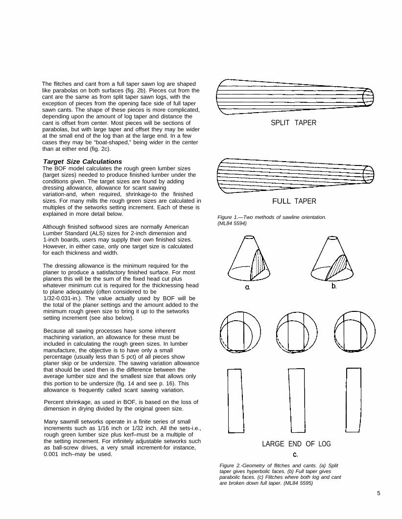
The shape of flitches and cants is calculated from thegeometry of passing cutting planes through a truncated cone(fig. 1). In split taper sawing parallel to the log centerline, theflitches and cant are the shape of a hyperbola on both faces(fig. 2a). Pieces cut from the full length of the cant arerectangles, Those from the taper are also hyperbolas, butwith the sides cut off by lines parallel to the centerline if thecant is sawn split taper. If the cant is sawn full taper, thefull-length pieces are still rectangles while the pieces fromthe taper are shaped like parabolas with the sides cut off(fig. 2b).

4

The flitches and cant from a full taper sawn log are shapedlike parabolas on both surfaces (fig. 2b). Pieces cut from thecant are the same as from split taper sawn logs, with theexception of pieces from the opening face side of full tapersawn cants. The shape of these pieces is more complicated,depending upon the amount of log taper and distance thecant is offset from center. Most pieces will be sections ofparabolas, but with large taper and offset they may be widerat the small end of the log than at the large end. In a fewcases they may be “boat-shaped,” being wider in the centerthan at either end (fig. 2c).

Target Size CalculationsThe BOF model calculates the rough green lumber sizes(target sizes) needed to produce finished lumber under theconditions given. The target sizes are found by addingdressing allowance, allowance for scant sawingvariation-and, when required, shrinkage-to the finishedsizes. For many mills the rough green sizes are calculated inmultiples of the setworks setting increment. Each of these isexplained in more detail below.

Although finished softwood sizes are normally AmericanLumber Standard (ALS) sizes for 2-inch dimension and1-inch boards, users may supply their own finished sizes.However, in either case, only one target size is calculatedfor each thickness and width.

The dressing allowance is the minimum required for theplaner to produce a satisfactory finished surface. For mostplaners this will be the sum of the fixed head cut pluswhatever minimum cut is required for the thicknessing headto plane adequately (often considered to be1/32-0.031-in.). The value actually used by BOF will bethe total of the planer settings and the amount added to theminimum rough green size to bring it up to the setworkssetting increment (see also below).

Because all sawing processes have some inherentmachining variation, an allowance for these must beincluded in calculating the rough green sizes. In lumbermanufacture, the objective is to have only a smallpercentage (usually less than 5 pct) of all pieces showplaner skip or be undersize. The sawing variation allowancethat should be used then is the difference between theaverage lumber size and the smallest size that allows onlythis portion to be undersize (fig. 14 and see p. 16). Thisallowance is frequently called scant sawing variation.

Percent shrinkage, as used in BOF, is based on the loss ofdimension in drying divided by the original green size.

Many sawmill setworks operate in a finite series of smallincrements such as 1/16 inch or 1/32 inch. All the sets-i.e.,rough green lumber size plus kerf–must be a multiple ofthe setting increment. For infinitely adjustable setworks suchas ball-screw drives, a very small increment-for instance,0.001 inch–may be used.

SPLIT TAPER

FULL TAPER

Figure 1.—Two methods of sawline orientation.(ML84 5594)

LARGE END OF LOG

Figure 2.-Geometry of flitches and cants. (a) Splittaper gives hyperbolic faces. (b) Full taper givesparabolic faces. (c) Flitches where both log and cantare broken down full taper. (ML84 5595)

5

Lumber SizesEither one or two lumber thicknesses, nominally 1 inch and2 inches, are used by the BOF model. The log may be sawninto all 1-inch, all 2-inch, or a mixture of the two. If bothsizes are being sawn, the 1-inch is considered a salvagesize and recovered only from the opening cuts on the log orcant.

Five nominal widths–4, 6, 8, 10, and 12 inches-arerequired for use with BOF. In addition, 3-inch lumber may besalvaged, but 3-inch cants will not be produced. At least thefive primary widths must be used when sawing only onethickness. They must also be used with the 2-inch thicknesswhen recovering both 1-inch and 2-inch lumber. In this lattercase, one or more widths of 1-inch lumber may besuppressed.

For mills that do not manufacture five widths, the standardpractice is to rip wide flitches into two or more narrowpieces. Because BOF requires at least five widths, targetsizes that are a combination of several smaller ones areused instead. For example, a mill that does not save2 x 12’s would instead rip a 12-inch flitch into three 2 x 4’s,two 2 x 6’s, or a 2 x 4 and a 2 x 8.

WaneOn finished lumber, up to 25 percent of the thickness andwidth may be wane. This amount is the limit allowed forStandard and Better light framing lumber. To make thecalculations simpler, the wane is based on the greenfinished size. As shrinkage in drying can be assumed to beeven across the piece, the percent of wane on the dryfinished size will not change.

Both the faces and edges of the pieces are checked toensure neither contains excessive wane.

Yield MaximizationThe BOF model can maximize either lumber value or boardfoot volume. In general, value maximization will result in amore profitable and marketable product mix, but volumemaximization will yield a higher lumber recovery.

Value Maximization In maximizing value, net salesreturn-i.e., selling price minus differential conversioncosts-should be used rather than list selling price. Thisapproach avoids bias toward products that have high sellingprices and high production costs. For most mills, the listprice adequately represents the selling price for all products,no matter what volume is produced. Other mills have a fewitems that command a very high selling price, but have verylow demand for the product. In this case, the concept ofvolume discounted prices should be used to determine theselling price. The volume discounted price is the selling priceat which extremely large volumes of each product could bemoved or the selling price minus the cost of holding theseitems in inventory until sold. This concept avoids theproblem of BOF theoretically producing excessive amountsof high-priced product that cannot be sold.

Differential conversion costs for each product size are notusually kept in sawmill accounting systems. However, thesecosts may be calculated knowing the average cost perthousand board feet of lumber in each production area ofthe mill, the total board footage of each size produced, andthe product dimensions.

Green end conversion costs are relatively fixed in the shortterm, no matter what product mix is made. Whether logs arecut heavy to 2 x 4’s or to 2 x 12’s, the crew size remainsthe same, and other operating costs such as power andoperating supplies change very little. Thus, the same greenend cost per thousand board feet may be used for allproducts.

At the dry kiln, planer mill, and shipping departmentsconversion costs will vary among different products basedon number of pieces or lineal feet in a thousand board feetof lumber.

Drying time is shorter for 1-inch lumber than 2-inch, but theboard foot volume of 1-inch lumber that fits in a kiln chargeis less because of sticker spacing. The kiln costs perthousand board feet, then, can be weighted between 1-inchand 2-inch lumber based on kiln capacity and drying time.

Planer production is limited by the lineal feet of lumberpassing through the machine in a given period of time. Forexample, because a thousand board feet of 2 x 4’s containthree times the lineal footage of a thousand board feet of2 x 12’s the planing costs would be three times higher.Further, thin, narrow pieces cause difficulty in manufactureby jamming or breaking up in the planer, so they should beassigned a higher cost.

Dry storage, packing, and shipping costs are directly relatedto the number of pieces in a thousand board feet of lumberand can be allocated on this basis. A few operations maydepend on lineal footage, so this should be consideredwhere appropriate.

As an alternative to using net sales value, a system ofassigning comparative values may be used. These valuesshould reflect the relative net worth of each produced to themill. Using this system, one product, say a 2 x 4, 8 feetlong, is considered the base and assigned an arbitraryvalue, such as 100. All other products are ranked by theirvalue relative to the base. For instance, a very slow movingor difficult to manufacture size may be ranked 50, while ahighly profitable or desirable one could be 200.

The use of comparative values is quicker and requires lesscomputation than compiling net sales returns. However,because these values are arbitrary, more skill andknowledge of the mill’s production and sales are required ifthey are to be used effectively.

6

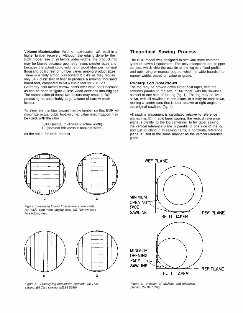
Volume Maximization Volume maximization will result in ahigher lumber recovery. Although the edging done by theBOF model (see p. 9) favors wider widths, the product mixmay be biased because geometry favors smaller sizes andbecause the actual cubic volume of wood fiber per nominalthousand board feet of lumber varies among product sizes.There is a fairly strong bias toward 2 x 4’s as they requireonly 54.7 cubic feet of fiber to produce a nominal thousandboard feet, compared to 58.6 cubic feet for 2 x 12’s.Geometry also favors narrow cants over wide ones because,as can be seen in figure 3, less wood develops into edgings.The combination of these two factors may result in BOFproducing an undesirably large volume of narrow widthlumber.

To eliminate this bias toward narrow lumber so that BOF willmaximize actual cubic foot volume, value maximization maybe used, with the ratio

1,000 (actual thickness x actual width)12 (nominal thickness x nominal width)

as the value for each product.

Figure 3.—Edging losses from different size cants.(a) Wide cant-more edging loss. (b) Narrow cant–less edging loss.

Figure 4.—Primary log breakdown methods. (a) Livesawing. (b) Cant sawing. (ML84 5596)

Theoretical Sawing Process

The BOF model was designed to simulate most commontypes of sawmill equipment. The only exceptions are chippercanters, which chip the outside of the log to a fixed profile,and optimizing or manual edgers, which rip wide boards intonarrow widths based on value or grade.

Primary Log BreakdownThe log may be broken down either split taper, with thesawlines parallel to the pith, or full taper, with the sawlinesparallel to one side of the log (fig. 1). The log may be livesawn, with all sawlines in one plane, or it may be cant sawn,making a center cant that is later resawn at right angles tothe original sawlines (fig. 4).

All sawline placement is calculated relative to referenceplanes (fig. 5). In split taper sawing, the vertical referenceplane is parallel to the log centerline. In full taper sawing,the vertical reference plane is parallel to one side of the logand just touching it. In sawing cants, a horizontal referenceplane is used in the same manner as the vertical referenceplane.

Figure 5.—Relation of sawlines and referenceplanes. (ML84 5597)

The BOF model can simulate sawing systems capable ofplacing the log in any position without regard to a fixedreference line, called variable opening face sawing.Alternatively, BOF can simulate systems in which the log ispositioned with reference to the centerline of the system,called offset sawing (see also p. 19). The first opening facetried is calculated differently depending upon the sawingsystem being modeled.

For variable opening face sawing, the first opening face triedon the log is the one making the shortest, narrowest piece oflumber allowed with maximum wane. If two thicknesses arerecovered, the first piece off the opening face is always thesmaller thickness.

For offset sawing, the position of the first opening face triedis determined by calculating the maximum allowable offset.The center flitch in live sawing, or the cant in cant sawing, isshifted toward the opening face by the maximum offset. Thenumber of thicker pieces that will fit between the centerpiece and the minimum opening face are determined, andthe actual opening face distance is calculated (fig. 6). If athinner piece will also fit, the opening face is further movedout to accommodate this piece.

Successive sawlines are placed across the log until one fallswithin a predetermined distance from the center. Then themodel skips across the cant, or center flitch, and continuesplacing sawlines on the opposite side.

The greatest amount the cant or center flitch may be offsetis one-half the thickness of the thickest piece plus one-halfof a sawkerf. In live sawing, a centered sawline will result atone extreme of offset and a centered flitch at the other.

After the log has been broken down using the first openingface, the opening face is moved towards the center of thelog in variable opening face sawing. In offset sawing, thecant is shifted to the right, and the distance to the openingface is recalculated. The sawing process is then repeated.

This is continued until all allowable opening faces or offsetshave been simulated. The distance the sawing pattern canbe shifted is the smaller of the maximum allowable offset orthe thickness of the thickest piece plus a kerf. The latterrestriction stops the program when the slab contains ausable piece, and the sawing pattern repeats itself.

The distance the sawing pattern is shifted each time(opening face or offset increment) should generally be thesame as the saw setting increment. However, when thesetworks are capable of 0.001-inch accuracy, this smallopening face increment would require large amounts ofcomputer running time. In this case, a compromise betweencomputer time and modeling accuracy can be made byusing a larger opening face increment such as 0.025 inch.

The cant placement and total number of sidepieces may berestricted if necessary to simulate the equipmentconfiguration of a particular mill. For example, somechain-feed multiple bandsaw systems require 4-inch cants tobe centered to avoid sets that would run the saws into thefeed chain, while wider cants may be offset. This situationcan be simulated by the BOF model.

Some mills with multiple saw headsaws cannot resawsidepieces in the same plane as the headsaw. Therefore,they are limited to a cant and as many additional lines asthere are additional saws or chipper heads. Examples aretwo sidepieces for a quad bandsaw or for a twin bandsawwith slab chippers, four for a quad bandsaw with chippers,and none for a chipper canter without saws. To simulatethese conditions, the BOF model allows the number ofsidepieces to be limited. BOF only checks the total numberof sidepieces and, in rare instances, may find a solutioncontaining a different number of sidepieces on each side ofthe cant-for example, two boards on one side and none onthe other. If this situation occurs in a critical application,such as calculating sets for an automated control system, itcan easily be corrected by rerunning those few logs with theallowed number of offsets limited to force a more centeredpattern.

Figure 6.—Determining initial opening face for offsetsawing. (ML84 5598)

Edging and Trimming IndexFlitches are edged parallel to a line joining the wane edge atone side of the large end of the flitch with the wane edge atthe end of the longest piece of lumber (fig. 7). This mostclosely simulates edging with laser lines and provides thegreatest yield.

The BOF model uses one of two edging methods. Infull-length edging, the widest possible full-length board, orpair of boards if the flitch is wide enough, is cut from theflitch. If possible, a piece of the narrowest width is then cutfrom the remaining triangle, and the value and/or volume ofthe pieces is determined (fig. 7). This method simulates theusual situation in which the edger operator cuts the widestfull-length piece possible.

In trim-back edging, the full-length flitch is tested as infull-length edging. Then the flitch is trimmed back 2 feet anda new edging solution found. The flitch is progressivelytrimmed back in 2-foot increments and the solution with thehighest yields is saved. As in full-length edging, a narrowpiece is salvaged if possible. For example, a flitch edged fulllength would yield a 2 x 6, 16 feet long (fig. 8). To determinethe maximum yield of this flitch the model trims the flitchback 2 feet and edges the resulting pieces according to thewane rules. It then calculates the volume and/or value forthis piece. This process is continued until the shortest pieceallowed is processed. The piece that gives the highestvolume or the highest value is then selected. In this case thebest solution is a 2 x 8, 14 feet long. It contains 2-2/3 moreboard feet and is worth more than any other piece. In somecases in which value maximizing is used, a piece with ahigher value but a lower volume will be chosen. In thisexample, a 2 x 6, 16 feet long, has less volume but is worthmore than a 2 x 10, 10 feet long.

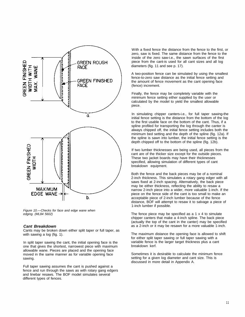
In determining which widths can be cut from a flitch, bothedging methods use a precalculated array containing theface and edge, with and without wane, required for eachallowable edging combination. The flitch is checked toensure it meets the allowance for both face and edge wane.The piece of lumber is assumed to be centered in thethickness of the flitch. For the lumber to fit, the flitch must bewider than the width required by that product size withmaximum wane (fig. 10). For example, to cut a finished2 x 4, 3-1/2 inches wide, assuming 5 percent shrinkage, and25 percent wane, the flitch must be at least

Two pieces may be produced from flitches wider than 12inches. When two pieces will fit in a flitch, the wider piece isalways the longer-for example, a flitch, which, when edgedfull length, yields a 2 x 12, 16 feet long, can also better beedged to yield a 2 x 10, 16 feet long, and a 2 x 4, 10 feetlong (fig. 9). As before, the model tries the full-length andsuccessively shorter pieces in the flitch and finds the onethat gives the best yield. This method simulates a simpleautomated optimizing edger when only combinations basedon the widest pieces are cut. The combinations used in BOFedging are as follows:

wide on the green finished face of the lumber. At the point ofmaximum allowable edge wane that flitch must be widerthan the green finished lumber size. This point is inside thegreen finished face a distance that can be found bymultiplying the edge wane factor by the green finishedthickness. In live sawing, the wane on the center flitch ischecked on the side farthest from the center of the log.

Nominal widths

Figure 7.—Full-length edging method. (ML84 5599)

9

Figure 8.—Trim back edging method-narrow pieces. (ML84 5600)

Figure 9.—Trim back edging method-wide pieces. (ML84 5601)

10

Figure 10.—Checks for face and edge wane whenedging. (ML84 5602)

Cant BreakdownCants may be broken down either split taper or full taper, aswith sawing a log (fig. 1).

In split taper sawing the cant, the initial opening face is theone that gives the shortest, narrowest piece with maximumallowable wane. Pieces are placed and the opening facemoved in the same manner as for variable opening facesawing.

Full taper sawing assumes the cant is pushed against afence and run through the saws as with rotary gang edgersand linebar resaws. The BOF model simulates severaldifferent types of fences.

With a fixed fence the distance from the fence to the first, orzero, saw is fixed. The same distance from the fence to theinside of the zero saw-i.e., the sawn surfaces of the firstpiece from the cant-is used for all cant sizes and all logdiameters (fig. 11 and see p. 17).

A two-position fence can be simulated by using the smallestfence-to-zero saw distance as the initial fence setting andthe amount of fence movement as the cant opening face(fence) increment.

Finally, the fence may be completely variable with theminimum fence setting either supplied by the user orcalculated by the model to yield the smallest allowablepiece.

In simulating chipper canters-i.e., for full taper sawing-theinitial fence setting is the distance from the bottom of the logto the first usable face on the bottom of the cant. Thus, if aspline profiled for transporting the log through the canter isalways chipped off, the initial fence setting includes both theminimum bed setting and the depth of the spline (fig. 12a). Ifthe spline is sawn into lumber, the initial fence setting is thedepth chipped off to the bottom of the spline (fig. 12b).

If two lumber thicknesses are being used, all pieces from thecant are of the thicker size except for the outside pieces.These two jacket boards may have their thicknessesspecified, allowing simulation of different types of cantbreakdown equipment.

Both the fence and the back pieces may be of a nominal2-inch thickness. This simulates a rotary gang edger with allsaws fixed at 2-inch spacing. Alternatively, the back piecemay be either thickness, reflecting the ability to resaw anarrow 2-inch piece into a wider, more valuable 1-inch. If thepiece on the fence side of the cant is too small to make anacceptable piece of 2-inch lumber because of the fencedistance, BOF will attempt to resaw it to salvage a piece of1-inch lumber if possible.

The fence piece may be specified as a 1 x 4 to simulatechipper canters that make a 4-inch spline. The back piece(actually the top of the cant in the canter) may be specifiedas a 2-inch or it may be resawn for a more valuable 1-inch.

The maximum distance the opening face is allowed to shiftfor either split taper sawing or full taper sawing with avariable fence is the larger target thickness plus a cantbreakdown kerf.

Sometimes it is desirable to calculate the minimum fencesetting for a given log diameter and cant size. This isdiscussed in more detail in Appendix A.

11

Figure 11.—Relation of fence setting distance andfirst face on cant. (ML84 5603)

In cant sawing, the solution giving the highest yield is foundby calculating solutions using all five cant sizes (4, 6, 8, 10,and 12 in.). In some circumstances, however, it may benecessary to limit the production of some lumber widths orto reduce computer running time. Both of these can beaccomplished by limiting the number of cant sizes used. Inaddition, equipment limitations may prevent manufacture ofsome cants, as in a mill where the only cant breakdownmachine is a 6-inch rotary gang edger. To simulate thiscase, BOF can be instructed not to make 8-, 10-, or 12-inchcants. Any cant size may be suppressed to reduceproduction of that size.

For maximizing volume, the model can be directed to cut thelargest cant size possible. This forces the production ofwider-width lumber. A side effect is the loss of recoverywhen wide cants are cut from small logs. This particularrecovery loss can be minimized by specifying the smallestdiameter log from which a particular cant size may be cut.Increasing the smallest acceptable diameter log to one thatyields a cant and two side pieces will provide a balancebetween the advantages of cutting the widest cant and therecovery losses associated with small logs.

A similar means of restricting the cants is available formaximizing value. The program ranks the cants by anefficiency factor reflecting the actual wood used to saw eachcant size and the value of each length. This factor is:

Efficiency factor = nominal cant thicknessactual cant thickness + headsaw kerf

The weighted value of each cant size and length iscalculated by:

Weighted value = efficiency factor x value/MBF

Thus, if less actual wood is used for a given nominal size,that size is relatively more valuable. Within each length, thecants are ranked in order of highest weighted value. Forexample (table 1), a 6-inch cant is nominally more valuablethan a 4-inch cant. However, when wood-use efficiency isconsidered, the 4-inch cant is more valuable and should beused.

In sawing each log, the model selects the highest rankedcant size that will fit in the log. For the example in table 2,BOF will select 12-inch cants for all logs large enough. Thesecond choice would be a 10-inch cant. For 8-, 10-, and16-foot logs too small to fit a 10-inch cant, a 4-inch cantwould always be cut. No 8-, 10-, 16-foot, 6-, or 8-inch cantswould be cut using this ranking table. The 12- and 14-footlogs would be cut with an 8-inch cant if too small for a 10, a6-inch cant if too small for an 8, and finally a 4-inch cant iftoo small for a 6.

Figure 12.—Determining fence setting distance whensimulating chipper canters. (a) Spline is alwayschipped off. (b) Spline is made into lumber.(ML85 5604)

12

Using the Best Opening Face Program

Yield MaximizationAfter the log has been theoretically sawn using eachopening face, the volume or value of the resulting solution iscompared to that of the previously saved best solution, andthe larger of the two is saved. Only the volume or value, ifapplicable, and offset of the center piece are saved for eachsuccessive best solution. After all allowable opening faceshave been tried and the best solution found, the log is sawnonce more using the best opening face, and this solution isprinted.

If a number of consecutive opening faces all have the samemaximum yield, the sawing solution printed will be the oneclosest to the center of the range. This approach was takenbecause, in using the BOF model to calculate sets forautomated sawing systems, it provides the widest latitude inpositioning the log to recover the maximum yield.

In maximizing value, an occasional anomaly can occur in theprintout in which the total lumber volume does not equal thesum of the individual pieces. Because the lumber volumeprinted is saved from the last solution within the range andthe pieces printed are from the solution in the center of therange, the two solutions may not equal each other if madeup of differing product mixes.

The sawmill configuration simulated by BOF is controlled bydata describing a particular mill and options that control theprogram flow. Those interested in modifying the program orin getting a better understanding of how the data are usedcan obtain a FORTRAN listing of BOF from State andPrivate Forestry, Madison, WI. Certain information isrequired and must be supplied. Other information has defaultvalues that may be overridden.

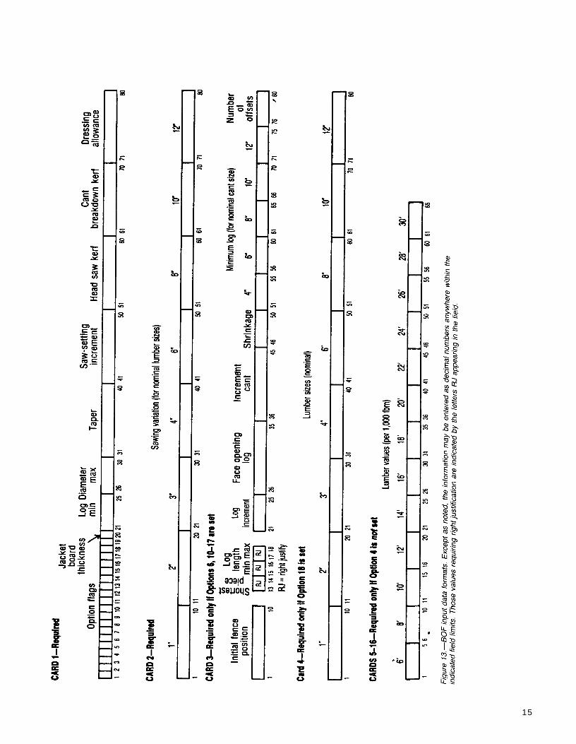
Table 3 summarizes the options available and theinformation required for using BOF. The necessary datacards are illustrated in figure 13. The first two cards containinformation that changes from mill to mill and allows variousprocessing options to be selected.

Required Information

Minimum and Maximum Small-End LogDiameterThe minimum small-end log diameter should be no smallerthan will produce one piece of the smallest size lumber.However, if a smaller log is specified, the program willcalculate the minimum diameter and skip any logs that aretoo small. The maximum small-end log diameter is limitedpartly by the widest flitch the program can edge. This flitchcontains two 2 x 12’s and one salvage piece of thenarrowest width specified, either a 2 x 4 or 2 x 3. The limitalso depends on the sawing method, maximum log length,and amount of taper. For live sawing long logs withappreciable taper, the maximum diameter should not exceed21 inches. When cant sawing short, low-taper logs andrecovering the widest cant, the upper limit is about28 inches. Because the program does not check for verylarge logs, some flitches from logs exceeding these units willnot be edged correctly, and the yield will be underestimated.

TaperTaper is the difference between the large- and small-enddiameters of a log. It is entered as decimal inches per16 feet of log length.

Saw Setting IncrementSaw setting increment is the minimum amount by which thesetworks move a log with respect to the saws. For setworksthat move in finite steps, such as hydraulic stack cylinders,this increment should be used. For continuously adjustablesetworks, such as ball-screw setworks, a smallincrement-e.g., 0.001 inch-should be used.

13

14

15

Headsaw KerfHeadsaw kerf is the kerf width of the first saw used to breakdown the log. In many cases, such as twin and quadbandsaw headrigs, several saws are involved, but all havethe same kerf and saw the log in parallel planes generallyconsidered to be vertical (fig. 4). If standard mill practice isto take a minimal number of lines at the headsaw, produceflitches that contain multiple pieces, and further break theseflitches down in the same plane on another saw with adifferent kerf, the weighted average of the two kerfs shouldbe entered. This will introduce a small amount of error, butin most cases it will not be as significant as if only one kerfvalue were used.

Cant Breakdown KerfCant breakdown kerf is the kerf width of the saw or sawsused to break down the cant and is also used as the kerf foredging flitches. If different kerf widths are used for cantbreakdown and for board edging, the cant breakdown kerfshould be used as this normally covers a larger volume oflumber. The sawlines in the cant are perpendicular to thesawlines in the log and are generally considered to behorizontal (see option 2 on p. 17 and fig. 4). If two or morecant breakdown machines are used interchangeably, theirkerfs should be pro-rated.

Dressing AllowanceDressing allowance is the additional thickness or widthdimension necessary to obtain a satisfactory dressedsurface on finished lumber. It is determined by adding thecut of the fixed planer head to the minimum cut (oftenconsidered to be 1/32 in.) required by the thicknessing headto obtain a satisfactory finish. For example, a fixed head cutof 0.062 inch plus minimum cut for thicknessing head of0.031 inch means 0.093 is used. If the lumber is not to bedressed, a very small value such as 0.000001 should beused.

Sawing VariationSawing variation is an expression of the sizing variationabove (+) and below (-) the average target thickness orwidth of lumber. In determining the required target size forrough green lumber an allowance for the scant or negativesawing variation must be made. Figure 14 shows what scantsawing variation is and how it can be determined. Forexample, if the average target size of nominal 4-inch is3.950 and 95 percent of the 4-inch pieces are found to bethicker than 3.750, then the scant sawing variation is 0.200.The scant sawing variation is added to the minimum roughgreen size to determine the necessary average target size tostay within a prescribed sizing tolerance–e.g., 95 percent.

Figure 14.—Scant sawing variation is the difference between the average rough green lumber size and95 percent of the low end of the total sawing variation. (ML84 5605)

16

Program Control Options

BOF can be made to simulate individual mill configurationsby specifying various options and entering supplementaryinformation where necessary. These options are set byentering values in the appropriate columns of the first card.If an option is not set, either a blank or 0 (zero) may beentered. Options should be set by entering a 1 unlessotherwise specified under the individual option.

Option 1. Processing Control

Not set: The program is run and the solutions are output.

Set: Enter 1. The input information will be listed, but theindividual log solutions will not be calculated. This allows theuser to check the accuracy of the input data without actuallycalculating the BOF solutions

Enter 9. A 9 tells the BOF program that all data have beenrun and processing should be terminated. If more than oneset of data are to be run, the last data card of one setshould be immediately followed by the first card of the nextset. Whether one data set or multiple sets are run, the lastcard should contain a 9 in column 1 to terminate processing.

Option 2. Sawing Method (fig. 4)

Not set: The cant sawing method will be used. A center cantand side lumber will be produced in the “vertical” plane. Thecant is then further broken down by sawlines in the“horizontal” plane.

Set: The live sawing method will be used. All log breakdownlines are in the vertical plane.

Option 3. Lumber Sizes

Not set: The finished sizes are assumed to be dry, andshrinkage will be considered in calculation of target sizes.The shrinkage percentage is controlled by Option 15.

Set: The finished sizes are assumed to be green, andshrinkage is not considered.

Option 4. Yield Maximization

Not set: BOF calculates the solutions yielding the greatestvalues. These may or may not be the highest volumesolutions. Values per thousand board feet are used for eachlumber size and length being cut. The number of valuesused depends on the jacket board thickness (Option 20) andthe narrowest piece allowed (Option 10). Values for alllengths for each lumber size are entered on one card. Foreach thickness the values are entered in order of increasingwidth. If two thicknesses are cut, the value cards for the1-inch thickness are entered first, followed by those for the2-inch thickness (see fig. 13). If both 1-inch and 2-inchlumber are cut and certain sizes of 1-inch lumber are notdesired, these may be suppressed by entering a very smallvalue such as 0.10 per thousand board foot for those sizes.

Note that 2-inch lumber and 1 x 4’s, when Option 6 is setwith 1 or 3, SHOULD NOT be suppressed in this way. Inaddition, when only one thickness is used no lumber shouldbe suppressed.

Set: BOF calculates solutions yielding the greatest nominalboard foot volumes. They may or may not be the highestvalues.

Option 5. Cant Sawing Maximization Method (usedonly if cant sawing-i.e., Option 2–is not set)

Not set: (a) Option 4 not set. The cant with the highestweighted value that can be cut from the log will be used.(See p. 12 for explanation of “weighted” value.)(b) Option 4 set. The largest cant that can be cut from thelog will be used. Either BOF will calculate the smallest logdiameter in which a given cant size will fit, or the user mayspecify the smallest diameter to be used. This is defined byOption 16.

Set: Enter 1. The largest cant that can be cut from the logwill be used. Note that if Option 4 is set, this has no effect.

Enter 5. Solutions will be calculated for all possible cantsizes that can be sawn from the log, and the one giving thehighest total volume or value yield will be chosen.

Option 6. Cant Breakdown Method (used only if cantsawing–i.e., Option 2–is not set) (fig. 1)

Not set: Split taper. The sawlines will be parallel to thecenterline of the cant.

Set: Full taper. The sawlines in the cant will be parallel toone of the unsawn faces–i.e., when using a fence.

Enter 1. A 1 x 4 is taken from the fence side of the cant, a1- or 2-inch on the back. Even if the cant is wider, only a1 x 4 will be taken on the fence side.

Enter 2. A 2-inch piece will be taken from the fence side, a1- or 2-inch on the back.

Enter 3. A 1 x 4 will be taken from the fence side of cant, a2-inch on the back.

Enter 4. A 2-inch piece will be taken from the fence sideand a 2-inch on the back.

Option 7. Cant Breakdown Fence (full taper cantsawing-i.e., Options 2 and 6 set)

The initial fence position is the distance from where the sideof the cant touches the fence to the first usable face of thecant (figs. 11 and 12).

Not set: The fence position is fixed, and the same distancewill be used for all cant sizes. The fence position must beentered on card 3.

17

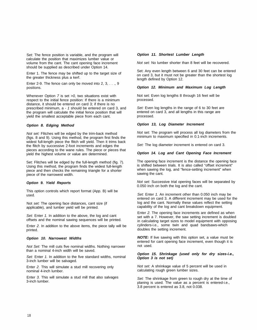
Set: The fence position is variable, and the program willcalculate the position that maximizes lumber value orvolume from the cant. The cant opening face incrementshould be supplied as described under Option 14.

Enter 1. The fence may be shifted up to the target size ofthe greater thickness plus a kerf.

Enter 2-9. The fence can only be moved into 2, 3, . . ., 9positions.

Whenever Option 7 is set >0, two situations exist withrespect to the initial fence position: If there is a minimumdistance, it should be entered on card 3; if there is noprescribed minimum, a - 1 should be entered on card 3, andthe program will calculate the initial fence position that willyield the smallest acceptable piece from each cant.

Option 8. Edging Method

Not set: Flitches will be edged by the trim-back method(figs. 8 and 9). Using this method, the program first finds thewidest full-length piece the flitch will yield. Then it trims backthe flitch by successive 2-foot increments and edges thepieces according to the wane rules. The piece or pieces thatyield the highest volume or value are determined.

Set: Flitches will be edged by the full-length method (fig. 7).Using this method, the program finds the widest full-lengthpiece and then checks the remaining triangle for a shorterpiece of the narrowest width.

Option 9. Yield Reports

This option controls which report format (App. B) will beused.

Not set: The opening face distances, cant size (ifapplicable), and lumber yield will be printed.

Set: Enter 1. In addition to the above, the log and cantoffsets and the nominal sawing sequences will be printed.

Enter 2. In addition to the above items, the piece tally will beprinted.

Option 10. Narrowest Widths

Not Set: The mill cuts five nominal widths. Nothing narrowerthan a nominal 4-inch width will be saved.

Set: Enter 1. In addition to the five standard widths, nominal3-inch lumber will be salvaged.

Enter 2. This will simulate a stud mill recovering onlynominal 4-inch lumber.

Enter 3. This will simulate a stud mill that also salvages3-inch lumber.

Option 11. Shortest Lumber Length

Not set: No lumber shorter than 8 feet will be recovered.

Set: Any even length between 6 and 30 feet can be enteredon card 3, but it must not be greater than the shortest loglength defined by Option 12.

Option 12. Minimum and Maximum Log Length

Not set: Even log lengths 8 through 16 feet will beprocessed.

Set: Even log lengths in the range of 6 to 30 feet areentered on card 3, and all lengths in this range areprocessed.

Option 13, Log Diameter Increment

Not set: The program will process all log diameters from theminimum to maximum specified in 0.1-inch increments.

Set: The log diameter increment is entered on card 3.

Option 14. Log and Cant Opening Face Increment

The opening face increment is the distance the opening faceis shifted between trials. It is also called “offset increment”when sawing the log, and “fence-setting increment” whensawing the cant.

Not set: Successive trial opening faces will be separated by0.050 inch on both the log and the cant.

Set: Enter 1. An increment other than 0.050 inch may beentered on card 3. A different increment may be used for thelog and the cant. Normally these values reflect the settingcapability of the log and cant breakdown equipment.

Enter 2. The opening face increments are defined as whenset with a 7. However, the saw setting increment is doubledin calculating target sizes to model equipment with opposingcylinders-i.e., some twin and quad bandsaws-whichdoubles the setting increment.

NOTE: If live sawing with this option set, a value must beentered for cant opening face increment, even though it isnot used.

Option 15. Shrinkage (used only for dry sizes-i.e.,Option 3 is not set)

Not set: A shrinkage value of 5 percent will be used incalculating rough green lumber sizes.

Set: The shrinkage from green to rough dry at the time ofplaning is used. The value as a percent is entered-i.e.,3.8 percent is entered as 3.8, not 0.038.

18

Option 16. Minimum Log Required for a Cant

Not set: The program will calculate the minimum logdiameter that will produce a cant containing one of thefollowing: two 2 x 4’s, two 2 x 6’s, three 2 x 8’s, three2 x 10’s, or three 2 x 12’s.

Set: When set >0, for each cant size the user can, oncard 3, specify the minimum log diameter required, candirect the program to calculate the minimum log diameter, orcan suppress the cant size.

(a) The minimum log diameter from which the cant size willbe recovered can be entered. This diameter must be largeenough to recover at least one piece of lumber the width ofthe cant.

(b) If a 0 (zero) is entered, the program will calculate theminimum log diameter for that cant size, as if Option 16were not set.

(c) If a - 1 is entered, the program will ignore that cant size.

(d) If 30 or greater is entered, that cant size and any largercant sizes will be ignored. This option should be used tosuppress cants larger than largest desired size, while (c)should be used to suppress those smaller.

Enter 1. Cant sizes will be controlled as described above.

Enter 2, 4, 6, or 8. Cant sizes will be controlled asdescribed above. In addition, the maximum number of sideboards allowed will be 2, 4, 6, or 8.

Enter 9. Cants will be controlled as above. In addition, nosideboards will be produced.

Option 17. Variable Opening Face and OffsetPositions

Not set: Variable opening face sawing. Starting with theopening face yielding the smallest acceptable piece, allopening faces within the limits calculated by the program willbe tried. If two thicknesses are used, the first piece next tothe opening face will always be the smaller thickness.

Set: Offset sawing. This allows the user to specify thenumber of positions to which the log may be shifted off thecenter-line of the system. This number includes the centeredposition and should reflect the mechanical capability of thelog setting equipment. Thus, if the log movement is limitedto the centered position and four offsets, the number ofoffsets entered on card 3 is 5. For center sawing systemswith no offset capability, the number of offsets is 1.

Enter 1. All cant sizes will be offset as limited above.

Enter 2. Nominal 4-inch cants will be centered on the smallend of the log, whereas larger cants will be offset as limitedabove.

Option 18. Lumber Dimensions

Not set: The dressed lumber will be American LumberStandard (ALS) sizes. If Option 3 is not set (dry lumber), theALS dry sizes will be used. If Option 3 is set (green lumber),ALS green sizes will be used.

Set: The user may enter finished sizes on card 4.

When multiple piece sizes are being entered, the followingformulas can be used. For combining two pieces, theequation for calculating the rough dry size is:

or for three pieces, where Size, is the middle:

where

In the above formulas, sawing variation and sawkerf are“shrunken” to bring them down to the dry size as theprogram lumber size calculations will “swell” them up to thegreen size. In the case in which the composite size is madeup of two pieces, the sawing variation is only that on oneside of each piece, while for three pieces, the entirevariation is added in for the middle piece and half the totalvariation for each side piece. When the BOF program is run,the two unused half sawing variations are added andentered as total sawing variation.

These calculations are performed automatically by theprogram if the option is set to run a stud mill with all sizes2 x 4 or smaller.

19

Option 19. Log Breakdown Method (fig. 1)

Not set: Split taper. The log is sawn parallel to thecenterline.

Set: Enter 1. Full taper. The log is sawn parallel to theopening face side.

Enter 2. Both split taper and full taper will be tried and thebest solution printed.

Option 20. Jacket Board and Lumber Thickness

This option must be set.

Enter 1. All lumber will be nominally 1 inch thick.

Enter 2. All lumber will be nominally 2 inches thick.

Enter 3. Primary production will be nominally 2 inches withthe jacket boards on the log and cants 1 or 2 inchesdepending upon Options 17 and 6.

Literature Cited

20

Bibliography of OtherPublications Related toBest Opening Face

21

Appendix ACalculating the MinimumCant Breakdown Fence Setting

For setting up the fence on a rotary gangsaw or other cantbreakdown equipment, it is desirable to have the initialfence-to-zero-saw distance be the smallest possible to allowrecovery of a usable piece from the minimum-diameter log.The formulas below will calculate the setting that will recoverthe narrowest, shortest piece from the fence side of thecant. This piece will have the maximum wane allowed.

In practice, irregularities in log shape will probably result inexcessive wane on pieces from minimum-diameter logs.However, use of these formulas provides a starting point forjudging the best initial fence setting to minimize edgingwaste (fig. Al).

Let:R = log radius at the shortest lumber length from the large

end of the log.F = minimum face width being considered on the fence

side of the cant.D = distance from the center of the log to face F at the

point at which R is determined.W = dry finished width of the smallest allowable piece of

lumber.T = dry finished thickness.S = shrinkage factor.

WA = wane allowance factor.

Step 1. Calculate the distance from the log center to thegreen finished face with maximum wane:

where

Step 2. Calculate the distance from the log center to thegreen finished face allowing maximum edge wane:

where

Step 3. Calculate the distance to the sawn face allowingmaximum wane:

where DR = dressing allowance.SV = sawing variation of thickness, T.

Step 4. The minimum fence setting (FS) is then:

F S = R - D

22

Figure A1.—The larger fence setting will meet bothface and edge wane restrictions. (ML84 5606)

Appendix BBest Opening Face Reports

The following reports are examples of those generated bythe BOF program. Most of the information in them isself-explanatory, but those items that could be ambiguousare explained below.

Report B.1 shows the values used in calculating the roughlumber sizes. Dressing allowance, as printed, contains theminimum dressing allowance and the oversizing needed tocome up to a multiple of the saw setting increment.Shrinkage is the loss from green to dry of the rough lumberand dressing allowance. It does not include sawing variation.

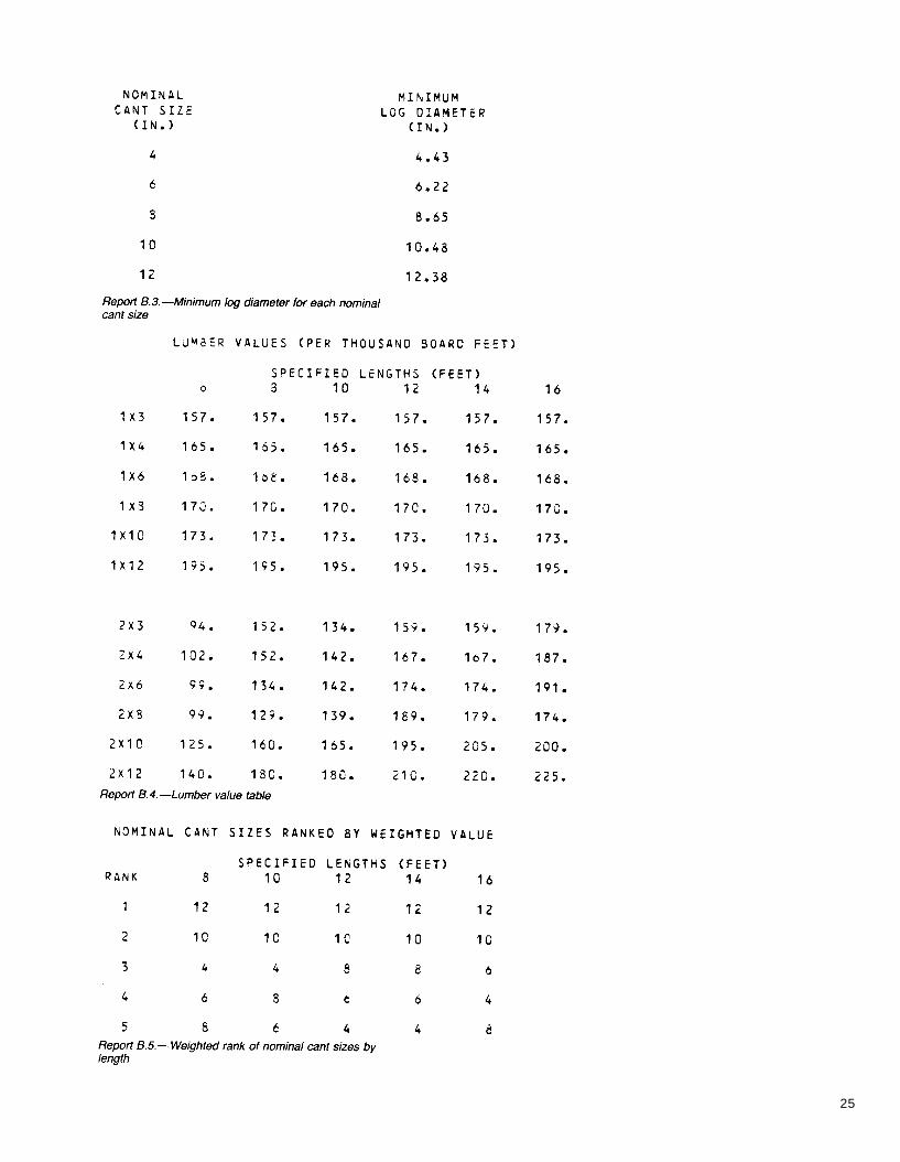
Report B.3 lists the smallest log diameter from which eachcant size can be sawn. Unless the diameter is specified, thelog is large enough to fit a cant containing two 2 x 4’s, two2 x 6’s, three 2 x 8’s, three 2 x 10’s, or three 2 x 12’s.

Report B.5 lists the weighted ranking of each cant size bylength. It is printed only when maximizing value, and whenusing the highest ranked cant. It is not printed whenselecting the largest cant or when testing all cant sizes.Within each length, the highest ranked cant that meets theminimum log diameter restriction will be chosen.

Reports B.6 through B.11 illustrate various levels of detail inpresenting the results of the BOF calculations.

The Best Opening Face distances are from the center ofthe small end of the log to the sawn surface of the outerpieces. Figure B1 shows the locations of these distances.

Range is the number of consecutive opening faces that givethe maximum yield. When the range is an odd number, thesolution printed is based on the opening face in the middleof the range. If range is even, the rightmost of the centertwo opening faces is used. FT or ST next to the range tellswhether the log or cant was sawn full taper or split taper.

Lumber Recovery Factor is the ratio of board feet lumberrecovered divided by the actual cubic foot log volume. Cubicfoot volume is calculated using Smalian’s formula.

Sawing Sequence, shown in Reports B.7, B.8, B.10, andB.11, is the nominal thickness of the sawlines going from theleft opening face to the right opening face. Offset, in thesereports, is the distance the center of the cant or center pieceis shifted off the center of the small end. The shift is to theleft when offset is negative and to the right when offset ispositive.

Fence is shown only when the cant is full taper sawn. It isthe distance from the outside of the log to the sawn surfaceof the cant left opening face.

Figure B1.—Location of opening faces looking at thesmall end of the log, (A) Best Opening Face, distancefrom center, left; (B) cant opening face, distance fromcenter, right; Best Opening Face, distance from center,right; (D) distance, left face to cant; (E) cant openingface, distance from center, left; and (F) fence.(ML84 5607)

23

24

25

26

27

Appendix CConsiderations for Using BestOpening Face to Simulate SawmillsProducing Metric-Sized Lumber

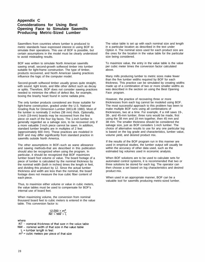
Sawmillers from countries where lumber is produced tometric standards have expressed interest in using BOF tosimulate their operations. This use of BOF is possible, butcertain assumptions in the model must be clearly understoodto avoid misleading results.

BOF was written to simulate North American sawmillssawing small, second-growth softwood timber into lumbersuitable for light-frame construction. The type of timber,products recovered, and North American sawing practicesinfluence the logic of the computer model.

Second-growth softwood timber usually grows quite straight,with sound, tight knots, and little other defect such as decayor splits. Therefore, BOF does not consider sawing practicesneeded to minimize the effect of defect like, for example,boxing the brashy heart found in some radiata pine.

The only lumber products considered are those suitable forlight-frame construction, graded under the U.S. NationalGrading Rule for Dimension Lumber (WCLIB 1980). Most ofthe lumber is nominally 2 inches (38 mm) thick. Optionally,1-inch (19-mm) boards may be recovered from the firstpiece on each of the four log faces. The 1-inch lumber isgenerally regarded as a salvage size, to be recovered only ifa more valuable 2-inch piece cannot be sawn. In addition,standard lumber lengths are in multiples of 2 feet(approximately 600 mm). These practices are modeled inBOF and may differ significantly from standard practice insawmills outside North America.

The other assumptions in BOF–such as wane allowanceand sawing methods-that are described in this publicationshould also be recognized when using the program. Inparticular, it should be recognized that BOF maximizeslumber board foot volume or value. The board footage of apiece of lumber is calculated by the nominal thickness bythe nominal width (both in inches) times the length in feet,and dividing this product by 12. Since the actual lumberthickness and width are less than the nominal, the boardfootage does not measure the true cubic fiber content ofeach piece.

Thus, to maximize either volume or value in cubic meters,the value tables must be used to compensate for BOF’sinternal use of board feet.

When maximizing volume, the conversion from nominalthousand board feet to cubic meters is entered in the valuetable. This conversion factor is:

The value table is set up with each nominal size and lengthin a particular location as described in the text underOption 4. The nominal sizes used for each product size arethe ones for the location in the value table for the particularsize being considered.

To maximize value, the entry in the value table is the valueper cubic meter times the conversion factor calculatedabove.

Many mills producing lumber to metric sizes make fewerthan the five lumber widths required by BOF for eachthickness. This practice can be simulated by creating widthsmade up of a combination of two or more smaller widths aswas described in the section on using the Best OpeningFace program.

However, the practice of recovering three or morethicknesses from each log cannot be modeled using BOF.The most successful approach to this problem has been tomake multiple BOF runs using all combinations ofthicknesses, two at a time. For example, if a mill saws 19-,38-, and 45-mm lumber, three runs would be made, firstusing the 38 mm and 19 mm together, then 45 mm and38 mm. The smaller thickness should be considered thesalvage size, just as BOF considers 1-inch lumber. Thechoice of alternative results to use for any one particular logis based on the log grade and characteristics, lumber value,volume yield, and desired product mix.

If the results of the BOF program run in this manner areused in empirical studies, the lumber output will usually bewithin the accuracy of other data used, such as theestimated log volumes used in economic analysis.

When BOF solutions are to be used to calculate sets forautomated control systems, it is recommended that two orthree solutions be stored for each log. The operator canthen choose a set based on log characteristics and desiredproduct mix.

When used in an appropriate manner, BOF can be avaluable tool for sawmills producing metric-sized lumber.

28

Acknowledgments Program

Simulation models often evolve, with each improvementbeing the result of questions and comments fromknowledgeable people. At times contributions are even moredirect. For their help, I thank my coworkers-particularlyJeanne Danielson, for contributing the appendices and formany useful discussions, ideas, and suggestions, and HiramHallock, now retired, who conceived the idea for and jointlydevelped the original version of BOF.

I would also like to thank the many people in the sawmillindustry and the Forest Service whose questions andcomments on the practical side of sawmilling helped makethe information in this paper possible.

US. GOVERNMENT PRINTING OFFICE. 1987- 7 4 2 - 0 4 4 / 4 0 0 1 5

The FORTRAN source for the BOF program is available inelectronically readable form from:

U.S. Department of Agriculture, Forest ServiceState and Private ForestryOne Gifford Pinchot DriveMadison, WI 53705-2398

It is titled “FORTRAN Listing of the Best Opening FaceSystem.”

1.5-2/86

29