Ahmed H. Qureshi, Yinglong Miao, Anthony Simeonov and ...

Motion Planning Networks: Bridging the Gap BetweenLearning-based and Classical Motion PlannersAhmed H. Qureshi, Yinglong Miao, Anthony Simeonov and Michael C. Yip

Abstract—This paper describes Motion Planning Networks(MPNet)1, a computationally efficient, learning-based neuralplanner for solving motion planning problems. MPNet usesneural networks to learn general near-optimal heuristics forpath planning in seen and unseen environments. It receivesenvironment information as point-clouds, as well as a robot’sinitial and desired goal configurations and recursively calls itselfto bidirectionally generate connectable paths. In addition tofinding directly connectable and near-optimal paths in a singlepass, we show that worst-case theoretical guarantees can beproven if we merge this neural network strategy with classicalsample-based planners in a hybrid approach while still retainingsignificant computational and optimality improvements. To learnthe MPNet models, we present an active continual learningapproach that enables MPNet to learn from streaming data andactively ask for expert demonstrations when needed, drasticallyreducing data for training. We validate MPNet against gold-standard and state-of-the-art planning methods in a variety ofproblems from 2D to 7D robot configuration spaces in challengingand cluttered environments, with results showing significant andconsistently stronger performance metrics, and motivating neuralplanning in general as a modern strategy for solving motionplanning problems efficiently.

I. INTRODUCTION

Motion planning is among the core research problems inrobotics and artificial intelligence. It aims to find a collision-free, low-cost path connecting a start and goal configurationfor an agent [4] [5]. An ideal motion planning algorithmfor solving real-world problems should offer following keyfeatures: i) completeness and optimality guarantees — imply-ing that a solution will be found if one exists and that thesolution will be globally optimal, ii) computational efficiency— finding a solution in either real-time or in sub-second timesor better while being memory efficient, and iii) insensitivityto environment complexity — the algorithm is effective andefficient in finding solutions regardless of the constraints ofthe environment. Decades of research have produced manysignificant milestones for motion planning include resolution-complete planners such artificial potential fields [6], sample-based motion planners such as Rapidly-Exploring RandomTrees (RRT) [4], heuristically biased solvers such as RRT*[1] and lazy search [7]. Many of these developments arehighlighted in the related work section (Section II). However,each planner and their variants have tradeoffs amongst theideal features of motion planners. Thus, no single motionplanner has emerged above all others to solve a broad rangeof problems.

A. H. Qureshi, Y. Miao, A. Simeonov and M. C. Yip are affiliated with Uni-versity of California San Diego, La Jolla, CA 92093 USA. {a1qureshi,y2miao, asimeono, yip}@ucsd.edu

1Supplementary material including implementation parameters and projectvideos are available at https://sites.google.com/view/mpnet/home.

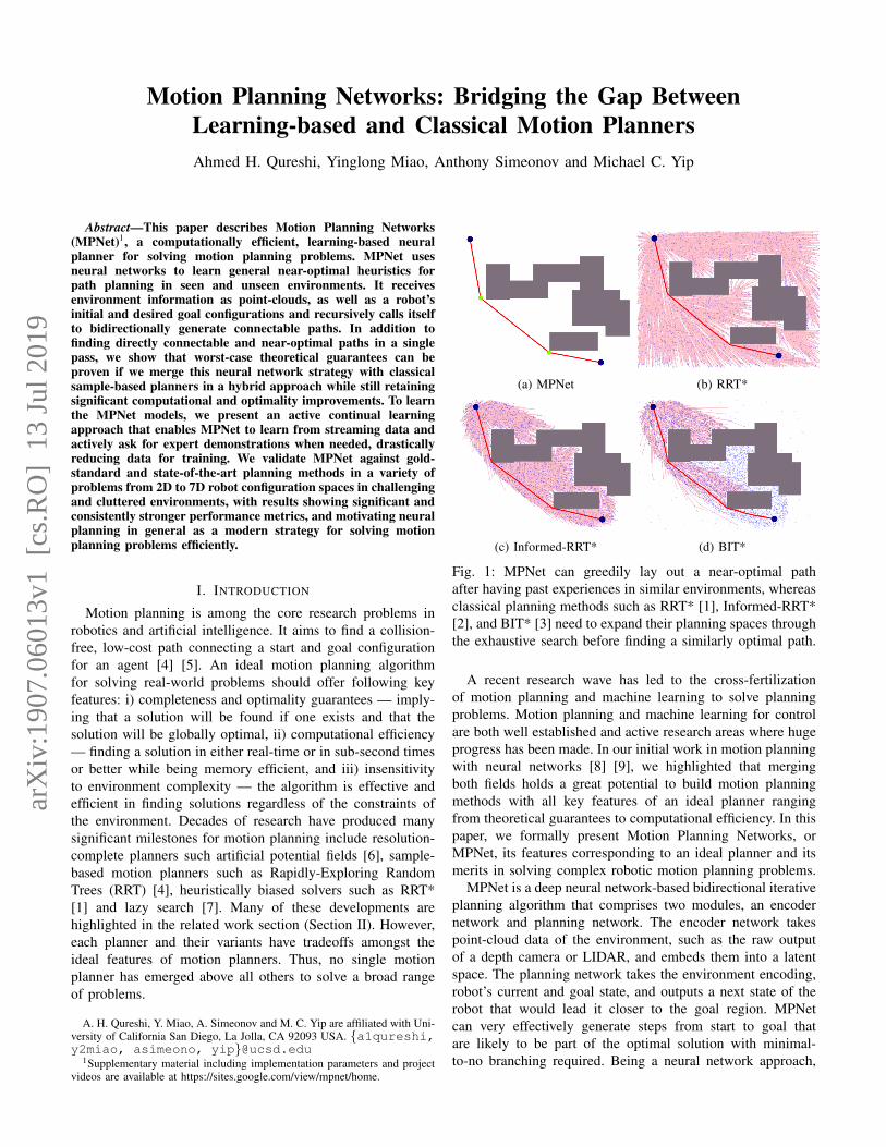
(a) MPNet (b) RRT*

(c) Informed-RRT* (d) BIT*

Fig. 1: MPNet can greedily lay out a near-optimal pathafter having past experiences in similar environments, whereasclassical planning methods such as RRT* [1], Informed-RRT*[2], and BIT* [3] need to expand their planning spaces throughthe exhaustive search before finding a similarly optimal path.

A recent research wave has led to the cross-fertilizationof motion planning and machine learning to solve planningproblems. Motion planning and machine learning for controlare both well established and active research areas where hugeprogress has been made. In our initial work in motion planningwith neural networks [8] [9], we highlighted that mergingboth fields holds a great potential to build motion planningmethods with all key features of an ideal planner rangingfrom theoretical guarantees to computational efficiency. In thispaper, we formally present Motion Planning Networks, orMPNet, its features corresponding to an ideal planner and itsmerits in solving complex robotic motion planning problems.

MPNet is a deep neural network-based bidirectional iterativeplanning algorithm that comprises two modules, an encodernetwork and planning network. The encoder network takespoint-cloud data of the environment, such as the raw outputof a depth camera or LIDAR, and embeds them into a latentspace. The planning network takes the environment encoding,robot’s current and goal state, and outputs a next state of therobot that would lead it closer to the goal region. MPNetcan very effectively generate steps from start to goal thatare likely to be part of the optimal solution with minimal-to-no branching required. Being a neural network approach,

arX

iv:1

907.

0601

3v1

[cs

.RO

] 1

3 Ju

l 201

9

we also propose three learning strategies to train MPNet: i)offline batch learning which assumes the availability of alltraining data, ii) continual learning with episodic memorywhich assumes that the expert demonstrations come in streamsand the global training data distribution is unknown, and iii)active continual learning that incorporates MPNet into thelearning process and asks for expert demonstrations only whenneeded. The following are the major contributions of MPNet:

• MPNet can learn from streaming data which is crucial forreal-world scenarios in which the expert demonstrationsusually come in streams, such as in semi self-driving cars.However, as MPNet uses deep neural networks, it cansuffer from catastrophic forgetting when given the datain streams. To retain MPNet prior knowledge, we use acontinual learning approach based on episodic memoryand constraint optimization.

• The active continual learning approach asks for demon-strations only when needed, hence improving the overalltraining data efficiency. This strategy is in responseto practical and data-efficient learning where planningproblems come in streams, and MPNet attempts to plana motion for them. In case MPNet fails to find a path fora given problem, only then an Oracle Planner is called toprovide an expert demonstration for learning.

• MPNet plans paths with a constant complexity irrespec-tive of obstacle geometry and exhibits a mean com-putation time of less than 1 second in all presentedexperiments.

• MPNet generates informed samples, thanks to its stochas-tic planning network, for sampling-based motion plannerssuch as RRT* without incurring any additional computa-tional load. The MPNet informed sampling based RRT*exhibits mean computation time of less than a secondwhile ensuring asymptotic optimality and completenessguarantees.

• A hybrid planning approach combines MPNet with clas-sical planners to provide worst-case guarantees of our ap-proach. MPNet plans motion through divide-and-conquersince it first outputs a set of critical states and recursivelyfinds paths between them. Therefore, it is straightforwardto outsource a segment of a planning problem to a classi-cal planner, if needed, while retaining the computationalbenefits of MPNet.

• MPNet generalizes to similar but unseen environmentsthat were not in the training examples.

We organize the remaining paper as follows. Section IIprovides a thorough literature review of classical and learning-based planning methods. Section III describes notations re-quired to outline MPNet, and our propositions highlighting thekey features of our method. Section IV presents approaches totrain the neural models whereas Section V outlines our novelneural-network-based iterative planning algorithms. SectionVI presents results followed by Section VII that providesdiscussion and theoretical analysis concerning worst-casesguarantees for MPNet. Section VIII concludes the paper withconsideration of future avenues of development. Finally, anAppendix is dedicated to implementation details to ensure the

smooth reproducibility of our results.

II. RELATED WORK

The quest for solving the motion planning problem orig-inated with the development of complete algorithms whichsuffer from computational inefficiency, and thus led to moreefficient methods with resolution- and probabilistic- complete-ness [4]. The algorithms with full completeness guarantees[10] [11] find a path solution, if one exists, in a finite-time. However, these methods are computationally intractablefor most practical applications as they require the completeenvironment information such as obstacle geometry whichis not usually available in real-world scenarios [12]. Thealgorithms with resolution-completeness [6] [13] also find apath, if one exists, in a finite-time, but require tedious fine-tuning of resolution parameters for every given planning prob-lem. To overcome the limitations of complete and resolution-complete algorithms, the probabilistically complete methods,also known as Sampling-based Motion Planners (SMPs), wereintroduced [4]. These methods rely on sampling techniquesto generate rapidly-exploring trees or roadmaps in robot’sobstacle-free state-space. The feasible path is determined byquerying the generated graph through shortest path-findingmethods such as Dijkstra’s method. These methods are proba-bilistically complete, since the probability of finding a pathsolution, if one exists, approaches one as the number ofsamples in the graph approaches infinity [4].

The prominent and widely used SMPs include single-queryrapidly-exploring random trees (RRT) [14] and multi-queryprobabilistic roadmaps (PRM) [15]. In practice, single-querymethods are preferred since most multi-query problems canbe solved as a series of single-query problems [14] [1].Besides, PRM based methods require pre-computation of aroadmap which is usually expensive to determine in onlineplanning problems [1]. Therefore, RRT and its variants havenow emerged as a promising tools for motion planning thatfinds a path irrespective of obstacles geometry. Although theRRT algorithm rapidly finds a path solution, if one exists,they fail to find the shortest path solution [1]. An optimalvariant of RRT called RRT* asymptotically guarantees tofind the shortest path, if one exists [1]. However, RRT*becomes computationally inefficient as the dimensionality ofthe planning problem increases. Furthermore, studies show thatto determine a ε-near optimal path in d ∈ N dimensions, nearlyO(1/εd) samples are required. Thus, RRT* is no better thangrid search methods in higher dimensional spaces [16]. Severalmethods have been proposed to mitigate limitations in currentasymptotically optimal SMPs through different heuristics suchas biased sampling [17] [18] [2] [3], lazy edge evaluation [7],and bidirectional tree generations [19] [20].

Biased sampling heuristics adaptively sample the robotstate-space to overcome limitations caused by random uniformexploration in underlying SMP methods. For instance, P-RRT*[17] [18] incorporates artificial potential fields [6] into RRT*to generate goal directed trees for rapid convergence to anoptimal path solution. In similar vein, Gammell et al. proposedthe Informed-RRT* [2] and BIT* (Batch Informed Trees) [3].

Informed-RRT* defines an ellipsoidal region using RRT*’sinitial path solution to adaptively sample the configurationspace for optimal path planning. Despite improvements incomputation time, Informed-RRT* suffers in situations wherefinding an initial path is itself challenging. On the other hand,BIT* is an incremental graph search method that instantiates adynamically-changing ellipsoidal region for batch sampling tocompute paths. Despite some improvements in computationspeed, these biased sampling heuristics still suffer from thecurse of dimensionality.

Lazy edge evaluation methods, on the other hand, haveshown to exhibit significant improvements in computationspeeds by evaluating edges only along the potential pathsolutions. However, these methods are critically dependenton the underlying edge selector and tend to exhibit limitedperformance in cluttered environments [21]. Bidirectional pathgeneration improves the algorithm performance in narrowpassages but still inherits the limitations of baseline SMPs[19][20].

Reinforcement learning (RL) [22] has also emerged as aprominent tool to solve continuous control and planning prob-lems [23]. RL considers Markov Decision Processes (MDPs)where an agent interacts with the environment by observinga state and taking an action which leads to a next state andreward. The reward signal encapsulates the underlying task andprovides feedback to the agent on how well it is performing.Therefore, the objective of an agent is to learn a policy tomaximize the overall expected reward function. In the past, RLwas only employed for simple problems with low-dimensions[24] [25]. Recent advancements have led to solving harder,higher dimensional problems by merging the traditional RLwith expressive function approximators such neural networks,now known as Deep RL (DRL) [26] [27]. DRL has solvedvarious challenging robotic tasks using both model-based [28][29] [30] and model-free [31] [32] [33] approaches. Despiteconsiderable progress, solving practical problems which haveweak rewards and long-horizons remain challenging [34].

There also exist approaches that apply various learningstrategies such as imitation learning to mitigate the limitationsof motion planning methods. Zucker et al. [35] proposed toadapt the sampling for the SMPs using REINFORCE algo-rithm [36] in discretized workspaces. Berenson et al. [37] use alearned heuristic to store new paths, if needed, or to recall andrepair the existing paths. Coleman et al. [38] store experiencesin a graph rather than individual trajectories. Ye and Alterovitz[39] use human demonstrations in conjunction with SMPsfor path planning. While improved performance was notedcompared to traditional planning algorithms, these methodslack generalizability and require tedious hand-engineeringfor every new environment. Therefore, modern techniquesuse efficient function approximators such as neural networksto either embed a motion planner or to learning auxiliaryfunctions for SMPs such as sampling heuristic to speed upplanning in complex cluttered environments.

Neural Motion Planning has been a recent addition tothe motion planning literature. Bency et al. [40] introducedrecurrent neural networks to embed a planner based on itsdemonstrations. While useful for learning to navigate static

environments, their method does not use environment infor-mation and therefore, is not meant to generalize to other en-vironments. Ichter et al. [41] proposed conditional variationalautoencoders that contextualize on environment information togenerate samples through decoder network for the SMPs suchas FMT* [42]. The SMPs use the generated samples to createa graph for finding a feasible or optimal path for the robot tofollow. In a similar vein, Zhang et. al [43] learns a rejectionsampling policy that rejects or accepts the given uniformsamples before making them the part of the SMP graph. Therejection sampling policy is learned using past experiencesfrom the similar environments. Note that a policy for rejectionsampling implicitly learns the sampling distribution whereasIcheter et. al [41] explicitly generates the guided samples forthe SMPs. Bhardwaj et al [44] proposed a method calledSAIL that learns a deterministic policy which guides thegraph expansion of underlying graph-based planner towardsthe promising areas that potentially contains the path solution.SAIL learns the guiding policy using the oracle Q-values(encapsulates the cost-to-go function), argmin regression, andfull environment information. Like these adaptive samplingmethods, MPNet can also generate informed samples forSMPs, but in addition, our approach is also outputs feasibletrajectories with worst-case theoretical guarantees.

There has also been attempts towards building learning-based motion planners. For instance, Value Iteration Networks(VIN) [45] approximates a planner by emulating value itera-tion using recurrent convolutional neural networks and max-pooling. However, VIN is only applicable for discrete planningtasks. Universal Planning Networks (UPN) [46] extends VINto continuous control problems using gradient descent overgenerated actions to find a motion plan connecting the givenstart and goal observations. However, these methods do notgeneralize to novel environments or tasks and thus requirefrequent retraining. The most relevant approach to our neuralplanner (MPNet) is L2RRT [47] that plans motion in learnedlatent spaces using RRT method. L2RRT learns state-space en-coding model, agent’s dynamics model, and collision checkingmodel. However, it is unclear that existence of a path solutionin configuration space will always imply the existence of apath in the learned latent space and vice versa.

III. MPNET: A NEURAL MOTION PLANNER

MPNet is a learning-based neural motion planner that usesexpert demonstrations to learn motion planning. MPNet com-prises of two neural networks: an encoder network (Enet) and aplanning network (Pnet). Enet takes the obstacle informationas a raw point-cloud and encodes them into a latent space.Pnet takes the encoding of the environment, the robot’s currentstate and goal state to output samples for either a path or treegeneration. In remaining section, we describe the notationsnecessary to outline MPNet and its key features.

Let robot configuration space (C-space) be denoted as C ⊂Rd comprising of obstacle space Cobs and obstacle-free spaceCfree = C\Cobs, where d is the C-space dimensionality. Letrobot’s surrounding environment, also known as workspace,be denoted as X ⊂ Rm, where m is a workspace dimension.

(a) (b)

Fig. 2: MPNet consists of encoder network (Enet) and planning network (Pnet). Fig (a) shows that Pnet and Enet can betrained end-to-end and can learn under continual learning settings from streaming data using constraint optimization andepisodic memory M for a given loss function l(·). Fig (b) shows the online execution of MPNet’s neural models. Enet takesthe environment information as a point cloud xobs and embed them into latent space Z. Pnet takes the encoding Z, robotcurrent ct and goal cT states, and incrementally produces a collision-free trajectory connecting the given start and goal pair.

Like C-space, the workspace also comprise of obstacle, Xobs,and obstacle-free, Xfree = X\Xobs, regions. The workspacescould be up to 3-dimensions whereas the C-space can havehigher dimensions depending on the robot’s degree-of-freedom(DOF). Let robot initial and goal configuration space be cinit ∈Cfree and cgoal ⊂ Cfree, respectively. Let σ = {c0, · · · , cT } bean ordered list of length T . We assume σi corresponds to the i-th state in σ, where i = [0, T ]. For instance σ0 corresponds tostate c0. Furthermore, we consider σend corresponds to the lastelement of σ, i.e., σend = cT . A motion planning problem canbe concisely denoted as {cinit, cgoal, Cobs} where the aim of aplanning algorithm is to find a feasible path solution, if oneexists, that connects cinit to cgoal while completely avoidingobstacles in Cobs. Therefore, a feasible path can be representedas an ordered list σ = {c0, · · · , cT } such that c0 = cinit, cT =cgoal, and a path constituted by connecting consecutive statesin σ lies entirely in Cfree. In practice, C-space representationof obstacles Cobs is unknown and rather a collision-checkeris available that takes workspace information, Xobs, and robotconfiguration, c, and determines if they are in collision or not.

In MPNet, we go a step further toward a practical scenario,where MPNet plans motion using raw point-cloud data ofobstacles xobs ⊂ Xobs. However, like other planning algo-rithms, we do assume an availability of a collision-checkerthat verifies the feasibility of MPNet generated paths basedon Xobs. Precisely, Enet, with parameters θe, takes the rawpoint-cloud data xobs and compresses them into a latent spaceZ,

Z ← Enet(xobs; θe) (1)

Pnet, with parameters θp, takes the environment encoding Z,robot’s current or initial configuration ct ∈ Cfree, and goalconfiguration cgoal ⊂ Cfree to produce a trajectory throughincremental generation of states ct+1 (Fig. 2 (b)),

ct+1 ← Pnet(Z, ct, cgoal) (2)

Therefore, we propose that MPNet performs the feasible pathplanning,

Proposition 1 (Feasible Path Planning) Given a planningproblem {cinit, cgoal, xobs}, and a collision-checker, MPNetfinds a path solution σ : [0, T ], if one exists, such thatσ0 = cinit, σT ∈ cgoal, and σ ⊂ Cfree.

Another important problem in motion planning is tofind an optimal path solution for a given cost function. Let acost function be defined as J(·). An optimal planner providesguarantees, either weak or strong, that if given enoughrunning time, it would eventually converge to an optimalpath, if one exists. The optimal path is a solution that has thelowest possible cost w.r.t J(·). Optimal SMPs such as RRT*exhibits asymptotic optimality, i.e., a probability of finding anoptimal path, if one exists, approaches one as the number ofrandom samples in the tree approaches infinity. Our MPNetcan generate adaptive samples for SMPs, such as RRT*.We propose that MPNet queried for informed samplingcombined with an asymptotic optimal SMP eventually findsa lowest-cost path solution w.r.t J(·), if one exists,

Proposition 2 (Optimal Path Planning) Given a planningproblem {cinit, cgoal, xobs}, a collision-checker, and a costfunction J(·), MPNet can adaptively sample the configurationspace for an asymptotic optimal SMP such that the probabilityof finding an optimal path solution, if one exists, w.r.t J(·)approaches one as the number of samples in the graphapproaches infinity.

A fundamental aim of learning-based planning methodsis to adapt to new planning problems while retaining thepast learning experiences. Let a mean model success rate ona dataset M after learning from an expert example at timet − 1 and t be denoted as AM,t−1 and AM,t, respectively.A metric described as a backward transfer can be writtenas B = AM,t − AM,t−1. A positive backward transferB ≥ 0 indicates that after learning from a new experience,

the learning-based planner performed better on the previoustasks represented as M. A negative backward transfer B < 0indicates that on learning from new experience the model onprevious tasks deteriorated. In proposition 3, we highlightthat MPNet can learn from a streaming data and asks fordemonstration only when needed through active continuallearning while minimizing negative backward transfers,

Proposition 3 (Active Continual Learning) Let AM,t−1 andAM,t be the mean success rates of MPNet over the planning-problems M after observing a task at time step t − 1 and t,respectively. Let a backward transfer B = AM,t − AM,t−1.Given a new planning problem {cinit, cgoal, xobs}, at time t,MPNet attempts to find a feasible path. If MPNet fails, it asksfor an expert demonstration and learns from it in a way thatminimizes negative and maximizes positive backward transferB.

IV. MPNET: TRAINING

In this section, we present three training methodologies forMPNet neural models, Enet and Pnet: i) offline batch learning,ii) continual learning, and iii) active continual learning.

Offline batch learning method assumes the availability ofcomplete data to train MPNet offline before running it onlineto plan motions for unknown/new planning problems. Con-tinual learning enables MPNet to learn from streaming datawithout forgetting past experiences. Active continual learningincorporates MPNet into the continual learning process whereMPNet actively asks for an expert demonstration when neededfor the given problem. Further details on training approachesare presented as follow.

A. Offline batch learning

The offline batch learning requires all the training data to beavailable in advance for MPNet [8] [9]. As mentioned earlier,MPNet comprises of two modules, Enet and Pnet. In thistraining approach, both modules can either be trained togetherin an end-to-end fashion using planning network loss functionor separately with their individual loss functions.

To train Enet and Pnet together, we back-propagate thegradient of Pnet’s loss function in Equation 3 through bothmodules. For the standalone training of Enet, we use anencoder-decoder architecture whenever there is an ampleamount of environmental point-cloud data available for unsu-pervised learning. There exist several techniques for encoder-decoder training such as variational auto-encoders [48] andtheir variants [49] or the class of contractive autoencoders(CAE) [50]. For our purpose, we observed that the contractiveautoencoders learn robust feature spaces desired for planningand control, and give better performance than other availableencoding techniques. The CAE uses the usual reconstructionloss and a regularization over encoder parameters,

lAE

(θe, θd

)=

1

Nobs

∑x∈Dobs

||x− x||2 + λ∑ij

(θeij)2 (3)

where θe, θd are the encoder and decoder parameters, respec-tively, and λ denotes regularization coefficient. The variable

x represents reconstructed point-cloud. The training dataset ofobstacles’ point-cloud x ⊂ Xobs is denoted as Dobs whichcontains point cloud from Nobs ∈ N different workspaces.

The planning module (Pnet) is a stochastic feed-forwarddeep neural network with parameters θp. Our demonstrationtrajectory is a list of waypoints, σ = {c0, c1, · · · , cT },connecting the start and goal configurations such that thefully connected path lies in obstacle-free space. To train Pneteither end-to-end with Enet or separately for the given experttrajectory we consider one-step look ahead prediction strategy.Therefore, MPNet takes the obstacles’ point-cloud embeddingZ, robot’s current state ct and goal state cT as an input tooutput the next waypoint ct+1 towards the goal-region. Thetraining objective is a mean-squared-error (MSE) loss betweenthe predicted ct+1 and target waypoints ct+1, i.e.,

lPnet(θ) =1

Np

N∑j

T−1∑i=0

||cj,i+1 − cj,i+1||2, (4)

where T is the trajectory length, N ∈ N is the total numberof training trajectories, and Np = N × T .

B. Continual Learning

In continual learning settings, both modules of MPNet (Enetand Pnet) are trained in an end-to-end fashion, since bothneural models need to adapt to the incoming data (Fig. 2(a)).We consider a supervised learning problem. Therefore, the datacomes with targets, i.e.,

(s1, y1, · · · , si, yi, · · · , sN , yN )

where s = (ct, cT , xobs) is the input to MPNet comprising ofthe robot’s current state ct, the goal state cT , and obstaclespoint cloud xobs. The target y is the next state ct+1 inthe expert trajectory given by an oracle planner. Generally,continual learning using neural networks suffers from the issueof catastrophic forgetting since taking a gradient step on anew datum could erase the previous learning. The problem ofcatastrophic forgetting is also described in terms of knowledgetransfer in the backward direction. The positive backwardtransfer leads to better performance and the negative backwardtransfer leads to poor performance on previous tasks. Toovercome negative backward transfer leading to catastrophicforgetting, we employ the Gradient Episodic Memory (GEM)method for lifelong learning [51]. GEM uses the episodicmemoryM that has a finite set of continuum data seen in thepast to ensure that the model update doesn’t lead to negativebackward transfer while allowing only the positive backwardtransfer. For MPNet, we adapt GEM for the regression prob-lem using the following optimization objective function.

minθl(f tθ(s), y) s.t

E(s,y)∼M[l(f tθ(s), y)] ≤ E(s,y)∼M[l(f t−1θ (s), y)] (5)

where l = ‖f tθ(s)−y‖2 is a squared-error loss, f tθ is the MPNetmodel at time step t (see Fig. 2). Furthermore, note that, ifthe angle between proposed gradient (g) at time t, and thegradient over M (gM) is positive, i.e., 〈g, gM〉 ≥ 0, there is

Algorithm 1: Continual Learning

1 Initialize memories: episodic M and replay B∗2 Set the replay period r3 Set the replay batch size NB4 Initialize MPNet fθ with parameters θ.5 for t = 0 to T do6 {Xobs, cinit, cgoal}t ← GetPlanningProblem()7 σ ← GetExpertDemo(Xobs, cinit, cgoal)8 M← UpdateEpisodicMemory(σ,M)9 B∗ ← B∗ ∪ σ

10 g ← E(s,y)∼σ 5θ l(fθ(s), y

)11 gM ← E(s,y)∼M 5θ l

(fθ(s), y

)12 Project g to g′ using QP based on Equation 713 Update parameters θ w.r.t g′

14 if B∗.size() > NB and not t mod r then15 B ← SampleReplayBatch(B∗)16 g ← E(s,y)∼B 5θ l

(fθ(s), y

)17 gM ← E(s,y)∼M 5θ l

(fθ(s), y


no need to maintain the old function parameters f t−1θ becausethe above equation can be formulated as:

〈g, gM〉 :=⟨5θ l

(fθ(s), y

), E(s,y)∼M5θ l

(fθ(s), y

)⟩(6)

where E denotes empirical mean.In most cases, the proposed gradient g violates the constraint〈g, gM〉 ≥ 0, i.e., the proposed gradient update g willcause increase in the loss over previous data. To avoid suchviolations, David and Razanto [51] proposed to project thegradient g to the nearest gradient g′ that keeps 〈g′, gM〉 ≥ 0,i.e,

ming′

1

2‖g − g′‖22 s.t 〈g′, gM〉 ≥ 0 (7)

The projection of proposed gradient g to g′ can be solvedefficiently using Quadratic Programming (QP) based on theduality principle, for details refer to [51].

Various data parsing methods are available to update theepisodic memory M. These sample selection strategies forepisodic memory play a vital role in the performance ofcontinual/life-long learning methods such as GEM [52]. Thereexist several selection metrics such as surprise, reward, cov-erage maximization, and global distribution matching [52]. Inour continual learning framework, we use a global distributionmatching method to select samples for the episodic memory.For details and comparison of different sample selection ap-proaches, please refer to Section VII-B. The global distributionmatching, also known as reservoir sampling, use randomsampling techniques to populate the episodic memory. Theaim is to approximately capture the global distribution of thetraining dataset since it is unknown in advance. There areseveral ways to implement reservoir sampling. The simplestapproach accepts the new sample at i-th step with probability

Algorithm 2: Active Continual Learning

1 Initialize memories: episodic M and replay B∗2 Initialize MPNet fθ with parameters θ.3 Set the number of iterations C to pretrain MPNet.4 Set the replay period r5 Set the replay batch size NB6 for t = 0 to T do7 {Xobs, cinit, cgoal}t ← GetPlanningProblem()8 σ ← ϕ \\ an empty list to store path solution9 if t > Nc then

10 xobs ⊂ Xobs

11 σ ← fθ(xobs, cinit, cgoal)

12 if not σ then13 σ ← GetExpertDemo(Xobs, cinit, cgoal)14 B∗ ← B∗ ∪ σ15 M← UpdateEpisodicMemory(σ,M)

16 g ← E(s,y)∼σ 5θ l(fθ(s), y

)17 gM ← E(s,y)∼M 5θ l

(fθ(s), y


20 if B∗.size() > NB and not t mod r then21 B ← SampleReplayBatch(B∗)22 g ← E(s,y)∼B 5θ l

(fθ(s), y

)23 gM ← E(s,y)∼M 5θ l

(fθ(s), y


|M|i

to replace a randomly selected old sample from thememory. In other words, it rejects the new sample at i-the

step with probability 1−|M|i

to keep the old samples in thememory.

In addition to episodic memory M, we also maintain areplay/rehearsal memory B∗. The replay buffer lets MPNetrehearse by learning again on the old samples (Line 14-19). We found that rehearsals further mitigate the problemof catastrophic forgetting and leads to better performance, asalso reported by Rolnick et al. [53] in reinforcement learningsetting. Note that replay or rehearsal on the past data is donewith the interval of replay period r ∈ N≥0.

Finally, Algorithm 1 presents the continual learning frame-work where an expert provides a single demonstration at eachtime step, and MPNet model parameters are updated accordingto the projected gradient g′.

C. Active Continual Learning

Active continual learning (ACL) is our novel data-efficientlearning strategy which is practical in the sense that theplanning problem comes in streams and our method asksfor expert demonstrations only when needed. It builds onthe framework of continual learning presented in the previ-ous section. ACL introduces a two-level of sample selectionstrategy. First, ACL gathers the training data by activelyasking for the demonstrations on problems where MPNet

(a) Global Planning (b) Neural Replanning (c) Steering (d) LazyStatesContraction (e) Optimized Path

Fig. 3: Online execution of MPNet to find a path between the given start and goal states (shown in blue dots) in a 2Denvironment. Our iterative bidirectional planning algorithm uses the trained neural models, Enet and Pnet, to plan the motion.Fig. (a) shows global planning where MPNet outputs a coarse path. The coarse path might contain beacon states (shown asyellow dots) that are not directly connectable as the connecting trajectory passes through the obstacles. Figs. (b-c) depict areplanning step, where the beacon states are considered as the start and goal, and MPNet is executed to plan a motion betweenthem on a finer level, thanks to the Pnet’s stochasticity, due to Dropout, that helps in recovery from failures. Fig. (d) showsour lazy states contraction (LSC) method that prunes out the redundant states leading to a lousy path. Fig. (e) shows the finalfeasible plan given to the robot to follow by MPNet.

failed to find a path. Second, it employs a sample selectionstrategy that further prunes the expert demonstrations to fillepisodic memory so that it approximates the global distributionfrom streaming data. The two-level of data selection in ACLimproves the training samples efficiency while learning thegeneralized neural models for the MPNet.

Algorithm 2 presents the outline of ACL method. At everytime step t, the environment generates a planning problem(cinit, cgoal,Xobs) comprising of the robot’s initial cinit andgoal cgoal configurations and the obstacles’ information Xobs

(Line 7). Before asking MPNet to plan a motion for a givenproblem, we let it learn from the expert demonstrations forup to Nc ∈ N≥0 iterations (Line 9-10). If MPNet is notcalled or failed to determine a solution, an expert-planner isexecuted to determine a path solution σ for a given planningproblem (Line 13). The expert trajectory σ is stored into areplay buffer B∗ and an episodic M memory based on theirsample selection strategies (Line 14-15). MPNet is trained(Line 16-19) on the given demonstration using the constraintoptimization mentioned in Equations 5-7. Finally, similar tocontinual learning, we also perform rehearsals on the oldsamples (Line 20-25).

V. MPNET: ONLINE PATH PLANNING

MPNet can generate both end-to-end collision-free pathsand informed samples for the SMPs. We denote our pathplanner and sample generator as MPNetPath and MPNetSMP,respectively. MPNet uses two trained modules, Enet and Pnet.

Enet takes the obstacles’ point-cloud xobs and encodesthem into a latent-space embedding Z. Enet is either trainedend-to-end with Pnet or separately with encoder-decoderstructure. Pnet, is a stochastic model as during execution ituses Dropout in almost every layer. The layers with Dropout[54] get their neurons dropped with a probability p ∈ [0, 1].Therefore, every time MPNet calls Pnet, due to Dropout, itgets a sliced/thinner model of the original planning networkwhich leads to a stochastic behavior. The stochasticity helpsin recursive, divide-and-conquer based path planning, and alsoenables MPNet to generate samples for SMPs. Further benefits

of making Pnet a stochastic model are discussed in SectionVII-A. The input to Pnet is a concatenated vector of obstacle-space embedding Z, robot current configuration ct, andgoal configuration cT . The output is the robot configurationct+1 for time step t + 1 that would bring the robot closerto the goal configuration. We iteratively execute Pnet (Fig.2(b)), i.e., the new state ct+1 becomes the current state ct inthe next time step and therefore, the path grows incrementally.

A. Path Planning with MPNet

Path planning with MPNet uses Enet and Pnet inconjunction with our iterative, recursive, and bi-directionalplanning algorithm. Our planning strategy has the followingsalient features.

Forward-Backward Bi-directional Planning: Our algorithmis bidirectional as we run our neural models to plan forward,from start to goal, as well as to plan backward, from goal tostart, until both paths meet each other. To connect forwardand backward paths we use a greedy RRT-Connect [55] likeheuristic.

Recursive Divide-and-Conquer Planning: Our planneris recursive and solves the given path planning problemthrough divide-and-conquer. MPNet begins with globalplanning (Fig. 3 (a)) that results in critical states thatare vital to generating a feasible trajectory. If any ofthe consecutive critical nodes in the global path are notconnectable (Beacon states), MPNet takes them as a newstart and goal, and recursively plans a motion betweenthem (Figs. 3 (b-c)). Hence, MPNet decomposes thegiven problem into sub-problems and recursively executesitself on those sub-problems to eventually find a path solution.

In the remainder of this section, we describe the essentialcomponents of MPNetPath algorithm followed by the overallalgorithm execution and outline.

1) Bidirectional Neural Planner (BNP): In this section, weformally outline our forward-backward, bidirectional neuralplanning method, outlined in Algorithm 3. BNP takes theobstacles’ point cloud embedding Z, the robot’s initial cinitand target cgoal configurations as an input. The bidirectionalpath is generated as two paths, from start to goal (σa) andfrom goal to start (σb), incrementally march towards eachother. The paths σa and σb are initialized with the robot’s startconfiguration cinit and goal configuration cgoal, respectively(Line 1). We expand paths in an alternating fashion, i.e., ifat any iteration i, a path σa is extended, then in the nextiteration, a path σb will be extended, and this is achievedby swapping the roles of σa and σb at the end of everyiteration (Line 10). Furthermore, after each expansion step,the planner attempts to connect both paths through a straight-line, if possible. We use steerTo (described later) to performstraight-line connection which makes our connection heuristicgreedy. Therefore, like RRT-Connect [55], our method makesthe best effort to connect both paths after every path expansion.In case both paths σa and σb are connectable, BNP returns aconcatenated path σ that comprises of states from σa and σb(Line 8-9).

Algorithm 3: BidirectionalNeuralPlanner(cinit, cgoal, Z)

1 σa ← {cinit}, σb ← {cgoal}2 σ ← ∅3 for i← 0 to N do4 cnew ← Pnet

(Z, σa

end, σbend

)5 σa ← σa ∪ {cnew}6 Connect← steerTo

(σaend, σ

bend

)7 if Connect then8 σ ← concatenate(σa, σb)9 return σ

10 SWAP(σa, σb)

11 return ∅

2) Replanning: The bidirectional neural planner outputsa coarse path of critical points σ (Fig. 3 (a)). If allconsecutive nodes in σ are connectable, i.e., the trajectoriesconnecting them are in obstacle-free space then there is noneed to perform any further planning. However, if thereare any beacon nodes in σ, a replanning is performed toconnect them (Fig. 3 (b-c)). The replanning procedure ispresented in Algorithm 4. The trajectory σ consists of statesσ = {c0, c1, · · · , cT } given by BNP. The algorithm usessteerTo function (described later) and iterates over everyconnective state pairs σi and σi+1 in a given path σ to checkif there exists a collision-free straight trajectory betweenthem. If a collision-free trajectory does not exist betweenany of the given consecutive states, a new path is determinedbetween them through replanning. To replan, the beaconnodes are presented to the replanner as a new start and goalpair together with the obstacles information. We propose tworeplanning methods:

(i) Neural replanning (NP): NP takes the beacon states and

Algorithm 4: Replan(σ, Z, p)

1 σnew ← ∅2 for i← 0 to size(σ)− 1 do3 if steerTo(σi, σi+1) then4 σnew ← σnew ∪ {σi, σi+1}5 else6 if p == 0 then7 σ′ ← BNP(σi, σi+1, Z)

8 else9 σ′ ← OraclePlanner(σi, σi+1,Xobs)

10 if σ′ then11 σnew ← σnew ∪ σ′

12 else13 return ∅

14 return σnew

makes a limited number of attempts (Nr) to find a pathsolution between them using BNP. In case of NP, the p inAlgorithm 4 is set to 0.

(ii) Hybrid replanning (HP): HP combines NP andoracle planner. HP takes beacon states and tries to find asolution using NP. If NP fails after a fixed number of trialsNr, an oracle planner is executed to find a solution, if oneexists, between the given states (Line 9). HP is performed ifp 6= 0 in Algorithm 4.

3) Lazy States Contraction (LSC): This process is oftenknown as smoothing or shortcutting [56]. The term contractionwas coined in graph theory literature [57]. We implement LSCas a recursive function that when executed on a given pathσ = {c0, c1, · · · , cT }, leaves no redundant state by directlyconnecting, if possible, the non-consecutive states, i.e., ci andc>i+1, where i ∈ [0, T − 1], and removing the lousy/lazystates (Fig. 3 (d)). This method improves the computationalefficiency as the algorithm will have to process fewer nodesduring planning.

4) Steering (SteerTo): The steerTo function, as it namesuggests, walks through a straight line connecting the twogiven states to validate if their connecting trajectory liesentirely in the collision-free space or not. To evaluate theconnecting trajectory, the steerTo function discretize thestraight line into small steps and verifies if each discretenode is collision-free or not. The discretization is done asσ(δ) = (1 − δ)c1 + δc2;∀δ ∈ [0, 1] between nodes c1 andc2 using a small step-size. In our algorithm, we use differentstep-sizes for the global planning, replanning, and for finalfeasibility checks (for details refer to Appendix).

5) isFeasible: This function uses the steerTo to checkwhether the given path σ = {c0, c1, · · · , cT } lies entirely incollision-free space or not.

MPNetPath Execution Summary: Algorithm 5 outlinesour MPNetPath framework. Enet encodes the raw point-cloud

Algorithm 5: MPNetPath(cinit, cgoal, xobs)

1 Z ← Enet(xobs)2 σ ← BNP(cinit, cgoal, Z)// BidirectionalNeuralPlanner3 σ ← LazyStatesContraction(σ)4 if IsFeasible(σ) then5 return σ

6 else7 p = 0// Set replanner to use BNP8 for i← 0 to Nr do9 σ ← Replan(σ, Z, p)// NeuralReplanning

10 σ ← LazyStatesContraction(σ)11 if IsFeasible(σ) then12 return σ

13 p = 1// Set replanner to use OraclePlanner14 σ ← Replan(σ, Z, p)// HybridReplanning15 σ ← LazyStatesContraction(σ)16 if IsFeasible(σ) then17 return σ

18 return ∅

xobs into latent embedding Z (Line 1). BNP takes the givenplanning problem (cinit, cgoal, Z) and outputs a coarse path σ(Line 2). The LSC function takes σ to remove the redundantnodes and leaves only critical states crucial for finding afeasible path solution (Line 3). If a path constituted byconnecting the consecutive nodes in σ does not belong to thecollision-free region, a neural replanning (NP), followed byLSC, is performed for a fixed number of iterations Nr (Line8-12). The neural-replanning recursively gets deeper and finerin connecting the beacon states whereas LSC function keepson pruning out the redundant states after every replanningstep. In most case, the neural replanner is able to computea path solution. However, for some hard cases, where neuralreplanner fails to find a path between beacon states in σ, weemploy hybrid planning (HP) using an oracle planner (Line13-14). Note that, in case of hybrid replanning, the oracleplanner is executed only for a small segment of the overallproblem which helps MPNetPath retains its computationalbenefits while being able to determine a path solution if oneexists.

B. Informed Sampling with MPNet

As mentioned earlier, our planning network (Pnet) is astochastic model as it has Dropout in almost every layerduring the execution. We exploit the stochasticity of Pnet togenerate multiple informed samples that would be used as asample generator for a classical SMP. Because samples areinformed in such a way that has high probability to be part ofa connectable and near-optimal path, it allows the underlyingSMP to find solutions efficiently and quickly.

Algorithm 6 outlines the procedure to integrate our MP-NetSMP with any SMP. MPNet’s BNP performs one-step-ahead prediction, i.e., given obstacles representation Z, robotcurrent state ct, and goal state cT , it predicts a next statect+1 closer to the goal than previous state ct. We executeMPNetSMP to incrementally generate samples from start togoal in a loop for a fixed number of iterations Nsmp before

Algorithm 6: MPNetSMP(cinit, cgoal, xobs)

1 Initialize SMP(cinit, cgoal,Xobs)2 crand ← cinit3 Z ← Enet(xobs)4 for i← 0 to n do5 if i < Nsmp then6 crand ← BNP

(Z, crand, cgoal

)7 else8 crand ← RandomSampler()

9 σ ← SMP(crand

)10 if crand ∈ cgoal then11 crand ← cinit

12 if σend ∈ cgoal then13 return σ

14 return ∅

switching to uniform random sampling (Line 5-8). The under-lying SMP takes the informed samples (Line 9) and builds atree starting from an initial configuration. Due to informedsampling, the tree, in the beginning, is biased towards asubspace that potentially contains a path solution and aftercertain iterations, the tree begins to expand uniformly. Hence,our MPNetSMP perform both exploitation and exploration.Once a path solution σ is found, it is either returned as asolution or further optimized for a given cost function.

We also propose that our MPNetSMP can be adapted togenerate samples for bidirectional SMPs [19]. MPNetSMPgenerates informed samples incrementally between the givenstart and goal, and just like the bidirectional heuristic of MP-NetPath, it can be queried to generate bidirectional samples. Asimple modification for bidirectional sampling in Algorithm 6would be to initialize two random variable crandS and crandGwith start and goal states, respectively, in place of Line 2. Thenuse crandG instead of cgoal and swap the roles of crandS andcrandG at the end of every iteration. The proposed modificationwould allow informed bidirectional generation of trees that arecrucial for solving the narrow passage planning problems.

VI. RESULTS

In this section, we present results evaluating MPNet againststate-of-the-art classical planners: RRT* [1], Informed-RRT*[2], and BIT* [3]. We use standard and efficient OMPL[58] implementations for classical planners. MPNet modelswere trained with the PyTorch Python API, exported usingTorchScript 2 so that they could be loaded in OMPL forexecution. Furthermore, for MPNet, we present the results ofMPNetPath and MPNetSMP trained with offline batch learning(B), continual learning (C), and active continual learning(AC). The MPNetPath:NP and MPNetPath:HP uses neural andhybrid replanning, respectively. The hybrid replanning exploitsneural replanner for a fixed number of iterations Nr beforecalling an oracle-based planner for replanning, if needed. The

2https://pytorch.org/tutorials/advanced/cpp export.html

(a) tR = 4.96s, tMP = 0.02scR = 38.23, cMP = 39.17

(b) tR = 5.35s, tMP = 0.02scR = 34.09, cMP = 34.31

(c) tR = 6.83s, tMP = 0.03scR = 45.52, cMP = 44.31

(d) tR = 6.22s, tMP = 0.04scR = 40.93, cMP = 41.79

(e) tR = 8.37s, tMP = 0.07scR = 49.38, cMP = 51.37

(f) tR = 9.70s, tMP = 0.08scR = 43.35, cMP = 43.12

(g) tR = 26.61s, tMP = 0.38scR = 42.98, cMP = 43.69

(h) tR = 27.81s, tMP = 0.37scR = 39.08, cMP = 39.71

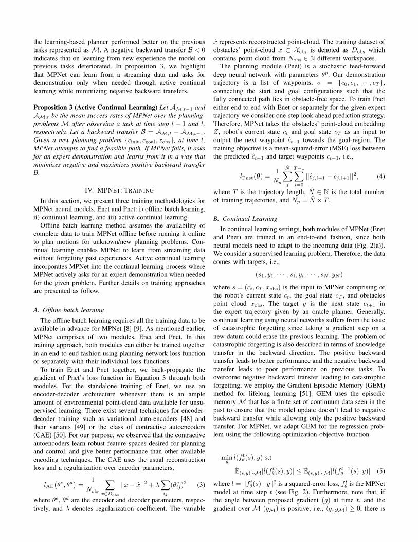
Fig. 4: Time comparison of MPNetPath with neural replanning (Red) and RRT* (Blue) for computing the near-optimal pathsolutions in example environments. Figs.(a-b) and (c-d) present simple 2D and complex 2D environments. Figs. (e-f) indicatescomplex 3D case whereas Figs. (g-h) shows the rigid-body case, also known as piano mover’s problem. In these environments,it can be seen that MPNet plans paths of comparable lengths as its expert demonstrator RRT* but in extremely shorter amountsof time.

Methods EnvironmentsSimple 2D Complex 2D Complex 3D Rigid-body

Informed-RRT* 1.06± 0.33 (1.10± 0.09) 1.60± 0.47 (1.49± 0.16) 2.99± 0.82 (2.76± 0.20) 15.58± 2.85 (14.80± 2.83)BIT* 0.59± 0.28 (0.65± 0.30) 1.79± 1.35 (1.61± 0.53) 0.19± 0.12 (0.20± 0.04) 7.16± 1.95 (6.52± 1.65)

MPNetSMP (B) 0.13± 0.01 (0.13± 0.00) 0.29± 0.05 (0.23± 0.07) 0.25± 0.05 (0.23± 0.06) 0.49± 0.05 (0.39± 0.04)MPNetPath:NP (C) 0.02± 0.00 (0.02± 0.00) 0.05± 0.01 (0.05± 0.01) 0.07± 0.01 (0.08± 0.01) 0.41± 0.08 (0.39± 0.07)

MPNetPath:NP (AC) 0.03± 0.01 (0.03± 0.01) 0.06± 0.01 (0.06± 0.01) 0.08± 0.01 (0.08± 0.01) 0.53± 0.12 (0.42± 0.08)MPNetPath:NP (B) 0.02± 0.00 (0.02± 0.00) 0.04± 0.00 (0.04± 0.01) 0.06± 0.01 (0.07± 0.01) 0.38± 0.04 (0.37± 0.02)MPNetPath:HP (B) 0.04± 0.03 (0.07± 0.04) 0.13± 0.07 (0.14± 0.09) 0.09± 0.03 (0.12± 0.04) 0.42± 0.30 (0.41± 0.40)

TABLE I: Mean computation times with standard deviations are presented for MPNet (all variations), Informed-RRT* and BIT*on two test datasets, i.e., seen and unseen (shown inside brackets), in four different environments. In all cases, MPNet pathplanners, MPnetPath:NP (with neural replanning) and MPnetPath:HP (with hybrid replanning), and sampler MPNetSMP withunderlying RRT*, trained with continual learning (C), active continual learning (AC) and offline batch learning (B), performedsignificantly better than classical planners such as Informed-RRT* and BIT* by an order of magnitude.

system used for training and testing has 3.40GHz× 8 IntelCore i7 processor with 32 GB RAM and GeForce GTX 1080GPU.

A. Training & Testing Environments

We consider problems requiring the planning of 2D/3Dpoint-mass robot, rigid-body, and a 7DOF Baxter robot manip-ulator. In case of 2D/3D point-mass and rigid-body planning,MPNet is trained over one hundred workspaces with eachcontaining four thousand trajectories, and it is evaluated ontwo test datasets, i.e., seen-Xobs and unseen-Xobs. The seen-Xobs comprises of one hundred workspaces seen by MPNetduring the training but two hundred unseen start and goal pairsin each environment. The unseen-Xobs consists of ten new

workspaces, not seen by MPNet during training, with eachcontaining two thousand start and goal pairs. For the 7DOFBaxter manipulator, we created a training dataset containingten cluttered environments with each having nine hundredtrajectories, and our test dataset contained the same tenworkspaces as in training but one hundred new start andgoal pairs for each scenario. For all planners, we evaluatemultiple trials on seen-Xobs and unseen-Xobs, and their meanperformance metrics are reported.

B. MPNet Comparison with its Expert Demonstrator (RRT*)

We compare MPNet against its expert demonstrator RRT*.Fig. 4 shows the paths generated by MPNetPath (red), and itsexpert demonstrator RRT* (blue). The average computations

(a) t = 0.13s, c = 32.46 (b) t = 0.13s, c = 38.02 (c) t = 0.25s, c = 27.57 (d) t = 0.21s, c = 37.23

(e) t = 0.22s, c = 40.73 (f) t = 0.18s, c = 36.48 (g) t = 0.29s, c = 39.51 (h) t = 0.21s, c = 40.26

Fig. 5: MPNetSMP generating informed samples for RRT* to plan motions in simple 2D (Figs. a-b), complex 2D (Figs c-d) andcomplex 3D (Figs. e-h). The number of samples and time required to compute the path are denoted by n and t, respectively. Ourexperiments show that MPNetSMP based RRT* is atleast 30 times faster than traditional RRT* in the presented environments.

0 20 40 60 80 100Environments

0

1

2

3

4

5

Tim

e (s

econ

ds)

Complex 3D


0

2

4

6

Tim

e (s

econ

ds)

Complex 2D


0

5

10

15

20

Tim

e (s

econ

ds)

Rigid Body


0.0

0.5

1.0

1.5

2.0

Tim

e (s

econ

ds)

Simple 2D

MPNetSMP (B) MPNetPath (AC) MPNetPath (B) IRRT* BIT* MPNetPath (C)

Fig. 6: Mean computation time comparisons of MPNetPath (with neural replanning) and MPNetSMP (with underlying RRT*)trained with offline batch learning (B), continual learning (C) and active continual learning (AC) against Informed-RRT* (IRR*)and BIT* on seen-Xobs dataset that comprises 100 environments and each environment contains 200 planning problems.

times of MPNetPath and RRT* are denoted as tR and tMP,respectively. The average Euclidean path cost of MPNetPathand RRT* solutions are denoted as cR and cMP, respectively.It can be seen that MPNet finds paths of similar lengths asits expert demonstrator RRT* while retaining consistently lowcomputational time. Furthermore, the computation times ofRRT* are not only higher than MPNetPath computation timebut also grows exponentially with the dimensionality of theplanning problems. Overall, we observed that MPNetPath isat least 100× faster than RRT* and finds paths that are withina 10% range of RRT*’s paths cost.

Fig. 5 presents informed trees generated by MPNetSMPwith an underlying RRT* algorithm. We report average pathcomputation times and Euclidean costs denoted as t and c,respectively. The generated trees by MPNetSMP are in a

subspace of given configuration space that most of the timecontains path solutions. It should be noted that MPNetSMPpaths are almost optimal and are observed to be better thanMPNetPath and its expert demonstrator RRT* solutions. More-over, our sampler not only finds near-optimal/optimal pathsbut also exhibit a consistent computation time of less thana second in all environments which is much lower than thecomputation time of RRT* algorithm. Thus, MPNetSMP haseffectively made the underlying SMP (in this case, RRT*) amore efficient motion planner.

C. MPNet Comparison with Advanced Motion Planners

We further extend our comparative studies to evaluateMPNet against advanced classical planners such as Informed-RRT* [2] and BIT* [3].

0 2 4 6 8Environments

0.0

0.5

1.0

1.5

2.0

2.5

3.0

Tim

e (s

econ

ds)

Complex 3D


0.0

0.1

0.2

0.3

0.4

0.5

Tim

e (s

econ

ds)

Complex 2D


0

5

10

15

20

Tim

e (s

econ

ds)

Rigid Body


0.0

0.2

0.4

0.6

0.8

1.0

1.2

1.4

Tim

e (s

econ

ds)

Simple 2D

MPNetSMP (B) MPNetPath (AC) MPNetPath (B) IRRT* BIT* MPNetPath (C)

Fig. 7: Mean computation time comparisons of MPNetPath (with neural replanning) and MPNetSMP (with underlying RRT*)against Informed-RRT* (IRRT*) and BIT* on unseen-Xobs dataset that comprises unseen 10 environments and each environmentcontains 2000 planning problems. The training methods for MPNet includes offline batch learning (B), continual learning (C)and active continual learning (AC).

Methods EnvironmentsSimple 2D Complex 2D Complex 3D Rigid-body

MPNetPath:NP (C) 93.33 (93.18) 83.44 (83.78) 89.88 (90.86) 83.770 (86.18)MPNetPath:NP (AC) 96.70 (97.83) 84.36 (84.08) 96.60 (95.28) 87.08 (87.64)MPNetPath:NP (B) 99.30 (98.30) 99.71 (98.80) 99.11 (97.76) 94.21 (95.18)MPNetPath:HP (B) 100.0 (100.0) 100.0 (100.0) 100.0 (100.0) 100.0 (100.0)

MPNetSMP 100.0 (100.0) 100.0 (100.0) 100.0 (100.0) 100.0 (100.0)

TABLE II: Success rates of all MPNet variants in the four environments on both test datasets, seen and unseen (shown insidebrackets).

simple 2D complex 2D complex 3D rigid-body0

50

100

150

200

250

300

350

400

no. o

f tra

inin

g pa

ths (

x100

0)

Active Continual LearningBatch/Continual Learning

Fig. 8: The number of training trajectories required by MPNetwhen trained with active continual learning as compared totraditional batch/ continual learning approaches. It can be seenthat active continual training exhibits significant improvementin data-efficiency and yet provides similar performance asconventional methods (Table I & II).

Table I presents the comparison results over the four dif-ferent scenarios, i.e., simple 2D (Fig. 4 (a-b)), complex 2D(Fig. 4 (c-d)), complex 3D (Fig. 4 (e-f)) and rigid-body (Fig.4 (g-h)). Each scenario comprises of two test datasets, seen-Xobs and unseen-Xobs. We let Informed-RRT* and BIT* rununtil they find a solution of Euclidean cost within 5% range ofthe cost of MPNetPath solution. We report mean computationtimes with standard deviation over five trials. In all planningproblems, MPNetPath:NP (with neural replanning), MPNet-

Path:HP (with hybrid replanning), and MPNetSMP exhibit amean computation time of less than a second. The state-of-the-art classical planners, Informed-RRT* and BIT*, not onlyexhibit higher computation times than all versions of MPNetbut, just-like RRT*, their computation times increase with theplanning problem dimensionality. In simplest case (Fig. 4 (a-b)), MPNetPath:NP stand out to be atleast 80× and 30× fasterthan BIT* and Informed-RRT*, respectively. On the otherhand, MPNetSMP provides about 8× and 5× computationspeed improvements compared to BIT* and Informed-RRT*,respectively, in simple 2D environments. Furthermore, it canbe observed that the speed gap between classical planner andMPNet (MPNetPath and MPNetSMP) keeps increasing withplanning problem dimensions.

Fig. 6 and Fig. 7 present the mean computation time of allMPNet variants, Informed-RRT* (IRRT*), and BIT* on seen-Xobs and unseen-Xobs test datasets, respectively. Note thatMPNetPath trained with offline batch learning (B), continuallearning (C), and active continual learning (AC) show similarcomputation times as can be seen by their plots hugging eachother in all planning problems. Furthermore, in Figs. 6-7, itcan be seen that MPNetPath and MPNetSMP computationtimes remain consistently less than one second in all planningproblems irrespective of their dimensions. The computationtimes of IRRT* and BIT* are not only high but also lack con-sistency and exhibits high variations over different planningproblems. Although the computation speed of MPNetSMP isslightly lower than that of MPNetPath, it performs better thanall other methods in terms of path optimality for a given costfunction.

Envi

ronm

ent 4

Envi

ronm

ent 3

Envi

ronm

ent 2

Envi

ronm

ent 1

Goal configurationStart configuration Intermediate configurations

Fig. 9: We evaluated MPNetPath (with neural replanning) to plan motion for a Baxter robot in ten challenging and clutteredenvironments, out of which four are shown in this figure. The figures on the left-most and right-most indicate the robot atinitial and goal configurations, respectively, whereas the blue duck shows the target positions. In these scenarios, MPNet tookless than a second whereas BIT* took about 9 seconds to find solutions. In these settings, we observed that BIT* solutionshas almost 40% higher path lengths than MPNet solutions.

D. MPNet Data Efficiency & Performance Evaluation

Fig. 8 shows the number of training paths consumed byall MPNet versions and Table II presents their mean suc-cess rates on the test datasets in four scenarios- simple 2D,complex 2D, complex 3D, and rigid-body. The success raterepresents the percentage of planning problems solved bya planner in a given test dataset. The models trained withoffline batch learning provides better performance in term ofa success rate compared to continual/active-continual learningmethods. However, in our experiments, the continual/active-continual learning frameworks required about ten trainingepochs compared to one hundred training epochs of theoffline batch learning method. Furthermore, we observed thatcontinual/active-continual learning and offline batch learningshow similar success rates if allowed to run for the samenumber of training epochs. The active continual learning isultimately preferred as it requires less training data thantraditional continual and offline batch learning while exhibitingconsiderable performance.

E. MPNet on 7DOF Baxter

Since BIT* performs better than Informed-RRT* in highdimension planning problems, we consider only BIT* asour classical planner in our further comparative analysis.We evaluate MPNet against BIT* for the motion planningof 7DOF Baxter robot in ten different environments whereeach environment comprised of one hundred new planningproblems. Fig. 9 presents four out of ten environment settings.Each planning problem scenario contained an L-shape table ofhalf the Baxter height with randomly placed five different real-world objects such as a book, bottle, or mug as shown in thefigure. The planner’s objective is to find a path from a givenrobot configuration to target configuration while avoiding anycollisions with the environment, or self-collisions. Table IIIsummarizes the results over the entire test dataset. MPNeton average find paths in less than a second with about 80%success rate. BIT* also finds the initial path in less than asecond with similar success rate as MPNet. However, the pathcosts of BIT* initial solution are significantly higher than thepath cost of MPNet solutions. Furthermore, we let BIT* run toimprove its initial path solutions so that the cost of the paths

1 2 3 4

5 6 7 8

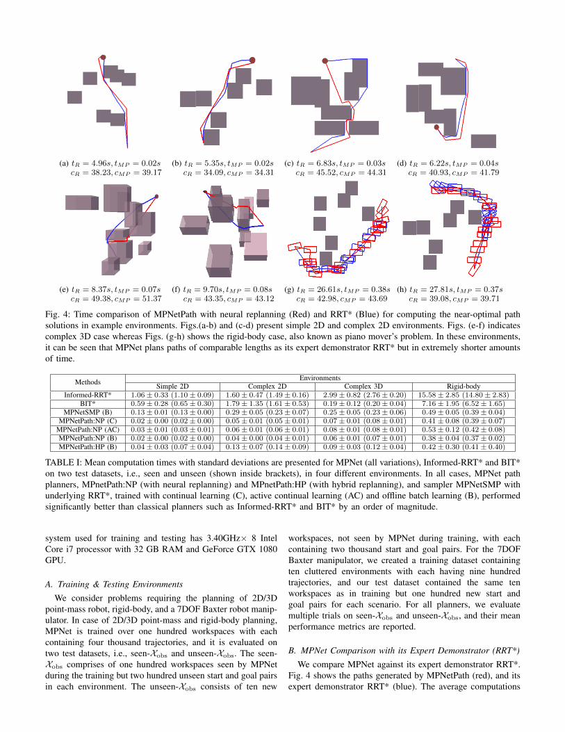
Fig. 10: MPNetPath plans motion for a multi-target problem. The task is to pick up the blue object (duck), by planning a pathfrom the initial robot position (Frame 1) to graspable object location (Frame 5), and move it to a new target (yellow block)(Frame 8). Note that the stopwatch indicates the execution time not the planning time. Furthermore, MPNet was never trainedon any path connecting any two positions on the table-top, yet MPNet successfully planned the motion which indicates itsability to generalize to new planning problems. In this scenario, MPNetPath (with neural replanning) computed the entire pathplan in subsecond whereas BIT* took about few minutes to find a solution that is within 10% cost of MPNet path solution.

Methods BaxterTime Path cost Success rate(%)

BIT* (Initial Path) 0.94± 0.20 13.91± 0.60 83.0BIT* (±40% MPNet cost) 9.20± 7.61 10.78± 0.31 56.0

MPNetPath (C) 0.81± 0.08 6.98± 0.18 78.6MPNetPath (B) 0.59± 0.08 7.86± 0.20 87.8

TABLE III: Computation time, path cost/length, and success rate comparison of MPNetPath (with neural replanning) trainedwith offline batch (B) and continual (C) learning against BIT* on Baxter test dataset. In case of BIT*, the times for findingthe first path and further optimizing it to a path cost within 40% range of MPNet’s path cost are reported. Overall, MPNetexhibits superior performance than BIT* in terms of path costs, mean computation times, and success rates.

are not greater than 140% of MPNet path costs. The resultsshow that BIT* mostly fails to find solutions as optimal asMPNet solutions but demonstrate about 56% success rate infinding solutions that are usually 40% larger in lengths/coststhan MPNet path costs. Furthermore, the computation timeof BIT* also increases significantly, requiring an average ofabout 9 seconds to plan such paths. Fig. 11 shows the meancomputation time and path cost comparison of BIT* andMPNet over ten individual environments. It can be seen thatMPNet computes paths in less than a second while givingincredibly optimized solutions and is much faster comparedto BIT*.

Fig. 10 shows a multi-goal planning problem for 7 DOFBaxter robot. The task is to reach and pick up the target objectwhile avoiding any collision with the environment and transferit to another target location, shown as yellow block. Note thatin previous experiments we let BIT* run until it finds pathswithin 40% of MPNet path costs. Now, we let BIT* run untilit finds a path within 10% cost of the cost of MPNet pathsolution. Our result shows that MPNetPath:NP plans the entiretrajectory in less than a second whereas BIT* took about 3.01minutes to find a path of similar cost as our solution. Notethat MPNet is never trained on trajectories that connect twoconfigurations on the table. However, thanks to MPNet abilityto generalize that it can solve completely unseen problems inno time compared to classical planners that have to performan exhaustive search before proposing any path solution.

VII. DISCUSSION

This section presents a discussion on various attributes ofMPNet, sample selection methods for continual learning, anda brief analysis of its completeness, optimality, and computa-tional guarantees.

A. Stochastic Neural Planner

In MPNet, we apply Dropout [54] to almost every layerof the planning network, and it remains active during pathplanning. The Dropout randomly selects the neurons from itspreceding layer with a probability p ∈ [0, 1] and masks themso that they do not affect the model decisions. Therefore, atany planning step, Pnet would have a probabilistically differentmodel structure that results in stochastic behavior.

Yarin and Zubin [59] demonstrate the application ofDropout to model uncertainty in the neural networks. We showthat the Dropout can also be used in learning-based motionplanners to approximate the subspace of a given configurationspace that potentially contains several path solutions to a givenplanning problem. For instance, it is evident from the treesgenerated by MPNetSMP (Fig. 5) that our model approximatesthe subspace containing path solutions including the optimalpath.

The perturbations in Pnet’s output, thanks to Dropout, alsoplay a crucial role during our neural replanning (Algorithm4). In neural replanning, MPNet takes its own global path anduses its stochastic neural planner (Algorithm 5) to replan amotion between any beacon states in that global path. MPNet


0

5

10

15

20

Tim

e (s

econ

ds)

Average Planning Times For BaxterMPNetPath (B)MPNetPath (C)BIT* (initial path)BIT* (Within 40% MPNet cost)


7

8

9

10

11

12

13

14

15

Path

cos

t

Average Path Costs For BaxterMPNetPath (B)MPNetPath (C)BIT* (initial path)BIT* (Within 40% MPNet cost)

Fig. 11: Computational time and path length comparison ofMPNet (trained using batch (B) and continual (C) training)against BIT* over ten challenging environments that requiredpath planning of a 7DOF Baxter. BIT* exhibits similar com-putation time for finding initial paths as MPNet, but the pathlengths of BIT* solutions are significantly larger than pathlengths of MPNet solutions.

is able to recover from any failures or anomalies that hinderedfinding a feasible solution in the first place.

B. Sample Selection Strategies

In continual learning, we maintain an episodic memory of asubset of past training data to mitigate catastrophic forgettingwhen training MPNet on new demonstrations. Therefore, itis crucial to populate the episodic memory with examplesthat are important for learning a generalizable model fromstreaming data. We compare four MPNet models trained ona simple 2D environment with four different sample selectionstrategies for the episodic memory. The four selection metricsinclude surprise, reward, coverage maximization, and globaldistribution matching. The surprise and reward metrics givehigher and lower priority to examples with large predictionerrors, respectively. The coverage maximization maintains a

memory of k-nearest neighbors. The global distribution match-ing, as described earlier, uses random selection techniquesto approximate the global distribution from streaming data.We evaluate four MPNet models on two test datasets, seen-Xobs and unseen-Xobs, from simple 2D environment, andtheir mean success rates are reported in Fig. 12. It can beseen that global distribution matching exhibits slightly betterperformance than reward and coverage maximization metrics.The surprise metric gives poor performance because satisfyingthe constraint in Equations 7 becomes nearly impossible whenthe episodic memory is populated with examples that havelarge prediction losses. Since global distribution matchingprovides the best performance overall, we have used it asour sample selection strategy for the episodic memory in thecontinual learning settings.

0 50 100 150 200 250 300 350 400Evaluation iterations

65

70

75

80

85

90

95

Succ

ess r

ate

(%)

Performance on seen test environments

Distribution matchingSurpriseRewardCoverage maximization

0 50 100 150 200 250 300 350 400Evaluation iterations

70

75

80

85

90

95

Succ

ess r

ate

(%)

Performance on unseen test environments

Distribution matchingSurpriseRewardCoverage maximization

Fig. 12: Impact of sample selection methods for episodememory on the performance of continual learning for MPNetin simple 2D test datasets seen-Xobs and unseen-Xobs.

C. Completeness

In this section, we discuss the completeness guarantees(Proposition 1) of MPNet (MPNetPath and MPNetSMP)which imply that for a given planning problem, MPNet will

eventually find a feasible path, if one exists. We show that theworst-case completeness guarantees of our approach rely onthe underlying SMP for both path planning (MPNetPath) andinformed neural sampling (MPNetSMP). In our experiments,we use RRT* as our oracle SMP. RRT* exhibits probabilisticcompleteness.

The probabilistic completeness is described in Definition 1based on the following notations. Let T ALn be a connectedtree in obstacle-free space, comprising of n vertices, generatedby an algorithm AL. We also assume T ALn always originatesfrom the robot’s initial configuration cinit. An algorithmis probabilistically complete if it satisfies the followingdefinition.

Definition 1 (Probabilistic Completeness) Given aplanning problem {cinit, cgoal,Xobs} for which thereexists a solution, an algorithm AL with a tree T ALn thatoriginates at cinit is considered probabilistically complete ifflimn→∞ P(T ALn ∩ cgoal 6= ∅) = 1.

RRT* algorithm exhibits probabilistic completeness as itbuilds a connected tree originating from initial robot config-uration and randomly exploring the entire space until it findsa goal configuration. Therefore, as the number of samples inthe RRT* approach to infinity the probability of finding a pathsolution, if one exists, gets to one, i.e.,

limn→∞

P(T RRT∗

n ∩ cgoal 6= ∅) = 1 (8)

In remainder of the section, we present a brief analysisshowing that MPNetPath and MPNetSMP also exhibitprobabilistic completeness like their underlying RRT*.

1) Probabilistic completeness of MPNetPath: To justifyMPNetPath worst-case guarantees, we introduce the followingassumptions that are crucial to validate a planning problem.

Assumption 1 (Feasibility of States to Connect) Thegiven start and goal pairs (cinit, cgoal), for which an oracle-planner is called to find a path, lie entirely in obstacle-freespace, i.e., cinit ∈ Cfree and cgoal ⊂ Cfree.

Assumption 2 (Existence of a Path Solution) UnderAssumption 1, for a given problem (cinit, cgoal,Xobs), thereexists at least one feasible path σ that connects cinit andcgoal, and σ 6⊂ Xobs.

Based on Definition 1 and Assumptions 1-2, we propose inTheorem 1, with a sketch of proof, that MPNetPath alsoexhibits probabilistic completeness, just like its underlyingoracle planner RRT*.

Theorem 1 (Probabilistic Completeness of MPNetPath)If Assumptions 1-2 hold, for a given planning problem{cinit, cgoal,Xobs}, and an oracle RRT* planner, MPNetPathwill find a path solution, if one exists, with a probability of oneas the underlying RRT* is allowed to run till infinity if needed.

Sketch of Proof: Assumption 1 puts a condition that

the start and goal states in the given planning problemlie in the obstacle-free space. Assumption 2 requires thatthere exist at least one collision-free trajectory for the givenplanning problem. During planning, MPNetPath first finds acoarse solution σ that might have beacon (non-connectableconsecutive) states (see Fig. 3). Our algorithm connects thosebeacon states through replanning. Assumption 1 holds forthe beacon states as each generated state of MPNetPath isevaluated by an oracle collision-checker before making it apart of σ. In replanning, we perform neural replanning fora fixed number of trials to further refine σ, and if that failsto conclude a solution, we connect any remaining beaconstates of the refined σ by RRT*. Hence, if Assumption 1-2hold for beacon states, MPNetPath inherits the convergenceguarantees of the underlying planner which in our case isRRT*. Therefore, MPNetPath with an underlying RRT*oracle planner exhibits probabilistic completeness.

2) Probabilistic completeness of MPNetSMP: MPNetSMPgenerates samples for SMPs such as RRT*. Our methodperforms exploitation and exploration to build an informedtree. It begins with exploitation by sampling a subspacethat potentially contains a solution for a limited time andswitches to exploration via uniform sampling to cover theentire configuration space. Therefore, like RRT*, the tree ofMPNetSMP is fully connected, originates from the initial robotconfiguration, and eventually expands to explore the entirespace. Hence, the probability that MPNetSMP tree will find agoal configuration, if possible, approaches one as the samplesin the tree reaches a large number, i.e.,

limn→∞

P(T MPNetSMPn ∩ cgoal 6= ∅) = 1 (9)

D. Optimality

MPNet learns through imitating the expert demonstrationswhich could come from either an oracle motion planner ora human demonstrator. In our experiments, we use RRT* forgenerating expert trajectories, hybrid replanning in MPNet-Path, and as a baseline SMP for our MPNetSMP framework.We show that MPNetPath imitates the optimality of its expertdemonstrator. In Fig. 5, it can be seen that MPNet path solu-tions are of similar Euclidean costs as its expert demonstratorRRT* path solutions. Therefore, the quality of the MPNetpaths relies on the quality of its training data.

In the case of MPNetSMP, there exists optimality guaran-tees depending on the underlying SMP. Since we use RRT*as a baseline SMP for MPNetSMP, the proposed methodexhibits asymptotic optimality. Asymptotically optimal SMP,like RRT*, eventually converge to a minimum cost pathsolution, if one exists, as the number of samples in the treeapproaches to infinity (for proof, refer to [1]). RRT* getsweak-optimality guarantees from its rewiring heuristic. Therewiring incrementally updates the tree connections such thatover the time, each node in the tree would be connected to abranch that ensures lowest cost path to the root state (initialrobot configuration) of the tree. Therefore, due to rewiring,RRT* asymptotically guarantees the shortest path between thegiven start and goal states.

In our sampling heuristic, MPNetSMP generates informedsamples for a fixed number of iterations and performs uniformrandom sampling afterward. Therefore, RRT* tree formed bythe samples of MPNetSMP will explore the entire C-space andwill be rewired incrementally to ensure asymptotic optimality.Since MPNetSMP only performs intelligent sampling and doesnot modify the internal machinery of RRT*, the optimalityproofs will exactly be the same as provided in [1].

E. Computational Complexity

In this section, we present the computational complexity ofour method. Both MPnetPath and MPNetSMP take the outputof Enet and Pnet, which is only a forward-pass through aneural network. The forward pass through a neural networkis known to have a constant complexity since it is a matrixmultiplication of a fixed size input vector with network weightsto generate a fixed size output vector. Since MPNetSMP pro-duces samples by merely forward passing a planning problemthrough Enet and Pnet, it does not add any complexity tothe underlying SMP. Therefore, the computational complexityof MPNetSMP with underlying RRT* is the same as RRT*complexity, i.e., O(n log n), where n is the number of samples[1].

On the other hand, MPNetPath has a crucial replanningcomponent that uses an oracle planner in the cases whereneural replanning fails to determine an end-to-end collision-free path. The oracle planner in the presented experimentsis RRT*. Therefore, in the worst-case, MPNetPath operateswith complexity of O(n log n). However, we show empiricallythat MPNetPath succeeds, without any oracle planner, forup to 90% of the cases in a challenging test dataset. Forthe remaining 10% cases, oracle planner is executed onlyfor a small segment of the overall path (see Algorithm 5).Hence, even for hard planning problems where MPNetPathfails, our method reduces a complicated problem into a simplerproblem, thanks to its divide-and-conquer approach, for theunderlying oracle planner. Thus, the oracle planner operates ata complexity which is practically much lower than its worst-case theoretical complexity, as is also evident from the resultsof MPNetPath with hybrid replanning (HB) in Table I.

VIII. CONCLUSIONS AND FUTURE WORK

We present a learning-based approach to motion planningusing deep neural networks. For a given planning problem,our method is capable of i) finding collision-free near-optimalpaths; ii) generating samples for sampling-based motion plan-ners in a subspace of a given configuration space that mostlikely contains solutions including the optimal path. We alsopresent the active continual learning strategy to train our mod-els with a significant improvement in training data-efficiencycompared to naive training approaches. Our experimenta-tion shows that our neural motion planner consistently findscollision-free paths in less than a second for the problemswhere other planners may take up to several minutes.

In our future works, one of our primary objectives is totackle the environment encoding problem for motion planning.Environment encoding is one of the critical challenges in

real-world robotics problems. Current perception approachesconsider encoding of individual objects rather than the entirescene that retains the inter-object relational geometry which iscrucial for motion planning. Henceforth, we aim to address theproblem of motion planning oriented environments’ encodingfrom raw point-cloud data. Another future objective is to learnall fundamental modules required for motion planning thatnot only include the motion planner but also the collisionchecker and cost function. Recently, L2RRT [47] is proposedthat learns the motion planner and collision checker in latentspace. However, providing worst-case theoretical guaranteesis notoriously hard for planning in latent spaces. Therefore,a modular approach is necessary that learns decision-makingdirectly in robot configuration space so that it can be combinedwith any classical motion planner to provide theoretical guar-antees. Furthermore, learning a cost function, using inversereinforcement learning [60], is also crucial for kinodynamicand constraint motion planning problems where defining a costfunction satisfying all constraints is challenging.

REFERENCES

[1] S. Karaman and E. Frazzoli, “Sampling-based algorithms for optimalmotion planning,” The international journal of robotics research, vol. 30,no. 7, pp. 846–894, 2011.

[2] J. D. Gammell, S. S. Srinivasa, and T. D. Barfoot, “Informed rrt*:Optimal sampling-based path planning focused via direct sampling of anadmissible ellipsoidal heuristic,” in Intelligent Robots and Systems (IROS2014), 2014 IEEE/RSJ International Conference on. IEEE, 2014, pp.2997–3004.

[3] J. D. Gammell, S. Srinivasa, and T. D. Barfoot, “Batch informed trees(bit*): Sampling-based optimal planning via the heuristically guidedsearch of implicit random geometric graphs,” in Robotics and Automa-tion (ICRA), 2015 IEEE International Conference on. IEEE, 2015, pp.3067–3074.

[4] S. M. LaValle, Planning algorithms. Cambridge university press, 2006.[5] J.-C. Latombe, Robot motion planning. Springer Science & Business

Media, 2012, vol. 124.[6] O. Khatib, “Real-time obstacle avoidance for manipulators and mobile

robots,” in Autonomous robot vehicles. Springer, 1986, pp. 396–404.[7] N. Haghtalab, S. Mackenzie, A. D. Procaccia, O. Salzman, and S. S.

Srinivasa, “The provable virtue of laziness in motion planning,” inTwenty-Eighth International Conference on Automated Planning andScheduling, 2018.

[8] A. H. Qureshi, A. Simeonov, M. J. Bency, and M. C. Yip, “Motionplanning networks,” arXiv preprint arXiv:1806.05767, 2019.

[9] A. H. Qureshi and M. C. Yip, “Deeply informed neural sampling forrobot motion planning,” in 2018 IEEE/RSJ International Conference onIntelligent Robots and Systems (IROS). IEEE, 2018, pp. 6582–6588.

[10] J. T. Schwartz and M. Sharir, “On the piano movers problem. ii.general techniques for computing topological properties of real algebraicmanifolds,” Advances in applied Mathematics, vol. 4, no. 3, pp. 298–351, 1983.

[11] T. Lozano-Perez and M. A. Wesley, “An algorithm for planning collision-free paths among polyhedral obstacles,” Communications of the ACM,vol. 22, no. 10, pp. 560–570, 1979.

[12] J. Canny, The complexity of robot motion planning. MIT press, 1988.[13] R. A. Brooks and T. Lozano-Perez, “A subdivision algorithm in config-

uration space for findpath with rotation,” IEEE Transactions on Systems,Man, and Cybernetics, no. 2, pp. 224–233, 1985.

[14] S. M. LaValle, “Rapidly-exploring random trees: A new tool for pathplanning,” 1998.

[15] L. E. Kavraki and J.-C. Latombe, “Probabilistic roadmaps for robot pathplanning,” 1998.

[16] K. Hauser, “Lazy collision checking in asymptotically-optimal motionplanning,” in 2015 IEEE International Conference on Robotics andAutomation (ICRA). IEEE, 2015, pp. 2951–2957.

[17] A. H. Qureshi and Y. Ayaz, “Potential functions based sampling heuristicfor optimal path planning,” Autonomous Robots, vol. 40, no. 6, pp. 1079–1093, 2016.

[18] A. H. Qureshi, S. Mumtaz, K. F. Iqbal, B. Ali, Y. Ayaz, F. Ahmed,M. S. Muhammad, O. Hasan, W. Y. Kim, and M. Ra, “Adaptivepotential guided directional-rrt,” in 2013 IEEE International Conferenceon Robotics and Biomimetics (ROBIO). IEEE, 2013, pp. 1887–1892.

[19] A. H. Qureshi and Y. Ayaz, “Intelligent bidirectional rapidly-exploringrandom trees for optimal motion planning in complex cluttered environ-ments,” Robotics and Autonomous Systems, vol. 68, pp. 1–11, 2015.

[20] Z. Tahir, A. H. Qureshi, Y. Ayaz, and R. Nawaz, “Potentially guidedbidirectionalized rrt* for fast optimal path planning in cluttered environ-ments,” Robotics and Autonomous Systems, vol. 108, pp. 13–27, 2018.

[21] B. Hou and S. Srinivasa, “Deep conditional generative models forheuristic search on graphs with expensive-to-evaluate edges.”

[22] R. S. Sutton, A. G. Barto et al., Introduction to reinforcement learning.MIT press Cambridge, 1998, vol. 135.

[23] T. P. Lillicrap, J. J. Hunt, A. Pritzel, N. Heess, T. Erez, Y. Tassa,D. Silver, and D. Wierstra, “Continuous control with deep reinforcementlearning,” arXiv preprint arXiv:1509.02971, 2015.

[24] M. P. Deisenroth, G. Neumann, J. Peters et al., “A survey on policysearch for robotics,” Foundations and Trends R© in Robotics, vol. 2, no.1–2, pp. 1–142, 2013.

[25] J. Kober, J. A. Bagnell, and J. Peters, “Reinforcement learning inrobotics: A survey,” The International Journal of Robotics Research,vol. 32, no. 11, pp. 1238–1274, 2013.

[26] V. Mnih, K. Kavukcuoglu, D. Silver, A. A. Rusu, J. Veness, M. G.Bellemare, A. Graves, M. Riedmiller, A. K. Fidjeland, G. Ostrovskiet al., “Human-level control through deep reinforcement learning,”Nature, vol. 518, no. 7540, p. 529, 2015.

[27] Y. Duan, X. Chen, R. Houthooft, J. Schulman, and P. Abbeel, “Bench-marking deep reinforcement learning for continuous control,” in Inter-national Conference on Machine Learning, 2016, pp. 1329–1338.

[28] S. Levine, C. Finn, T. Darrell, and P. Abbeel, “End-to-end training ofdeep visuomotor policies,” The Journal of Machine Learning Research,vol. 17, no. 1, pp. 1334–1373, 2016.

[29] S. Levine, P. Pastor, A. Krizhevsky, J. Ibarz, and D. Quillen, “Learninghand-eye coordination for robotic grasping with deep learning and large-scale data collection,” The International Journal of Robotics Research,vol. 37, no. 4-5, pp. 421–436, 2018.

[30] A. Yahya, A. Li, M. Kalakrishnan, Y. Chebotar, and S. Levine,“Collective robot reinforcement learning with distributed asynchronousguided policy search,” in 2017 IEEE/RSJ International Conference onIntelligent Robots and Systems (IROS). IEEE, 2017, pp. 79–86.

[31] Y. Chebotar, M. Kalakrishnan, A. Yahya, A. Li, S. Schaal, and S. Levine,“Path integral guided policy search,” in 2017 IEEE international confer-ence on robotics and automation (ICRA). IEEE, 2017, pp. 3381–3388.

[32] S. Gu, E. Holly, T. Lillicrap, and S. Levine, “Deep reinforcementlearning for robotic manipulation with asynchronous off-policy updates,”in 2017 IEEE international conference on robotics and automation(ICRA). IEEE, 2017, pp. 3389–3396.

[33] I. Popov, N. Heess, T. Lillicrap, R. Hafner, G. Barth-Maron, M. Ve-cerik, T. Lampe, Y. Tassa, T. Erez, and M. Riedmiller, “Data-efficientdeep reinforcement learning for dexterous manipulation,” arXiv preprintarXiv:1704.03073, 2017.

[34] A. H. Qureshi, J. J. Johnson, Y. Qin, B. Boots, and M. C. Yip,“Composing ensembles of policies with deep reinforcement learning,”arXiv preprint arXiv:1905.10681, 2019.

[35] M. Zucker, J. Kuffner, and J. A. Bagnell, “Adaptive workspace biasingfor sampling-based planners,” in Robotics and Automation, 2008. ICRA2008. IEEE International Conference on. IEEE, 2008, pp. 3757–3762.

[36] R. J. Williams, “Simple statistical gradient-following algorithms forconnectionist reinforcement learning,” Machine learning, vol. 8, no. 3-4,pp. 229–256, 1992.

[37] D. Berenson, P. Abbeel, and K. Goldberg, “A robot path planningframework that learns from experience,” in Robotics and Automation(ICRA), 2012 IEEE International Conference on. IEEE, 2012, pp.3671–3678.

[38] D. Coleman, I. A. Sucan, M. Moll, K. Okada, and N. Correll,“Experience-based planning with sparse roadmap spanners,” in Roboticsand Automation (ICRA), 2015 IEEE International Conference on. IEEE,2015, pp. 900–905.

[39] G. Ye and R. Alterovitz, “guided motion planning,” in Robotics research.Springer, 2017, pp. 291–307.

[40] M. J. Bency, A. H. Qureshi, and M. C. Yip, “Neural path planning: Fixedtime, near-optimal path generation via oracle imitation,” arXiv preprintarXiv:1904.11102, 2019.

[41] B. Ichter, J. Harrison, and M. Pavone, “Learning sampling distributionsfor robot motion planning,” in 2018 IEEE International Conference onRobotics and Automation (ICRA). IEEE, 2018, pp. 7087–7094.

[42] L. Janson and M. Pavone, “Fast marching trees: A fast marchingsampling-based method for optimal motion planning in many dimen-sions,” in Robotics Research. Springer, 2016, pp. 667–684.

[43] C. Zhang, J. Huh, and D. D. Lee, “Learning implicit sampling distribu-tions for motion planning,” in 2018 IEEE/RSJ International Conferenceon Intelligent Robots and Systems (IROS). IEEE, 2018, pp. 3654–3661.

[44] M. Bhardwaj, S. Choudhury, and S. Scherer, “Learning heuristic searchvia imitation,” arXiv preprint arXiv:1707.03034, 2017.

[45] A. Tamar, Y. Wu, G. Thomas, S. Levine, and P. Abbeel, “Value iterationnetworks,” in Advances in Neural Information Processing Systems, 2016,pp. 2154–2162.

[46] A. Srinivas, A. Jabri, P. Abbeel, S. Levine, and C. Finn, “Universalplanning networks,” arXiv preprint arXiv:1804.00645, 2018.

[47] B. Ichter and M. Pavone, “Robot motion planning in learned latentspaces,” IEEE Robotics and Automation Letters, 2019.

[48] D. P. Kingma and M. Welling, “Auto-encoding variational bayes,” arXivpreprint arXiv:1312.6114, 2013.

[49] I. Higgins, L. Matthey, A. Pal, C. Burgess, X. Glorot, M. Botvinick,S. Mohamed, and A. Lerchner, “beta-vae: Learning basic visual conceptswith a constrained variational framework,” in International Conferenceon Learning Representations, vol. 3, 2017.

[50] S. Rifai, P. Vincent, X. Muller, X. Glorot, and Y. Bengio, “Contractiveauto-encoders: Explicit invariance during feature extraction,” in Proceed-ings of the 28th International Conference on International Conferenceon Machine Learning. Omnipress, 2011, pp. 833–840.

[51] D. Lopez-Paz et al., “Gradient episodic memory for continual learning,”in Advances in Neural Information Processing Systems, 2017, pp. 6467–6476.

[52] D. Isele and A. Cosgun, “Selective experience replay for lifelonglearning,” in Thirty-Second AAAI Conference on Artificial Intelligence,2018.

[53] D. Rolnick, A. Ahuja, J. Schwarz, T. P. Lillicrap, and G. Wayne, “Expe-rience replay for continual learning,” arXiv preprint arXiv:1811.11682,2018.

[54] N. Srivastava, G. E. Hinton, A. Krizhevsky, I. Sutskever, andR. Salakhutdinov, “Dropout: a simple way to prevent neural networksfrom overfitting.” Journal of machine learning research, vol. 15, no. 1,pp. 1929–1958, 2014.

[55] J. J. Kuffner Jr and S. M. LaValle, “Rrt-connect: An efficient approachto single-query path planning,” in ICRA, vol. 2, 2000.

[56] K. Hauser and V. Ng-Thow-Hing, “Fast smoothing of manipulatortrajectories using optimal bounded-acceleration shortcuts,” in 2010 IEEEinternational conference on robotics and automation. IEEE, 2010, pp.2493–2498.

[57] S. Skiena, “Implementing discrete mathematics: combinatorics andgraph theory with mathematica1991.”

[58] I. A. Sucan, M. Moll, and L. E. Kavraki, “The Open Motion PlanningLibrary,” IEEE Robotics & Automation Magazine, vol. 19, no. 4, pp.72–82, December 2012, http://ompl.kavrakilab.org.

[59] Y. Gal and Z. Ghahramani, “Dropout as a bayesian approximation:Representing model uncertainty in deep learning,” in internationalconference on machine learning, 2016, pp. 1050–1059.

[60] A. H. Qureshi, B. Boots, and M. C. Yip, “Adversarial imitationvia variational inverse reinforcement learning,” in InternationalConference on Learning Representations, 2019. [Online]. Available:https://openreview.net/forum?id=HJlmHoR5tQ

[61] L. Trottier, P. Giguere, and B. Chaib-draa, “Parametric exponentiallinear unit for deep convolutional neural networks,” arXiv preprintarXiv:1605.09332, 2016.

[62] J. Duchi, E. Hazan, and Y. Singer, “Adaptive subgradient methodsfor online learning and stochastic optimization,” Journal of MachineLearning Research, vol. 12, no. Jul, pp. 2121–2159, 2011.

[63] R. B. Rusu and S. Cousins, “Point cloud library (pcl),” in 2011 IEEEinternational conference on robotics and automation, 2011, pp. 1–4.

http://ompl.kavrakilab.org

https://openreview.net/forum?id=HJlmHoR5tQ

Environment Training Mode Model ArchitectureSimple 2D B/C/AC 32→ 1280→ 1024→ 896→ 768→ 512→ 384→ 256→ 256→ 128→ 64→ 32→ 2

Complex 2D B 32→ 1280→ 1024→ 896→ 768→ 512→ 384→ 256→ 256→ 128→ 64→ 32→ 2C/AC 32→ 1024→ 768→ 512→ 512→ 128→ 64→ 2

Complex 3D B/C/AC 66→ 1280→ 1024→ 896→ 768→ 512→ 384→ 256→ 256→ 128→ 64→ 32→ 3

RigidB 34→ 1280→ 1024→ 896→ 768→ 512→ 384→ 256→ 256→ 128→ 64→ 32→ 3C 34→ 1280→ 1024→ 768→ 256→ 256→ 128→ 64→ 32→ 3

AC 34→ 1024→ 768→ 512→ 512→ 128→ 64→ 3

Baxter B 74→ 1280→ 896→ 512→ 384→ 256→ 128→ 64→ 32→ 7C 74→ 2560→ 1792→ 1024→ 768→ 512→ 256→ 128→ 64→ 7

TABLE IV: Model architectures for offline batch learning (B), continual learning (C), and active continual learning (AC).

APPENDIX

Data Collection: In the case of point-mass and rigid-body,we randomly place several quadrilateral blocks in the operatingregion of 40×40 and 40×40×40 to generate different 2D and3D workspaces, respectively. Each random placement of theobstacle blocks leads to a different environment/workspace.Furthermore, for each created environment, we randomlysample a fixed number of obstacle-free states to create a listof start and goal pairs without repetition. An oracle planner,in our case RRT*, generates feasible near-optimal trajectoriesbetween the given start and goal pairs which forms the expertdata for training and testing. By following the aforementionedprocedure, 110 different workspaces were generated for point-mass and rigid-body cases, i.e., simple 2D (s2D), rigid-body(rigid), complex 2D (c2D) and complex 3D (c3D). For eachworkspace, we generate 4200 paths using RRT*. The trainingdataset comprised 4000 paths per workspace with a total of100 workspaces. We also created two test datasets, seen-Xobs and unseen-Xobs, to evaluate our models. The seen-Xobs

dataset comprised of 100 environments that were seen by themodel during training but with 200 unseen start and goalpairs per environment. The unseen-Xobs dataset contained 10unseen environments each of which contained 2000 unseenstart and goal pairs. For Baxter robot, we created an L-shaped table top on which 5 different objects representingobstacles were randomly placed to constitute 10 differentchallenging environments in ROS Gazebo. We run RRT* tocollect 900 training and 100 testing paths for each environmentbetween a fixed start configuration and a randomly selectedgoal configuration near the table top. Environment input wasa raw point-cloud using KINECT depth camera with the PCL[63] and pclros (http://wiki.ros.org/pcl).

Models Architecture: The model architecture are presentedas ILayer,HLayer0:n,OLayer, where HLayer0:n represent nhidden layers between the input ILayer and output OLayerlayers. All hidden layers HLayer0:n were followed by aParametric Rectified Linear Unit (PReLU) [61].

The encoder network can be learned through unsupervisedtraining using encoder-decoder architecture or supervisedtraining in an end-to-end fashion with the planning network.In unsupervised training, the decoder structure is simply theinverse of the encoder. Therefore, we present the encoderarchitectures only. The input to the encoder is a point cloudxobs whereas the output is the encoding Z. For simple 2D,rigid-body, and complex 2D, the encoder architectures aresame, i.e., 2800(1400 × 2), 512, 256, 128, 28. For complex

3D the model is 3600(1400 × 3), 786, 512, 256, 60. In caseof Baxter, the models for batch training and continual trainingare 16053(5351 × 3), 256, 256, 256, 256, 60 and 5351 × 3,512, 512, 256, 256, 60, respectively. The input to the planningnetwork is the concatenation of Enet’s output Z, robot currentct and goal cT configurations whereas the output is the nextconfiguration ct+1. Table IV presents the model architectures.The outputs of hidden layers 0 : n−1 were also passed througha Dropout layer after passing it through PReLU.

Hyperparameters: We use the Adagrad [62] optimizerto train MPNet. The Dropout probability p of the planningnetwork is 0.5. The number of neural replanning attemptsNr is 10. The steerTo function uses adaptive step sizes. Inthe cases of point-mass and rigid-body, the global planning,first BNP-based replanning, second BNP-based replanning,and third BNP-based replanning are performed with a stepsize 2.0, 2.0, 1.2, and 0.5, respectively. Replannings followingthe third attempt are carried out with a step size of 0.1. InBaxter environments, we use a step size of 0.1 and 0.05 forglobal planning and all BNP-based replannings, respectively.Paths were resampled at 0.01 step sizes to check for feasibility.

In batch offline learning settings, the learning rate was setto 0.01 for all experiments. We used encoder-decoder basedunsupervised learning in the case of simple 2D, complex2D, complex 3D, and rigid-body. However, for Baxter, wetrain Enet and Pnet together in an end-to-end setting. Thetraining data for encoder-decoder-based unsupervised learn-ing comprised of point-clouds from 30000 randomly createdenvironments. The penalizing coefficient λ is set to 10−1.

In continual learning experimentation, the learning rate forsimple 2D, complex 2D, complex 3D, rigid-body and Baxteris 0.01, 0.001, 0.01, 0.01 and 0.001, respectively. MPNetmodels were trained end-to-end as shown in Fig. 2. Thememory strength is 0.5 (see GEM [51] for details) whereasthe episodic memory M can store up to 10000 samples. Thereplay frequency r = 100, i.e., after every 100 training stepsthe continual learners perform a rehearsal with a replay bufferB∗ of size 100 samples. In active continual learning, MPNetis first trained on 200 paths, i.e., Nc = 200 (Algorithm 2).

http://wiki.ros.org/pcl

Date post:	02-Apr-2022
Category:	Documents
Upload:	others
View:	2 times
Download:	0 times

Ahmed H. Qureshi, Yinglong Miao, Anthony Simeonov and ...

Documents