1 AHP Theory and Math By Thomas Saaty AHP Theory and Math By Thomas Saaty NOMINAL SCALES Invariant under one to one correspondence Used to name or label objects ORDINAL SCALES Invariant under monotone transformations Cannot be multiplied or added even if the numbers belong to the same scale INTERVAL SCALES Invariant under a linear transformation ax + b a > 0 , b ≠ 0 Different scales cannot be multiplied but can be added if numbers belong to the same scale RATIO SCALES Invariant under a positive similarity transformation ax a > 0 Different ratio scales can be multiplied. Numbers fom the same ratio scale can be added. ABSOLUTE SCALES Invariant under the identity transformation Numbers in the same absolute scale can be both added and multiplied.
Transcript
1
AHP Theory and MathBy Thomas Saaty
AHP Theory and MathBy Thomas Saaty
NOMINAL SCALES
Invariant under one to one correspondence
Used to name or label objects
ORDINAL SCALES
Invariant under monotone transformations
Cannot be multiplied or added even if the numbers belong to the same scale
INTERVAL SCALES
Invariant under a linear transformation
ax + b a > 0 , b ≠ 0
Different scales cannot be multiplied but can be added if numbers belong to the same scale
RATIO SCALES
Invariant under a positive similarity transformation
ax a > 0
Different ratio scales can be multiplied. Numbers fom the same ratio scale can be added.
ABSOLUTE SCALES
Invariant under the identity transformation
Numbers in the same absolute scale can be both added and multiplied.
2
RELATIVE VISUAL BRIGHTNESS-I
C1 C2 C3 C4
C1 1 5 6 7
C2 1/5 1 4 6
C3 1/6 1/4 1 4
C4 1/7 1/6 1/4 1
RELATIVE VISUAL BRIGHTNESS -II
C1 C2 C3 C4
C1 1 4 6 7
C2 1/4 1 3 4
C3 1/6 1/3 1 2
C4 1/7 1/4 1/2 1
RELATIVE BRIGHTNESS EIGENVECTORI II
C1 .62 .63
C2 .23 .22
C3 .10 .09
C4 .05 .06
Square of ReciprocalNormalized normalized of previous Normalized
The ratio W i / Wj of two numbers W i and W j that belong to the same ratio scale a W a > 0 is a number that is not like W i and W j . It is not a ratio scale number. It is unit free.
It is an absolute number.It is invariant only under the identity transformation.
Example: The ratio of 6 kilograms of bananas and 2 kilograms of bananas is 3. The number 3 tells us that the first batch of bananas is 3 times heavier than the second. The number 3 is not measured in kilograms. It is a cardinal number. It would become meaningless if it were altered.
The Fundamental Scale
The fundamental scale of the AHP, being an estimate of two ratio scale numbers involved in paired comparisons, is itself an absolute scale of numbers. The smaller element in a comparison is taken as the unit, and one estimates how many times the dominant element is a multiple of that unit with respect to a common attribute, using a number from the fundamental scale.
The Derived Scale of the AHP
The scale derived from the paired comparisons in the AHP is a ratio scale w1,…, wn.. The comparisons themselves are based on the fundamental scale of absolute numbers. When normalized, each entry of the derived scale is divided by the sumw1+…+ wn. . Because the sum of numbers from the same ratio scale is also a number from that scale, normalization of the wi means that the ratio of two ratio scale numbers is taken. It follows that the normalized scale is a scale of absolute numbers. It is only mean-ingful to divide wi by one or the sum of several such wi to obtain a meaningful absolute number. Thus the ideal mode in the AHP divides wi by the largest entry in the scale w1,…, wn.
5
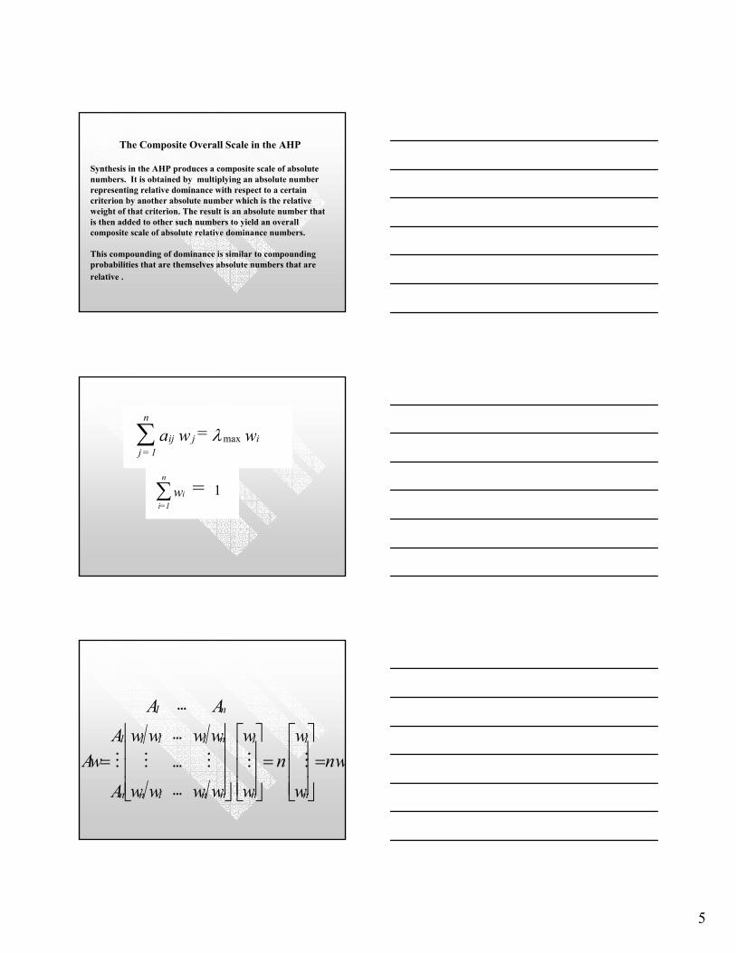
The Composite Overall Scale in the AHP
Synthesis in the AHP produces a composite scale of absolutenumbers. It is obtained by multiplying an absolute number representing relative dominance with respect to a certaincriterion by another absolute number which is the relativeweight of that criterion. The result is an absolute number thatis then added to other such numbers to yield an overall composite scale of absolute relative dominance numbers.
This compounding of dominance is similar to compounding probabilities that are themselves absolute numbers that arerelative .
w = w a ijij
n
1 =j λmax∑
1 = wi
n
1=i∑
... ...... ...
1 n
1 1 1 1 n 1 1
n n 1 n n n n
A Aw w w w w wA
Aw n nww w w w w wA
= = =
M M M M M
6
12 1
12 2
1 2
1 ...1/ 1 ...
1/ 1/ ... 1
n
n
n n
a aa a
A
a a
=
M M M M
ija jiai
Let A1, A2,…, An, be a set of stimuli. The quantified judgments on pairs of stimuli Ai, Aj, are represented by an n-by-n matrix A = (aij), ij = 1, 2, . . ., n. The entries aij are defined by the following entry rules. If aij = a, then aji = 1 /a, a 0. If Ai is judged to be of equal relative intensity to Aj then aij = 1, aji = 1, in particular, aii= 1 for all i.
Clearly in the first formula n is a simple eigenvalue and all other eigenvalues are equal to zero.
A forcing perurbation of eigenvalues theorem:
If λ is a simple eigenvalue of A, then for small ε > 0, there is an eigenvalue λ(ε) of A(ε) with power series expansion in ε:
λ(ε)= λ+ ε λ(1)+ ε2 λ(2)+…
and corresponding right and left eigenvectors w (ε) and v (ε) such that w(ε)= w+ ε w(1)+ ε2 w(2)+…
v(ε)= v+ ε v(1)+ ε2 v(2)+…
Aw=nw
Aw=cw
Aw=λmaxw
How to go from
to
and then to
max .1
nn
λµ
−≡
−
On the Measurement of Inconsistency
A positive reciprocal matrix A has with equality if and only if A is consistent. As our measure of deviation of A from consistency, we choose the consistency index
max nλ ≥
7
so and is the average of
the non- principal eigenvalues of A.
∑=
+=n
iin
2max λλ
2
11
n
iin
µ λ=
− = ∑−∑
=
=−n
iin
2max λλ
We know that and is zero if and only if A is consistent. Thus the numerator indicates departure from consistency. The term “n-1” in the denominator arises as follows: Since trace (A) = n is the sum of all the eigenvalues of A, if we denote the eigenvalues of A that are different from λmax by λ2,…,λn-1, we see that ,
0≥µ
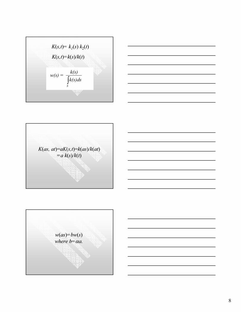
w(s) = dt w(t)t)K(s, b
a
λmax∫
w(s)= t)w(t)dtK(s, b
a∫λ
1 = w(s)dsb
a∫
The Continuous Case
KK((s,ts,t)) KK((t,st,s)) = = 1 1
KK((s,ts,t)) KK((t,ut,u))= K= K((s,us,u), ), for all for all s, t,s, t, and and uu
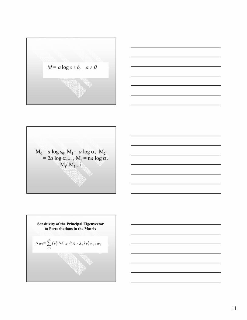
The periodic function is bounded and the negative exponential gives rise to an alternating series. Thus, to a first order approximation this leads to the Weber-Fechner law:
bsa +log
r)+(1s= sss+ s= s+ s= s0
0000011
∆∆
The Weber-Fechner law: Deriving the Scale 1-9
10
α 20
201112 s)r+(1s = r)+(1s = s+s = s ≡∆
2,...) 1, 0, = (n s = s = s n01-nn αα
α s -s = n 0n
log)log(log
11
0a b,+ s a = M ≠log
MM0 0 = = aa log slog s00, M, M1 1 = = aa log log αα, M, M22= 2= 2aa log log αα,... , ,... , MMnn = = nnaa log log αα..
Mi/ M1 = i
w)wv )-/(w A v( = w jjTjj11
Tj
n
2j=1 λλ∆∆ ∑
Sensitivity of the Principal Eigenvector to Perturbations in the Matrix
12
.WB...BB = W ,1+p1-qq
.WB...BB = W ,21-hh
Choosing the Best House
Price RemodelingCosts
Size(sq. ft.)
Style
200300500
15050
100
300020005500
ColonialRanch
Split Level
ABC
Figure 1.Figure 1. Ranking Houses on Four CriteriaRanking Houses on Four CriteriaWe must first combine the economic factors so we have threecriteria measured on three different scales. Two of them are tangible and one is an intangible. The tangibles must be measuredin relative terms so they can be combined with the priorities ofthe intangible.
In relative terms, the normalized sums should be
350/1300 .269350/1300 .269600/1300 .462
200 + 150 = 350300 + 50 = 350500 + 100 = 600
Combining the two economic criteria into a single criterion
13
Choosing the Best House
Price Remodeling Size(sq. ft.)
Style
200/1000300/1000500/1000
150/30050/300100/300
300020005500
ColonialRanch
Split Level
ABC
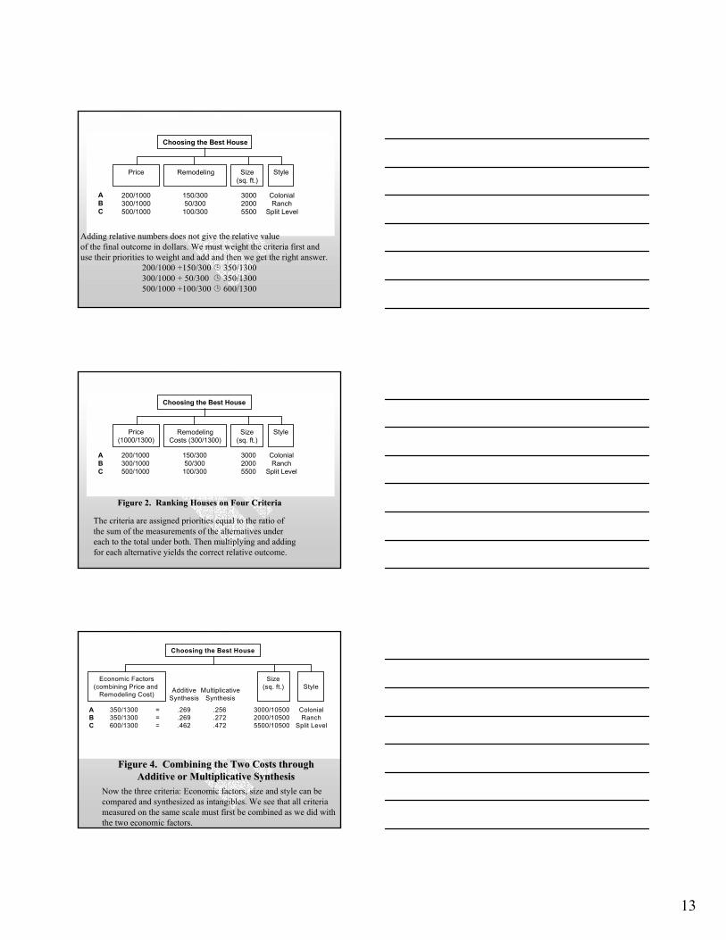
Adding relative numbers does not give the relative value of the final outcome in dollars. We must weight the criteria first and use their priorities to weight and add and then we get the right answer.
Figure 2.Figure 2. Ranking Houses on Four CriteriaRanking Houses on Four Criteria
The criteria are assigned priorities equal to the ratio ofthe sum of the measurements of the alternatives under each to the total under both. Then multiplying and addingfor each alternative yields the correct relative outcome.
Figure 4. Combining the Two Costs through Figure 4. Combining the Two Costs through Additive or Multiplicative SynthesisAdditive or Multiplicative Synthesis
Choosing the Best House
Economic Factors(combining Price and
Remodeling Cost)
Size(sq. ft.) Style
350/1300350/1300600/1300
.269
.269
.462
3000/105002000/105005500/10500
ColonialRanch
Split Level
ABC
===
AdditiveSynthesis
MultiplicativeSynthesis
.256
.272
.472
Now the three criteria: Economic factors, size and style can be compared and synthesized as intangibles. We see that all criteriameasured on the same scale must first be combined as we did withthe two economic factors.
14
x a=)a-x a( +1 x a +1 )x a( =)x ( = x = x
iiiii
iiiiia
ia
ia iii
∑∑≈∑≈∑∑∏∏ loglogexplogexplogexp
x x x = ) x , ,x ,x( f qn
q2
q1n21
n21 KK
γ γγγ x q + x q + x q = ) x , ,x ,x( f nn2211n21 KK
where qwhere q11+q+q22+...++...+qqnn=1, =1, qqkk>0 (k=1,2,...,n), >0 (k=1,2,...,n), γγ > 0, but > 0, but otherwise qotherwise q11,q,q22,...,,...,qqnn,,γγ are arbitrary constantsare arbitrary constants
15
11
=∑=
m
iia
x ..., ,x (i)n
(i)1
Π
Π x
1=i
m ..., ,x
1=i
man
a1
ii
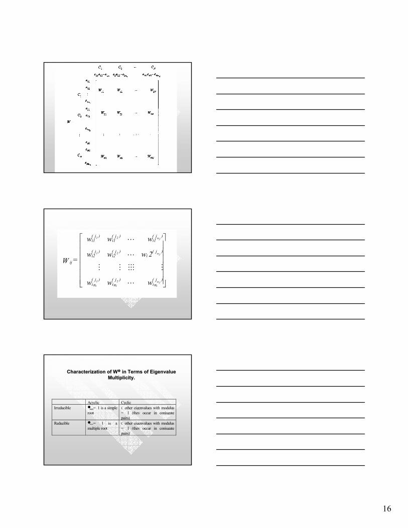
16
www
2www
www
= W
)j(ni
)j(ni
)j(ni
)j(i
)j(i2
)j(i2
)j(i1
)j(i1
)j(i1
ij
n ji
2i
1i
n j21
n j21
K
MMMMMM
K
K
Acyclic CyclicIrreducible max= 1 is a simple
rootC other eigenvalues with modulus= 1 (they occur in conjugatepairs)
Reducible max= 1 is amultiple root
C other eigenvalues with modulus= 1 (they occur in conjugatepairs)
Characterization of WCharacterization of W in Terms of in Terms of EigenvalueEigenvalueMultiplicity.Multiplicity.